INTRODUCTION
The risk assessment of a genetically modified (GM) crop and the derived products for food and animal feed begins with hazard identification, which is facilitated by evaluating the safety of samples collected from a multi-site field study (König et al. Reference König, Cockburn, Crevel, Debruyne, Grafstroem, Hammerling, Kimber, Knudsen, Kuiper, Peijnenburg, Penninks, Poulsen, Schauzu and Wal2004; EFSA 2010). The concept of substantial equivalence is the principal guidance for this safety evaluation (OECD 1993; Codex Alimentarius Commission 2009). It assesses safety with respect to key agronomic, phenotypic and compositional characteristics specific to the crop species. For a given endpoint, equivalence is established if the genetically modified organism (GMO) gives values similar to the non-GM isogenic/near-isogenic comparator or within the natural variation of non-GM reference crops with a history of safe use. Endpoints with uncertain equivalence are subjected to hazard characterization that involves animal testing of the whole food (EFSA 2008, 2014) and exposure assessment.
The multi-site study of crop safety typically plants GMO, the non-GM counterpart and several references together at each site according to a randomized block design. Suppose M endpoints are analysed by the linear mixed model. Let
 $\mu _{\rm T}^m $
and
 $\mu _{\rm C}^m $
be the mean of GMO (the test product) and the non-GM counterpart (the control) for endpoint m, m = 1, …, M. Traditionally, substantial equivalence has been established via a procedure that entails testing statistically whether
 $\mu _{\rm T}^m $
is identical to
 $\mu _{\rm C}^m $
. The following hypotheses describe the null (denoted by H) and alternative (denoted by K) of this difference test.
 $$H_{{\rm TC}}^m :\mu _{\rm T}^m - \mu _{\rm C}^m = 0\;v.\;K_{{\rm TC}}^m :\mu _{\rm T}^m - \mu _{\rm C}^m \ne 0$$
Retaining
 $H_{{\rm TC}}^m $
is taken as no difference and therefore equivalent. Only endpoints with rejected
 $H_{{\rm TC}}^m $
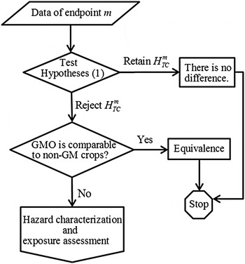
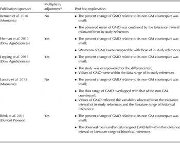
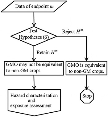
are evaluated further, in a post hoc manner, under the context of biological relevance and natural variation of non-GM crops. Table 1 cites several sponsors’ strategies for exempting endpoints from hazard characterization and exposure assessment. Note that some sponsors adjusted P values for testing hypotheses (1) by controlling the false discovery rate (FDR) (Benjamini & Hochberg Reference Benjamini and Hochberg1995). As indicated by the flow chart of this process (Fig. 1), conclusions of safety were based on either non-significant results or various subjective explanations.
Flow chart for the traditional process that focuses on the difference test. This process compares genetically modified organisms (GMO) to non-GM crops in a post hoc manner using various subjective explanations.

Traditional strategies to exclude GMO endpoints from hazard characterization and exposure assessment

GMO, genetically modified organism.
* Multiplicity adjustment controls the false discovery rate in testing hypotheses (1) across endpoints.
The European Food and Safety Authority (EFSA) mandates a procedure that entails two types of comparisons (EFSA 2010). The first type compares GMO with the non-GM counterpart. It is formulated as hypotheses (1) except that parameters here pertain to the mixed model for natural-log-transformed data. The EFSA recommends a log transformation for data measured on a continuous scale because (1) many biological effects are multiplicative rather than additive; (2) transformed data tends to become homoscedastic; (3) normality seems to be better achieved upon transforming the compositional data. Statistical testing is set at the 0·10 significance level for each endpoint. The EFSA considers FDR adjustment to difference tests insufficient for GMO risk assessment. Instead, re-sampling is used to determine how likely it is to attain the observed number of endpoints with a significant difference under the assumption that
 $\mu _{\rm T}^m - \mu _{\rm C}^m $
has a zero-mean normal distribution. The second type compares GMO with references grown concurrently in the study. Let
 $\mu _{\rm R}^m $
be the reference mean. The guidance tests equivalence, i.e.
 $$H_{{\rm TR}}^m :\left \vert {\mu _{\rm T}^m - \mu _{\rm R}^m} \right \vert \ge \hat EL\;v.\;K_{{\rm TR}}^m :\left \vert {\mu _{\rm T}^m - \mu _{\rm R}^m} \right \vert \lt \hat EL$$
and non-equivalence, i.e.
 $$H_{{\rm TR}}^m :\left \vert {\mu _{\rm T}^m - \mu _{\rm R}^m} \right \vert \le \hat EL\;v.\;K_{{\rm TR}}^m :\left \vert {\mu _{\rm T}^m - \mu _{\rm R}^m} \right \vert \gt \hat EL$$
where
 $\hat EL$
is the equivalence limit (EL) estimated from the observed natural variation of in-study references. The guidance suggests applying FDR-controlling procedures to adjust equivalence tests across endpoints, but leaves this option open for future improvement. By the two one-sided tests (TOST) of Schuirmann (Reference Schuirmann1987), the null in hypotheses (2) or (3) is rejected at the 0·05 significance level if the 90% confidence interval (CI) of
 $\mu _{\rm T}^m - \mu _{\rm R}^m $
is totally within or outside
 $( - \hat EL,\hat EL)$
. If both nulls are retained, comparison of the point estimate of
 $\mu _{\rm T}^m - \mu _{\rm R}^m $
with
 $( - \hat EL,\hat EL)$
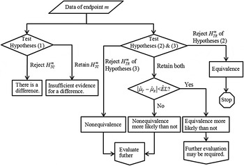
leads to the conclusion of ‘equivalence more likely than not’ or ‘non-equivalence more likely than not’. The flow chart of this process (Fig. 2) indicates a series of issues in EFSA's comparative analysis. Ignoring the uncertainty in estimating
 $\hat EL$
makes the actual type I error rate intractable (Kang & Vahl Reference Kang and Vahl2014). Testing for non-equivalence contributes little in deciding whether to evaluate further, since EFSA requests more investigation as either a must or a maybe for endpoints lacking the conclusion of equivalence. The assertion of ‘more likely than not’, when both nulls are retained, makes sense only when one considers parameters to be random quantities with a posterior probability distribution. It is a Bayesian interpretation and does not belong to the realm of frequentist inference. Moreover, using both 0·10 and 0·05 significance levels in the same study is unconventional and difficult to defend. For endpoints with retained nulls of hypotheses (2) and (3), EFSA encourages sponsors to incorporate results of the two types of comparisons when deciding whether to proceed with hazard characterization and exposure assessment. Yet there has been no detailed instruction on how to interpret these results. In July 2015, nine non-government organizations requested the European Commission to review the authorization for the import of a GM oilseed rape. Uncertainty in the statistical analysis was one of the filed complaints (EFSA 2015a
).
Flow chart for the process mandated by EFSA (2010). Label ‘^˄’ distinguishes estimated parameters from their true values.

The safety evaluation of a GM crop is inherently a decision-making process with a confirmatory nature. Multiple testing procedures (MTPs) strive to assure that results concluded from a single study are replicable. Often this is achieved by strongly controlling the familywise error rate (FWER), i.e. limiting the maximum probability of making at least one wrong inference under any configuration of nulls. Properly stating hypotheses according to the study objective constitutes an intrinsic, crucial element in creating MTPs. When hypotheses (1) are used to establish substantial equivalence, the corresponding multiplicity adjustment controls the probability of wrongfully concluding that the genetic engineering has changed the crop in at least one endpoint. This error rate corresponds to the sponsor's risk. However, the more important error to control is the consumer's risk, i.e. the probability of erroneously asserting equivalence on one or more potentially hazardous endpoints. Adjusting for multiplicity in testing hypotheses (1) is a mismatch for the study objectives. Although a strong FWER control is indispensable for studies at the confirmatory stage, many practitioners consider it counterproductive in exploratory research. The FDR, on the other hand, is an alternative error rate definition that has gained popularity in analysing high-dimensional data generated by high-throughput technologies. It refers to the expected proportion of false rejections among all rejected nulls. Adjustment of FDR has attracted attention from both the ag-biotech industry and EFSA, albeit for controlling different types of risk. Note that FDR-controlling MTPs attain better power at the expense of the FWER. Finner & Roters (Reference Finner and Roters2001) further reveal that the FDR is susceptible to ‘cheating’ by adding irrelevant hypotheses with almost sure rejection. Hence, regulatory guidance on confirmatory clinical trials requests control of the FWER (CPMP 2002; FDA 2009; also see Hsu Reference Hsu2010 for a succinct introduction on this topic). Provided hypotheses for crop safety evaluation are well formulated, a strong control on the FWER is capable of restricting the consumer's risk in the worst-case scenario and better addresses the public's rising concerns on food safety. Hence, FDR-controlling procedures ought to be avoided in establishing substantial equivalence.
Two sources of multiplicity exist in GMO testing from field trials. One obvious source comes from the many endpoints under evaluation. The other, which has not received much attention, arises from the comparisons of GMO v. the non-GM counterpart and again v. the references. Previous evaluations have mishandled the latter source with a barrage of post hoc explanations. There is certainly ample opportunity to strengthen the scientific integrity of this process. Simple, off-the-shelf MTPs are, nonetheless, inadequate to handle this complex multiplicity problem. A general strategy for creating MTPs has been outlined in the context of clinical trials (Chi Reference Chi1998; Dmitrienko et al. Reference Dmitrienko, Offen and Westfall2003; Chen et al. Reference Chen, Capizzi, Binkowitz, Quan, Wei and Luo2005; Hung & Wang Reference Hung and Wang2009, Reference Hung and Wang2010). There, the sponsor converts the overall objective of the study into a list of explicit claims and organizes them as a set of decision rules. The statistician translates these claims and decision rules into hypotheses interlinked by logical operators. An MTP is then created to suit the specific layout of these hypotheses. Given the observed data, the decision-making process is solely driven by the multiplicity-adjusted statistical results. Specification of the MTP upfront without any post hoc alterations is thus critically important for preserving the FWER. Strategic planning of the MTP not only motivates a process with logical flow but also reduces conservativeness in multiplicity adjustment. Many customized MTPs have been created for various clinical studies with several sources of multiplicity (a comprehensive review is available in Dmitrienko et al. Reference Dmitrienko, D'Agostino and Huque2013). These studies all entail efficacy assessment whose objectives and decision rules differ fundamentally from safety evaluation. Statistical methods have also been developed for exploratory analyses of drug adverse events obtained from clinical efficacy trials and post-marketing spontaneous reports (Berry & Berry Reference Berry and Berry2004; Mehrotra & Heyse Reference Mehrotra and Heyse2004; Gould Reference Gould2008; Huang et al. Reference Huang, Zalkikar and Tiwari2011). These types of safety assessment avoid formal hypothesis testing and FWER control. A new MTP is needed particularly for establishing GMO substantial equivalence based on endpoints measured from crop field trials.
The current paper aims to develop statistical strategies for adjusting multiplicity in the safety evaluation of a GM crop. For each comparison at every endpoint, individual hypotheses are explicitly defined to mirror the study objectives. Guided by the decision rules currently in use, these hypotheses are grouped into families and linked by logical operators to form composite hypotheses. This objective testing of pre-specified hypotheses arranged in an organized layout results in a transparent evaluation process where the consumer's risk can be directly controlled. A two-stage MTP tailored specifically to the unique hypothesis layout is then created by applying fundamental principles for multiple testing. The newly proposed MTP is simple to implement and communicate. Its utility is shown in a real-world example, dismissing the concern that a statistical conclusion of safety is hopelessly unattainable via multiple equivalence testing. Finally, the proposed MTP is discussed in regard to its potential improvements and additional generalizations.
MATERIALS AND METHODS
Formulating individual hypotheses
The logic of hypothesis testing places the target assertion into the alternative hypothesis. Everything else within the parameter space of interest goes into the null. The sponsor of an efficacy study supports its product's regulatory approval by rejecting the null of zero-difference. The sponsor of a safety study should firmly defend its product's authorization by rejecting the null of non-equivalence, rather than blindly adopting the hypotheses in the efficacy study and wishing for non-significance. Defining safety in terms of equivalence is not without precedence. For example, Hsu & Berger (Reference Hsu and Berger1999) advocate tests of practical equivalence in assessing the toxicity of bovine growth hormone. Oberdoerfer et al. (Reference Oberdoerfer, Shillito, Beuckeleer and Mitten2005) were the first to apply equivalence testing to crop safety evaluation. Practitioners, on the other hand, are often attracted by the mathematical convenience in testing for difference and avoid equivalence testing due to complications in defining appropriate ELs. Blunt advice against reliance on such ill-posed hypotheses is to cite Hsu (Reference Hsu1996): ‘an approximate solution to the right problem … will be better than an exact solution to the wrong problem, the latter accounting for a significant portion of the abuse.’
Table 1 shows a consensus that
 $\mu _{\rm T}^m - \mu _{\rm C}^m $
must be small to establish equivalence. The present work proposes to compare GMO with the non-GM counterpart at endpoint m by testing
 $$H_{{\rm TC}}^m :\left \vert {\mu _{\rm T}^m - \mu _{\rm C}^m} \right \vert \ge \delta _0\;v.\;K_{{\rm TC}}^m :\left \vert {\mu _{\rm T}^m - \mu _{\rm C}^m} \right \vert \lt \delta _0$$
Value δ
0 defines a ‘zone of indifference’ where differences inside it are considered trivial for practical purposes. It establishes similarity, or practical equivalence, but has no direct implications on safety. Because
 $\mu _{\rm T}^m $
and
 $\mu _{\rm C}^m $
are parameters in the mixed model analysis of the log-transformed data, [exp (δ
0) − 1] represents the largest tolerated change of GMO relative to the non-GM counterpart in terms of their back-transformed, i.e. geometric, means. The EFSA guidance used ‘percent change (e.g. −20% and +25%) for relatively small changes, or factors (e.g. ½ and 2) for larger changes’ whereas Oberdoerfer et al. (Reference Oberdoerfer, Shillito, Beuckeleer and Mitten2005) used ±20%. A working δ
0 could then be set as ln(1.25) or ln(1.20). Hypotheses (4) cannot be used as the sole component for establishing equivalence at a given endpoint, because it does not incorporate crop's natural variation. Hothorn & Oberdoerfer (Reference Hothorn and Oberdoerfer2006) explored several options for defining endpoint-specific ELs. Unfortunately, these definitions fall short in biological validity or statistical rigour.
The current paper addresses natural variation through additional hypotheses that compare GMO with references. As mentioned earlier, crop safety studies employ the multi-site design where various references and GMO are randomized into plots arranged in blocks at each site. Under the linear mixed model of EFSA, natural variation can be easily incorporated into the EL. Vahl & Kang (Reference Vahl and Kang2016) introduced the following hypotheses to assess the equivalence of GMO to references at endpoint m.
 $$\hskip--8.15ptH_{{\rm TR}}^m :\left \vert {\mu _{\rm T}^m - \mu _{\rm R}^m} \right \vert \ge \sqrt {\Delta (\vartheta, {\bf \sigma}^m )} \;v.\quad\;K_{{\rm TR}}^m :\left \vert {\mu _{\rm T}^m - \mu _{\rm R}^m} \right \vert \lt \sqrt {\Delta (\vartheta, {\bf \sigma}^m )} $$
Function Δ( · ) corresponds to the EL for
 $(\mu _{\rm T}^m - \mu _{\rm R}^m )^2$
. Its argument
 $\vartheta $
is a value to be specified by the regulatory agency. Vector
 ${\bf \sigma}^m = (\sigma _S^m, \sigma _{{\rm B}(S)}^m, \sigma _{\rm R}^m, \sigma _{\rm E}^m )$
denotes the parameter of natural variation due to site, block-within-site, reference genotype and experimental error terms. Van der Voet et al. (Reference Van der Voet, Perry, Amzal and Paoletti2011) consider ‘appropriate percentiles (e.g. 2·5 and 97·5) of the distribution of reference variety characteristics’ as the limits of
 $\mu _{\rm T}^m $
. Denote z
0.975 as the 97·5th percentile of the standard normal distribution. Setting
 $\Delta (z_{0.975},{\bf \sigma} ^m) = z_{0.975}^2 [(\sigma _{\rm R}^m )^2 + (\sigma _{\rm E}^m )^2]$
restricts
 $\mu _{\rm T}^m $
to be within the 2·5th and 97·5th percentiles of the reference distribution at the site and block level. Vahl & Kang (Reference Vahl and Kang2016) referred to this as conditional scaled average equivalence. Percentiles of the marginal distribution of references are more pertinent to safety. This choice leads to the notion of marginal scaled average equivalence with
 $\Delta (z_{0.975},{\bf \sigma} ^m) = z_{0.975}^2[(\sigma _{\rm S}^m )^2 + (\sigma _{{\rm B}({\rm S})}^m )^2 + (\sigma _{\rm R}^m )^2 + (\sigma _{\rm E}^m )^2]$
. Nevertheless, current field designs impede the proper quantification of
 $\sigma _{\rm S}^m $
. Because conditional equivalence implies marginal equivalence, a more practical and conservative EL for hypotheses (5) is
 $\Delta (z_{0.975},{\bf \sigma} ^m) = z_{0.975}^2 [(\sigma _{\rm R}^m )^2 + (\sigma _{\rm E}^m )^2]$
.
The EFSA guidance also tests non-equivalence, whose hypotheses reverse the null and alternative of the equivalence test. While an improvement over a simple test of zero-difference, this test of non-equivalence is still a mismatch with the proof-of-safety objective. It represents the subconscious reversion to traditional exploratory toxicity studies with a proof-of-hazard purpose (Hothorn & Hasler Reference Hothorn and Hasler2008). Note that
 $\Delta (\delta, {\bf \sigma} ^m)$
is not an exact rigid threshold for toxicity but rather a conservative soft limit of safety. Non-significant evidence for equivalence logically suggests further evaluation, whereas a conclusion of non-equivalence invites misinterpretation as established true hazard. Moreover, simultaneously testing two opposing objectives (hazard and safety) complicates the statistical decision-making process and hinders straightforward characterization of the consumer's risk. For these reasons, non-equivalence tests should be omitted in crop safety evaluation.
In a three-arm non-inferiority study of drug efficacy, non-inferiority of the test treatment to the active control relies on the assay sensitivity, which can be validated by testing the superiority of the active control over the placebo (Röhmel & Pigeot Reference Röhmel and Pigeot2010 and the literature cited therein). This is founded on the concern that the active control may not be efficacious in the current study. A similar question is whether to compare GMO with references if the non-GM counterpart is not significantly equivalent to references under the same criterion. Unlike the active control and placebo in drug efficacy studies, both the non-GM counterpart and references are safe, a priori. It is unnecessary to test the non-GM counterpart against references and this question is moot.
Grouping hypotheses into families
Tamhane (Reference Tamhane, Ghosh and Rao1996) defines a family as a set of comparisons from which some common conclusions are drawn and states that comparisons within this family must be contextually related but not necessarily statistically dependent. Grouping of individual hypotheses into relevant families should match the study objective and decision rule. Recall that M endpoints are subjected to mixed model analyses. There are 2M individual hypotheses and as many as 22M
− 2M − 1 combinations to form composite hypotheses. One possible approach is to place comparisons involving the non-GM counterpart into one family, i.e.
 $\{ H_{{\rm TC}}^1 \;v.\;K_{{\rm TC}}^1,..., H_{{\rm TC}}^M \;vs.\;K_{{\rm TC}}^M \} $
, and comparisons involving references into another family, i.e.
 $\{ H_{{\rm TR}}^1 \;v.\;K_{{\rm TR}}^1,..., H_{{\rm TR}}^M \;v.\;K_{{\rm TR}}^M \} $
. The two families each contain M individual hypotheses. The EFSA guidance seems to adopt this approach. Nonetheless, the traditional industry practice and recent regulatory opinions indicate that the safety of a GM crop is evaluated at each specific endpoint (literature listed in Table 1; EFSA 2015a
,
b
,
c
, 2016). This supports grouping the two comparisons at a given endpoint into a family, i.e.
 $\{ H_{{\rm TC}}^m \;v.\;K_{{\rm TC}}^m, \;H_{{\rm TR}}^m \;v.\;K_{{\rm TR}}^m \} $
. Consequently, there are M families of hypotheses, each corresponding to an endpoint.
Members of a family can be linked by either intersection or union, which gives rise to two basic types of composite hypotheses: intersection-union (IU) and union-intersection (UI). The IU hypotheses place the intersection of individual alternatives in its alternative and the union of individual nulls in its null. It corresponds to an ‘each-and-every’ type of conclusion. In contrast, the UI hypotheses contain the union of individual alternatives in its alternative and the intersection of individual nulls in its null. It corresponds to an ‘at-least-one’ type of conclusion. Recall that GMO is regarded as safe if it is comparable with either the non-GM counterpart or references. Equivalence at a given endpoint shall then be formulated as the following local UI hypotheses.
 $$H^m :H_{{\rm TC}}^m \cap H_{{\rm TR}}^m \;v.\;K^m :K_{{\rm TC}}^m \cup K_{{\rm TR}}^m $$
To those who presume hypotheses (5) as a relaxation of hypotheses (4) (i.e.
 $K_{{\rm TC}}^m \subset K_{{\rm TR}}^m $
), hypotheses (6) seem unnecessary since
 $K_{{\rm TC}}^m \cup K_{{\rm TR}}^m = K_{{\rm TR}}^m $
. However, experience with GMO safety analyses suggests that
 $K_{{\rm TC}}^m \cup K_{{\rm TR}}^m \supset K_{{\rm TR}}^m $
. Insight on this is gained by depicting hypotheses (4–6) at endpoint m as partitions in a two-dimensional space. Given the known safety of the non-GM counterpart,
 $\mu _{\rm C}^m $
is expected to be not far from
 $\mu _{\rm R}^m $
. It is then convenient to express
 $\mu _{\rm T}^m - \mu _{\rm C}^m $
as
 $(\mu _{\rm T}^m - \mu _{\rm R}^m ) - (\mu _{\rm C}^m - \mu _{\rm R}^m )$
and examine the parameter space of
 $(\mu _{\rm T}^m - \mu _{\rm R}^m, \;\mu _{\rm C}^m - \mu _{\rm R}^m )$
. In this way, the entire parameter space of interest,
 $H^m \cup K^m $
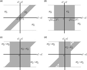
, is simply represented by the horizontal strip in between the two dashed lines in Fig. 3. Boundaries of
 $H^m \cup K^m $
reflect the fact that the non-GM counterpart is as safe as any non-GM reference variety. They represent the unknown safety limits, which are less stringent than the ELs in hypotheses (5). The
 $K_{{\rm TC}}^m $
space is represented by the shaded thin parallelogram in Fig. 3(a) and the
 $K_{{\rm TR}}^m $
space is given by the shaded tall rectangle in Fig. 3(b). Visibly, the
 $K_{{\rm TC}}^m $
space is not nested within
 $K_{{\rm TR}}^m $
. Depending on the width of the
 $K_{{\rm TR}}^m $
rectangle, the
 $K^m $
space takes two shapes (Figs 3(c) and (d)). The set difference between
 $K_{{\rm TC}}^m \cup K_{{\rm TR}}^m $
and
 $K_{{\rm TR}}^m $
, i.e.
 $(K_{{\rm TC}}^m \cup K_{{\rm TR}}^m )\backslash K_{{\rm TR}}^m $
, is non-empty and serves as a compensation when
 $\mu _{\rm C}^m $
is not very close to
 $\mu _{\rm R}^m $
. Particularly, Fig. 3(d) displays the situation of an overly conservative EL. In such a case, hypotheses (5) alone do not adequately represent the concept of substantial equivalence. Testing hypotheses (6) yields a reasonable solution. Tolerance intervals or literature ranges derived from non-GM crops are random quantities with intractable uncertainty. Because their usage is less transparent and prone to manipulation, the present work excludes them from the decision-making process. Figure 4 presents the flow chart for the proposed evaluation. Here the two partial decisions at endpoint m are integrated into a joint decision of overall equivalence by testing the local UI hypotheses. This supports a decision-making process on the basis of pre-specified justification rather than post hoc arguments. It is clearly an improvement over those processes in Figs 1 and 2.
Graphic representation of (a) hypotheses (4), (b) hypotheses (5), (c) hypotheses (6) with
 $\Delta (z_{0.975},{\bf \sigma} ^m)$
representative of the natural variation and (d) hypotheses (6) with a conservative
 $\Delta (z_{0.975},{\bf \sigma} ^m)$
. Area between the dashed lines is the parameter space of interest. Shaded area represents the alternative space of the corresponding hypotheses.

Flow chart for the process that jointly compares genetically modified organisms (GMO) with the non-GM counterpart and references.

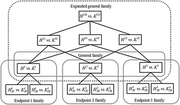
Testing hypotheses (6) across M endpoints pertains to a new family of hypotheses. Figure 5 visualizes the organized layout at M = 3. Here the individual hypotheses are grouped into endpoint-specific families of hypotheses, whose UI composites then form a general family. Now the question is how to link members in this general family. Because equivalence at every endpoint implies global equivalence, one might consider the following global IU hypotheses.
 $$H:\bigcup\nolimits_{m = 1}^M {H^m} \;v.\;K:\bigcap\nolimits_{m = 1}^M {K^m} $$
The organized layout representing the families of hypotheses in establishing substantial equivalence with respect to three endpoints.

Rejecting the null of hypotheses (7) would be a big win for the sponsor. But failing to do so does not result in an automatic regulatory denial, as hazard characterization and exposure assessment will be undertaken for endpoints that cause the null to be retained. Hypotheses (7) do not allow for endpoint-specific conclusions and are therefore a mismatch for crop safety evaluation. Moreover, the type I error in testing hypotheses (7) refers to the assertion of global equivalence when non-equivalence occurs in some endpoints. Its probability does not correspond to the consumer's risk in hazard identification, i.e. the probability of erroneously asserting equivalence on one or more non-equivalent endpoints. According to the theoretical findings of Sonnemann & Finner (Reference Sonnemann, Finner, Bauer, Hommel and Sonnemann1988), strong control on the error of rejecting at least one true H m can be achieved by adding the following UI composite hypotheses to the general family (see Fig. 5) and testing each H m via the well-established closure principle (a brief introduction on this principle is available in Appendix 1).
 $$H^I:\bigcap\nolimits_{m \in I}^{} {H^m} \;v.\;K^I:\bigcup\nolimits_{m \in I}^{} {K^m} $$
The index set I here is a subset of {1, …, M}. For M = 3, I = {1, 2}, {1, 3}, {2, 3}, {1, 2, 3}. Linking K
m
by ‘
 $ \cup $
’ may be difficult for some to comprehend, as these hypotheses are themselves of little practical interest. Nonetheless, expanding the general family to include UI hypotheses allows strong FWER control without compromising the power. In other words, testing such an expanded family of hypotheses is as good as testing the family with individual hypotheses only. It is worthwhile to mention that similar UI formulation of composite hypotheses is becoming increasingly common in multi-endpoint bioequivalence and non-inferiority studies of drugs (Quan et al.
Reference Quan, Bolognese and Yuan2001; Logan & Tamhane Reference Logan and Tamhane2008; Hasler & Hothorn Reference Hasler and Hothorn2013; Hua et al.
Reference Hua, Xu and D'Agostino2015). This stems from the need for inference on individual endpoints.
The multiple endpoints in drug safety evaluation, i.e. types of adverse events, can be categorized into several body systems on the basis of prior clinical understanding. Such grouping has been used to reduce false positive findings (Berry & Berry Reference Berry and Berry2004; Mehrotra & Heyse Reference Mehrotra and Heyse2004). However, the intertwining relationship of plant metabolic pathways prevents any grouping of endpoints measured in crop safety evaluation. Consequently, there is no intermediate grouping of hypotheses (6) into subfamilies. Only the family containing hypotheses (6) across all endpoints is relevant for GMO testing.
A multiple testing procedure for genetically modified organism safety evaluation
There are three fundamental principles governing multiple testing in the UI context. The closure principle establishes the general method for MTP construction. The sequential rejection principle and the partition principle exploit the relationships among individual hypotheses to improve power. A brief tutorial of these principles and their applications is given in Appendix 1. As mentioned previously, hypotheses (4) and (5) at a given endpoint are not nested. Neither sponsors nor regulatory agencies have articulated any decision path among endpoints measured in crop safety evaluation. This prevents hypotheses (6) from being arranged, in advance, into a fixed sequence. Sequential testing in a data-driven order is therefore the best available approach here. Practitioners accustomed to the analysis of variance setting may be familiar with Dunnett's parametric stepwise procedures used in comparing several treatments with a control (Dunnett & Tamhane Reference Dunnett and Tamhane1991, Reference Dunnett and Tamhane1992). Construction of these MTPs relies on the knowledge that the individual test statistics have a joint multivariate t distribution. The distinct formulation of hypotheses (4) and (5) makes it difficult to characterize such a joint distribution. The Simes-Hochberg (SH) procedure is a classical semi-parametric sequential MTP (Westfall et al. Reference Westfall, Tobias, Rom, Wolfinger and Hochberg1999; Dmitrienko et al. Reference Dmitrienko, D'Agostino and Huque2013). It circumvents the derivation of any joint distribution and is readily applicable to GMO testing. Appendix 1 provides the generic formula for the SH adjustment. Multiplicity adjustment can be carried out by either raising the P values or dropping the significance levels of individual tests. Because these two approaches yield identical conclusions, only the P-value-based approach is presented.
To accommodate the hypothesis layout in Fig. 5, the present work proposes a two-stage MTP that executes the SH adjustment in both stages. The first stage derives the raw P value for testing hypotheses (6) at each endpoint. Suppose that the ordered P values for testing hypotheses (4) and (5) at endpoint m are
 $P_{(1)}^m $
and
 $P_{(2)}^m, P_{(1)}^m \le P_{(2)}^m $
. According to the SH adjustment, the raw P value for testing hypotheses (6) is:
 $$P^m = \min (2P_{(1)}^m, P_{(2)}^m )$$
Let
 $P^{(m)} $
be the m
th
smallest P value of
 $\{ P^1,..., P^M\} $
, i.e.
 $P^{(1)} \le \ldots \le P^{(M)}$
. The second stage controls the consumer's risk by correcting for multiplicity across endpoints. The SH method is applied for a second time and P values for hypotheses (6) are adjusted sequentially as:
 $$\eqalign{&\tilde{P}^{(m)} =\cr & \left\{\matrix{P^{(M)} &m = M \cr \min [\tilde{P}^{(m + 1)}, (M - m + 1)P^{(m)}] &1 \le m \le M - 1} \right.}$$
To preclude logical incoherence, this present work applies the closure principle and readjusts P values for individual hypotheses as:
 $$\eqalign{& \tilde P_{(1)}^{(m)} = \max (\tilde P^{(m)}, P_{(1)}^{(m)} ) \cr & \tilde P_{(2)}^{(m)} = \max (\tilde P^{(m)}, P_{(2)}^{(m)} )} $$
This assures that at a given endpoint, the P value for testing hypotheses (6) will be no greater than either of the two for testing hypotheses (4) and (5). Consequently, if the null of hypotheses (6) is retained, the corresponding nulls of hypotheses (4) and (5) are both retained.
The SH procedure has been demonstrated to strongly control the FWER for a general class of positively correlated multivariate distributions, many of which are encountered in multiple testing situations (Sarkar & Chang Reference Sarkar and Chang1997; Sarkar Reference Sarkar1998, Reference Sarkar, Balakrishnan, Peña and Silvapulle2008). Excessive ‘handwringing’ on its analytical conditions is counterproductive in practice. Biological rationale for the positive relationship among multiple inferences should alleviate any concern on its validity here. In particular, proper selection of GMO comparators, as articulated by EFSA (2011), assures
 $\mu _{\rm C}^m $
to be fairly close to
 $\mu _{\rm R}^m $
. Results of the two within-endpoint comparisons are therefore expected to be positively correlated. Owing to the intricacy of plant system biology, a positive relationship is also expected from results of equivalence testing across endpoints. It is therefore anticipated that the proposed MTP will restrain the FWER effectively. The large number of hypotheses tested (2M >100) obstructs non-parametric adjustments carried out either by the single-step Bonferroni (SSB) procedure or the sequential Bonferroni-Holm (BH) procedure. A similar viewpoint has been expressed by Hothorn & Oberdoerfer (Reference Hothorn and Oberdoerfer2006), who employed the SH procedure in their multiple testing of hypotheses (4) across compositional endpoints. For side-by-side comparisons of these procedures for a single family of hypotheses, see the corresponding formulas in Appendix 1. Let α be the desired FWER. The benefit of the proposed MTP is best seen when P
1, …,P
M
are all less than α. In this case, some of SSB- or BH-adjusted P values might be greater than α, which seems counterintuitive. The SH-adjusted P values, on the other hand, would always remain less than α. Such consistency among outcomes was recognized by Dmitrienko et al. (Reference Dmitrienko, D'Agostino and Huque2013) as a desirable property. It has served as an incentive for Quan et al. (Reference Quan, Bolognese and Yuan2001) and Hasler & Hothorn (Reference Hasler and Hothorn2013) to apply the SH adjustment in clinical equivalence and non-inferiority studies.
RESULTS
This section illustrates the newly developed MTP using a real-world dataset containing 53 compositional endpoints measured in a safety study on a GM maize. The EFSA guidance supplies the estimated
 $\mu _{\rm T}^m - \mu _{\rm C}^m $
and
 $\mu _{\rm T}^m - \mu _{\rm R}^m $
, their corresponding standard errors, the approximated degrees of freedom, and estimated variance components in the mixed model. These summary statistics are sufficient to test hypotheses (4) and (5). Suppose that GMO is comparable with the non-GM counterpart if the ratio of their geometric means is between 0·833 and 1·20. To account for natural variation, assume that 2·5th and 97·5th percentiles of the reference distribution at the site and block level are the ELs for the GMO geometric mean. These presumptions set δ
0 = ln(1.20) in hypotheses (4) and
 $\Delta (z_{0.975},{\bf \sigma} ^m) = z_{0.975}^2 [(\sigma _{\rm R}^m )^2 + (\sigma _{\rm E}^m )^2]$
in hypotheses (5). The P values associated with TOST for testing hypotheses (4) were computed via the method of Anderson & Hauck (Reference Anderson and Hauck1983). Appendix 2 exhibits their calculation using SAS (SAS Institute Inc 2011). The P values for testing hypotheses (5) were obtained by running the SAS program given in Kang & Vahl (Reference Kang and Vahl2016).
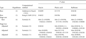
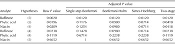
First, consider the simple case where crop safety was evaluated with respect to three analytes in the example dataset, namely, niacin, phytic acid and raffinose. Table 2 demonstrates how to manually implement the proposed two-stage MTP using the analytes’ raw P values for testing hypotheses (4) and (5). Note that stage two of this MTP utilized the ranking of analytes’ raw P values for testing Hypo (6) and made adjustments sequentially in the order of niacin, phytic acid and raffinose. Also note that the adjusted P value for testing hypotheses (5) of phytic acid (0·0418) was not a multiplier of its raw P value of 0·0196 but was borrowed from testing hypotheses (6) of niacin. Within each analyte, the adjusted P values for testing individual hypotheses maintained the same ranking as their corresponding raw P values; because these adjusted P values were never less than the P value for testing their composite UI hypotheses, retaining the null of hypotheses (6) coincided with retaining both nulls of hypotheses (4) and (5) at any given significance level. The proposed MTP thereby facilitates logical decision making. Table 3 compares this MTP to three basic MTPs applied naively without accounting for the decision rules in crop safety evaluation. It shows that basic MTPs preserved the ranking of the six raw P values but the two-stage MTP did not. In particular, there were three raw P values ranked in the order of 0·0238>0·0209>0·0196. The SSB procedure yielded adjusted P values in the same ranking, i.e. 0·1428>0·1254>0·1176. The BH and SH procedures adjusted them to a single value of 0·0980 and 0·0714, respectively. The two-stage MTP paired raw P values by analyte, i.e. 0·0238 with 0·0020, 0·0209 with 0·6652 and 0·0196 with 0·1119. Ultimately, 0·0238 was left as it is while 0·0209 and 0·0196 were raised to 0·0418. This new ranking is sensible, since 0·0020 is much smaller than 0·6652 and 0·1119. It is observed from Table 3 that in terms of the adjusted P values for an individual test, the four MTPs are ranked as SSB ⩾ BH ⩾ SH ⩾ two-stage. Bear in mind that the three basic MTPs control the error rate in testing six individual hypotheses whereas the two-stage MTP controls the error rate in testing three UI composites. The small adjusted P values of the two-stage MTP manifest the important strategy of dimension reduction suggested by Chi (Reference Chi1998). Organizing individual hypotheses according to decision rules, as in Fig. 5, reduces the composite hypotheses in a biologically relevant and meaningful way. The two-stage MTP provides the statistical support for this strategy.
Illustration of the two-stage multiple testing procedure for establishing crop substantial equivalence with respect to three analytes


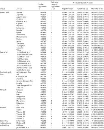
Next, evaluate crop safety with respect to all 53 analytes in the example dataset. Appendix 2 executes the proposed MTP using the SAS DATA step and MULTTEST procedure. Table 4 presents results of the two-stage multiple testing as well as the traditional difference test and the equivalence/non-equivalence tests of EFSA (2010). For reporting purposes, analytes were grouped by their chemical classification but the decision rules did not account for this grouping. Sixteen analytes had significant differences between
 $\mu _{\rm T}^m $
and
 $\mu _{\rm C}^m $
at the 0·05 significance level. Traditional evaluation concentrates on these analytes and will dismiss potential safety concerns with a bundle of non-statistical, post hoc explanations. The procedure mandated by EFSA tested hypotheses (2) and (3) by comparing the CIs of
 $\mu _{\rm T}^m - \mu _{\rm R}^m $
with estimated ELs. The P values of these tests were unavailable. Seven analytes were considered as ‘non-equivalence more likely than not’ or ‘equivalence more likely than not’. The guidance requested these analytes undergo further evaluation. Additionally, there were two analytes with zero estimated reference variability. They might also be subjected to further evaluation. However, a decision path for subsequent investigation remains elusive. The two-stage procedure led to a clear-cut conclusion: equivalence was significant at the 0·05 significance level in all 53 analytes. It was therefore unnecessary to conduct hazard characterization and exposure assessment. Tests for hypotheses (4) and (5) were both significant in 41 out of 53 analytes and 12 analytes had significance in only one of the two tests. For the 16 analytes where testing hypotheses (1) concluded significant difference, testing hypotheses (4) asserted practical equivalence between GMO and the non-GM counterpart in 13 analytes; testing hypotheses (5) declared GMO within the reference natural variation in 15 analytes. Regarding the 37 analytes with non-significant differences, three of them retained the null of hypotheses (4). It then comes as a reminder that non-significance in testing hypotheses (1) does not mean
 $\mu _{\rm T}^m $
is equivalent to
 $\mu _{\rm C}^m $
. Consider the nine analytes recognized by EFSA's testing procedure as lacking established equivalence to references. Eight of these analytes showed practical equivalence between GMO and the non-GM counterpart in testing hypotheses (4). Three were declared equivalent to references by testing hypotheses (5). When hypotheses (4) and (5) were integrated together into UI hypotheses, i.e. hypotheses (6), the GM crop was comparable with non-GM crops for all nine analytes.
Results of the difference test, the equivalence and non-equivalence tests mandated by EFSA ( 2010 ) and the proposed tests of equivalence

* I, ‘Equivalence’; II, ‘Equivalence more likely than not’; III, ‘Non-equivalence more likely than not’; IV, ‘Non-equivalence’; V, ‘
 $\sigma _{\rm R}^m = 0$
: No conclusion on equivalence’.
Following the current practice for testing IU hypotheses, global equivalence as defined in hypotheses (7) could be claimed at the 0·05 significance level based on the raw P values for testing hypotheses (6). One may then question the necessity of conducting multiplicity adjustment at the second stage. In fact, this simply demonstrates the aforementioned desirable property of consistency and should not be viewed as evidence against the proposed MTP. Recalling that 53 analyte-specific decisions were tested at the same time, a more relevant question to ask is whether the rate of erroneously asserting equivalence on one or more potentially hazardous analytes has been controlled. The second-stage adjustment was executed specifically to address this concern. It utilized the positive association between raw P values for testing hypotheses (6) and made adjustments from the second largest P value down to the smallest. To see this, consider the four analytes with the largest raw P values for testing hypotheses (6). The raw P values for niacin and phytic acid were 0·0418 and 0·0392, respectively. These two analytes would certainly undergo hazard characterization and exposure analysis at, say, the 0·01 significance level. For raffinose and vitamin E, multiplicity adjustment in the second stage raised their respective P values for testing hypotheses (6) from 0·0040 to 0·0120 and from 0·0027 to 0·0109. These two analytes would also be subjected to further evaluation at the 0·01 significance level. Without adjustment in the second stage, one would fail to mark raffinose and vitamin E as suspect analytes out of the 53 analytes simultaneously tested. The second stage of the proposed MTP is thus absolutely necessary for controlling the consumer's risk.
DISCUSSION
A CI describes the parameter on its own original scale and is preferred over hypothesis testing by many practitioners. The EFSA guidance requests CIs as a standard presentation for testing difference, equivalence and non-equivalence while accepting P values, if available, as supplementary results. Much of the emphasis on CIs originates from the fact that a conventional two-sided (1 − α) CI for
 $\mu _{\rm T}^m - \mu _{\rm C}^m $
consists of all the values of θ
0 such that the P value for testing
 $H_{{\rm TC}}^m :\mu _{\rm T}^m - \mu _{\rm C}^m = \theta _0\;v.\;K_{{\rm TC}}^m :\mu _{\rm T}^m - \mu _{\rm C}^m \ne \theta _0$
is greater than α. Duality between CIs and P values should not be taken for granted when testing for multiple equivalences. One may mistakenly presume that switching (1 − α) to (1 − 2α) preserves duality between the conventional CI and the P value of TOST, since TOST utilizes endpoints of a conventional two-sided (1 − 2α) CI to assess equivalence. The most obvious counter-example for this misconception is to consider testing hypotheses (4) at δ
0 = 0. In this case, the null is surely true and the P value of TOST is always greater than α. But, a (1 − 2α) CI may not include the value of δ
0 = 0. It turns out that the CI compatible with the P value of TOST takes a more complex form (Hsu et al.
Reference Hsu, Hwang, Liu and Ruberg1994; case 2 of Bauer & Kieser Reference Bauer and Kieser1996). Regarding sequential testing, Hayter & Hsu (Reference Hayter and Hsu1994) show that the simultaneous confidence region (SCR) is determined by the hypothesis formulation together with practitioners’ specific requirements. Guilbaud (Reference Guilbaud2008, Reference Guilbaud2012) has developed SCRs compatible with some basic MTPs. For rejected individual nulls, these SCRs might provide no extra information beyond that the individual alternatives are true. Concerned with this practical limitation, Dmitrienko & D'Agostino (Reference Dmitrienko and D'Agostino2013) recommend sponsors of clinical efficacy studies to present individual CIs without connecting them to the results of multiple testing. As noted by Strassburger & Bretz (Reference Strassburger and Bretz2008), ad hoc updates to the confidence levels of individual CIs by their adjusted significance levels do not warrant a desired joint coverage. It is a question for future research how to construct a SCR compatible with the two-stage MTP and whether the SCR will be useful for GMO risk assessment.
This present work corrects multiplicity in GMO testing from field trials using the semiparametric SH adjustment in an attempt to avoid the low power of the non-parametric SSB and BH adjustments. Power for concluding equivalence could be increased further by parametric statistics. The simulation studies of Kang & Vahl (Reference Kang and Vahl2016) have proven the generalized pivotal quantity method is helpful for testing hypotheses (5) alone. Extending this parametric method to the joint testing of hypotheses (4) and (5) entails greater technical complexity and will be a topic of future research. To this end, observe from Fig. 3(d) that the rejection region leaves out two triangular areas, labelled as A1 and A2, where
 $\mu _{\rm T}^m $
falls between
 $\mu _{\rm R}^m $
and
 $\mu _{\rm C}^m $
but is not close enough to either of them for equivalence. Occurrence of such a pathological case is rare but probable since the non-GM counterpart might reside in the tail of the reference distribution and/or the EL might be too conservative. If one considers GMO as safe in this case, hypotheses for equivalence at a given endpoint can then be defined as:
 $$\eqalign{& H^m :\mu _{\rm T}^m - \mu _{\rm R}^m \le EL_1\;or\;\mu _{\rm T}^m - \mu _{\rm R}^m \ge EL_2\;v.\cr &K^m :EL_1 \lt \mu _{\rm T}^m - \mu _{\rm R}^m \lt EL_2 \cr & EL_1 = \min \;( - \sqrt {\Delta (\vartheta, {\bf \sigma} ^m )}, - \delta _0 + \mu _{\rm C}^m - \mu _{\rm R}^m ) \cr & EL_2 = \max \;(\sqrt {\Delta (\vartheta, {\bf \sigma} ^m )}, \delta _0 + \mu _{\rm C}^m - \mu _{\rm R}^m )} $$
Unlike in hypotheses (5),
 $\mu _{\rm T}^m - \mu _{\rm R}^m $
here is restricted by unsymmetrical ELs whose values depend on
 $\Delta (\vartheta, {\bf \sigma} ^m )$
,
 $\mu _{\rm C}^m - \mu _{\rm R}^m $
and δ
0. Hypotheses (12) are no longer a composite of individual hypotheses, since the alternative space includes areas A1 and A2. Yet they can still be tested by the flexible generalized pivotal quantity method. The necessity of hypotheses (12) will be better supported by the analyses of many real-world datasets.
The guidance on selecting comparators (EFSA 2011) suggests there may be more than one non-GM near-isogenic line suitable to serve as GMO's counterpart. Consider the general case that the study includes (J − 1) non-GM counterparts, J ⩾ 2. Individual hypotheses at a given endpoint comprise hypotheses (5) and:
 $$\eqalign{& H_{{\rm T}{\rm C}_1}^m :\left \vert {\mu _{\rm T}^m - \mu _{{\rm C}_1}^m} \right \vert \ge \delta _0\;v.\;K_{{\rm T}{\rm C}_1}^m :\left \vert {\mu _{\rm T}^m - \mu _{{\rm C}_1}^m} \right \vert \lt \delta _0 \cr & {\rm} \quad\quad\quad\quad\quad\quad\quad\quad\quad\quad\quad\vdots \cr & H_{{\rm T}{\rm C}_{J - 1}}^m :\left \vert {\mu _{\rm T}^m - \mu _{{\rm C}_{J - 1}}^m} \right \vert \ge \delta _0\;v.\;K_{{\rm T}{\rm C}_{J - 1}}^m :\left \vert {\mu _{\rm T}^m - \mu _{{\rm C}_{J - 1}}^m} \right \vert \lt \delta _0} $$
The local UI hypotheses now become:
 $$\eqalign{&H^m :H_{{\rm T}{\rm C}_1}^m \cap \ldots \cap H_{{\rm T}{\rm C}_{J - 1}}^m \cap H_{{\rm TR}}^m \;v.\cr&\;K^m :K_{{\rm T}{\rm C}_1}^m \cup \ldots \cup K_{{\rm T}{\rm C}_{J - 1}}^m \cup K_{{\rm TR}}^m} $$
Denote
 $P_{(1)}^m \le \ldots \le P_{(J)}^m $
as the ordered P values for the J individual hypotheses. Formula (9) ought to be replaced by:
 $$P^m = \min \;\left( {\displaystyle{J \over 1}P_{(1)}^m, \ldots, \displaystyle{J \over j}P_{(\,j)}^m, \ldots, \displaystyle{J \over J}P_{(J)}^m} \right)$$
whereas Formula (10) still applies. Adjusting P values for individual hypotheses involves tedious calculation when J is large. Appendix 3 presents the formula at J = 3. The concept of substantial equivalence has long been criticized for its vague definition, which inadvertently permits progressive, unlimited expansion of the EL. The proposed MTP accommodates an integrative evaluation of safety from various resources while penalizing excessive comparisons with lower power. To minimize this penalty, sponsors are encouraged to choose the comparators in a parsimonious manner. In this regard, the statistical strategy of multiple testing harmoniously repositions the establishment of substantial equivalence onto scientifically sound and logically defensible ground.
A GM crop under risk assessment may carry traits with insect resistance, herbicide tolerance, and/or enhanced nutrition. Its safety evaluation should obviously be conducted on a case-by-case basis depending on the genetic modification. In the past, the nature of GMO's traits has been considered after the statistical analyses were completed. For example, Brink et al. (Reference Brink, Chui, Cressman, Garcia, Henderson, Hong, Maxwell, Meyer, Mickelson, Stecca, Tyree, Weber, Zeng and Zhong2014) submitted all key nutrients of a GM soy to the evaluation process depicted in Fig. 1 and then reviewed the observed changes in fatty acid compositions. Because the crop was bioengineered to have a high content of oleic acid, it is paradoxical to evaluate efficacy and safety endpoints using the same formulation of hypotheses. Their multiplicity adjustment to these tests has little meaning, since neither the consumer's nor the sponsors’ risk was controlled. A sensible strategy is to pre-classify endpoints into three groups according to the traits owned by the GMO. Endpoints with no anticipated change form one group and their safety is established via multiple equivalence testing. Non-significant endpoints will proceed to hazard characterization and exposure assessment. Endpoints with expected, but unintended, change belong to the second group. They directly enter hazard characterization and exposure assessment. Endpoints in the third group are intended targets of genetic modification and are excluded from the risk assessment. This strategy satisfies the special need for prudent evaluation of nutritionally enriched GMOs. Also note that the power for concluding equivalence is increased as a result of fewer endpoints under multiplicity adjustment.
The problem of testing multiple hypotheses is deeply rooted in crop safety evaluation. A viable solution hinges on a powerful testing strategy that is easy to apply and convey. The present work translates the objectives and decision rules for establishing substantial equivalence into families of explicitly defined hypotheses. This novel interpretation leads to the creation of a two-stage semi-parametric MTP tailored specifically to GMO testing from field trials. By exploiting the positive correlations among comparisons within and across endpoints, this new procedure reduces the conservativeness of multiplicity adjustment. Its practical utility is shown in a real-world example. Literature on multiple testing has dealt mainly with clinical studies. One might argue that multiplicity adjustment is too stringent for GMO studies. Nonetheless, if statistical inference is employed to assure the reliability of crop safety evaluation, there is no reason not to pursue its full extent with regard to restricting the risk of at least one false conclusion, i.e. the FWER. Sponsors of GMOs have not been required to disclose the exact decision rules in the planning phase of their studies. It is only after the completion of all statistical analyses that biological judgments enter the evaluation. This ignores the pre-eminent need to control the consumer's risk and undermines the integrity of the entire assessment. Multiple testing emphasizes the importance of pre-specified decision rules so as to control the FWER. Provided that these decision rules have great biological and/or practical meaning, there is no need for post hoc ‘tweaking’ to the statistical results. Sponsors benefit from scientific diligence in decision making, too. The recommendations above – including parametric testing, careful selection of non-GM counterparts and exclusion of efficacy endpoints – all raise sponsors’ chances of concluding equivalence. Statistical strategies for multiple testing therefore pave the way for a transparent, disciplined scheme to assess GMO safety.
APPENDIX 1
Basic procedures and fundamental principles for multiple testing
Multiplicity poses different challenges depending on whether the composite hypotheses are IU or UI. With no adjustment, it is more difficult to conclude ‘each-and-every’ than to reject an individual null. Testing IU hypotheses is burdened by this power deficiency and a well-accepted solution has yet to be discovered. When testing UI hypotheses, the opposite problem occurs in that concluding ‘at-least-one’ without adjustment inflates the FWER. Consider the general setting where separate testing of N individual hypotheses generates ordered P values of {P (1), …, P (N)}, P (1) ⩽ … ⩽ P (N). The SSB procedure uses the robust Bonferroni inequality to conservatively control the FWER. Its P value for testing the global UI hypotheses is
 $$P = NP_{(1)}$$
The SSB-adjusted P values of individual tests are
 $$\tilde P_{(n)}^{} = NP_{(n)},n = 1,...,N$$
Without further mention, adjusted P values >1 will be immediately truncated to 1. Note that inference on individual hypotheses is made without referring to each other. Power of this procedure is infamously low for large N and/or correlated testing outcomes.
Multiplicity adjustment under a UI context attends to an underlying closed family of hypotheses where any UI combination of its members also belongs to the family. For example, hypotheses (4–6) at a given endpoint form a closed family whereas the closure induced by H m v. K m , m = 1, …, M, contains 2 M − M − 1 composite members in the form of hypotheses (8). To prevent a MTP from generating conflicting results, Gabriel (Reference Gabriel1969) introduces the logical constraint of coherence, i.e. if a composite null is retained, all its component nulls should be retained. The closure principle serves as the general method for constructing coherent MTPs (Marcus et al. Reference Marcus, Peritz and Gabriel1976; Sonnemann Reference Sonnemann1982; Grechanovsky & Hochberg Reference Grechanovsky and Hochberg1999). It requires that any null in the closed family is rejected if and only if all the related composite nulls have been rejected. Regarding the closed family of hypotheses (4–6) at a given endpoint, coherence means that if the null of hypotheses (6) is retained, the nulls for hypotheses (4) and (5) should be retained and the closure principle calls for a MTP whose P values for testing hypotheses (4) and (5) are no less than that for testing hypotheses (6).
The BH and the SH procedures are two classical coherent MTPs created under the closure principle. The BH procedure computes the raw P values for testing all composite hypotheses on the basis of the Bonferroni inequality (Holm Reference Holm1979). Westfall et al. (Reference Westfall, Tobias, Rom, Wolfinger and Hochberg1999) provide the BH-adjusted P values for testing the N individual hypotheses as
 $$\tilde P_{(n)}^{} = \left\{ {\matrix{ {Np_{(1)}\quad \quad \quad \quad \quad \quad \quad \quad \;} \cr {\max [\tilde P_{(n - 1)}^{}, (N - n + 1)P_{(n)}]} \cr}} \right.\quad \quad \matrix{ {n = 1\quad \quad} \cr {2 \le n \le N} \cr} $$
The BH procedure has close ties with the SSB procedure: (i) its P value for testing the global UI hypotheses is also NP (1); (ii) both procedures are non-parametric in the sense that there is no restriction on the relationship among individual tests. The SH procedures computes the P value for testing the global UI hypotheses on the basis of Simes (Reference Simes1986) method as given below.
 $$P = \min \;\left( {\displaystyle{N \over 1}P_{(1)}, \ldots, \displaystyle{N \over n}P_{(n)}, \ldots, \displaystyle{N \over N}P_{(N)}} \right)$$
It applies the closure principle to adjust for multiplicity in testing individual hypotheses (Hochberg Reference Hochberg1988). According to Westfall et al. (Reference Westfall, Tobias, Rom, Wolfinger and Hochberg1999), the SH-adjusted P values for testing the Nindividual hypotheses are:
 $$\eqalign{&\tilde P^{(n)} =\cr& \left\{ {\matrix{ {P^{(n)} \quad\quad\quad\quad\quad\quad} \cr {\min [\tilde P_{(n + 1)}, (N - n + 1)P_{(n)}]} \cr}} \right. \quad \matrix{ {n = N} \cr {1 \le n \le N - 1} \cr}} $$
Simes (Reference Simes1986) shows that Formula (A1) leads to a FWER at the nominal level when the test statistics of individual hypotheses are continuous and independent. For a general class of positively dependent test statistics, Formula (A1) conservatively preserves the FWER (Sarkar Reference Sarkar1998, Reference Sarkar, Balakrishnan, Peña and Silvapulle2008; Sarkar & Chang Reference Sarkar and Chang1997). The SH procedure restrains the FWER by assuming positive dependence and is semiparametric in this regard.
Interestingly, application of the closure principle in the aforementioned simple cases generates MTPs that sequentially adjust for multiplicity in an order determined by the data: the BH procedure starts from the smallest P value P (1) and moves up step-by-step to P (N); the SH procedure starts from the largest P value P (N) and works its way down to P (1). The BH and SH procedures evidently have better power to reject an individual null than the SSB procedure. Westfall & Kristen (Reference Westfall and Kristen2001) show that maximum power can be achieved by sequentially testing individual hypotheses according to their logical ranking. Goeman & Solari (Reference Goeman and Solari2010) later summarize these findings into the sequential rejection principle, i.e. a MTP should arrange individual hypotheses in certain orders and reject them in a stepwise manner. A predetermined logical order is ideal but rarely available except in some dose-response studies with perceived monotonicity of treatment effects as well as in studies with primary and secondary objectives. Sequential MTPs on the basis of a data-driven order, such as the BH and SH procedures, have gained popularity, especially since they are easy to execute and interpret.
The partition principle further improves power of MTPs for a closed family. It dissects the entire parameter space into small pieces in an effort to trim the space for relevant inferences (Hsu & Berger Reference Hsu and Berger1999; Finner & Strassburger Reference Finner and Strassburger2002; Liu & Hsu Reference Liu and Hsu2009). Execution of this principle requires a high level of technical sophistication and becomes more practical when individual hypotheses are naturally ordered.
APPENDIX 2
Statistical analysis software program for multiple testing in a real-world example
data summary_statistics;
input grp $ analyte $24. TCratio seTC dfTC pvalue_Hypo5 outcome $;
/* grp: chemical classification of an analyte;
TCratio: back-transformed least square mean difference between GMO and the non-GM counterpart;
seTC: standard error for the least square mean on the log scale;
dfTC: degrees of freedom associated with seTC;
pvalue_Hypo5: P value for Hypo (5) generated by the SAS program in Kang & Vahl (Reference Kang and Vahl2016);
outcome: outcome category of EFSA's equivalence/non-equivalence tests.*/
cards;

;
run;
/*Stage 1: Compute P values for Hypo. (6) */
data summary_statistics;
set summary_statistics;
pvalue_Hypo1 = 2*cdf(‘T’,-abs(log(TCratio)/seTC),dfTC);
pvalue_Hypo4 = max(cdf(‘T’,(log(TCratio)-log(1·20))/seTC,dfTC),
1-cdf(‘T’,(log(TCratio) + log(1·20))/seTC,dfTC));
pvalue_Hypo6 = min(2*min(pvalue_Hypo4, pvalue_Hypo5),max(pvalue_Hypo4, pvalue_Hypo5));
raw_p = pvalue_Hypo6;
run;
/*Stage2: Adjust P values for Hypo. (6) */
proc multtest hochberg inpvalues = summary_statistics out = set1;
id analyte;
run;
/*Stage2: Adjust P values for Hypo. (4) and (5): hoc_p is the adjusted P value for Hypo (6).*/
proc sort data = summary_statistics;by analyte;
proc sort data = set1;by analyte;
data pvalue; format pvalue_Hypo1 pvalue.;
merge summary_statistics set1(keep = analyte hoc_p); by analyte;
pvalue_Hypo4_adj = max(pvalue_Hypo4,hoc_p);
pvalue_Hypo5_adj = max(pvalue_Hypo5,hoc_p);
run;
APPENDIX 3
Adjusted P values for testing three individual hypotheses per endpoint
By the closure principle and the SH adjustment, Formula (11) at J = 3 should be updated to
 $$\eqalign{\tilde P_{(1)}^{(m)} &= \max [\tilde P^{(m)}, \min \;(2P_{(1)}^m, P_{(2)}^m ),\min \;(2P_{(1)}^m, P_{(3)}^m ),P_{(1)}^m ] \cr &= \max \;[\tilde P^{(m)}, \min \;(2P_{(1)}^m, P_{(3)}^m )], \cr \tilde P_{(2)}^{(m)} &= \max [\tilde P^{(m)}, \min \;(2P_{(1)}^m, P_{(2)}^m ),\min \;(2P_{(2)}^m, P_{(3)}^m ),P_{(2)}^{(m)} ] \cr &= \max \;[\tilde P^{(m)}, \min \;(2P_{(2)}^m, P_{(3)}^m )], \cr \tilde P_{(3)}^{(m)} &= \max [\tilde P^{(m)}, \min \;(2P_{(1)}^m, p_{(3)}^m ),\min \;(2P_{(2)}^m, P_{(3)}^m ),P_{(3)}^{(m)} ] \cr &= \max \;(\tilde P^{(m)}, P_{(3)}^{(m)} ).} $$