

I. INTRODUCTION
Multilateration (MLAT) systems are prospective passive multisite (multistatic) radar systems (MSRSs) [Reference Chernyak1] used for the location and identification of cooperating targets in airports (as elements of A-SMGCSs) [Reference Galati, Gasbarra and Leonardi2–Reference Galati5].
Passive multisite radar systems (PMSRS) containing no transmitters are intended for the detection and localization of radiation sources. There are two large classes of PMSRSs. The first class includes systems designed for radiation sources with unknown expected signals. Systems of the second class work with known signals. This difference affects on signal processing and the whole structure of systems.
When the waveform and frequency of expected signals are unknown, matched filtration and signal time of arrival (TOA) measurements are impossible.
Typical representatives of PMSRSs of the first class are systems for the detection and localization of jammers, for example, with noise or noise-like signals. Optimal detection algorithms (according to the likelihood ratio criterion) are presented in [Reference Chernyak1]. For target localization, direct measurement of signal time differences of arrival (TDOAs) is necessary with the help of mutual correlation processing. Target positions are calculated by the hyperbolic method based on measured TDOAs. The optimal (maximum likelihood algorithms) has also been derived in [Reference Chernyak1].
MLAT systems belong to the second class. They receive and process known pulse replies or squitter from transponders of aircrafts and other vehicles. Several spatially diverse receiving stations measure signal TOAs. However, the time of signal transmission from each transponder is unknown. Therefore, target positions are also calculated by the hyperbolic method based on measured TOAs. Different algorithms are suggested for target coordinates calculations (e.g., [Reference Chernyak1, Reference Mellen, Pachter and Raquet6, Reference Bakhoum7]).
The so-called passive coherent location (PCL) belongs neither to the first nor to the second class of PMSRSs. Although PCL systems contain several spatially diverse receiving stations and no transmitters, such systems utilize transmitters “of opportunity” belonging to other systems (TV, radio broadcasting, etc.). PCL systems must detect and localize not radiation sources (emitters) but non-radiating targets illuminated with transmitters of opportunity and reflecting illuminating signals. Signal processing in PCL systems is similar to that of active bistatic radar systems.
One of the most stringent requirements to an MLAT system is a very high accuracy of target (emitter) localization [8]. In view of this, using the notion of potential accuracy of emitter localization (PAEL) is reasonable. As is well known, the potential (maximum attainable) accuracy indicates minimal attainable rms errors (Cramer–Rao lower bound (CRLB)) − rms errors of effective estimates. It is also known that maximum likelihood estimates are at least asymptotically effective.
The most important advantage of this approach is the fact that it does not depend on any specific algorithm of measurement processing. Measured values (more exactly, likelihood functions or functionals of measured parameters) contain all information required for PAEL (CRLB) determination. PAEL is much easier to analyze than the real accuracy of specific processing and calculation algorithms. In the case of typical MLAT systems, the measured parameters are TOAs. In connection with this, CRLB calculation for TDOAs (as in [Reference Galati, Leonardi and Tosti9] and other works) is quite unnecessary.
The second advantage is the possibility of taking into account joint measurements of different kinds: signal TOAs, directions of arrival (DOAs), and frequencies of arrival (FOAs) from any number of stations. We pay here most attention to MLAT and wide area MLAT (WAM) systems where only TOAs are measured. Additional DOA measurements will be considered briefly.
PAEL strongly depends on system geometry. Although the number and arrangement of stations should be chosen taking into account specific features of each airport (possible signal shadowing, etc.), dependence of potential errors on system geometry and TOA measurement accuracy may help significantly in choosing a reasonable system geometry and requirements on TOA measurements.
II. POTENTIAL ACCURACY OF EMITTER LOCALIZATION
Let an MLAT system contain N spatially diverse receiving stations with coordinates x k, y k, z k,  . All stations are synchronized and each of them can measure TOA
 . Measurements
 from different stations may be considered to be mutually statistically independent. Let them be Gaussian variables without biases and with rms errors
 . Such errors may be caused by different sources, not only by receiver self-noises. If all the three target Cartesian coordinates are to be determined, the unknown target vector of state is α = (α 1, α 2, α 3, α 4)T = (x, y, z, τ 0)T. Here τ 0 is the unknown time of signal transmission, and superscript T denotes vector and matrix transposition.
The dependence of the true vector  on α is determined by a known nonlinear vector function
 . This function contains geometry information concerning target and station positions. Then the likelihood function logarithm of α may be written as follows:

where Bτ is the diagonal covariance matrix of measurements  . The CRLB for estimates of α can be derived from (1) (e.g., [Reference Chernyak1]):

where the upper line denotes averaging over measurement realizations and

All derivatives are taken at the true value of α. Just matrices H reflect the effect of system geometry on target localization accuracy. The Fisher information matrix 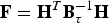 in (2) is assumed to be non-singular.
In the problem considered

It is important to stress once more that we use in (2), (3) directly measured TOAs but not calculated TDOAs because the CRLB does not depend on processing of measurements.
It is convenient to multiply time variables by the speed of light c to have all values of the same dimension. Then α = (x, y, z, c τ 0)T, and  , Bτ, and
 should be replaced by
 , Br, and
 , respectively. Equation (4) takes the form

The first three diagonal elements of Bα are variances we are interested in:  .
In certain cases spherical coordinates are more convenient to use. Then α = (R, β, ɛ, c τ 0)T and

where coordinates of the kth station are (L k, β k, ɛ k). To have all errors of the same dimension, derivatives from (3) are reasonable to be used in the form

Then the first three diagonal elements of Bα are variances of linear errors:  .
For airport surface targets, elevation angle ɛ and height z are not to be determined. In these cases, target state vectors take the form α = (x, y, c τ 0)T or α = (R, β, c τ 0)T.
III. EFFECT OF SYSTEM GEOMETRY ON POTENTIAL ACCURACY
The minimum number of stations in any MLAT system is equal to the number of unknowns of the introduced vector of state α: four (3D) or three (2D). Let us consider a ground MLAT system designed for emitter localization inside a certain area of an airport. Emitters may not be on the airport surface but their heights (or elevation angles) are not to be determined by this system. Because MLAT systems consisting of ground stations have small effective baselengthsFootnote 1 in the vertical direction with respect to ground targets, vertical PAEL for such targets is poor.
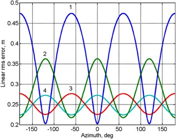
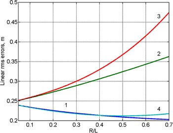
The most important problem is PAEL dependences on the number and arrangement of stations. Assume that the origin of a coordinate system is placed approximately at the center of the area. Let α = (R, β, c τ 0)T. It can be shown that the dimensionless derivatives (7) depend not on L k and R separately but on the ratio L k/R. The simplest MLAT system is a regular triangle on the horizontal plane with station coordinates, for instance (L, 0), (L, 2π/3), and (L, 4π/3). Like emitters, stations may be positioned not on the horizontal plane. Then their coordinates should be (L k, β k, ɛ k). From (2), (3), (6), and (7) we can obtain curves of PAEL shown in Figs 1 and 2. For simplicity, TOA measurement accuracy is assumed to be equal for all stations,  . In accordance with [2 − 4],
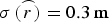 . For other values of
 (in meters), rms errors of the y-axis should be multiplied by
 .
Regular triangle. 1, 2:  and
 for R/L = 0.7; 3, 4:
 and
 for R/L = 0.2.

Regular triangle. 1, 2:  and
 for β = 0; 3, 4:
 and
 for β = 60°.

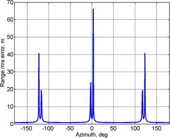
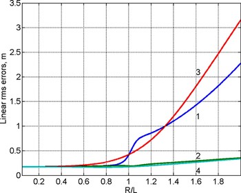
It can be seen from Figs 1 and 2 that when R approaches L, variations of errors in azimuthal directions increase significantly. Satisfactory accuracy can be obtained if R < 0.7L. For R > L, certain azimuthal directions appear where range errors grow sharply (see Fig. 3 for R/L = 1.1). It means that the Fisher information matrix is poorly conditioned in these directions. To avoid this, the number of stations should be increased. However, increasing R/L leads to a noticeable growth of range errors even for a regular hexagon (Fig. 4).
Regular triangle.  for R/L = 1.1.

Regular hexagon. 1, 2:  and
 for β = 5°; 3, 4:
 and
 for β = 30°.

Hence to obtain high PAEL in an area, it is desirable to arrange all stations enclosing this area.
It should be noted that when  , the effect of system geometry on resulting accuracy is often considered with the help of the geometric dilution of precision (GDOP) (e.g., [Reference Chernyak1, Reference Galati, Gasbarra and Leonardi2]).
 , where H1 is the same as (3) but without derivatives with respect to c τ 0 and Q is the matrix with 2 as diagonal elements and 1 elsewhere. However, we assume
 , for simplicity only. PAEL analysis permits one to take into account different values of
 (see below). Besides, for system geometry optimization, even if
 , it is important to reveal the effect of geometry on errors in different coordinates separately rather than on the integral parameter GDOP.
PAEL is often important along a line, for example, along a runway. In this case it is reasonable to use (5) instead of (6).
IV. PAEL FOR THE MLAT SYSTEM OF THE MARCO POLO AIRPORT IN VENICE, ITALY
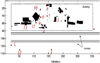
It is interesting to apply PAEL determination to a specific MLAT system. Figure 5 presents station positions of the MLAT system proposed for the Marco Polo airport in Venice, Italy [Reference Galati3].
The Marco Polo airport layout (borrowed from [Reference Galati3]).

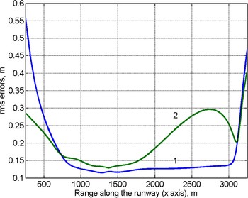
The airport surface is divided into cells approximately 10 m × 10 m, so that the x and y coordinates of each point are determined by multiplying cell indexes by 10 m. The heights of all 14 stations (in meters) are as follows: 2, 5, 2, 13, 5, 17, 5, 13, 13, 5, 17, 2, 40, and 3. In Fig. 6 PAEL [minimum attainable rms errors  and
 ] is shown for an aircraft on the runway y = 850 m. All the 14 stations are assumed to measure TOAs with an equal rms error of 1 ns. The target height is 7 m.
The Marco Polo airport, the first runway. 1:  ; 2:
 .

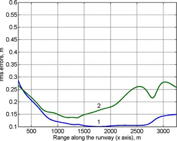
Using PAEL makes it easy to analyze the effect of changing system geometry on resulting errors. For example, placing stations No. 5 and No. 7 from Fig. 5 at the points x 5 = 2750 m, y 5 = 700 m, x 7 = 2000 m, y 7 = 550 m, and moving stations No. 1 and No. 2 along the x-axis to x 1 = 0, x 2 = 3500 m yields a certain reduction of  and
 (compare Fig. 7 with Fig. 6). PAEL in the central part of the airport does not increase noticeably. Of course, the absence of shadowing should be checked for such configuration.
1:  ; 2:
 for the same system as in Fig. 6 but with changed positions of stations 1, 2, 5, 7.

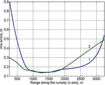
It is also easy to reveal accuracy loss caused by failures of one or several stations. Figure 8 demonstrates the increase of  and
 along the first runway in Fig. 5 when stations No. 1 and No. 2 fail to measure signal TOAs.
The same as in Fig. 6 but stations No. 1 and No. 2 do not work. 1:  ; 2:
 .

V. WAM SYSTEMS
Obviously, PMSRSs may be used not only for A-SMGCSs in airports. They are useful in air traffic control (ATC) systems because they can determine with high accuracy all the three coordinates and velocity vectors of aircrafts [Reference Chernyak1, Reference Bezoušek, Kubeček and Štěrba10]. The most difficult (but solvable) problem for WAM systems with much larger baselengths between stations (as compared with MLAT systems in airports) is the problem of stations synchronization with a high degree of precision. PAEL is very important for WAM systems as a tool for choosing system geometry, imposing requirements on TOA measurements and synchronization accuracy.
To analyze PAEL in a certain 3D zone, spherical coordinates are convenient, and the vector of state contains four unknowns: α = (R, β, ɛ, c τ 0)T. For calculations, we shall use (2), (3), (6), and derivatives in the form of (7).
If a WAM system is an extension of an airport surface MLAT system, its zone of responsibility adjoins the airport zone. Then the typical value of elevation angle ɛ for a landing or taking-off aircraft (with respect to the center of the airport) may be assumed to be 3° [Reference Galati, Gasbarra and Leonardi2].
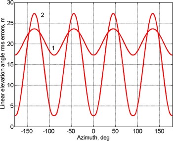
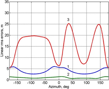
The simplest geometry of a WAM system is a three-pointed regular star. However, it cannot provide minimal localization errors simultaneously in landing and take-off directions (β near 0 and 180°). More suitable is a regular four-pointed star with β 1 = 0, β 2 = 90°, β 3 = 180°, and β 4 = 270°. It is clear that because of small ε, effective baselengths between ground stations in vertical directions are small, so that the largest errors may be expected in height (elevation angle) determination. The dependences of PAEL  on target azimuth β for R/L < 1 and R/L > 1 are presented in Fig. 9. As earlier, rms errors of TOA measurements are assumed to be 1 ns
 . It can be seen that not only larger maximum errors but also sharp variations of
 with the change of β take place when R/L increases from 0.7 to 1.2.
Regular four-pointed star ɛ = 3°;  ; 1:
 for R/L = 0.7; 2:
 for R/L = 1.2.

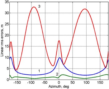
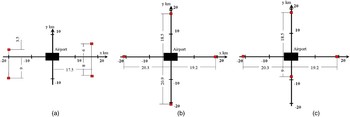
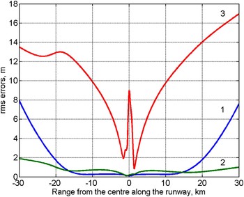
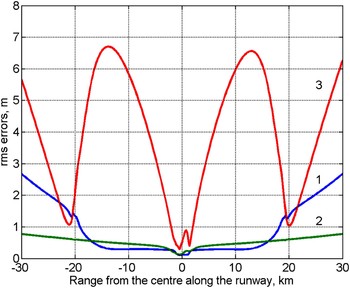
Figure 10 shows PAEL for the WAM system described in [Reference Galati, Gasbarra and Leonardi2] as an extension of the MLAT system in the Marco Polo airport. Four remote stations are added with approximate coordinates x r1 = −20 km, y r1 = 3.5 km, x r2 = 17.5 km, y r2 = 6 km, x r3 = 17.5 km, y r3 =−8 km, x r4 = −20 km, y r4 = −9 km (relative to the center of the airport, see Fig. 11(a)). TOA rms errors are as earlier 
 for 14 MLAT stations but
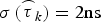
 for the remote stations [Reference Galati, Gasbarra and Leonardi2]. Target range R = 30 km. As was to be expected, potential rms errors are significantly larger than those in the MLAT system on the airport surface (see Figs 6–8).
All 14 stations of Marco Polo airport (Fig. 7) with  and four remote stations of WAM [2] with
 , ɛ = 3°, R = 30 km; 1:
 ; 2:
 ; 3:
 .

Receiver positions of the WAM system: (a) from [2], (b) after reconfiguration, and (c) after reconfiguration with limited baselength in the y direction.

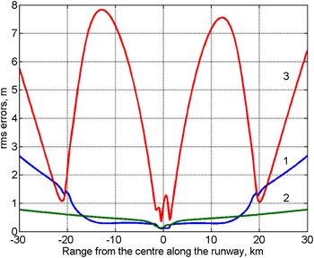
It is interesting to reveal whether it is possible to reduce errors, especially in landing and take-off directions (near 0 and 180° in azimuth), by reconfiguration of the same remote stations. Figure 12 presents PAEL for the same system as in Fig. 11(a) with the same distances of the remote stations from the center of the airport but with different directions to them. Remote stations No. 1 and No. 3 are placed along the x-axis: x r1 = −20.3 km, y r1 = 0, x r3 = 19.2 km, and y r3 = 0. Remote stations No. 2 and No. 4 are placed along the y-axis: x r2 = 0, y r2 = 18.5 km, x r4 = 0, and y r4 = −20.9 km (see Fig. 11(b)). This configuration increases effective baselengths (including vertical ones). Comparing with Fig. 10, one can see much better PAEL, especially along landing and take-off directions.
PAEL of the WAM system with the new positions of remote stations (Fig. 11(b)). 1:  ; 2:
 ; 3:
 .

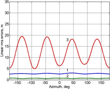
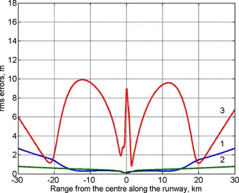
If the specific layout of the Marco Polo airport near the sea does not permit having such large distances for both remote stations along the y-axis, it may be possible at least for one station (in the mainland direction). Figure 13 shows PAEL for the same system as in Fig. 11(b) but with the y-coordinate of the fourth remote station as in [Reference Galati, Gasbarra and Leonardi2]: y r4 = −9 km (Fig. 11(c)). The better PAEL as compared with Fig. 10 is still evident.
The same as in Fig. 12 but with the new coordinates of station #4: x r4 = 0, y r4 = 9 km (Fig. 11(c)).

Figures 14 and 15 show PAEL for a landing aircraft approaching the airport from the range R = 30 km along a typical trajectory with a 3° inclination with respect to the xy plane [Reference Galati, Gasbarra and Leonardi2]. Figure 14 corresponds to the WAM system described in [Reference Galati, Gasbarra and Leonardi2]. Figure 15 stands for the system with a new arrangement of remote stations (as in Fig. 11(b)). The gain in potential accuracy is obvious.
PAEL for an approaching aircraft. WAM system from [2]; 1:  ; 2:
 ; 3:
 .

The same as in Fig. 14 but with the new positions of the remote stations as in Fig. 11(b). 1:  ; 2:
 ; 3:
 .

VI. DETERMINATION OF AIRCRAFT VELOCITY
For approaching, landing, or taking-off aircrafts, not only localization but also velocity with high accuracy is often required. The simplest way is to calculate the ratio of the coordinate estimates difference at two time moments to the time difference between these moments. For example, the estimate of velocity along the x-axis is

To increase the accuracy of  , the difference
 should be increased but if V x may be considered to be constant during this interval. Otherwise more complicated models of movement may be used, taking into account aircraft deceleration or acceleration. From the simple equation (8), the rms error of
 is

under the following natural conditions: (1) random errors of  and
 are uncorrelated, (2)
 , and (3) errors of
 may be neglected. Taking
 from PAEL calculations yields minimum attainable
 under the conditions above [or averaged
 over
 if V x is not constant during this interval].
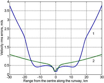
Velocity rms errors  and
 are shown in Fig. 16 for the WAM system from [Reference Galati, Gasbarra and Leonardi2] but with changed positions of remote stations as in Fig. 11(b) (the corresponding PAEL is presented in Fig. 15).
 is assumed to be 1 s. It can be seen that very high accuracy in the x direction
 remains for |x| < 15 km and sharply worsens for larger |x|. This is because the baselengths in the x direction are approximately 20 km: x r1 = −20.3 km, x r3 = 19.2 km (see Fig. 11(b)). If, for example, x r1 = −30 km, x r3 = 30 km,
 for |x| < 20 km. Height velocity is not reasonable to calculate because of insufficient PAEL in the z direction.
1:  , 2:
 for the system with PAEL from Fig. 15.

VII. INCLUDING DOA MEASUREMENTS
As mentioned in the Introduction, the concept of PAEL may be applied for systems with joint measurements of different signal parameters and target coordinates. Here we consider the WAM system for the Marco Polo airport, where receiving stations can measure not only TOAs but also DOAs. It follows from Figs 14 and 15 that the largest rms errors are in height (z) direction because of small effective baselengths in this direction. Possibly, these rms errors may be reduced by using directional antennas with not too narrow beamwidths in elevation angle direction. As far as rms errors in the x and y directions are concerned, they are small enough. Hence, on the one hand, it may not be necessary to reduce them. On the other hand, very narrow antenna beamwidths in azimuthal direction and tracking mode are required for reducing σ (x) and σ (y). Taking these difficulties into account, we assume here that a receiving station can measure not only signal TOA but also elevation angle of an emitter (relative to this station). If all stations have this feature, the extended measurement vector takes the form  while the unknown emitter's vector of state is not changed: α = (x, y, z, τ 0)T. All errors may be assumed to be uncorrelated. Then the 18 × 18 diagonal matrix Bτ in (2) should be replaced by the 36 × 36 diagonal matrix Bτɛ. In a Cartesian coordinate system,

Let us consider the WAM system for the Marco Polo airport with the earlier described new positions of remote stations (Fig. 11(b)). The PAEL along the runway for such a WAM system using only TOA measurements is presented in Fig. 15. The curves of PAEL when all 18 stations measure additionally elevation angles of an emitter with the same rms errors σ (ɛ) = 3 mrad are shown in Fig. 17.
PAEL for the WAM system with the new positions of remote stations when all stations measure signal TOAs with indicated above rms errors and emitter elevation angles with σ (ɛ) = 3 mrad. 1:  ; 2:
 ; 3:
 .

Comparing Fig. 17 with Fig. 15, one can see that the worst values of  are significantly reduced. In Fig. 18 similar curves are shown, but for the case where elevation angles can measure only nine stations: four remote stations and five stations positioned along the runway (see Fig. 5). Here
 and
 are the same as in Fig. 17 but PAEL in the z direction, as expected, becomes a little worse.

VIII. CONCLUSION
1. PAEL based on the Cramer–Rao inequality is a simple and useful tool for choosing and checking the geometry of MLAT and WAM systems as well as for imposing requirements on TOA measurement accuracy. This approach does not require a knowledge of any specific algorithm for measurement processing.
2. The effect of system geometry on PAEL is analyzed for different numbers and arrangements of receiving stations for MLAT systems. It has been shown that high PAEL (especially in range) may be obtained if a system of stations encloses the area of responsibility.
3. The concept of PAEL has been applied (as an example) to the specific MLAT and WAM systems proposed for the Marco Polo airport (Venice, Italy) [Reference Galati, Gasbarra and Leonardi2, Reference Galati3]. Certain possibilities for improving PAEL by changing the positions of stations have been revealed.
4. PAEL may be effectively used for the velocity estimation of approaching, landing, or taking-off aircrafts.
5. One of the advantages of using the concept of PAEL is the possibility to analyze the effect of joint measurements of different signal parameters and target coordinates. This was illustrated by joint measurements of signal TOAs and emitter elevation angles in the WAM system proposed for the Marco Polo airport.
 Professor Victor Chernyak received his Doctor of Science degree in 1972 and the academic rank of Professor in Radar and Radio Navigation in 1984 from the Higher Certification Commission of the USSR. From 1972 till 2001 he was with the Scientific Research Institute of Radio Device Engineering as Head of Department. Now he is a professor of two leading technical universities of Russia: Bauman Moscow State Technical University and Moscow Aviation Institute. For many years he was responsible for radar systems design, especially for signal processing and multisite (multistatic, netted) radar systems. His current research interests include signal detection and parameter estimation in multisite radar systems, wideband and ultra-wideband radars, and adaptive signal processing. Prof. Victor Chernyak is the author of more than 90 scientific papers. He is also the author of the monograph “Multisite Radar” published in 1993 in Russian. The expanded translation of this monograph into English entitled “Fundamentals of Multisite Radar Systems. Multistatic Radars and Multiradar Systems” was published by Gordon and Breach Science Publishers in 1998.
Prof. Victor Chernyak was many times invited to give lectures on radar systems in Russia and abroad including USA, France, Singapore, India, China, and Bulgaria. He is a senior member of the IEEE.