I. INTRODUCTION
Antennas have been the key element for wireless communication. The demand for multiband antenna with higher gain is increasing day-by-day for number of applications. The concept of fractalization of antenna is a good option to fulfill these needs. Fractals are self-similar geometries which may be scaled down or up with reference to its parent geometry and are followed by the repetitive pattern of the scaled geometry. Fractalization on antennas leads to multiband or wideband behavior along with the miniaturization of antenna [Reference Anguera1]. The need of proposing new fractal geometry always existed because the geometries used till now were opted either as a monopole [Reference Barroso, Mata and Diaz2], or most of the fractal geometries were used along with the coplanar wave guide (CPW) [Reference Raviteja3] or a combination of monopole with CPW [Reference Li and Mao4]. The new fractal geometries are now being used in dielectric resonator antenna [Reference Mukherjee, Patel and Mukherjee5]. All the fractal geometries used till now try to avoid the use of ground plane on the other side of the patch, i.e. below the dielectric and they do not have a good radiation property. The other way apart from exploiting the above-mentioned methods was to maintain some gap between dielectric and the ground plane [Reference Bayatmaku6]. The fractal geometries offer discontinuities thereby increasing bandwidth and resonances [Reference Wener and Ganguly7]. Several fractal geometries have been proposed and investigated in recent years including Koch, Sierpinski, Minkowski, Hilbert, and Cantor for multiband and wideband behavior. Existing fractals have numerous advantages but some of them possess limitations such as wideband behavior for a short range of frequency [Reference Pourahmadazar, Changiz and Nourinia8]. In some models, the increment in iteration results in complex geometry and coupling take place within different parts of fractal shape. It leads to shifting of resonant frequencies in higher range and performance is degraded. The proposed design has tried to overcome the above-mentioned shortcomings. In this communication, the proposed fractal antenna shows the multiband behavior with good radiation property. The new geometry is based on an iterative eight-pointed star (octagram) shape. The antenna is excited using a coax feed of 50 Ω. The basic characteristic of coax feed is narrowband [Reference Balanis9]. Therefore, use of coax feed in the proposed antenna results in multiband properties with S11 greater than −10 dB and good radiation property at the resonant frequencies.
II. ANTENNA DESIGN
In this paper, a fractal antenna is proposed implying circular-shaped substrate with feed at the center. The mentioned antenna is designed and simulated on Rogers RO4003 lossy with a dielectric constant ε
r
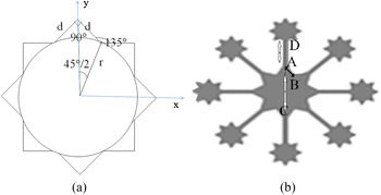
= 3.55 and the loss tangent tanδ = 0.0027. The substrate is 1.5 mm thick. The eight-pointed star shapes is a result of the combination of a central circular shape with eight triangular shapes placed at the circumference in such a way, so that edges of triangles are directly connected to each other not via circumference of the circle as shown in Fig. 1. To analyze the design of array via recursive approach [Reference Azari10], the basic eight element star shape is considered as the base or parent geometry of fractal design. The basic eight element star shape generating a sub array of
 $r = \lambda /2{\sqrt \varepsilon_r}$
, shown in Fig. 1(a) and λ = c/f, where c is the speed of light in vacuum and f is the resonant frequency of base structure. For fundamental resonant frequency of first iteration, f = 13 GHz and r = 6 mm and separation of 45° between them. Thus, we can state:
 $${\rm sin}\left( {\displaystyle{{45^\circ} \over 2}} \right) = \displaystyle{d \over r}{\rm cos}\left( {45^\circ} \right) \Rightarrow r = 1.847(d).$$
(a) Antenna geometry. (b) Second iteration.

Equation (1) gives the dimension calculation of the fractal patch; whereas equation (2) gives the array equivalent of the proposed fractal patch antenna and equations (3), and (4) describe the parameters used in mentioning the array equivalent. The array factor may be expressed as:
 $$A{F_p}(\theta ,\varphi ) = \displaystyle{1 \over {{8^p}}}\prod\limits_{p = 1}^{{8^p}} {\sum\limits_{n = 1}^8 {{e^{j\displaystyle{1 \over {{\delta ^p} - 1}}\left[ {\scriptstyle 1.847\pi \sin \theta \hfill \atop \scriptstyle \quad \cos \left( {\varphi - {\varphi _n}} \right) + {\alpha _n} \hfill} \right]}}}},$$
where
 $${\varphi _n} = \left( {n - 1} \right)\displaystyle{\pi \over 4},$$
 $${\alpha _n} = - \pi {\rm sin}{\theta _0} \cdot {\rm cos}\left( {{\varphi _0} - {\varphi _n}} \right).$$
The parameter δ is a scale factor that controls the reduction of the array of elements with each recursion and “P” is the number of iteration. Therefore, total number of radiating elements N p .
 $${N_p} = \displaystyle{8 \over 6}\left( {{7^p} - 1} \right).$$
The original fractal geometry starts with an initiator, shaped as an eight-pointed star shown in Fig. 1(a). The base model or the first iteration model has eight-pointed star patch, on a circular substrate of diameter 70 mm with a ground plane of same dimension, and feed at the center of the patch. The dimensions of the patch are AB = 4.20 mm; AC = 20.40 mm. In the first iteration, similar stars are added to the vertices of initiator star with the help of microstrip line as shown in Fig. 1(b). The same process is repeated for higher iterations. Stars added in higher iterations are scaled down copies of the initiator geometry with the scaled down factor s = 0.452 = 0.2025. The scaling is done linearly in the XY-plane by a ratio of “k”. This leads to scaling of area by a factor of “k 2”. The length of the connecting microstrip line for different iterations are AD = 12.82 and AD′ = 0.94 mm with the width of 1 and 0.5 mm for second and third iterations, respectively. The width is so adjusted that impedance is matched and maximum transfer of power takes place.
III. SIMULATION AND MEASUREMENT RESULTS
In order to assess the effectiveness as well as the reliability of the proposed designs, simulation, and numerical analysis has been carried out. The simulation has been done in the commercially available software CST Microwave Studio 2013. For simulation the transient solver has been used and the lines per wavelength were kept 10 for effective simulation.
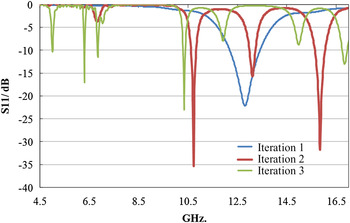
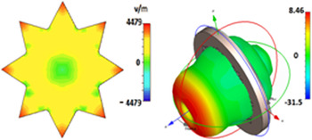
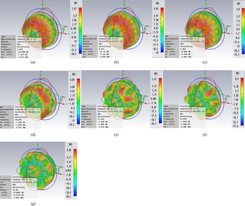
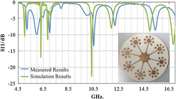
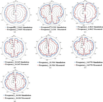
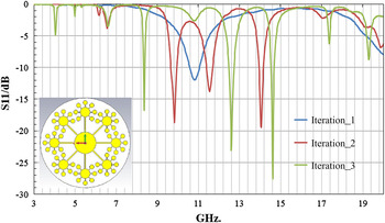
In order to investigate the effect of the different iterations of eight-pointed star fractal on the antenna performance, comparative study is done. Figure 2 shows the return loss S11/dB. Based on these results, it is observed that with every increase in iteration the number of resonant frequencies is increasing. The new incoming frequency with increased iterations follow a pattern which led us to propose a numerical method for frequency prediction of fractal geometry for higher iterations, the method is described in later section of the paper. It is clear from the comparison that because of the fractalization, the multiband behavior is taking place. The gain for the proposed antenna varies from 4.80 to 8.40 dBi for resonant frequencies. The reason for such behavior can be easily explained and analyzed using the near-field pattern of the antenna as shown in Fig. 3. From the near-field patterns, it can be concluded that the different structures for a particular iteration are behaving like an array of antenna. With addition of such elements in higher iteration, similar behavior is observed. From the radiation pattern shown in Fig. 4 it can be concluded that the radiation pattern is the pattern of the array of the antenna. The nulls at the center are due to the effective cancellation of the contributing fields of the array elements. Figures 5 and 6 show the simulation and measured S11/dB and radiation pattern of the antenna. The measured results show the close resemblance with the simulated ones.
S11 for different iterations.

Electric field pattern and the radiation pattern for first iteration at the fundamental frequency.

Radiation pattern for resonant frequencies of third iteration (a) 5.67 dBi of gain at 5.01 GHz. (b) 4.96 dBi of gain at 6.31 GHz. (c) 4.80 dBi of gain at 6.86 GHz. (d) 6.81 dBi of gain at 10.34 GHz. (e) 5.47 dBi of gain at 11.91 GHz. (f) 8.40 dBi of gain at 14.97 GHz. (g) 6.85 dBi of gain at 16.84 GHz.

S11 of simulated and fabricated antenna for third iteration.

Measured radiation pattern for resonant frequencies of third iteration (a) Measured E-plane radiation pattern at 5.01 GHz. (b) Measured E-plane radiation pattern at 6.31 GHz. (c) Measured E-plane radiation pattern at 6.86 GHz. (d) Measured E-plane radiation pattern at 10.34 GHz. (e) Measured E-plane radiation pattern at 11.91 GHz. (f) Measured E-plane radiation pattern at 14.97 GHz. (g) Measured E-plane radiation pattern at 16.84 GHz.

IV. MATHEMATICAL MODELING FOR FREQUENCY PREDICTION
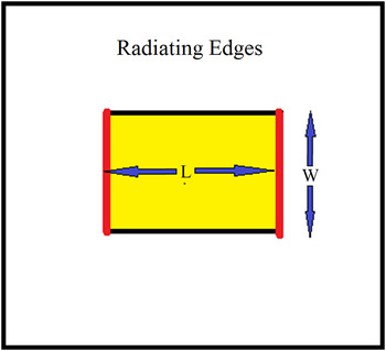
From the analysis and theory of microstrip patch antennas [Reference Balanis9]. The length “L” and width “W” of the patch of the antenna as shown in Fig. 7, are given by equations (7) and (8) for the condition given in equation (6). From equations (7) and (8) it is noticed that “L” and “W” are inversely proportional to the resonating frequency “f” of the antenna and given by equations (10) and (11). Equations (10) and (11) are multiplied and as result the equation (12) states that square of the resonating frequency is inversely proportional to the area of the patch of the microstrip patch antenna. Simplifying equation (12), it concluded that product of the square of the frequency and the area of the patch is constant for a given microstrip patch antenna. But in case of irregular shapes, the distance between the radiating edges is quite difficult to calculate. Presence of more than two edges in geometry makes it more difficult to calculate the distance between the radiating edges. Therefore, equation (14) is exploited to calculate the resonant frequency. Most of irregular shaped geometries are fractal; therefore this method is implemented for fractal antenna. Since the fundamental mode of excitation of the base structure corresponds to the single resonant frequency, after which the higher iterations are having more than one frequency so the base geometry of the first iteration is the base of our calculation. The other frequencies are calculated with the help of equation (14). The first iteration has an area of 162 mm2 corresponding to a frequency of 12.84 GHz.
 $$\displaystyle{W \over h}\rangle 1,$$
 $$w = \displaystyle{{{v_0}} \over {2f}}\sqrt {\displaystyle{2 \over {{\varepsilon _r} + 1}}}, $$
 $$L = \displaystyle{{{v_0}} \over {2f\sqrt {{\varepsilon _r}}}} - 2\Delta L,$$
 $$\Delta L = 0.412 \times h\left( {\displaystyle{{\left( {{\varepsilon _r} + 0.3} \right)\left( {W/h + 0.264} \right)} \over {\left( {{\varepsilon _r} - 0.258} \right)\left( {W/h + 0.8} \right)}}} \right),$$
 $$f \propto \displaystyle{1 \over L},$$
 $$f \propto \displaystyle{1 \over W},$$
 $${f^2} \propto \displaystyle{1 \over {L \times W}},$$
 $${f^2} \propto \displaystyle{1 \over {\rm Area}\_{\rm of}\_{\rm the}\_{\rm patch}},$$
 $${f^2} \times \hbox{Area of the patch} = {\rm constant}.$$
The patch with radiating edges separated by distance L.

First iteration in spite of being a complex geometry resonates at a single frequency, so it can be concluded that number of edges combine and form a radiating edge. So existence of “2*n” number of edges does not mean “n” number of frequency. Fractal geometry of the base structure resonating at a single frequency is considered as the base for the higher iteration calculations. Presence of single resonant frequency will correspond to the area of the smallest fractal (single element). The return loss of the antenna for simulated and fabricated antenna is shown in Fig. 5.
Example 1: The proposed star-shaped fractal antenna is taken as example 1 and the complete structure consisting of fractals which will behave like an array of antennas resonating at the same frequency with a shift in phase difference. So the contribution to the frequency will be done by the area of single antenna not the combined array. The area of fractal geometries are:
-
A = 162.00 mm2 (single element first iteration);
-
B = 32.80 mm2 (single element second iteration);
-
C = 6.64 mm2 (single element third iteration).
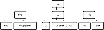
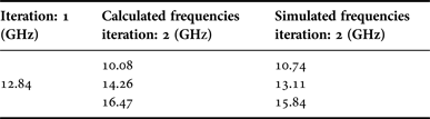
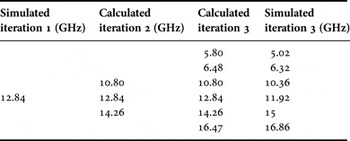
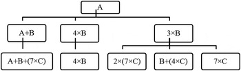
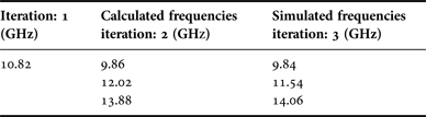
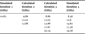
Taking first iteration to be the base of calculation and exploiting equation (14), the calculation is performed. The mentioned flow chart shown in Fig. 8 gives the schematic calculation of the resonant frequency. It also shows the areas involved for particular resonant frequency. The method proposed uses area for predicting the frequency for next iteration. The method does not deny the fundamental fact that radiation takes place from the slots of the patch. The above-mentioned flow chart shows that for second iteration the frequencies are generated because of three combinations of areas, one is from the base geometry; second, where 4–4 structures of the next iteration are excited and contribute as an array of two antennas resonating at same frequency with slight phase difference. The third frequency is generated by the excitation of 2–2 pair of structures and the antenna as a combination of two structures is resonating at the same frequency and the combined is behaving like an array of antennas. In the similar way, the frequency for next iteration can be calculated. Tables 1 and 2 show the calculated and simulated frequencies for second and third iteration of star shape fractal geometry.
Flow chart showing the generation and prediction of frequency by the use of area combination for higher iteration.

Calculated and simulated frequencies for second iteration.

Calculated and simulated frequencies for third iteration.

From equation (14) the frequencies for next iteration can be calculated. First iteration is taken as the base of the equation
First iteration:
-
• (12.84 GHz)2 × A(162.00) = Constant.
Second Iteration:
-
• (12.84 GHz)2 × A (162.00) = (x GHz)2 × (8 × B) ⇒ x = 10.80 GHz.
-
• (12.84 GHz)2 × A (162.00) = (y GHz)2 × (A) ⇒ y = 12.84 GHz.
-
• (12.84 GHz)2 × A (162.00) = (z GHz)2 × (4 × B) ⇒ z = 14.26 GHz.
Third Iteration:
-
• (12.84 GHz)2 × A (162.00) = (u GHz)2 × [A + (8 × B) + (56 × C)] ⇒ u = 5.80 GHz.
-
• (12.84 GHz)2 × A (162.00) = (v GHz)2 × [(8 × B) + (56 × C)] ⇒ v = 6.48 GHz.
-
• (12.84 GHz)2 × A (162.00) = (w GHz)2 × (8 × B) ⇒ w = 10.80 GHz
-
• (12.84 GHz)2 × A (162.00) = (x GHz)2 × (A) ⇒ x = 12.84 GHz
-
• (12.84 GHz)2 × A (162.00) = (y GHz)2 × (4 × B) ⇒ y = 14.26 GHz.
-
• (12.84 GHz)2 × A (162.00) = (z GHz)2 × (3 × B) ⇒ z = 16.47 GHz.
Example 2: Taking one more fractal geometry same as that of the star-shaped fractal geometry. The star geometries are replaced by circular patches and the areas are: A = 262.23 mm2 (single element first iteration); B = 53.10 mm2 (single element second iteration); C = 10.75 mm2 (single element third iteration). The linear scaling is 0.45 leading to (along both x & y-axis) 0.452 = 0.2025 scaling ratio in successive areas. The circular-shaped fractal geometry is shown in Fig. 9 along with S11. Taking help of equation (14) the frequencies for next iteration can be calculated for the circular-shaped fractal geometry. First iteration is taken as the base of the equation. The flow chart is shown in Fig. 10.
S11 for different iterations of second example.

Flow chart showing the generation and prediction of frequency by the use of area combination for higher iteration of second example.

First Iteration:
-
• (10.82 GHz)2 × A(262.23) = Constant.
Second Iteration:
-
• (10.82 GHz)2 × A (262.23) = (x GHz)2 × (A + B); & x = 9.86 GHz.
-
• (10.82 GHz)2 × A (262.23) = (y GHz)2 × (4 × B); & y = 12.02 GHz.
-
• (10.82 GHz)2 × A (262.23) = (z GHz)2 × (3 × B); & z = 13.88 GHz.
Third Iteration:
-
• (10.82 GHz)2 × A (262.23) = (v GHz)2 × [(A + B + (7 × C))]; & v = 8.86 GHz.
-
• (10.82 GHz)2 × A (262.23) = (w GHz)2 × (4 × B); & w = 12.02 GHz
-
• (10.82 GHz)2 × A (262.23) = (x GHz)2 × (3 × B); & x = 13.88 GHz
-
• (10.82 GHz.)2 × A (262.23) = (y GHz)2 × (B + (4 × C)); & y = 17.87 GHz.
-
• (10.82 GHz)2 × A (262.23) = (z GHz)2 × (7 × C); & z = 20.19 GHz.
V. CONCLUSION
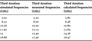
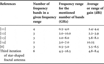
The third iteration of the proposed novel design of fractal antennas has been successively simulated and fabricated. The comparison of the S11 is shown in Fig. 5; and the mathematical modeling has been justified with one more example. Tables 3 and 4 show the simulated and calculated frequencies for higher iterations. Table 5 shows the simulated, calculated, and measured frequencies for third iteration of star-shaped fractal patch antenna. Table 6 shows the comparison of published antennas with the star shaped fractal antenna. Figure 10 gives schematic view with the help of flow chart to show the frequency prediction with the help of area calculation of different elements of different iteration.
Calculated and simulated frequencies for first iteration of second example.

Calculated and simulated frequencies for second iteration of second example.

Calculated, simulated, and measured frequencies for third iteration of first example (star-shaped fractal patch antenna).

Comparison of proposed star-shaped fractal antenna with reference antennas.

 Neeraj Rao received his Bachelor of Technology (B.Tech.) degree in Electronics and Communication Engineering from Government Engineering College, Jabalpur, India, and his Master of Technology (M.Tech.) degree in Electronics and Communication from Indian Institute of Information Technology Design and Manufacturing Jabalpur, India. He is currently pursuing his Ph.D. degree in the Department of Electronics and Communication Engineering from Indian Institute of Information Technology Design and Manufacturing Jabalpur, India. His research areas include microstrip patch antennas and fractal antennas.
 Ankit Malik received his Bachelor of Technology in 2013 in the discipline of Electronics and Communication Engineering of Pandit Dwarka Prasad Mishra (PDPM), Indian Institute of Information Technology Design and Manufacturing Jabalpur. He has worked on numerous projects on antennas and nanophotonics. He also antenna during his graduation. received medal prize for his work in fractal.
 Rahul Kumar received his B.Tech. degree (in Electronics and Communication Engineering) in 2013 from PDPM IIITDM Jabalpur. He is currently pursuing his M.Tech. in Material Physics and Engineering from National Physical Laboratory India. His research interests include plasmonics, nano-photonics, and metamaterials. He is currently working on increasing the efficiency of photo detectors using plasmonic nanostructures.
 Shobhit Goel received his B.Tech. degree in Electronics and Communication Engineering from the PDPM Indian Institute of Information Technology Design and Manufacturing, Jabalpur in 2013. Academy of Scientific and Innovative Research (AcSIR) Master degree in Advanced Material Physics and Engineering from the Council of Scientific and Industrial Research-National Physics Laboratory (CSIR-NPL), Delhi in 2015. He is currently a senior research fellow in the Department of Physics and Energy Harvesting in CSIR-NPL, India.
 Dr. Dinesh Kumar V. received his Ph.D. in Electrical Communication Engineering from Indian Institute of Science, Bangalore in 2005. He did his post-doctoral research in Japan, National Institute for Material Sciences (NIMS), Tsukuba, from November 2006 to July 2009. He became an Assistant. Professor in IIIT DM Jabalpur in 2009. He is currently serving as Associate Professor in IIIT DM Jabalpur.