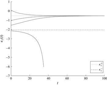
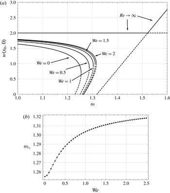
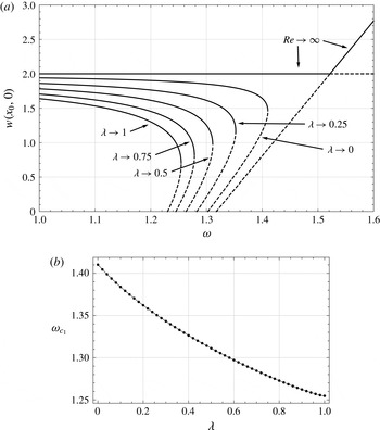
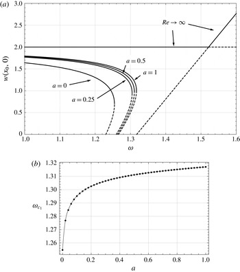
1 Introduction
Industrial apparatuses such as nozzles, hydrocyclone separators and chemical mixers use swirling flows to improve their operational performance. In some of the designs, the working fluids are non-Newtonian and exhibit viscoelastic effects. Above certain swirl levels, the rotating flows experience various instabilities, including global transition processes such as vortex breakdown phenomena. This paper concentrates on the basic interaction between inertia and viscoelasticity in a vortex flow in an open pipe and its effect on the appearance of breakdown.
Vortex breakdown is a fundamental phenomenon in fluid mechanics which refers to the significant changes in structure of swirling flows that occur above a certain level of swirl. These large-amplitude disturbances may range from weak helical waves to the stronger spiral or axisymmetric types of breakdown and change as the flow Reynolds number and swirl level are increased. Reviews of previous extensive experimental, computational and theoretical investigations of these phenomena include papers by Sarpkaya (Reference Sarpkaya1971), Hall (Reference Hall1972), Leibovich (Reference Leibovich1978, Reference Leibovich1984), Escudier (Reference Escudier1988), Althaus, Bruecker & Weimer (Reference Althaus, Bruecker and Weimer1995) and Sarpkaya (Reference Sarpkaya1995). Most studies have concentrated on the dynamics of Newtonian fluids in either vortex tubes (open pipes) or closed containers with a rotating disk. These various studies provide understanding of some aspects of the complicated transition processes. Yet, there is no consistent theoretical explanation of all of the phenomena observed.
Over the past 20 years, a theoretical framework has been developed to understand the axisymmetric vortex breakdown process and the transition to axisymmetric breakdown states in swirling flow; see Wang & Rusak (Reference Wang and Rusak1996, Reference Wang and Rusak1997a
,Reference Wang and Rusak
b
), Rusak (Reference Rusak1998), Rusak & Judd (Reference Rusak and Judd2001), Rusak et al. (Reference Rusak, Wang, Xu and Taylor2012) and Rusak, Granata & Wang (Reference Rusak, Granata and Wang2015). These authors studied the effect of increasing the swirl ratio
 $\unicode[STIX]{x1D714}$
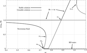
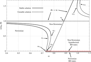
of the incoming flow to a pipe (the ratio of maximum circumferential speed to the axial speed at the vortex centreline) on the evolution to steady states in a finite-length circular pipe. A representative global bifurcation diagram of the steady-state solutions of swirling flows of an inviscid fluid and of a Newtonian fluid in a pipe of length
 $x_{0}$
and their stability characteristics are shown in figure 1. In this figure,
 $w(x_{0},0)$
is the non-dimensional centreline axial velocity at the pipe outlet, which is a representative parameter of the solution and is shown as a function of
 $\unicode[STIX]{x1D714}$
. For a base inviscid columnar (parallel) flow state,
 $w(x_{0},0)$
equals one, and this state is a solution of the inviscid flow equations for all
 $\unicode[STIX]{x1D714}$
. At certain swirl ratios, breakdown states appear, and for these states
 $w(x_{0},0)\leqslant 0$
(a reversed flow region around the centre line appears in the flow).
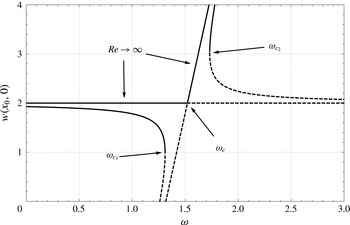
A representative global bifurcation diagram of axisymmetric steady-state solutions of swirling flows of an inviscid fluid and a Newtonian fluid and their stability characteristics. Here,
 $Re$
is the Reynolds number,
 $\unicode[STIX]{x1D714}_{c}$
is the inviscid critical swirl,
 $\unicode[STIX]{x1D714}_{c\unicode[STIX]{x1D708}1}$
and
 $\unicode[STIX]{x1D714}_{c\unicode[STIX]{x1D708}2}$
are the modified critical swirl levels due to viscosity, and
 $\unicode[STIX]{x1D714}_{0}$
and
 $\unicode[STIX]{x1D714}_{0\unicode[STIX]{x1D708}}$
are the first swirl levels for the appearance of inviscid and viscous vortex breakdown states. BD is breakdown.

The analysis of Wang & Rusak (Reference Wang and Rusak1997a
) showed that in an inviscid and axisymmetric swirling flow, there exist two critical swirl ratios,
 $\unicode[STIX]{x1D714}_{0}$
and
 $\unicode[STIX]{x1D714}_{c}$
, where
 $\unicode[STIX]{x1D714}_{0}<\unicode[STIX]{x1D714}_{c}$
(see figure 1). These critical swirls are connected by various branches of solutions. The critical swirl
 $\unicode[STIX]{x1D714}_{c}$
is a transcritical bifurcation state along the branch of columnar (parallel) flow solutions from which non-columnar (perturbed columnar) solitary-wave states bifurcate with
 $w(x_{0},0)$
decreasing from 1 to 0 as
 $\unicode[STIX]{x1D714}$
is decreased from
 $\unicode[STIX]{x1D714}_{c}$
to
 $\unicode[STIX]{x1D714}_{0}$
. The critical swirl level
 $\unicode[STIX]{x1D714}_{0}$
is a limit point of solutions from which steady breakdown states bifurcate as
 $\unicode[STIX]{x1D714}$
increases above
 $\unicode[STIX]{x1D714}_{0}$
. Moreover, it was found that axisymmetric columnar (parallel) vortex flows with swirl ratio
 $\unicode[STIX]{x1D714}$
below
 $\unicode[STIX]{x1D714}_{0}$
are asymptotically stable to any finite-size axisymmetric disturbance. When
 $\unicode[STIX]{x1D714}_{0}<\unicode[STIX]{x1D714}<\unicode[STIX]{x1D714}_{c}$
, the columnar flows are linearly stable to small disturbances, but lose their stability margin as
 $\unicode[STIX]{x1D714}$
increases towards
 $\unicode[STIX]{x1D714}_{c}$
. Furthermore, in this swirl range, sufficiently large disturbances can induce a breakdown process where the flow evolves to a lower-energy stable axisymmetric breakdown state which describes a swirling flow around a downstream-open centreline stagnation zone. When
 $\unicode[STIX]{x1D714}>\unicode[STIX]{x1D714}_{c}$
, the columnar vortex states are unstable to a certain mode of axisymmetric disturbance and the flow always evolves to a breakdown state. These instabilities are a result of the interaction between swirl-driven perturbations that tend to move upstream and the relatively fixed incoming axial and circumferential flow conditions at the pipe inlet which are imposed by the continuous operation of the vortex generator ahead of the pipe. This interaction induces a dynamic axial inhomogeneity on the flow along the pipe, which results in the appearance of large changes with increase of the swirl level.
The swirl ratio
 $\unicode[STIX]{x1D714}_{c}$
is the swirl level where a critical balance between infinitesimally small perturbations and the inlet conditions exists, and
 $\unicode[STIX]{x1D714}>\unicode[STIX]{x1D714}_{c}$
is a sufficient condition for vortex breakdown. The swirl ratio
 $\unicode[STIX]{x1D714}_{0}$
is another swirl level where a critical balance between large-amplitude disturbances and the inlet conditions can exist, and
 $\unicode[STIX]{x1D714}>\unicode[STIX]{x1D714}_{0}$
is a necessary condition for the appearance of axisymmetric breakdown in a high-Reynolds-number vortex flow. These special stability characteristics of inviscid swirling flows nicely match the results of numerical simulations according to the unsteady Euler equations (see Rusak et al.
Reference Rusak, Wang, Xu and Taylor2012 and Rusak et al.
Reference Rusak, Granata and Wang2015).
The effect of viscosity of a Newtonian fluid on the flow behaviour in an open pipe was studied in Wang & Rusak (Reference Wang and Rusak1997b
) and Rusak et al. (Reference Rusak, Granata and Wang2015). An asymptotic analysis of the Navier–Stokes equations for high-Reynolds-number (the Reynolds number,
 $Re$
, is based on the characteristic incoming axial velocity and pipe radius) flows was derived. It was found that when
 $Re$
is sufficiently high, there are two limit swirl levels,
 $\unicode[STIX]{x1D714}_{c\unicode[STIX]{x1D708}1}=\unicode[STIX]{x1D714}_{c}-C/\sqrt{Re}$
and
 $\unicode[STIX]{x1D714}_{c\unicode[STIX]{x1D708}2}=\unicode[STIX]{x1D714}_{c}+C/\sqrt{Re}$
, where equilibrium solutions of the Navier–Stokes equations fold (see again figure 1). Here,
 $C$
is a constant which depends on the inlet flow profiles. The limit level
 $\unicode[STIX]{x1D714}_{c\unicode[STIX]{x1D708}1}$
is the viscous correction to the inviscid critical swirl
 $\unicode[STIX]{x1D714}_{c}$
and increases with increase of
 $Re$
, while
 $\unicode[STIX]{x1D714}_{c\unicode[STIX]{x1D708}2}$
decreases with
 $Re$
. Similarly,
 $\unicode[STIX]{x1D714}_{0\unicode[STIX]{x1D708}}$
is the viscous correction to the inviscid critical swirl
 $\unicode[STIX]{x1D714}_{0}$
and slightly decreases towards
 $\unicode[STIX]{x1D714}_{0}$
with increase of
 $Re$
. When
 $0\leqslant \unicode[STIX]{x1D714}<\unicode[STIX]{x1D714}_{0\unicode[STIX]{x1D708}}$
, only a near-columnar stable state with
 $w(x_{0},0)$
slightly below one exists. However, when
 $\unicode[STIX]{x1D714}_{0\unicode[STIX]{x1D708}}<\unicode[STIX]{x1D714}<\unicode[STIX]{x1D714}_{c\unicode[STIX]{x1D708}1}$
, both steady near-columnar and axisymmetric breakdown states (with
 $w(x_{0},0)\leqslant 0$
) may co-exist, connected by a branch of unstable large-amplitude waves that folds back. Then, the flow evolution is determined by the initial perturbations. No near-columnar state can exist when
 $\unicode[STIX]{x1D714}_{c\unicode[STIX]{x1D708}1}<\unicode[STIX]{x1D714}<\unicode[STIX]{x1D714}_{c\unicode[STIX]{x1D708}2}$
, and, in this range of swirl, the flow must develop large-amplitude perturbations and a transition process to a breakdown state. When
 $\unicode[STIX]{x1D714}>\unicode[STIX]{x1D714}_{c\unicode[STIX]{x1D708}2}$
, the near-columnar state is unstable and the flow may evolve into either a breakdown state with
 $w(x_{0},0)\leqslant 0$
or an asymptotically stable state with an accelerated flow around the centreline and with
 $w(x_{0},0)>1$
. It was also found that when
 $Re$
is below a limit value
 $Re_{limit}$
(which also depends on the inlet flow profiles), the special fold behaviour of solutions changes. Then, only one state may exist, where a steady and stable disturbance to a columnar state grows as the swirl level is increased. These theoretical predictions for swirling flows of a Newtonian fluid nicely match the results of numerical simulations of the flow dynamics in a pipe according to the Navier–Stokes equations described in Beran & Culick (Reference Beran and Culick1992), Beran (Reference Beran1994), Lopez (Reference Lopez1994), Darmofal (Reference Darmofal1996) and Rusak et al. (Reference Rusak, Granata and Wang2015). Moreover, the experimental vortex breakdown studies of Malkiel et al. (Reference Malkiel, Cohen, Rusak and Wang1996) and Mattner, Joubert & Chong (Reference Mattner, Joubert and Chong2002) demonstrate a nice agreement of the theoretically predicted behaviour with the measured data (see also Rusak & Lamb Reference Rusak and Lamb1999).
The study of the breakdown of vortex flows of non-Newtonian fluids has concentrated on experimental investigations and numerical simulations of rotating flows in a closed container with a rotating disk (see, for example, Hill, Huppler & Bird Reference Hill, Huppler and Bird1966; Chiao & Chang Reference Chiao and Chang1990; Bohme, Rubart & Stenger Reference Bohme, Rubart and Stenger1992; Day et al. Reference Day, Harris, Soria, Boger and Welsh1996; Escudier & Cullen Reference Escudier and Cullen1996; Stokes, Lawson & Boger Reference Stokes, Graham, Lawson and Boger2001). The experiments show that the fluid viscoelasticty affects the conditions for the first appearance of vortex breakdown states, relative to those of a Newtonian fluid. Typically, it is found that the critical swirl level for breakdown increases with an increase in the shear-thinning behaviour of the liquids (Bohme et al. Reference Bohme, Rubart and Stenger1992; Escudier & Cullen Reference Escudier and Cullen1996). It should be noted, however, that most viscoelastic fluids exhibit strong shear thinning of viscosity in addition to elastic effects, and the shear-thinning effect by itself may dominate the fluid flow behaviour, increase the flow effective Reynolds number and thereby delay the appearance of vortex breakdown. Due to these separate properties, it is often difficult to interpret the physical significance of experiments, i.e. are the non-Newtonian results attributable to shear thinning or viscoelastic effects?
Among the large group of non-Newtonian fluids, Boger fluids (Boger Reference Boger1977/78; James Reference James2009) are an experimental family of fluids which consist of dilute polymer solutions generally made with a viscous solvent, for example dilute concentrations of high-molecular-weight polyacrylamide or semi-dilute concentrations of xanthan gum in a Newtonian solvent (Stokes et al.
Reference Stokes, Graham, Lawson and Boger2001). These fluids are elastic but have a nearly constant viscosity over a wide range of shear rates. Thus, they have been extensively used when isolated effects of elastic properties have been sought. Boger fluids are often modelled as the so-called Oldroyd-B fluid (Oldroyd Reference Oldroyd1950, Reference Oldroyd1958), also referred to as the upper convected Jeffreys model (Jeffreys Reference Jeffreys1929). The Oldroyd-B model is a three-parameter constitutive equation, which can be derived from the kinetic theory of solutions of elastic dumbbells, the parameters being the fluid viscosity at near-zero shear rate
 $\unicode[STIX]{x1D702}_{0}$
, relaxation time
 $\unicode[STIX]{x1D706}_{1}$
and retardation time
 $\unicode[STIX]{x1D706}_{2}$
, where both
 $\unicode[STIX]{x1D706}_{1}$
and
 $\unicode[STIX]{x1D706}_{2}$
are properties of the dissolved polymer (Bird, Armstrong & Hassager Reference Bird, Armstrong and Hassager1987a
,Reference Bird, Armstrong and Hassager
b
). The relaxation time parameter multiplies the convected time derivative of stress, while the retardation time multiplies the convected time derivative of the strain rate. The experiments of Stokes et al. (Reference Stokes, Graham, Lawson and Boger2001) demonstrate that various dilute polymer solutions are characterized by a constant
 $\unicode[STIX]{x1D706}_{1}$
and a decreasing
 $\unicode[STIX]{x1D706}_{2}$
from
 $\unicode[STIX]{x1D706}_{1}$
with the increase of polymer concentration in the Newtonian solvent.
A natural extension of the Oldroyd-B and Newtonian fluid models is possible by allowing a quadratic stress term in the constitutive equation. Giesekus (Reference Giesekus1982, Reference Giesekus1983) proposed a four-parameter model in which a constant ‘modified mobility factor’
 $a$
and the relaxation time multiply the quadratic stress term. The stress-squared term can be associated with anisotropic motion at the molecular level (Bird et al.
Reference Bird, Armstrong and Hassager1987a
,Reference Bird, Armstrong and Hassager
b
). The generalized Giesekus model also includes a term where the mobility factor and the retardation time multiply the quadratic strain term (Vlassopoulos & Hatzikiriakos Reference Vlassopoulos and Hatzikiriakos1995). This model can be derived from the kinetic theory by considering a superposition of a polymer contribution and a solvent contribution to the stress tensor (Bird et al.
Reference Bird, Armstrong and Hassager1987a
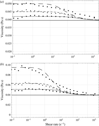
). The generalized Giesekus model can describe for the Boger fluids the realistic shear-thinning behaviour between a near-zero shear rate viscosity of the polymer plus the solvent and a high-shear-rate limit of the solvent viscosity (see the computed results in appendix A). The ratio of the retardation time to the relaxation time (
 $\unicode[STIX]{x1D706}=\unicode[STIX]{x1D706}_{2}/\unicode[STIX]{x1D706}_{1}$
) equals the ratio of solvent to fluid viscosity at near-zero shear rate. When the mobility factor
 $a$
equals zero, the Jeffreys model (Jeffreys Reference Jeffreys1929) is recovered. Increasing positive values of
 $a$
reduce the viscosity to lower values at low shear rates, thereby reducing the shear stresses. We note that the Giesekus model does not separate between shear thinning and elasticity.
The experimental studies by Stokes et al. (Reference Stokes, Graham, Lawson and Boger2001) of swirling flows of low nearly constant-viscosity Boger fluids in a container with a rotating lid have demonstrated some of the isolated effects of elasticity and its interaction with flow inertia; see table 5 and figures 19 and 20 in this reference. It was found that for a fixed geometry of the container (fixed ratio of container height to radius), decreasing the fluid retardation time
 $\unicode[STIX]{x1D706}_{2}$
with a fixed
 $\unicode[STIX]{x1D706}_{1}$
, by increasing the polymer concentration, results in an increase of the critical swirl for the first appearance of vortex breakdown above the critical swirl of the Newtonian fluid. Moreover, increasing the fluid relaxation time,
 $\unicode[STIX]{x1D706}_{1}$
(with a fixed ratio of characteristic times,
 $\unicode[STIX]{x1D706}$
), by increasing the polymer molecule size results in a decrease of the critical swirl for vortex breakdown towards the critical swirl of the Newtonian fluid. When the amount of polymer in the solvent is decreased, the two characteristic times are close to one another (
 $\unicode[STIX]{x1D706}\sim 1$
), and the fluid vortex breakdown behaviour is similar to that of a Newtonian fluid.
The effect of viscoelastic properties of fluids on the stability of vortex flows was investigated numerically by Haj-Hariri & Homsy (Reference Haj-Hariri and Homsy1997). They used an Oldroyd type model to describe the fluid stresses and studied the development of three-dimensional instabilities on the flow at the centre of a two-dimensional elliptic vortex. New modes and mechanisms of instability related to the viscous and elastic effects were in evidence. Their study was limited to vortex flows with no axial velocity, and none of the convection effects that appear when a flow in an open pipe or a container were investigated.
Review of previous works on swirling flows of non-Newtonian fluids shows that no theoretical analysis has been conducted to better understand the effects of fluid elasticity on the flow stability and the transition to breakdown. The present work extends, for the first time, the theory of vortex stability and breakdown to include effects of non-Newtonian fluids. We concentrate on the effect of fluid elasticity and shear thinning on incompressible high-Reynolds-number (
 $Re\gg 1$
) near-critical swirling flows (
 $\unicode[STIX]{x1D714}\sim \unicode[STIX]{x1D714}_{c}$
) in a finite-length straight circular open pipe. We focus on fluids where the Weissenberg number (
 $We$
) is of the order of one or less. In such cases, the elasticity number
 $El=We/Re$
is small. The stresses of the viscoelastic fluid are described by the Giesekus constitutive model to account for the effects of shear thinning and elasticity. We use the Boger fluid properties in the experiments by Stokes et al. (Reference Stokes, Graham, Lawson and Boger2001) as a reference point for viscoelastic fluid parameter values, i.e.
 $Re\sim O(1000)$
,
 $We\sim O(1)$
,
 $0<\unicode[STIX]{x1D706}<1$
and
 $a$
is small. We first apply the Giesekus model to columnar streamwise vortices and present the effect of parameter values on the base flow stress behaviour. Then, based on the limit assumptions, a nonlinear small-disturbance analysis is developed from the governing equations of motion in order to explore the complicated interactions between flow inertia, fluid viscosity, shear thinning and elasticity. The effects of changing the Reynolds number
 $Re$
, the Weissenberg number
 $We$
, the ratio of characteristic viscoelastic times
 $\unicode[STIX]{x1D706}$
and the fluid mobility
 $a$
on the flow development in the pipe and the critical swirl for vortex breakdown are explored. The present results may shed light on the changes in the appearance of breakdown zones as a function of swirl level that have been observed in the Boger fluid experiments of Stokes et al. (Reference Stokes, Graham, Lawson and Boger2001).
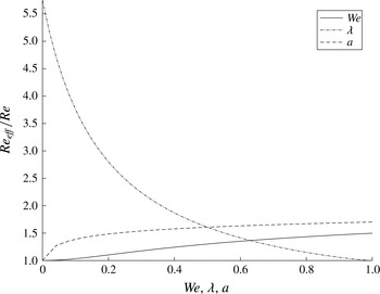
Although the present study uses the Giesekus model, it should be clarified that the analysis is not limited to the use of this constitutive model. The asymptotic model problem derived from the equations of motion of any fluid is general, and can be used with any other model that describes the stresses of a viscoelastic flow in terms of the incoming axial and circumferential velocity fields to the pipe. Specifically, the present analysis reveals, for the same inlet profiles of the axial and circumferential velocities, an effective Reynolds number that links between steady states of swirling flows of a viscoelastic fluid and those of a Newtonian fluid.
2 Mathematical model
2.1 Model equations
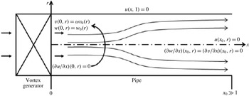
An unsteady and axisymmetric flow of an incompressible viscoelastic fluid with swirl is considered in a finite-length straight circular pipe of radius
 $R$
and length
 $\bar{x}_{0}$
(see figure 2). The pipe centreline is along the
 $\bar{x}$
axis, where
 $\bar{x}$
is the axial distance from the inlet and
 $0\leqslant \bar{x}\leqslant \bar{x}_{0}$
,
 $\unicode[STIX]{x1D703}$
is the circumferential angle
 $(0\leqslant \unicode[STIX]{x1D703}<2\unicode[STIX]{x03C0})$
and
 $\bar{r}$
is the radial distance from the centreline, where
 $0\leqslant \bar{r}\leqslant R$
. The radial, circumferential and axial components of the velocity vector
 $\bar{\boldsymbol{V}}$
are
 $\bar{u},\bar{v}$
and
 $\bar{w}$
respectively. The constant density of the fluid is
 $\bar{\unicode[STIX]{x1D70C}}$
, the pressure gauge from a reference pressure is
 $\bar{p}$
and the Cauchy stresses are
 $\bar{\unicode[STIX]{x1D70E}}_{ij}$
, where the indices
 $i$
and
 $j$
are
 $\bar{x}$
,
 $\unicode[STIX]{x1D703}$
or
 $\bar{r}$
, and
 $\bar{\unicode[STIX]{x1D70E}}_{ij}=\bar{\unicode[STIX]{x1D70E}}_{ji}$
(a symmetric stress tensor). The continuity and linear momentum equations that describe the fluid axisymmetric motion are given in a cylindrical coordinate system by
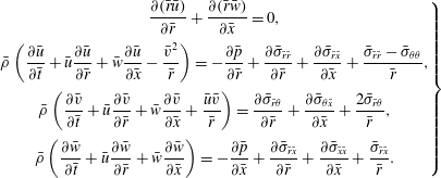 $$\begin{eqnarray}\displaystyle \left.\begin{array}{@{}c@{}}\displaystyle \frac{\unicode[STIX]{x2202}(\bar{r}\bar{u})}{\unicode[STIX]{x2202}\bar{r}}+\frac{\unicode[STIX]{x2202}(\bar{r}\bar{w})}{\unicode[STIX]{x2202}\bar{x}}=0,\\ \displaystyle \bar{\unicode[STIX]{x1D70C}}\left(\frac{\unicode[STIX]{x2202}\bar{u}}{\unicode[STIX]{x2202}\bar{t}}+\bar{u}\frac{\unicode[STIX]{x2202}\bar{u}}{\unicode[STIX]{x2202}\bar{r}}+\bar{w}\frac{\unicode[STIX]{x2202}\bar{u}}{\unicode[STIX]{x2202}\bar{x}}-\frac{\bar{v}^{2}}{\bar{r}}\right)=-\frac{\unicode[STIX]{x2202}\bar{p}}{\unicode[STIX]{x2202}\bar{r}}+\frac{\unicode[STIX]{x2202}\bar{\unicode[STIX]{x1D70E}}_{\bar{r}\bar{r}}}{\unicode[STIX]{x2202}\bar{r}}+\frac{\unicode[STIX]{x2202}\bar{\unicode[STIX]{x1D70E}}_{\bar{r}\bar{x}}}{\unicode[STIX]{x2202}\bar{x}}+\frac{\bar{\unicode[STIX]{x1D70E}}_{\bar{r}\bar{r}}-\bar{\unicode[STIX]{x1D70E}}_{\unicode[STIX]{x1D703}\unicode[STIX]{x1D703}}}{\bar{r}},\\ \displaystyle \bar{\unicode[STIX]{x1D70C}}\left(\frac{\unicode[STIX]{x2202}\bar{v}}{\unicode[STIX]{x2202}\bar{t}}+\bar{u}\frac{\unicode[STIX]{x2202}\bar{v}}{\unicode[STIX]{x2202}\bar{r}}+\bar{w}\frac{\unicode[STIX]{x2202}\bar{v}}{\unicode[STIX]{x2202}\bar{x}}+\frac{\bar{u}\bar{v}}{\bar{r}}\right)=\frac{\unicode[STIX]{x2202}\bar{\unicode[STIX]{x1D70E}}_{\bar{r}\unicode[STIX]{x1D703}}}{\unicode[STIX]{x2202}\bar{r}}+\frac{\unicode[STIX]{x2202}\bar{\unicode[STIX]{x1D70E}}_{\unicode[STIX]{x1D703}\bar{x}}}{\unicode[STIX]{x2202}\bar{x}}+\frac{2\bar{\unicode[STIX]{x1D70E}}_{\bar{r}\unicode[STIX]{x1D703}}}{\bar{r}},\\ \displaystyle \bar{\unicode[STIX]{x1D70C}}\left(\frac{\unicode[STIX]{x2202}\bar{w}}{\unicode[STIX]{x2202}\bar{t}}+\bar{u}\frac{\unicode[STIX]{x2202}\bar{w}}{\unicode[STIX]{x2202}\bar{r}}+\bar{w}\frac{\unicode[STIX]{x2202}\bar{w}}{\unicode[STIX]{x2202}\bar{x}}\right)=-\frac{\unicode[STIX]{x2202}\bar{p}}{\unicode[STIX]{x2202}\bar{x}}+\frac{\unicode[STIX]{x2202}\bar{\unicode[STIX]{x1D70E}}_{\bar{r}\bar{x}}}{\unicode[STIX]{x2202}\bar{r}}+\frac{\unicode[STIX]{x2202}\bar{\unicode[STIX]{x1D70E}}_{\bar{x}\bar{x}}}{\unicode[STIX]{x2202}\bar{x}}+\frac{\bar{\unicode[STIX]{x1D70E}}_{\bar{r}\bar{x}}}{\bar{r}}.\end{array}\right\} & & \displaystyle\end{eqnarray}$$
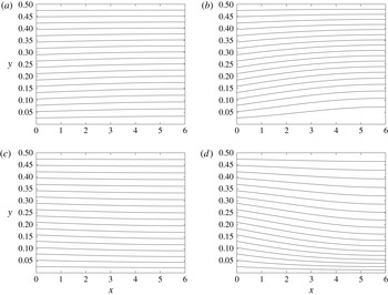
Schematic diagram of a viscous swirling flow in an open pipe.

The stress tensor
 $\bar{\unicode[STIX]{x1D70E}}$
of the viscoelastic fluid is described by the generalized Giesekus constitutive model (Bird et al.
Reference Bird, Armstrong and Hassager1987a
),
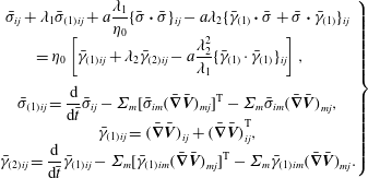 $$\begin{eqnarray}\displaystyle \left.\begin{array}{@{}c@{}}\displaystyle \bar{\unicode[STIX]{x1D70E}}_{ij}+\unicode[STIX]{x1D706}_{1}\bar{\unicode[STIX]{x1D70E}}_{(1)ij}+a\frac{\unicode[STIX]{x1D706}_{1}}{\unicode[STIX]{x1D702}_{0}}\{\bar{\unicode[STIX]{x1D70E}}\boldsymbol{\cdot }\bar{\unicode[STIX]{x1D70E}}\}_{ij}-a\unicode[STIX]{x1D706}_{2}\{\bar{\unicode[STIX]{x1D6FE}}_{(1)}\boldsymbol{\cdot }\bar{\unicode[STIX]{x1D70E}}+\bar{\unicode[STIX]{x1D70E}}\boldsymbol{\cdot }\bar{\unicode[STIX]{x1D6FE}}_{(1)}\}_{ij}\\ =\displaystyle \unicode[STIX]{x1D702}_{0}\left[\bar{\unicode[STIX]{x1D6FE}}_{(1)ij}+\unicode[STIX]{x1D706}_{2}\bar{\unicode[STIX]{x1D6FE}}_{(2)ij}-a\frac{\unicode[STIX]{x1D706}_{2}^{2}}{\unicode[STIX]{x1D706}_{1}}\{\bar{\unicode[STIX]{x1D6FE}}_{(1)}\cdot \bar{\unicode[STIX]{x1D6FE}}_{(1)}\}_{ij}\right],\quad \\ \displaystyle \bar{\unicode[STIX]{x1D70E}}_{(1)ij}=\frac{\text{d}}{\text{d}\bar{t}}\bar{\unicode[STIX]{x1D70E}}_{ij}-\unicode[STIX]{x1D6F4}_{m}[\bar{\unicode[STIX]{x1D70E}}_{im}(\bar{\unicode[STIX]{x1D735}}\bar{\boldsymbol{V}})_{mj}]^{\text{T}}-\unicode[STIX]{x1D6F4}_{m}\bar{\unicode[STIX]{x1D70E}}_{im}(\bar{\unicode[STIX]{x1D735}}\bar{\boldsymbol{V}})_{mj},\\ \displaystyle \bar{\unicode[STIX]{x1D6FE}}_{(1)ij}=(\bar{\unicode[STIX]{x1D735}}\bar{\boldsymbol{V}})_{ij}+(\bar{\unicode[STIX]{x1D735}}\bar{\boldsymbol{V}})_{ij}^{\text{T}},\\ \displaystyle \bar{\unicode[STIX]{x1D6FE}}_{(2)ij}=\frac{\text{d}}{\text{d}\bar{t}}\bar{\unicode[STIX]{x1D6FE}}_{(1)ij}-\unicode[STIX]{x1D6F4}_{m}[\bar{\unicode[STIX]{x1D6FE}}_{(1)im}(\bar{\unicode[STIX]{x1D735}}\bar{\boldsymbol{V}})_{mj}]^{\text{T}}-\unicode[STIX]{x1D6F4}_{m}\bar{\unicode[STIX]{x1D6FE}}_{(1)im}(\bar{\unicode[STIX]{x1D735}}\bar{\boldsymbol{V}})_{mj}.\end{array}\right\} & & \displaystyle\end{eqnarray}$$
Here,
 $\text{d}()/\text{d}\bar{t}=\unicode[STIX]{x2202}()/\unicode[STIX]{x2202}\bar{t}+\bar{\boldsymbol{V}}\boldsymbol{\cdot }\bar{\unicode[STIX]{x1D735}}()$
denotes the substantial derivative of a certain property and
 $\bar{\unicode[STIX]{x1D735}}\bar{\boldsymbol{V}}$
is the second-order tensor of the spatial velocity variations. Moreover,
 $\bar{\unicode[STIX]{x1D6FE}}_{(1)}$
is the rate-of-strain tensor and
 $\bar{\unicode[STIX]{x1D70E}}_{(1)ij}$
and
 $\bar{\unicode[STIX]{x1D6FE}}_{(2)ij}$
denote the contravariant convected derivatives of the extra stress
 $\bar{\unicode[STIX]{x1D70E}}$
and rate-of-strain
 $\bar{\unicode[STIX]{x1D6FE}}_{(1)}$
second-order tensors respectively. The viscosity parameter of the fluid is
 $\unicode[STIX]{x1D702}_{0}=\unicode[STIX]{x1D702}_{s}+\unicode[STIX]{x1D702}_{p}$
, where
 $\unicode[STIX]{x1D702}_{s}$
is the Newtonian solvent viscosity and
 $\unicode[STIX]{x1D702}_{p}$
is the added polymer viscosity. The constant
 $\unicode[STIX]{x1D706}_{1}$
represents the fluid relaxation time,
 $\unicode[STIX]{x1D706}_{1}\geqslant 0$
, and the constant
 $\unicode[STIX]{x1D706}_{2}$
represents the retardation time,
 $\unicode[STIX]{x1D706}_{2}\geqslant 0$
. Furthermore,
 $\unicode[STIX]{x1D702}_{0}=\unicode[STIX]{x1D702}_{s}(\unicode[STIX]{x1D706}_{1}/\unicode[STIX]{x1D706}_{2})$
. The non-dimensional constant
 $a$
is the modified mobility parameter. It should be noted that when
 $\unicode[STIX]{x1D706}_{1}=\unicode[STIX]{x1D706}_{2}=0$
, the fluid is Newtonian. When
 $\unicode[STIX]{x1D706}_{1}$
is replaced by the Maxwell relaxation time
 $\unicode[STIX]{x1D706}_{M}=\unicode[STIX]{x1D706}_{1}-\unicode[STIX]{x1D706}_{2}$
and both
 $\unicode[STIX]{x1D706}_{2}$
and
 $a$
are set to zero, the fluid is described by the generalized upper convected Maxwell model. When
 $a=0$
, the fluid is described by the Oldroyd-B model. When
 $\unicode[STIX]{x1D706}_{1}=\unicode[STIX]{x1D706}_{2}$
, the fluid behaves exactly as Newtonian. When
 $\unicode[STIX]{x1D706}_{1}=0$
and
 $\unicode[STIX]{x1D706}_{2}>0$
, the model reduces to the so-called second-order fluid (Bird et al.
Reference Bird, Armstrong and Hassager1987a
,Reference Bird, Armstrong and Hassager
b
).
In appendix A, we use the Giesekus model to calculate the stresses
 $\bar{\unicode[STIX]{x1D70E}}_{xx}$
,
 $\bar{\unicode[STIX]{x1D70E}}_{xy}$
and
 $\bar{\unicode[STIX]{x1D70E}}_{yy}$
in the case of a two-dimensional unidirectional shear flow between a stationary wall and a parallel infinite plate at distance
 $h$
moving with velocity
 $U$
in the
 $\bar{x}$
direction. The flow is in the
 $\bar{x}$
direction and the velocity components are
 $\bar{v}_{x}=\bar{\dot{\unicode[STIX]{x1D6FE}}}\bar{y}$
,
 $\bar{v}_{y}=\bar{v}_{z}=0$
, where
 $\bar{\dot{\unicode[STIX]{x1D6FE}}}=U/h$
. We demonstrate that with proper values of
 $\unicode[STIX]{x1D702}_{0}$
,
 $\unicode[STIX]{x1D706}_{1}$
,
 $\unicode[STIX]{x1D706}_{2}$
and
 $a$
, the Giesekus model may represent the nature of the fluid viscosity
 $\unicode[STIX]{x1D702}=\bar{\unicode[STIX]{x1D70E}}_{xy}/\bar{\dot{\unicode[STIX]{x1D6FE}}}$
as a function of the shear rate
 $\bar{\dot{\unicode[STIX]{x1D6FE}}}$
found in the rheological measurements of various Boger fluids shown in figure 12 of Stokes et al. (Reference Stokes, Graham, Lawson and Boger2001).
The governing equations (2.1) and (2.2) are non-dimensionalized by introducing
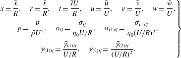 $$\begin{eqnarray}\displaystyle \left.\begin{array}{@{}c@{}}\displaystyle x=\frac{\bar{x}}{R},\quad r=\frac{\bar{r}}{R},\quad t=\frac{\bar{t}U}{R},\quad u=\frac{\bar{u}}{U},\quad v=\frac{\bar{v}}{U},\quad w=\frac{\bar{w}}{U},\\ \displaystyle p=\frac{\bar{p}}{\bar{\unicode[STIX]{x1D70C}}U^{2}},\quad \unicode[STIX]{x1D70E}_{ij}=\frac{\bar{\unicode[STIX]{x1D70E}}_{ij}}{\unicode[STIX]{x1D702}_{0}U/R},\quad \unicode[STIX]{x1D70E}_{(1)ij}=\frac{\bar{\unicode[STIX]{x1D70E}}_{(1)ij}}{\unicode[STIX]{x1D702}_{0}(U/R)^{2}},\\ \displaystyle \unicode[STIX]{x1D6FE}_{(1)ij}=\frac{\bar{\unicode[STIX]{x1D6FE}}_{(1)ij}}{U/R},\quad \unicode[STIX]{x1D6FE}_{(2)ij}=\frac{\bar{\unicode[STIX]{x1D6FE}}_{(2)ij}}{(U/R)^{2}}.\end{array}\right\} & & \displaystyle\end{eqnarray}$$
Here,
 $U$
is a characteristic speed of the incoming axial velocity to the pipe and all properties are functions of
 $x$
(
 $0\leqslant x\leqslant x_{0}$
, where
 $x_{0}=\bar{x}_{0}/R$
) and
 $r$
(
 $0\leqslant r\leqslant 1$
). Then, the continuity equation and the equations of motion (2.1) become
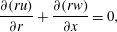 $$\begin{eqnarray}\displaystyle & \displaystyle \frac{\unicode[STIX]{x2202}(ru)}{\unicode[STIX]{x2202}r}+\frac{\unicode[STIX]{x2202}(rw)}{\unicode[STIX]{x2202}x}=0, & \displaystyle\end{eqnarray}$$
 $$\begin{eqnarray}\displaystyle & \displaystyle \frac{\unicode[STIX]{x2202}u}{\unicode[STIX]{x2202}t}+u\frac{\unicode[STIX]{x2202}u}{\unicode[STIX]{x2202}r}+w\frac{\unicode[STIX]{x2202}u}{\unicode[STIX]{x2202}x}-\frac{v^{2}}{r}=-\frac{\unicode[STIX]{x2202}p}{\unicode[STIX]{x2202}r}+\frac{1}{Re}\left(\frac{\unicode[STIX]{x2202}\unicode[STIX]{x1D70E}_{rr}}{\unicode[STIX]{x2202}r}+\frac{\unicode[STIX]{x2202}\unicode[STIX]{x1D70E}_{rx}}{\unicode[STIX]{x2202}x}+\frac{\unicode[STIX]{x1D70E}_{rr}-\unicode[STIX]{x1D70E}_{\unicode[STIX]{x1D703}\unicode[STIX]{x1D703}}}{r}\right), & \displaystyle\end{eqnarray}$$
 $$\begin{eqnarray}\displaystyle & \displaystyle \frac{\unicode[STIX]{x2202}v}{\unicode[STIX]{x2202}t}+u\frac{\unicode[STIX]{x2202}v}{\unicode[STIX]{x2202}r}+w\frac{\unicode[STIX]{x2202}v}{\unicode[STIX]{x2202}x}+\frac{uv}{r}=\frac{1}{Re}\left(\frac{\unicode[STIX]{x2202}\unicode[STIX]{x1D70E}_{r\unicode[STIX]{x1D703}}}{\unicode[STIX]{x2202}r}+\frac{\unicode[STIX]{x2202}\unicode[STIX]{x1D70E}_{\unicode[STIX]{x1D703}x}}{\unicode[STIX]{x2202}x}+\frac{2\unicode[STIX]{x1D70E}_{r\unicode[STIX]{x1D703}}}{r}\right), & \displaystyle\end{eqnarray}$$
 $$\begin{eqnarray}\displaystyle & \displaystyle \frac{\unicode[STIX]{x2202}w}{\unicode[STIX]{x2202}t}+u\frac{\unicode[STIX]{x2202}w}{\unicode[STIX]{x2202}r}+w\frac{\unicode[STIX]{x2202}w}{\unicode[STIX]{x2202}x}=-\frac{\unicode[STIX]{x2202}p}{\unicode[STIX]{x2202}x}+\frac{1}{Re}\left(\frac{\unicode[STIX]{x2202}\unicode[STIX]{x1D70E}_{xr}}{\unicode[STIX]{x2202}r}+\frac{\unicode[STIX]{x2202}\unicode[STIX]{x1D70E}_{xx}}{\unicode[STIX]{x2202}x}+\frac{\unicode[STIX]{x1D70E}_{xr}}{r}\right) & \displaystyle\end{eqnarray}$$
and the Giesekus constitutive model equation (2.2) becomes
 $$\begin{eqnarray}\displaystyle & & \displaystyle \displaystyle \unicode[STIX]{x1D70E}_{ij}+We\,\unicode[STIX]{x1D70E}_{(1)ij}+a\,We\{\unicode[STIX]{x1D70E}\cdot \unicode[STIX]{x1D70E}\}_{ij}-a\unicode[STIX]{x1D706}\,We\{\unicode[STIX]{x1D6FE}_{(1)}\cdot \unicode[STIX]{x1D70E}+\unicode[STIX]{x1D70E}\cdot \unicode[STIX]{x1D6FE}_{(1)}\}_{ij}\nonumber\\ \displaystyle & & \displaystyle \quad =\unicode[STIX]{x1D6FE}_{(1)ij}+\unicode[STIX]{x1D706}\,We\,\unicode[STIX]{x1D6FE}_{(2)ij}-a\unicode[STIX]{x1D706}^{2}\,We\{\unicode[STIX]{x1D6FE}_{(1)}\cdot \unicode[STIX]{x1D6FE}_{(1)}\}_{ij}.\end{eqnarray}$$
Here, the Reynolds number
 $Re$
, the Weissenberg number
 $We$
and the ratio of the fluid characteristic times (the ratio of retardation time to relaxation time)
 $\unicode[STIX]{x1D706}$
are defined respectively by
 $$\begin{eqnarray}Re=\frac{\bar{\unicode[STIX]{x1D70C}}UR}{\unicode[STIX]{x1D702}_{0}},\quad We=\frac{\unicode[STIX]{x1D706}_{1}U}{R},\quad \unicode[STIX]{x1D706}=\frac{\unicode[STIX]{x1D706}_{2}}{\unicode[STIX]{x1D706}_{1}}.\end{eqnarray}$$
The inverse of the Reynolds number,
 $1/Re$
, gives a measure of the viscous effects with respect to the flow inertia. The Weissenberg number
 $We$
represents a measure of the fluid elasticity effects. Since
 $\unicode[STIX]{x1D706}=\unicode[STIX]{x1D702}_{s}/\unicode[STIX]{x1D702}_{0}$
, this parameter provides a measure of shear-thinning effects. The shear thinning is also tuned by the mobility parameter
 $a$
.
2.2 Boundary conditions
We study the viscous flow in a finite-length rotating straight circular pipe with certain conditions posed on the boundaries; see figure 1. Along the pipe inlet
 $(x=0)$
, we assume fixed profiles of the axial and circumferential velocity components and of the azimuthal vorticity
 $\unicode[STIX]{x1D701}=(\unicode[STIX]{x2202}u/\unicode[STIX]{x2202}x)-(\unicode[STIX]{x2202}w/\unicode[STIX]{x2202}r)$
, given for all
 $t>0$
by
 $$\begin{eqnarray}\displaystyle & \displaystyle w(0,r,t)=w_{0}(r),\quad v(0,r,t)=\unicode[STIX]{x1D714}v_{0}(r),\quad \unicode[STIX]{x1D701}(0,r,t)=\unicode[STIX]{x1D701}_{0}(r)\quad \text{for }0\leqslant r\leqslant 1.\qquad \qquad & \displaystyle\end{eqnarray}$$
Here,
 $\unicode[STIX]{x1D714}$
represents the swirl ratio of the incoming flow. These inlet conditions reflect an incoming flow to the pipe that is created by a vortex generator ahead of the pipe in steady and continuous operation, as found in the experimental apparatuses of Sarpkaya (Reference Sarpkaya1971, Reference Sarpkaya1995), Leibovich (Reference Leibovich1978, Reference Leibovich1984), Malkiel et al. (Reference Malkiel, Cohen, Rusak and Wang1996), Mattner et al. (Reference Mattner, Joubert and Chong2002) and Umeh et al. (Reference Umeh, Rusak, Gutmark, Villalva and Cha2010). We also consider in this paper the special case where
 $\unicode[STIX]{x1D701}_{0}(r)=-\text{d}w_{0}/\text{d}r$
, which implies a zero axial gradient of the radial velocity at the inlet, i.e. for all
 $t>0$
,
 $\unicode[STIX]{x2202}u/\unicode[STIX]{x2202}x(0,r,t)=0$
. This assumption is for simplicity and does not limit the scope of the analysis, or the results, in any substantial way. It helps to focus the analysis only on the effects of the viscoelastic stresses on the flow dynamics without mixing it with other effects related to non-zero values of
 $\unicode[STIX]{x2202}u/\unicode[STIX]{x2202}x(0,r,t)$
. Rusak (Reference Rusak1998) described how general inlet azimuthal vorticity profiles can be included in the study.
In addition, since the stresses are modelled by the differential equations (2.8), the six stresses at the inlet,
 $\unicode[STIX]{x1D70E}_{ij}(0,r,t)$
, need to be set. We assume that for all
 $t\geqslant 0$
and
 $0\leqslant r\leqslant 1$
, the six stresses are given by
 $\unicode[STIX]{x1D70E}_{ij}(0,r,t)=\unicode[STIX]{x1D70E}_{ij0}(r)$
, where
 $\unicode[STIX]{x1D70E}_{ij0}(r)$
are the six stresses of a base columnar (parallel) flow state with velocity components
 $w=w_{0}(r),v=\unicode[STIX]{x1D714}v_{0}(r)$
and
 $u=0$
. These stresses are computed in § 3.
Along the pipe centreline
 $(r=0)$
, the symmetry conditions
 $$\begin{eqnarray}\displaystyle u(x,0,t)=v(x,0,t)=0,\quad \unicode[STIX]{x1D701}(x,0,t)=0\quad \text{for }0\leqslant x\leqslant x_{0} & & \displaystyle\end{eqnarray}$$
are used for all
 $t>0$
.
We assume that the influence of the rotating pipe wall axial velocity boundary layer on the swirling flow in a finite-length pipe is small within the scope of the present analysis, and a no-penetration boundary condition along the rotating wall may be sufficient to reflect the physical situation, i.e. for all
 $t>0$
, we assume along the wall
 $(r=1)$
 $$\begin{eqnarray}\displaystyle u(x,1,t)=0,\quad v(x,1,t)=\unicode[STIX]{x1D714}v_{0}(1)\quad \text{for }0\leqslant x\leqslant x_{0}. & & \displaystyle\end{eqnarray}$$
The second condition represents the no slip of the circumferential velocity on the rotating wall. These conditions may reflect the flow behaviour in a pipe with length
 $x_{0}\ll \sqrt{Re}$
and as long as the axial velocity boundary layer remains sufficiently thin with respect to the pipe radius.
At the pipe outlet
 $(x=x_{0})$
, we assume for all
 $t>0$
zero radial velocity and zero axial gradients of the axial and circumferential velocities,
 $$\begin{eqnarray}\displaystyle & \displaystyle u(x_{0},r,t)=\frac{\unicode[STIX]{x2202}w}{\unicode[STIX]{x2202}x}(x_{0},r,t)=\frac{\unicode[STIX]{x2202}v}{\unicode[STIX]{x2202}x}(x_{0},r,t)=0\quad \text{for }0\leqslant r\leqslant 1. & \displaystyle\end{eqnarray}$$
These conditions may reflect the flow development in a pipe where the pipe non-dimensional length satisfies
 $x_{0}\gg 1$
but is sufficiently shorter than the length for a fully developed viscous flow,
 $x_{0}\ll \sqrt{Re}$
.
Similar boundary conditions on the flow were considered in the analyses of Wang & Rusak (Reference Wang and Rusak1996, Reference Wang and Rusak1997a ,Reference Wang and Rusak b ) and in the numerical simulations of Beran & Culick (Reference Beran and Culick1992), Beran (Reference Beran1994), Lopez (Reference Lopez1994), Darmofal (Reference Darmofal1996) and Rusak et al. (Reference Rusak, Granata and Wang2015) of swirling flows of a Newtonian fluid in an open pipe. These boundary conditions may also reflect the physical situation as reported in the experiments of Sarpkaya (Reference Sarpkaya1971, Reference Sarpkaya1995), Leibovich (Reference Leibovich1978, Reference Leibovich1984), Malkiel et al. (Reference Malkiel, Cohen, Rusak and Wang1996) and Mattner et al. (Reference Mattner, Joubert and Chong2002).
We emphasize that there is no symmetry between the relatively fixed inlet flow conditions (2.10) and the relatively passive outlet flow conditions (2.13) in the present flow set-up (figure 2). This asymmetry generates an active role of the inlet and outlet flow states in determining the flow structure in the pipe. It forms a dynamic axial inhomogeneity of the convective flow along the pipe which results in the appearance of large axial and radial changes of the flow structure from a parallel (or a near-parallel) flow state, specifically when the swirl is close to the critical level
 $\unicode[STIX]{x1D714}_{c}$
. The viscous diffusion effects in the bulk induce an additional axial inhomogeneity which increases the size of the flow changes. The viscoelastic flow properties are found in the present study to reduce the viscous stresses and thereby somewhat decrease the viscous diffusion effects.
Equations (2.4)–(2.8) with boundary conditions (2.10)–(2.13) present a well-defined mathematical problem to describe the development of a swirling flow of an incompressible viscoelastic fluid in a pipe for any values of the parameters
 $\unicode[STIX]{x1D714}$
,
 $x_{0}$
,
 $Re$
,
 $We$
,
 $\unicode[STIX]{x1D706}$
,
 $a$
and physically relevant profiles
 $w_{0}(r)$
and
 $v_{0}(r)$
of the incoming flow, such as the Q-vortex model (Leibovich Reference Leibovich1984). The general solution of this problem requires extensive numerical computations. In this paper, we concentrate on high-Reynolds-number flows where
 $Re\gg 1$
,
 $1\ll x_{0}\ll \sqrt{Re}$
,
 $0<We\leqslant 2.5$
, and where the swirl ratio of the incoming flow is close to the critical swirl, i.e.
 $|\unicode[STIX]{x1D714}-\unicode[STIX]{x1D714}_{c}|/\unicode[STIX]{x1D714}_{c}\ll 1$
. In this case, asymptotic analysis can be used to derive approximate solutions of the problem (2.4)–(2.13) which can shed light on the nonlinear flow behaviour, the effect of viscoelasticity parameters on the critical swirl for vortex breakdown, and the flow dynamics and transition to breakdown states in a swirling flow of a viscoelastic fluid.
3 Application of the Giesekus model to columnar streamwise vortices
We first consider a base steady state of a columnar streamwise vortex flow given by the radial, axial and circumferential velocity components
 $u=0,w=w_{0}(r),v=\unicode[STIX]{x1D714}v_{0}(r)$
respectively. It should be noted that for all
 $\unicode[STIX]{x1D714}$
and profiles
 $w_{0}$
and
 $v_{0}$
, this state is a base solution of the inviscid-limit steady flow problem (2.4)–(2.13) (when
 $Re\rightarrow \infty$
). For this state, the radial momentum equation (2.5) gives the base-state pressure distribution in terms of the circumferential velocity,
 $$\begin{eqnarray}\displaystyle & \displaystyle \frac{\text{d}p_{0}}{\text{d}r}=\frac{\unicode[STIX]{x1D714}^{2}v_{0}^{2}(r)}{r}\quad \text{or}\quad p_{0}(r)=p_{0}(0)+\unicode[STIX]{x1D714}^{2}\int _{0}^{r}\frac{v_{0}^{2}(\tilde{r})}{\tilde{r}}\,\text{d}\tilde{r}. & \displaystyle\end{eqnarray}$$
Here,
 $p_{0}(0)$
is a fixed reference pressure at the centreline of the pipe inlet. Moreover, from the constitutive model equation (2.8), we find a system of six quadratic algebraic equations for the solution of the base-state viscous stresses
 $\unicode[STIX]{x1D70E}_{ij0}(r)$
. These are given in terms of the inlet velocity profiles,
 $w_{0}(r)$
and
 $\unicode[STIX]{x1D714}v_{0}(r)$
, by
 $$\begin{eqnarray}\displaystyle & & \displaystyle \displaystyle \unicode[STIX]{x1D70E}_{rr0}+a\,We(\unicode[STIX]{x1D70E}_{rr0}^{2}+\unicode[STIX]{x1D70E}_{rx0}^{2}+\unicode[STIX]{x1D70E}_{r\unicode[STIX]{x1D703}0}^{2})-2a\unicode[STIX]{x1D706}\,We\left(\unicode[STIX]{x1D714}\left(\frac{\text{d}v_{0}}{\text{d}r}-\frac{v_{0}}{r}\right)\unicode[STIX]{x1D70E}_{r\unicode[STIX]{x1D703}0}+\frac{\text{d}w_{0}}{\text{d}r}\unicode[STIX]{x1D70E}_{rx0}\right)\nonumber\\ \displaystyle & & \displaystyle \displaystyle \quad +\,a\unicode[STIX]{x1D706}^{2}\,We\left(\unicode[STIX]{x1D714}^{2}\left(\frac{\text{d}v_{0}}{\text{d}r}-\frac{v_{0}}{r}\right)^{2}+\left(\frac{\text{d}w_{0}}{\text{d}r}\right)^{2}\right)=0,\end{eqnarray}$$
 $$\begin{eqnarray}\displaystyle & & \displaystyle \displaystyle \unicode[STIX]{x1D70E}_{rx0}-We\left(\frac{\text{d}w_{0}}{\text{d}r}\unicode[STIX]{x1D70E}_{rr0}\right)+a\,We\left(\unicode[STIX]{x1D70E}_{rr0}\unicode[STIX]{x1D70E}_{rx0}+\unicode[STIX]{x1D70E}_{rx0}\unicode[STIX]{x1D70E}_{xx0}+\unicode[STIX]{x1D70E}_{r\unicode[STIX]{x1D703}0}\unicode[STIX]{x1D70E}_{\unicode[STIX]{x1D703}x0}\right)\nonumber\\ \displaystyle & & \displaystyle \displaystyle \quad -\,a\unicode[STIX]{x1D706}\,We\left(\unicode[STIX]{x1D714}\left(\frac{\text{d}v_{0}}{\text{d}r}-\frac{v_{0}}{r}\right)\unicode[STIX]{x1D70E}_{\unicode[STIX]{x1D703}x0}+\frac{\text{d}w_{0}}{\text{d}r}\left(\unicode[STIX]{x1D70E}_{rr0}+\unicode[STIX]{x1D70E}_{xx0}\right)\right)-\frac{\text{d}w_{0}}{\text{d}r}=0,\end{eqnarray}$$
 $$\begin{eqnarray}\displaystyle & & \displaystyle \displaystyle \unicode[STIX]{x1D70E}_{r\unicode[STIX]{x1D703}0}-We\,\unicode[STIX]{x1D714}\left(\frac{\text{d}v_{0}}{\text{d}r}-\frac{v_{0}}{r}\right)\unicode[STIX]{x1D70E}_{rr0}+a\,We\left(\unicode[STIX]{x1D70E}_{rr0}\unicode[STIX]{x1D70E}_{r\unicode[STIX]{x1D703}0}+\unicode[STIX]{x1D70E}_{rx0}\unicode[STIX]{x1D70E}_{\unicode[STIX]{x1D703}x0}+\unicode[STIX]{x1D70E}_{r\unicode[STIX]{x1D703}0}\unicode[STIX]{x1D70E}_{\unicode[STIX]{x1D703}\unicode[STIX]{x1D703}0}\right)\nonumber\\ \displaystyle & & \displaystyle \displaystyle \quad -\,a\unicode[STIX]{x1D706}\,We\left(\unicode[STIX]{x1D714}\left(\frac{\text{d}v_{0}}{\text{d}r}-\frac{v_{0}}{r}\right)\left(\unicode[STIX]{x1D70E}_{rr0}+\unicode[STIX]{x1D70E}_{\unicode[STIX]{x1D703}\unicode[STIX]{x1D703}0}\right)+\frac{\text{d}w_{0}}{\text{d}r}\unicode[STIX]{x1D70E}_{\unicode[STIX]{x1D703}x0}\right)-\unicode[STIX]{x1D714}\left(\frac{\text{d}v_{0}}{\text{d}r}-\frac{v_{0}}{r}\right)=0,\end{eqnarray}$$
 $$\begin{eqnarray}\displaystyle & & \displaystyle \displaystyle \unicode[STIX]{x1D70E}_{xx0}-2\,We\frac{\text{d}w_{0}}{\text{d}r}\unicode[STIX]{x1D70E}_{rx0}+a\,We\left(\unicode[STIX]{x1D70E}_{rx0}^{2}+\unicode[STIX]{x1D70E}_{xx0}^{2}+\unicode[STIX]{x1D70E}_{\unicode[STIX]{x1D703}x0}^{2}\right)\nonumber\\ \displaystyle & & \displaystyle \displaystyle \quad -\,2a\unicode[STIX]{x1D706}\,We\frac{\text{d}w_{0}}{\text{d}r}\unicode[STIX]{x1D70E}_{rx0}+2\unicode[STIX]{x1D706}\,We\left(\frac{\text{d}w_{0}}{\text{d}r}\right)^{2}+a\unicode[STIX]{x1D706}^{2}\,We\left(\frac{\text{d}w_{0}}{\text{d}r}\right)^{2}=0,\end{eqnarray}$$
 $$\begin{eqnarray}\displaystyle & & \displaystyle \displaystyle \unicode[STIX]{x1D70E}_{\unicode[STIX]{x1D703}x0}-We\left(\frac{\text{d}w_{0}}{\text{d}r}\unicode[STIX]{x1D70E}_{r\unicode[STIX]{x1D703}0}+\unicode[STIX]{x1D714}\left(\frac{\text{d}v_{0}}{\text{d}r}-\frac{v_{0}}{r}\right)\unicode[STIX]{x1D70E}_{rx0}\right)+a\,We\left(\unicode[STIX]{x1D70E}_{rx0}\unicode[STIX]{x1D70E}_{r\unicode[STIX]{x1D703}0}+\unicode[STIX]{x1D70E}_{xx0}\unicode[STIX]{x1D70E}_{\unicode[STIX]{x1D703}x0}+\unicode[STIX]{x1D70E}_{\unicode[STIX]{x1D703}x0}\unicode[STIX]{x1D70E}_{\unicode[STIX]{x1D703}\unicode[STIX]{x1D703}0}\right)\nonumber\\ \displaystyle & & \displaystyle \displaystyle \quad -\,a\unicode[STIX]{x1D706}\,We\left(\unicode[STIX]{x1D714}\left(\frac{\text{d}v_{0}}{\text{d}r}-\frac{v_{0}}{r}\right)\unicode[STIX]{x1D70E}_{rx0}+\frac{\text{d}w_{0}}{\text{d}r}\unicode[STIX]{x1D70E}_{r\unicode[STIX]{x1D703}0}\right)+2\unicode[STIX]{x1D706}\,We~\unicode[STIX]{x1D714}\left(\frac{\text{d}v_{0}}{\text{d}r}-\frac{v_{0}}{r}\right)\frac{\text{d}w_{0}}{\text{d}r}\nonumber\\ \displaystyle & & \displaystyle \displaystyle \quad +\,a\unicode[STIX]{x1D706}^{2}\,We\,\unicode[STIX]{x1D714}\left(\frac{\text{d}v_{0}}{\text{d}r}-\frac{v_{0}}{r}\right)\frac{\text{d}w_{0}}{\text{d}r}=0,\end{eqnarray}$$
 $$\begin{eqnarray}\displaystyle & & \displaystyle \displaystyle \unicode[STIX]{x1D70E}_{\unicode[STIX]{x1D703}\unicode[STIX]{x1D703}0}-2\,We\,\unicode[STIX]{x1D714}\left(\frac{\text{d}v_{0}}{\text{d}r}-\frac{v_{0}}{r}\right)\unicode[STIX]{x1D70E}_{r\unicode[STIX]{x1D703}0}+a\,We\,\left(\unicode[STIX]{x1D70E}_{r\unicode[STIX]{x1D703}0}^{2}+\unicode[STIX]{x1D70E}_{\unicode[STIX]{x1D703}x0}^{2}+\unicode[STIX]{x1D70E}_{\unicode[STIX]{x1D703}\unicode[STIX]{x1D703}0}^{2}\right)\nonumber\\ \displaystyle & & \displaystyle \displaystyle \quad -\,2a\unicode[STIX]{x1D706}\,We\,\unicode[STIX]{x1D714}\left(\frac{\text{d}v_{0}}{\text{d}r}-\frac{v_{0}}{r}\right)\unicode[STIX]{x1D70E}_{r\unicode[STIX]{x1D703}0}+2\unicode[STIX]{x1D706}\,We\,\unicode[STIX]{x1D714}^{2}\left(\frac{\text{d}v_{0}}{\text{d}r}-\frac{v_{0}}{r}\right)^{2}\nonumber\\ \displaystyle & & \displaystyle \displaystyle \quad +\,a\unicode[STIX]{x1D706}^{2}\,We\,\unicode[STIX]{x1D714}^{2}\left(\frac{\text{d}v_{0}}{\text{d}r}-\frac{v_{0}}{r}\right)^{2}=0.\end{eqnarray}$$
When
 $a=0$
(the Oldroyd-B model) equations (3.2)–(3.7) can be solved analytically and result in
 $$\begin{eqnarray}\displaystyle & \left.\begin{array}{@{}c@{}}\displaystyle \unicode[STIX]{x1D70E}_{rr0}=0,\quad \unicode[STIX]{x1D70E}_{rx0}=\frac{\text{d}w_{0}}{\text{d}r},\quad \unicode[STIX]{x1D70E}_{r\unicode[STIX]{x1D703}0}=\unicode[STIX]{x1D714}\left(\frac{\text{d}v_{0}}{\text{d}r}-\frac{v_{0}}{r}\right),\\ \displaystyle \unicode[STIX]{x1D70E}_{xx0}=2(1-\unicode[STIX]{x1D706})We\left(\frac{\text{d}w_{0}}{\text{d}r}\right)^{2},\quad \unicode[STIX]{x1D70E}_{\unicode[STIX]{x1D703}x0}=2(1-\unicode[STIX]{x1D706})We\,\unicode[STIX]{x1D714}\left(\frac{\text{d}v_{0}}{\text{d}r}-\frac{v_{0}}{r}\right)\frac{\text{d}w_{0}}{\text{d}r},\\ \displaystyle \unicode[STIX]{x1D70E}_{\unicode[STIX]{x1D703}\unicode[STIX]{x1D703}0}=2(1-\unicode[STIX]{x1D706})We\,\unicode[STIX]{x1D714}^{2}\left(\frac{\text{d}v_{0}}{\text{d}r}-\frac{v_{0}}{r}\right)^{2}.\end{array}\right\} & \displaystyle\end{eqnarray}$$
In addition, the stresses reduce to the Newtonian fluid case when
 $\unicode[STIX]{x1D706}\rightarrow 1$
or when
 $We=0$
.
For given values of
 $\unicode[STIX]{x1D714}$
,
 $We$
,
 $\unicode[STIX]{x1D706}$
and
 $a$
and known functions
 $v_{0}(r)$
and
 $w_{0}(r)$
, the stress equations (3.2)–(3.7) are solved numerically for any
 $0\leqslant r\leqslant 1$
using an iterative root-finding procedure. We demonstrate the nature of the base stresses for the case where the incoming vortex flow is given by the streamwise Q-vortex model (defined by Leibovich Reference Leibovich1984),
 $$\begin{eqnarray}\displaystyle & \displaystyle w_{0}(r)=1+\unicode[STIX]{x1D6FF}\text{e}^{-\unicode[STIX]{x1D6FD}r^{2}},\quad v_{0}(r)=\frac{1}{r}(1-\text{e}^{-\unicode[STIX]{x1D6FD}r^{2}}). & \displaystyle\end{eqnarray}$$
Here,
 $\unicode[STIX]{x1D6FD}$
is a constant related to the vortex core radius,
 $r_{c}=1.12/\sqrt{\unicode[STIX]{x1D6FD}}$
, and
 $\unicode[STIX]{x1D6FF}$
is a parameter that characterizes the jet (
 $\unicode[STIX]{x1D6FF}>0$
) or wake (
 $\unicode[STIX]{x1D6FF}<0$
) nature of the axial velocity. The Q-vortex model may represent experimental vortex flows at the inlet of an open vortex tube when
 $\unicode[STIX]{x1D6FF}>0$
(see, for example, Leibovich Reference Leibovich1984). Of specific interest for the following analysis are the base flow shear stresses
 $\unicode[STIX]{x1D70E}_{r\unicode[STIX]{x1D703}0}(r)$
and
 $\unicode[STIX]{x1D70E}_{rx0}(r)$
.
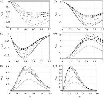
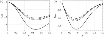
Profiles of the base flow stresses for a jet swirling flow at various Weissenberg numbers; (a)
 $\unicode[STIX]{x1D70E}_{rr0}$
, (b)
 $\unicode[STIX]{x1D70E}_{r\unicode[STIX]{x1D703}0}$
, (c)
 $\unicode[STIX]{x1D70E}_{rx0}$
, (d)
 $\unicode[STIX]{x1D70E}_{\unicode[STIX]{x1D703}\unicode[STIX]{x1D703}0}$
, (e)
 $\unicode[STIX]{x1D70E}_{\unicode[STIX]{x1D703}x0}$
, (f)
 $\unicode[STIX]{x1D70E}_{xx0}$
. The viscoelastic fluid parameter values are
 $\unicode[STIX]{x1D706}=0.5$
and
 $a=0.5$
. The parameters of the Q-vortex (3.9) are
 $\unicode[STIX]{x1D714}=1.5216$
,
 $\unicode[STIX]{x1D6FD}=4$
,
 $\unicode[STIX]{x1D6FF}=1$
; solid line, Newtonian fluid,
 $We=0$
; short dashed line,
 $We=0.1$
; intermediate dashed line,
 $We=0.2$
; long dashed line,
 $We=0.5$
; longest dashed line,
 $We=1$
; line with circles,
 $We=1.5$
; line with squares,
 $We=2$
; line with diamonds,
 $We=2.5$
.

For example, the six stresses of the viscoelastic fluid are calculated as functions of
 $r$
for a streamwise Q-vortex (3.9) with parameters
 $\unicode[STIX]{x1D6FD}=4$
,
 $\unicode[STIX]{x1D6FF}=1$
(an axial jet flow) and
 $\unicode[STIX]{x1D714}=\unicode[STIX]{x1D714}_{c}=1.5216$
. Results are shown in the six panels of figure 3 for a Newtonian fluid (
 $We=0$
, the solid line) and for representative values
 $We=0.1,0.2,0.5,1,1.5,2$
and
 $2.5$
. Here, for all stresses, the viscoelastic fluid parameters
 $\unicode[STIX]{x1D706}=0.5$
and
 $a=0.5$
are held fixed. It can be seen that the base flow stress
 $\unicode[STIX]{x1D70E}_{rr0}$
becomes negative and increases in its absolute size all across the pipe radius as
 $We$
is increased from
 $0$
to
 $0.5$
(figure 3
a). Then,
 $\unicode[STIX]{x1D70E}_{rr0}$
becomes less negative and decreases in its absolute size with further increase of
 $We$
above
 $0.5$
. The shear stresses
 $\unicode[STIX]{x1D70E}_{r\unicode[STIX]{x1D703}0}$
and
 $\unicode[STIX]{x1D70E}_{rx0}$
become less negative and decrease in their absolute values all across the pipe radius as
 $We$
is increased from
 $0$
to
 $2.5$
(figure 3
b,c). The stresses
 $\unicode[STIX]{x1D70E}_{\unicode[STIX]{x1D703}\unicode[STIX]{x1D703}0}$
and
 $\unicode[STIX]{x1D70E}_{\unicode[STIX]{x1D703}x0}$
increase in their size as
 $We$
is increased from
 $0$
to
 $0.5$
and then decrease in size with further increase of
 $We$
above
 $0.5$
(figure 3
d,e). The stress
 $\unicode[STIX]{x1D70E}_{xx0}$
increases in its size as
 $We$
is increased from
 $0$
to
 $1$
and then decreases in size with further increase of
 $We$
above
 $1$
(figure 3
f). In this case, increasing the relaxation time also increases the retardation time to keep the viscoelastic time ratio fixed.
At the given parameters, the Giesekus model shows decrease of the shear stresses
 $\unicode[STIX]{x1D70E}_{r\unicode[STIX]{x1D703}0}$
and
 $\unicode[STIX]{x1D70E}_{rx0}$
with increase of the relaxation time (fluid elasticity). However, the effect of increasing
 $We$
on the normal stresses is non-monotonic due to the highly coupled nonlinear interaction between flow strain, relaxation, retardation and mobility effects, i.e. between the elastic effects and the shear-thinning effects. When
 $0<We<0.5$
is small (very small fluid elasticity), the effect of the nonlinear terms associated with mobility and shear thinning may dominate to cause an increase in size of the normal stresses. When
 $We$
is higher, the effect of relaxation and elasticity may dominate to cause a decrease of the normal stresses. The decrease in size of the shear stresses
 $\unicode[STIX]{x1D70E}_{r\unicode[STIX]{x1D703}0}$
and
 $\unicode[STIX]{x1D70E}_{rx0}$
with the increase of
 $We$
has an effect on the swirling jet viscoelastic fluid mechanics.
Figure 4 shows the computed base flow profiles of
 $\unicode[STIX]{x1D70E}_{r\unicode[STIX]{x1D703}0}$
and
 $\unicode[STIX]{x1D70E}_{rx0}$
for various values of the characteristic time ratio
 $\unicode[STIX]{x1D706}$
between
 $0$
and
 $1$
(a Newtonian fluid behaviour) at fixed values of
 $We=1.5$
and
 $a=0.5$
. The two stresses are negative for all
 $0\leqslant r\leqslant 1$
and increase in their absolute size towards the respective Newtonian fluid stresses with increase of
 $\unicode[STIX]{x1D706}$
towards 1. In this case, the relaxation time is fixed, and by increasing
 $\unicode[STIX]{x1D706}$
, the retardation time is increased. At the given parameters, according to the Giesekus model, there is an increase of the shear stresses in absolute size with decrease in the shear-thinning effects (increase of
 $\unicode[STIX]{x1D706}$
from 0 to 1).
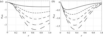
The effect of changing the mobility parameter
 $a$
from
 $0$
to
 $1$
on the base stress distribution in a streamwise Q-vortex jet flow (3.9) with
 $\unicode[STIX]{x1D6FD}=4$
,
 $\unicode[STIX]{x1D6FF}=1$
and
 $\unicode[STIX]{x1D714}=\unicode[STIX]{x1D714}_{c}=1.5216$
is shown in figure 5. Here,
 $We=1.5$
and
 $\unicode[STIX]{x1D706}=0.5$
are held fixed. It can be seen that increasing
 $a$
from
 $0$
(the Oldroyd-B model) to
 $1$
causes a decrease in the size of the stresses
 $\unicode[STIX]{x1D70E}_{r\unicode[STIX]{x1D703}0}$
and
 $\unicode[STIX]{x1D70E}_{rx0}$
all across the pipe. In this case, the relaxation and retardation times are fixed. At the given parameters, according to the Giesekus model, increasing the mobility parameter decreases the size of the shear stresses. This effect is significant specifically in the range of
 $a$
between
 $0$
and
 $0.25$
.
Profiles of the base flow stresses for a jet swirling flow at various characteristic time ratios; (a)
 $\unicode[STIX]{x1D70E}_{r\unicode[STIX]{x1D703}0}$
, (b)
 $\unicode[STIX]{x1D70E}_{rx0}$
. The viscoelastic fluid parameter values are
 $We=1.5$
and
 $a=0.5$
. The parameters of the Q-vortex (3.9) are
 $\unicode[STIX]{x1D714}=1.5216$
,
 $\unicode[STIX]{x1D6FD}=4$
,
 $\unicode[STIX]{x1D6FF}=1$
; solid line,
 $\unicode[STIX]{x1D706}=0$
; short dashed line,
 $\unicode[STIX]{x1D706}=0.25$
; intermediate dashed line,
 $\unicode[STIX]{x1D706}=0.5$
; long dashed line,
 $\unicode[STIX]{x1D706}=0.75$
; longest dashed line,
 $\unicode[STIX]{x1D706}=1$
.

Profiles of the base flow stresses for a jet swirling flow at various mobility parameter values; (a)
 $\unicode[STIX]{x1D70E}_{r\unicode[STIX]{x1D703}0}$
, (b)
 $\unicode[STIX]{x1D70E}_{rx0}$
. The viscoelastic fluid parameter values are
 $We=1.5$
and
 $\unicode[STIX]{x1D706}=0.5$
. The parameters of the Q-vortex (3.9) are
 $\unicode[STIX]{x1D714}=1.5216$
,
 $\unicode[STIX]{x1D6FD}=4$
,
 $\unicode[STIX]{x1D6FF}=1$
; solid line,
 $a=0$
; short dashed line,
 $a=0.25$
; intermediate dashed line,
 $a=0.5$
; long dashed line,
 $a=1$
.

Computations of the stresses for a base Q-vortex wake flow (3.9) with parameters
 $\unicode[STIX]{x1D6FD}=4$
,
 $\unicode[STIX]{x1D6FF}=-0.3$
and
 $\unicode[STIX]{x1D714}=\unicode[STIX]{x1D714}_{c}=0.6792$
exhibit a similar behaviour (results are not shown). It should be noted that for flows with an axial wake profile, the stress
 $\unicode[STIX]{x1D70E}_{rx0}(r)$
is positive since
 $(\text{d}w_{0}/\text{d}r)>0$
for all
 $r$
. It is found that the base flow stresses
 $\unicode[STIX]{x1D70E}_{r\unicode[STIX]{x1D703}0}$
and
 $\unicode[STIX]{x1D70E}_{rx0}$
of the viscoelastic fluid decrease in their absolute size all across the pipe radius as
 $We$
(relaxation time and fluid elasticity) is increased from
 $0$
to
 $2$
with fixed values of
 $\unicode[STIX]{x1D706}$
and
 $a$
. These stresses decrease in their size with decrease of
 $\unicode[STIX]{x1D706}$
from
 $1$
to
 $0$
(with increase of shear thinning) or increase of
 $a$
from
 $0$
(the Oldroyd-B model).
4 Small-disturbance approach
An asymptotic solution is now developed to study the equilibrium states of high-Reynolds-number near-critical swirling flows of a viscoelastic fluid.
4.1 The perturbation equations and critical swirl
It is expected that for every inlet swirl level
 $\unicode[STIX]{x1D714}$
, viscous effects of the order of
 $O(1/Re)$
create correspondingly small perturbations from the base inviscid-limit columnar flow state where
 $u=0,w=w_{0}(r),v=\unicode[STIX]{x1D714}v_{0}(r)$
. However, previous studies (Wang & Rusak Reference Wang and Rusak1997b
) have shown that near the critical swirl
 $\unicode[STIX]{x1D714}_{c}$
the velocity perturbations to a columnar flow solution of order
 $\unicode[STIX]{x1D716}_{1}$
can be much greater than
 $O(1/Re)$
. These velocity perturbations are a result of the nonlinear interaction between the near-critical level of swirl of the flow and the small viscous effects, including the viscoelastic effects. Therefore, following Wang & Rusak (Reference Wang and Rusak1997b
), we assume for all
 $t>0$
and for
 $0\leqslant x\leqslant x_{0}$
and
 $0\leqslant r\leqslant 1$
the following asymptotic expansions about the base steady inviscid-limit columnar state:
 $$\begin{eqnarray}\displaystyle & w(x,y,t)=w_{0}(r)+\unicode[STIX]{x1D716}_{1}(t)w_{1}(x,r)+\unicode[STIX]{x1D716}_{2}(t)w_{2}(x,r)+\cdots \,, & \displaystyle\end{eqnarray}$$
 $$\begin{eqnarray}\displaystyle & u(x,y,t)=\unicode[STIX]{x1D716}_{1}(t)u_{1}(x,r)+\unicode[STIX]{x1D716}_{2}u_{2}(t)(x,r)+\cdots \,, & \displaystyle\end{eqnarray}$$
 $$\begin{eqnarray}\displaystyle & v(x,y,t)=\unicode[STIX]{x1D714}v_{0}(r)+\unicode[STIX]{x1D716}_{1}(t)v_{1}(x,r)+\unicode[STIX]{x1D716}_{2}(t)v_{2}(x,r)+\cdots \,, & \displaystyle\end{eqnarray}$$
 $$\begin{eqnarray}\displaystyle & K(x,y,t)=rv=\unicode[STIX]{x1D714}K_{0}(r)+\unicode[STIX]{x1D716}_{1}(t)K_{1}(x,r)+\unicode[STIX]{x1D716}_{2}(t)K_{2}(x,r)+\cdots \,, & \displaystyle\end{eqnarray}$$
 $$\begin{eqnarray}\displaystyle & p(x,y,t)=p_{0}(r)+\unicode[STIX]{x1D716}_{1}(t)p_{1}(x,r)+\unicode[STIX]{x1D716}_{2}(t)p_{2}(x,r)+\cdots \,, & \displaystyle\end{eqnarray}$$
 $$\begin{eqnarray}\displaystyle & \unicode[STIX]{x1D70E}_{ij}(x,y,t)=\unicode[STIX]{x1D70E}_{ij0}(r)+\unicode[STIX]{x1D716}_{1}(t)\unicode[STIX]{x1D70E}_{ij1}(x,r)\cdots \quad \text{for every }i,j=r,\unicode[STIX]{x1D703},x. & \displaystyle\end{eqnarray}$$
Here,
 $K$
denotes the circulation function, with
 $K_{0}(r)=rv_{0}(r)$
. We assume that
 $|\unicode[STIX]{x1D716}_{2}|\ll |\unicode[STIX]{x1D716}_{1}|\ll 1$
,
 $|\unicode[STIX]{x1D716}_{1}|\gg 1/Re$
, and at the second-order terms
 $\unicode[STIX]{x1D716}_{2}\sim \text{d}\unicode[STIX]{x1D716}_{1}/\text{d}t,\,\sim \unicode[STIX]{x1D716}_{1}^{2}\sim 1/Re$
. (We note that assuming
 $1/Re\sim \unicode[STIX]{x1D716}_{1}$
results in a singularity and a breakdown of the above asymptotic expansions when
 $\unicode[STIX]{x1D714}$
approaches the critical level
 $\unicode[STIX]{x1D714}_{c}$
(Wang & Rusak Reference Wang and Rusak1997b
).) Moreover, it is assumed that
 $\unicode[STIX]{x1D714}=\unicode[STIX]{x1D714}_{c}+\unicode[STIX]{x0394}\unicode[STIX]{x1D714}$
, where
 $|\unicode[STIX]{x0394}\unicode[STIX]{x1D714}|/\unicode[STIX]{x1D714}_{c}\ll 1$
, and that
 $\unicode[STIX]{x1D716}_{1}$
and
 $\unicode[STIX]{x1D716}_{2}$
are functions of
 $t$
,
 $1/Re$
and
 $\unicode[STIX]{x0394}\unicode[STIX]{x1D714}$
. The base-state pressure
 $p_{0}(r)$
and viscous flow stresses
 $\unicode[STIX]{x1D70E}_{ij0}(r)$
(where
 $i,j=r,\unicode[STIX]{x1D703},x$
) are given by (3.1)–(3.7). It should be noted that when
 $We\sim O(1)$
, the terms with
 $\unicode[STIX]{x1D70E}_{ij1}(x,r)$
in (2.5)–(2.7) and in (2.8) may be neglected. These assumptions lead to the richest problem of interaction between inertia, viscosity and elasticity.
The boundary conditions (2.10)–(2.13) result in conditions on the various velocity perturbations,
 $$\begin{eqnarray}\displaystyle & \displaystyle w_{1}(0,r)=w_{2}(0,r)=v_{1}(0,r)=v_{2}(0,r)\phantom{\text{for }0\leqslant r\leqslant 1,} & \displaystyle \nonumber\\ \displaystyle & \displaystyle \phantom{w_{1}(0,r)}=\frac{\unicode[STIX]{x2202}u_{1}}{\unicode[STIX]{x2202}x}(0,r)=\frac{\unicode[STIX]{x2202}u_{2}}{\unicode[STIX]{x2202}x}(0,r)=0\quad \text{for }0\leqslant r\leqslant 1, & \displaystyle\end{eqnarray}$$
 $$\begin{eqnarray}\displaystyle & \displaystyle \frac{\unicode[STIX]{x2202}w_{1}}{\unicode[STIX]{x2202}x}(x_{0},r)=\frac{\unicode[STIX]{x2202}w_{2}}{\unicode[STIX]{x2202}x}(x_{0},r)=\frac{\unicode[STIX]{x2202}v_{1}}{\unicode[STIX]{x2202}x}(x_{0},r)=\frac{\unicode[STIX]{x2202}v_{2}}{\unicode[STIX]{x2202}x}(x_{0},r) & \displaystyle \nonumber\\ \displaystyle & \displaystyle \phantom{\frac{\unicode[STIX]{x2202}w_{1}}{\unicode[STIX]{x2202}x}(x_{0},r)==}=u_{1}(x_{0},r)=u_{2}(x_{0},r)=0\quad \text{for }0\leqslant r\leqslant 1, & \displaystyle\end{eqnarray}$$
 $$\begin{eqnarray}\displaystyle & \displaystyle u_{1}(x,0)=u_{2}(x,0)=v_{1}(x,0)=v_{2}(x,0)=0\quad \text{for }0\leqslant x\leqslant x_{0}, & \displaystyle\end{eqnarray}$$
 $$\begin{eqnarray}\displaystyle & \displaystyle u_{1}(x,1)=u_{2}(x,1)=v_{1}(x,1)=v_{2}(x,1)=0\quad \text{for }0\leqslant x\leqslant x_{0}. & \displaystyle\end{eqnarray}$$
The continuity equation (2.4) and expansions (4.1) and (4.2) give in the leading orders
 $O(\unicode[STIX]{x1D716}_{1})$
and
 $O(\unicode[STIX]{x1D716}_{2})$
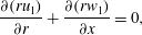 $$\begin{eqnarray}\displaystyle & \displaystyle \frac{\unicode[STIX]{x2202}(ru_{1})}{\unicode[STIX]{x2202}r}+\frac{\unicode[STIX]{x2202}(rw_{1})}{\unicode[STIX]{x2202}x}=0, & \displaystyle\end{eqnarray}$$
 $$\begin{eqnarray}\displaystyle & \displaystyle \frac{\unicode[STIX]{x2202}(ru_{2})}{\unicode[STIX]{x2202}r}+\frac{\unicode[STIX]{x2202}(rw_{2})}{\unicode[STIX]{x2202}x}=0 & \displaystyle\end{eqnarray}$$
respectively. Perturbation stream functions
 $\unicode[STIX]{x1D713}_{1}(x,r)$
and
 $\unicode[STIX]{x1D713}_{2}(x,r)$
are defined as
 $$\begin{eqnarray}\frac{\unicode[STIX]{x2202}\unicode[STIX]{x1D713}_{1}}{\unicode[STIX]{x2202}x}=-ru_{1},\quad \frac{\unicode[STIX]{x2202}\unicode[STIX]{x1D713}_{1}}{\unicode[STIX]{x2202}r}=rw_{1},\end{eqnarray}$$
 $$\begin{eqnarray}\frac{\unicode[STIX]{x2202}\unicode[STIX]{x1D713}_{2}}{\unicode[STIX]{x2202}x}=-ru_{2},\quad \frac{\unicode[STIX]{x2202}\unicode[STIX]{x1D713}_{2}}{\unicode[STIX]{x2202}r}=rw_{2}.\end{eqnarray}$$
The boundary conditions (4.7)–(4.10) provide conditions for
 $\unicode[STIX]{x1D713}_{1}$
and
 $\unicode[STIX]{x1D713}_{2}$
,
 $$\begin{eqnarray}\displaystyle & \displaystyle \unicode[STIX]{x1D713}_{1}(0,r)=\frac{\unicode[STIX]{x2202}^{2}\unicode[STIX]{x1D713}_{1}}{\unicode[STIX]{x2202}x^{2}}(0,r)=0,\quad \frac{\unicode[STIX]{x2202}\unicode[STIX]{x1D713}_{1}}{\unicode[STIX]{x2202}x}(x_{0},r)=0\quad \text{for }0\leqslant r\leqslant 1, & \displaystyle\end{eqnarray}$$
 $$\begin{eqnarray}\displaystyle & \displaystyle \unicode[STIX]{x1D713}_{1}(x,0)=\unicode[STIX]{x1D713}_{1}(x,1)=0\quad \text{for }0\leqslant x\leqslant x_{0}, & \displaystyle\end{eqnarray}$$
 $$\begin{eqnarray}\displaystyle & \displaystyle \unicode[STIX]{x1D713}_{2}(0,r)=\frac{\unicode[STIX]{x2202}^{2}\unicode[STIX]{x1D713}_{2}}{\unicode[STIX]{x2202}x^{2}}(0,r)=0,\quad \frac{\unicode[STIX]{x2202}\unicode[STIX]{x1D713}_{2}}{\unicode[STIX]{x2202}x}(x_{0},r)=0\quad \text{for }0\leqslant r\leqslant 1, & \displaystyle\end{eqnarray}$$
 $$\begin{eqnarray}\displaystyle & \displaystyle \unicode[STIX]{x1D713}_{2}(x,0)=\unicode[STIX]{x1D713}_{2}(x,1)=0\quad \text{for }0\leqslant x\leqslant x_{0}. & \displaystyle\end{eqnarray}$$
In the leading-order terms of order
 $O(\unicode[STIX]{x1D716}_{1})$
, the equations of motion (2.5)–(2.7) and expansions (4.1)–(4.6) result in
 $$\begin{eqnarray}\displaystyle & \displaystyle w_{0}\frac{\unicode[STIX]{x2202}u_{1}}{\unicode[STIX]{x2202}x}-\frac{2\unicode[STIX]{x1D714}_{c}v_{0}v_{1}}{r}=-\frac{\unicode[STIX]{x2202}p_{1}}{\unicode[STIX]{x2202}r}, & \displaystyle\end{eqnarray}$$
 $$\begin{eqnarray}\displaystyle & \displaystyle \unicode[STIX]{x1D714}_{c}u_{1}\frac{\text{d}v_{0}}{\text{d}r}+w_{0}\frac{\unicode[STIX]{x2202}v_{1}}{\unicode[STIX]{x2202}x}+\frac{\unicode[STIX]{x1D714}_{c}v_{0}u_{1}}{r}=0, & \displaystyle\end{eqnarray}$$
 $$\begin{eqnarray}\displaystyle & \displaystyle u_{1}\frac{\text{d}w_{0}}{\text{d}r}+w_{0}\frac{\unicode[STIX]{x2202}w_{1}}{\unicode[STIX]{x2202}x}=-\frac{\unicode[STIX]{x2202}p_{1}}{\unicode[STIX]{x2202}x}, & \displaystyle\end{eqnarray}$$
and in the second-order terms of orders
 $O(\unicode[STIX]{x1D716}_{2},\text{d}\unicode[STIX]{x1D716}_{1}/\text{d}t,\unicode[STIX]{x1D716}_{1}^{2},\unicode[STIX]{x1D716}_{1}\unicode[STIX]{x0394}\unicode[STIX]{x1D714},1/Re)$
, they result in
 $$\begin{eqnarray}\displaystyle & & \displaystyle \displaystyle \frac{\text{d}\unicode[STIX]{x1D716}_{1}}{\text{d}t}u_{1}+\unicode[STIX]{x1D716}_{2}\left(w_{0}\frac{\unicode[STIX]{x2202}u_{2}}{\unicode[STIX]{x2202}x}-\frac{2\unicode[STIX]{x1D714}_{c}v_{0}v_{2}}{r}\right)+\unicode[STIX]{x1D716}_{1}^{2}\left(u_{1}\frac{\unicode[STIX]{x2202}u_{1}}{\unicode[STIX]{x2202}r}+w_{1}\frac{\unicode[STIX]{x2202}u_{1}}{\unicode[STIX]{x2202}x}-\frac{v_{1}^{2}}{r}\right)-\unicode[STIX]{x1D716}_{1}\unicode[STIX]{x0394}\unicode[STIX]{x1D714}\frac{2v_{0}v_{1}}{r}\nonumber\\ \displaystyle & & \displaystyle \displaystyle \quad =-\unicode[STIX]{x1D716}_{2}\frac{\unicode[STIX]{x2202}p_{2}}{\unicode[STIX]{x2202}r}+\frac{1}{Re}\left(\frac{\text{d}\unicode[STIX]{x1D70E}_{rr0}}{\text{d}r}+\frac{\unicode[STIX]{x1D70E}_{rr0}-\unicode[STIX]{x1D70E}_{\unicode[STIX]{x1D703}\unicode[STIX]{x1D703}0}}{r}\right),\end{eqnarray}$$
 $$\begin{eqnarray}\displaystyle & & \displaystyle \displaystyle \frac{\text{d}\unicode[STIX]{x1D716}_{1}}{\text{d}t}v_{1}+\unicode[STIX]{x1D716}_{2}\left(\unicode[STIX]{x1D714}_{c}u_{2}\frac{\text{d}v_{0}}{\text{d}r}+w_{0}\frac{\unicode[STIX]{x2202}v_{2}}{\unicode[STIX]{x2202}x}+\frac{\unicode[STIX]{x1D714}_{c}v_{0}u_{2}}{r}\right)+\unicode[STIX]{x1D716}_{1}^{2}\left(u_{1}\frac{\unicode[STIX]{x2202}v_{1}}{\unicode[STIX]{x2202}r}+w_{1}\frac{\unicode[STIX]{x2202}v_{1}}{\unicode[STIX]{x2202}x}+\frac{u_{1}v_{1}}{r}\right)\nonumber\\ \displaystyle & & \displaystyle \displaystyle \quad +\,\unicode[STIX]{x1D716}_{1}\unicode[STIX]{x0394}\unicode[STIX]{x1D714}u_{1}\frac{\text{d}(rv_{0})}{r\,\text{d}r}=\frac{1}{Re}\left(\frac{\text{d}\unicode[STIX]{x1D70E}_{r\unicode[STIX]{x1D703}0}}{\text{d}r}+\frac{2\unicode[STIX]{x1D70E}_{r\unicode[STIX]{x1D703}0}}{r}\right),\end{eqnarray}$$
 $$\begin{eqnarray}\displaystyle & & \displaystyle \displaystyle \frac{\text{d}\unicode[STIX]{x1D716}_{1}}{\text{d}t}w_{1}+\unicode[STIX]{x1D716}_{2}\left(u_{2}\frac{\text{d}w_{0}}{\text{d}r}+w_{0}\frac{\unicode[STIX]{x2202}w_{2}}{\unicode[STIX]{x2202}x}\right)+\unicode[STIX]{x1D716}_{1}^{2}\left(u_{1}\frac{\unicode[STIX]{x2202}w_{1}}{\unicode[STIX]{x2202}r}+w_{1}\frac{\unicode[STIX]{x2202}w_{1}}{\unicode[STIX]{x2202}x}\right)\nonumber\\ \displaystyle & & \displaystyle \displaystyle \quad =-\unicode[STIX]{x1D716}_{2}\frac{\unicode[STIX]{x2202}p_{2}}{\unicode[STIX]{x2202}x}+\frac{1}{Re}\left(\frac{\text{d}\unicode[STIX]{x1D70E}_{xr0}}{\text{d}r}+\frac{\unicode[STIX]{x1D70E}_{xr0}}{r}\right).\end{eqnarray}$$
Elimination of pressure from (4.19) and (4.21) by cross-differentiation and subtraction leads to the leading-order equation for the azimuthal vorticity,
 $$\begin{eqnarray}\displaystyle & \displaystyle \frac{\unicode[STIX]{x2202}}{\unicode[STIX]{x2202}x}\left(w_{0}\frac{\unicode[STIX]{x2202}u_{1}}{\unicode[STIX]{x2202}x}--2\unicode[STIX]{x1D714}_{c}\frac{v_{0}v_{1}}{r}\right)-\frac{\unicode[STIX]{x2202}}{\unicode[STIX]{x2202}r}\left(\frac{\text{d}w_{0}}{\text{d}r}u_{1}+w_{0}\frac{\unicode[STIX]{x2202}w_{1}}{\unicode[STIX]{x2202}x}\right)=0. & \displaystyle\end{eqnarray}$$
In addition, (4.13) and (4.20) show that
 $$\begin{eqnarray}\displaystyle & \displaystyle \frac{\unicode[STIX]{x2202}v_{1}}{\unicode[STIX]{x2202}x}=-u_{1}\frac{\unicode[STIX]{x1D714}_{c}(\text{d}v_{0}/\text{d}r+v_{0}/r)}{w_{0}}=\frac{\unicode[STIX]{x1D714}_{c}\text{d}(rv_{0})/\text{d}r}{r^{2}w_{0}}\frac{\unicode[STIX]{x2202}\unicode[STIX]{x1D713}_{1}}{\unicode[STIX]{x2202}x}. & \displaystyle\end{eqnarray}$$
Integration of (4.26) with respect to
 $x$
, subject to an inlet condition for
 $v_{1}$
in (4.7) and for
 $\unicode[STIX]{x1D713}_{1}$
in (4.15) and (4.16), gives
 $$\begin{eqnarray}\displaystyle & \displaystyle K_{1}=rv_{1}=\frac{\unicode[STIX]{x1D714}_{c}\,\text{d}K_{0}/\text{d}r}{rw_{0}}\unicode[STIX]{x1D713}_{1}. & \displaystyle\end{eqnarray}$$
Let
 $y=r^{2}/2$
, where
 $0\leqslant y\leqslant 1/2$
and
 $\unicode[STIX]{x1D6FA}_{c}=\unicode[STIX]{x1D714}_{c}^{2}$
. Then, substituting (4.27) into (4.25) and using (4.16), followed by some rearrangement and integration with respect to
 $x$
, results in a partial differential equation for the solution of
 $\unicode[STIX]{x1D713}_{1}(x,y)$
,
 $$\begin{eqnarray}\displaystyle & \displaystyle \frac{\unicode[STIX]{x2202}^{2}\unicode[STIX]{x1D713}_{1}}{\unicode[STIX]{x2202}y^{2}}+\frac{1}{2y}\frac{\unicode[STIX]{x2202}^{2}\unicode[STIX]{x1D713}_{1}}{\unicode[STIX]{x2202}x^{2}}+\left(\unicode[STIX]{x1D6FA}_{c}\frac{K_{0}\,\text{d}K_{0}/\text{d}y}{2y^{2}w_{0}^{2}}-\frac{\text{d}^{2}w_{0}/\text{d}y^{2}}{w_{0}}\right)\unicode[STIX]{x1D713}_{1}=0, & \displaystyle\end{eqnarray}$$
with boundary conditions
 $$\begin{eqnarray}\displaystyle \left.\begin{array}{@{}c@{}}\displaystyle \unicode[STIX]{x1D713}_{1}(x,0)=\unicode[STIX]{x1D713}_{1}(x,1/2)=0\quad \text{for }0\leqslant x\leqslant x_{0},\\ \displaystyle \unicode[STIX]{x1D713}_{1}(0,y)=\frac{\unicode[STIX]{x2202}^{2}\unicode[STIX]{x1D713}_{1}}{\unicode[STIX]{x2202}x^{2}}(0,y)=\frac{\unicode[STIX]{x2202}\unicode[STIX]{x1D713}_{1}}{\unicode[STIX]{x2202}x}(x_{0},y)=0\quad \text{for }0\leqslant y\leqslant 1/2.\end{array}\right\} & & \displaystyle\end{eqnarray}$$
A non-trivial solution of this boundary value problem (4.28) and (4.29) exists only for specific values of
 $\unicode[STIX]{x1D6FA}_{c}$
, the eigenvalues of the problem. The lowest eigenvalue
 $\unicode[STIX]{x1D6FA}_{c}=\unicode[STIX]{x1D714}_{c}^{2}$
was defined by Wang & Rusak (Reference Wang and Rusak1996) as the ‘critical swirl for a finite-length pipe’. The corresponding eigenfunction is then given by
 $$\begin{eqnarray}\displaystyle & \displaystyle \unicode[STIX]{x1D713}_{1}=\unicode[STIX]{x1D713}_{1c}(x,y)=\unicode[STIX]{x1D6F7}(y)\sin \left(\frac{\unicode[STIX]{x03C0}x}{2x_{0}}\right), & \displaystyle\end{eqnarray}$$
where
 $\unicode[STIX]{x1D6FA}_{c}$
and
 $\unicode[STIX]{x1D6F7}$
are solved from
 $$\begin{eqnarray}\displaystyle \left.\begin{array}{@{}c@{}}\displaystyle \frac{\text{d}^{2}\unicode[STIX]{x1D6F7}}{\text{d}y^{2}}+\left(\unicode[STIX]{x1D6FA}_{c}\frac{K_{0}\,\text{d}K_{0}/\text{d}y}{2y^{2}w_{0}^{2}}-\frac{\text{d}^{2}w_{0}/\text{d}y^{2}}{w_{0}}-\frac{\unicode[STIX]{x03C0}^{2}}{8x_{0}^{2}y}\right)\unicode[STIX]{x1D6F7}=0,\\ \unicode[STIX]{x1D6F7}(0)=\unicode[STIX]{x1D6F7}(1/2)=0.\end{array}\right\} & & \displaystyle\end{eqnarray}$$
For given profiles of
 $w_{0}$
and
 $K_{0}$
, the problem (4.31) is solved numerically by using a standard fourth-order Runge–Kutta integration scheme with a scaling condition
 $\text{d}\unicode[STIX]{x1D6F7}/\text{d}y(0)=1$
(this scaling condition does not affect the results described in § 5 since it scales out of the resulting speeds). The critical swirl level
 $\unicode[STIX]{x1D714}_{c}$
is a transcritical bifurcation point of the equilibrium solutions of the inviscid-limit flow problem. It should be noted that when the pipe length
 $x_{0}$
tends to infinity, the critical swirl
 $\unicode[STIX]{x1D714}_{c}$
and the related eigenfunction approach those of Benjamin (Reference Benjamin1962).
The solution of
 $\unicode[STIX]{x1D6F7}(y)$
provides the spatial structure of the first-order velocity and pressure perturbations,
 $$\begin{eqnarray}\displaystyle \left.\begin{array}{@{}c@{}}\displaystyle w_{1}=\frac{\text{d}\unicode[STIX]{x1D6F7}}{\text{d}y}\sin \left(\frac{\unicode[STIX]{x03C0}x}{2x_{0}}\right),\quad u_{1}=-\frac{\unicode[STIX]{x03C0}}{2x_{0}}\frac{\unicode[STIX]{x1D6F7}}{\sqrt{2y}}\cos \left(\frac{\unicode[STIX]{x03C0}x}{2x_{0}}\right),\\ \displaystyle v_{1}=\unicode[STIX]{x1D714}_{c}\frac{\text{d}K_{0}/\text{d}y}{w_{0}\sqrt{2y}}\unicode[STIX]{x1D6F7}\sin \left(\frac{\unicode[STIX]{x03C0}x}{2x_{0}}\right),\quad p_{1}=-w_{0}^{2}\frac{\text{d}(\unicode[STIX]{x1D6F7}/w_{0})}{\text{d}y}\sin \left(\frac{\unicode[STIX]{x03C0}x}{2x_{0}}\right).\end{array}\right\} & & \displaystyle\end{eqnarray}$$
The amplitude
 $\unicode[STIX]{x1D716}_{1}(t)$
of these perturbations is determined in the next section.
4.2 The near-critical flow behaviour
To determine the size of
 $\unicode[STIX]{x1D716}_{1}(t)$
, we analyse the second-order equations (4.22)–(4.24). Elimination of the pressure perturbation
 $p_{2}$
by cross-differentiation of (4.22) and (4.24) and subtraction gives
 $$\begin{eqnarray}\displaystyle & & \displaystyle \displaystyle \frac{\text{d}\unicode[STIX]{x1D716}_{1}}{\text{d}t}\left(\frac{\unicode[STIX]{x2202}u_{1}}{\unicode[STIX]{x2202}x}-\frac{\unicode[STIX]{x2202}w_{1}}{\unicode[STIX]{x2202}r}\right)+\unicode[STIX]{x1D716}_{2}\left(w_{0}\frac{\unicode[STIX]{x2202}^{2}u_{2}}{\unicode[STIX]{x2202}x^{2}}-\frac{2\unicode[STIX]{x1D714}_{c}v_{0}}{r}\frac{\unicode[STIX]{x2202}v_{2}}{\unicode[STIX]{x2202}x}-u_{2}\frac{\text{d}^{2}w_{0}}{\text{d}r^{2}}\right.\nonumber\\ \displaystyle & & \displaystyle \displaystyle \quad -\left.\frac{\text{d}w_{0}}{\text{d}r}\frac{\unicode[STIX]{x2202}u_{2}}{\unicode[STIX]{x2202}r}-\frac{\text{d}w_{0}}{\text{d}r}\frac{\unicode[STIX]{x2202}w_{2}}{\unicode[STIX]{x2202}x}-w_{0}\frac{\unicode[STIX]{x2202}^{2}w_{2}}{\unicode[STIX]{x2202}x\unicode[STIX]{x2202}r}\right)\nonumber\\ \displaystyle & & \displaystyle \displaystyle \quad +\,\unicode[STIX]{x1D716}_{1}^{2}\left(u_{1}\frac{\unicode[STIX]{x2202}^{2}u_{1}}{\unicode[STIX]{x2202}r\unicode[STIX]{x2202}x}+\frac{\unicode[STIX]{x2202}u_{1}}{\unicode[STIX]{x2202}x}\frac{\unicode[STIX]{x2202}u_{1}}{\unicode[STIX]{x2202}r}+w_{1}\frac{\unicode[STIX]{x2202}^{2}u_{1}}{\unicode[STIX]{x2202}x^{2}}+\frac{\unicode[STIX]{x2202}w_{1}}{\unicode[STIX]{x2202}x}\frac{\unicode[STIX]{x2202}u_{1}}{\unicode[STIX]{x2202}x}\right.\nonumber\\ \displaystyle & & \displaystyle \left.\displaystyle \quad -\,2\frac{v_{1}}{r}\frac{\unicode[STIX]{x2202}v_{1}}{\unicode[STIX]{x2202}x}-w_{1}\frac{\unicode[STIX]{x2202}^{2}w_{1}}{\unicode[STIX]{x2202}x\unicode[STIX]{x2202}r}-\frac{\unicode[STIX]{x2202}w_{1}}{\unicode[STIX]{x2202}r}\frac{\unicode[STIX]{x2202}w_{1}}{\unicode[STIX]{x2202}x}-u_{1}\frac{\unicode[STIX]{x2202}^{2}w_{1}}{\unicode[STIX]{x2202}r^{2}}+\frac{\unicode[STIX]{x2202}u_{1}}{\unicode[STIX]{x2202}r}\frac{\unicode[STIX]{x2202}w_{1}}{\unicode[STIX]{x2202}r}\right)\nonumber\\ \displaystyle & & \displaystyle \displaystyle \quad -\,\unicode[STIX]{x1D716}_{1}\unicode[STIX]{x0394}\unicode[STIX]{x1D714}\frac{2v_{0}}{r}\frac{\unicode[STIX]{x2202}v_{1}}{\unicode[STIX]{x2202}x}=-\frac{1}{Re}\left(\frac{\text{d}^{2}\unicode[STIX]{x1D70E}_{rx0}}{\text{d}r^{2}}+\frac{\text{d}(\unicode[STIX]{x1D70E}_{rx0}/r)}{\text{d}r}\right).\end{eqnarray}$$
Moreover, from (4.23) we find that
 $$\begin{eqnarray}\displaystyle \displaystyle \unicode[STIX]{x1D716}_{2}\frac{\unicode[STIX]{x2202}v_{2}}{\unicode[STIX]{x2202}x} & = & \displaystyle -\frac{1}{w_{0}}\frac{\text{d}\unicode[STIX]{x1D716}_{1}}{\text{d}t}v_{1}-\unicode[STIX]{x1D716}_{2}\frac{\unicode[STIX]{x1D714}_{c}}{w_{0}}\frac{\text{d}(rv_{0})}{r\,\text{d}r}u_{2}-\frac{\unicode[STIX]{x1D716}_{1}^{2}}{w_{0}}\left(u_{1}\frac{\unicode[STIX]{x2202}v_{1}}{\unicode[STIX]{x2202}r}+w_{1}\frac{\unicode[STIX]{x2202}v_{1}}{\unicode[STIX]{x2202}x}+\frac{u_{1}v_{1}}{r}\right)\nonumber\\ \displaystyle & & \displaystyle \displaystyle -\,\unicode[STIX]{x1D716}_{1}\unicode[STIX]{x0394}\unicode[STIX]{x1D714}\frac{u_{1}}{w_{0}}\frac{\text{d}(rv_{0})}{r\,\text{d}r}+\frac{1}{w_{0}Re}\left(\frac{\text{d}\unicode[STIX]{x1D70E}_{r\unicode[STIX]{x1D703}0}}{\text{d}r}+\frac{2\unicode[STIX]{x1D70E}_{r\unicode[STIX]{x1D703}0}}{r}\right).\end{eqnarray}$$
The substitution of (4.34) in (4.33), and the use of (4.13) and (4.14), after some rearrangement and integration with respect to
 $x$
, yields
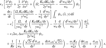 $$\begin{eqnarray}\displaystyle & & \displaystyle \displaystyle \unicode[STIX]{x1D716}_{2}\left[\frac{\unicode[STIX]{x2202}^{2}\unicode[STIX]{x1D713}_{2}}{\unicode[STIX]{x2202}y^{2}}+\frac{1}{2y}\frac{\unicode[STIX]{x2202}^{2}\unicode[STIX]{x1D713}_{2}}{\unicode[STIX]{x2202}x^{2}}+\left(\unicode[STIX]{x1D6FA}_{c}\frac{K_{0}\,\text{d}K_{0}/\text{d}y}{2y^{2}w_{0}^{2}}-\frac{\text{d}^{2}w_{0}/\text{d}y^{2}}{w_{0}}\right)\unicode[STIX]{x1D713}_{2}\right]\nonumber\\ \displaystyle & & \displaystyle \displaystyle \quad =\frac{\text{d}\unicode[STIX]{x1D716}_{1}}{\text{d}t}\left[\frac{\unicode[STIX]{x1D6FA}_{c}K_{0}\,\text{d}K_{0}/\text{d}y}{y^{2}w_{0}^{3}}-\frac{1}{w_{0}^{2}}\frac{\text{d}^{2}w_{0}}{\text{d}y^{2}}\right]\int _{0}^{x}\unicode[STIX]{x1D713}_{1c}(\tilde{x},y)\,\text{d}\tilde{x}\nonumber\\ \displaystyle & & \displaystyle \displaystyle \qquad -\,\unicode[STIX]{x1D716}_{1}^{2}\left[\frac{\unicode[STIX]{x1D6FA}_{c}}{yw_{0}^{3/2}}\frac{\text{d}}{\text{d}y}\left(\frac{K_{0}\,\text{d}K_{0}/\text{d}y}{yw_{0}^{3/2}}\right)-\frac{1}{w_{0}}\frac{\text{d}}{\text{d}y}\left(\frac{\text{d}^{2}w_{0}/\text{d}y^{2}}{w_{0}}\right)\right]\frac{\unicode[STIX]{x1D713}_{1c}^{2}}{2}\nonumber\\ \displaystyle & & \displaystyle \qquad \displaystyle -\,\unicode[STIX]{x1D716}_{1}2\unicode[STIX]{x1D714}_{c}\unicode[STIX]{x0394}\unicode[STIX]{x1D714}\frac{K_{0}\,\text{d}K_{0}/\text{d}y}{2y^{2}w_{0}^{2}}\unicode[STIX]{x1D713}_{1c}\nonumber\\ \displaystyle & & \displaystyle \displaystyle \qquad +\,\frac{1}{Re}\left[\frac{1}{w_{0}}\left(\frac{\sqrt{2y}\,\text{d}^{2}\unicode[STIX]{x1D70E}_{rx0}}{\text{d}y^{2}}+\frac{\text{d}(\unicode[STIX]{x1D70E}_{rx0}/\sqrt{2y})}{\text{d}y}\right)-\frac{\unicode[STIX]{x1D714}_{c}K_{0}}{w_{0}^{2}y}\left(\frac{\text{d}\unicode[STIX]{x1D70E}_{r\unicode[STIX]{x1D703}0}}{\text{d}y}+\frac{\unicode[STIX]{x1D70E}_{r\unicode[STIX]{x1D703}0}}{y}\right)\right]x,\qquad\end{eqnarray}$$
with boundary conditions
 $$\begin{eqnarray}\displaystyle \left.\begin{array}{@{}c@{}}\displaystyle \unicode[STIX]{x1D713}_{2}(x,0)=\unicode[STIX]{x1D713}_{2}(x,1/2)=0\quad \text{for }0\leqslant x\leqslant x_{0},\\ \displaystyle \unicode[STIX]{x1D713}_{2}(0,y)=\frac{\unicode[STIX]{x2202}^{2}\unicode[STIX]{x1D713}_{2}}{\unicode[STIX]{x2202}x^{2}}(0,y)=\unicode[STIX]{x1D713}_{2}(x_{0},y)=0\quad \text{for }0\leqslant y\leqslant 1/2.\end{array}\right\} & & \displaystyle\end{eqnarray}$$
Equation (4.35) is a non-homogeneous partial differential equation for the solution of
 $\unicode[STIX]{x1D716}_{2}(t)\unicode[STIX]{x1D713}_{2}(x,y)$
, subject to homogeneous boundary conditions (4.29) and (4.36). Since the related homogeneous problem has the non-trivial solution
 $\unicode[STIX]{x1D713}_{1c}$
, solvability of (4.35) requires that the forcing term is orthogonal to
 $\unicode[STIX]{x1D713}_{1c}$
. Multiplying (4.35) by
 $\unicode[STIX]{x1D713}_{1c}$
, integrating over the domain (
 $0\leqslant x\leqslant x_{0},0\leqslant y\leqslant 1/2$
) and using the homogeneous boundary conditions for
 $\unicode[STIX]{x1D713}_{2}$
results in the solvability condition,
 $$\begin{eqnarray}\displaystyle & \displaystyle \frac{\text{d}\unicode[STIX]{x1D716}_{1}}{\text{d}t}M_{s}+\unicode[STIX]{x1D716}_{1}^{2}M_{1}-\unicode[STIX]{x1D716}_{1}\unicode[STIX]{x0394}\unicode[STIX]{x1D6FA}M_{2}+\frac{1}{Re}M_{3}=0. & \displaystyle\end{eqnarray}$$
Here,
 $\unicode[STIX]{x0394}\unicode[STIX]{x1D6FA}=2\unicode[STIX]{x1D714}_{c}\unicode[STIX]{x0394}\unicode[STIX]{x1D714}$
and
 $$\begin{eqnarray}\displaystyle & \displaystyle M_{s}=\frac{2x_{0}^{2}}{\unicode[STIX]{x03C0}^{2}}P_{s},\quad M_{1}=\frac{4x_{0}}{3\unicode[STIX]{x03C0}}P_{1},\quad M_{2}=\frac{x_{0}}{2}P_{2},\quad M_{3}=\frac{4x_{0}^{2}}{\unicode[STIX]{x03C0}^{2}}P_{3}, & \displaystyle\end{eqnarray}$$
where
 $$\begin{eqnarray}\displaystyle \left.\begin{array}{@{}c@{}}P_{s}=\displaystyle \int _{0}^{1/2}\left[\frac{\unicode[STIX]{x1D6FA}_{c}K_{0}\,\text{d}K_{0}/\text{d}y}{y^{2}w_{0}^{3}}-\frac{1}{w_{0}^{2}}\frac{\text{d}^{2}w_{0}}{\text{d}y^{2}}\right]\unicode[STIX]{x1D6F7}^{2}(y)\,\text{d}y,\\ P_{1}=\displaystyle -\int _{0}^{1/2}\left[\frac{\unicode[STIX]{x1D6FA}_{c}}{yw_{0}^{3/2}}\frac{\text{d}}{\text{d}y}\left(\frac{K_{0}\,\text{d}K_{0}/\text{d}y}{yw_{0}^{3/2}}\right)-\frac{1}{w_{0}}\frac{\text{d}}{\text{d}y}\left(\frac{\text{d}^{2}w_{0}/\text{d}y^{2}}{w_{0}}\right)\right]\frac{\unicode[STIX]{x1D6F7}^{3}(y)}{2}\,\text{d}y,\\ P_{2}=\displaystyle \int _{0}^{1/2}\frac{K_{0}\,\text{d}K_{0}/\text{d}y}{2y^{2}w_{0}^{2}}\unicode[STIX]{x1D6F7}^{2}(y)\,\text{d}y,\\ P_{3}=\displaystyle \int _{0}^{1/2}\left[\frac{1}{w_{0}}\left(\sqrt{2y}\frac{\text{d}^{2}\unicode[STIX]{x1D70E}_{rx0}}{\text{d}y^{2}}+\frac{\text{d}(\unicode[STIX]{x1D70E}_{rx0}/\sqrt{2y})}{\text{d}y}\right)\right.\\ \quad -\left.\displaystyle \frac{\unicode[STIX]{x1D714}_{c}K_{0}}{w_{0}^{2}y}\left(\frac{\text{d}\unicode[STIX]{x1D70E}_{r\unicode[STIX]{x1D703}0}}{\text{d}y}+\frac{\unicode[STIX]{x1D70E}_{r\unicode[STIX]{x1D703}0}}{y}\right)\right]\unicode[STIX]{x1D6F7}(y)\,\text{d}y.\quad \end{array}\right\} & & \displaystyle\end{eqnarray}$$
It should be noted that to the orders considered here, the stresses according to (3.2)–(3.7) are computed at
 $\unicode[STIX]{x1D714}=\unicode[STIX]{x1D714}_{c}$
, which is a function of the parameters characterizing
 $v_{0}$
and
 $w_{0}$
. Moreover, the parameter
 $P_{3}$
is a function of
 $We$
,
 $\unicode[STIX]{x1D706}$
and
 $a$
. In the case of a Newtonian fluid, where
 $We=0$
, the base flow stresses are given by
 $\unicode[STIX]{x1D70E}_{rx0}=\text{d}w_{0}/\text{d}r$
and
 $\unicode[STIX]{x1D70E}_{r\unicode[STIX]{x1D703}0}=\unicode[STIX]{x1D714}_{c}((\text{d}v_{0}/\text{d}r)-(v_{0}/r))$
. Then, the parameter
 $P_{3}$
as well as all of the following results reduce to those found in Wang & Rusak (Reference Wang and Rusak1997b
). In addition, it can be seen from (3.2)–(3.7) and (4.39) that, for all values of
 $We\neq 0$
, when
 $\unicode[STIX]{x1D706}=1$
(the relaxation and retardation times are equal,
 $\unicode[STIX]{x1D706}_{1}=\unicode[STIX]{x1D706}_{2}$
), both base flow stresses
 $\unicode[STIX]{x1D70E}_{rx0}$
and
 $\unicode[STIX]{x1D70E}_{r\unicode[STIX]{x1D703}0}$
reduce to their expressions for a Newtonian fluid, and to the orders considered, the fluid behaves like a Newtonian fluid.
We note that in the case of high
 $Re$
,
 $We\sim O(1)$
,
 $0<\unicode[STIX]{x1D706}<1$
and
 $0<a<1$
, the model equation (4.37) does not include the normal stresses or the normal stress difference since they contribute effects of higher orders,
 $O(\unicode[STIX]{x1D716}_{1}^{3})$
. Moreover, within the present assumptions, the effects resulting from the unsteady terms in the Giesekus model are also of higher order
 $O(\unicode[STIX]{x1D716}_{1}^{3})$
and are therefore not included in (4.37). When
 $Re$
is high, the dynamics of the flow is determined by lumped inertia effects given by
 $P_{s}$
,
 $P_{1}$
,
 $P_{2}$
and the lumped viscoelastic effect
 $P_{3}$
, similarly to the Newtonian fluid case.
For relevant base rotating flows such as the Rankine vortex, the Lamb–Oseen vortex (
 $\unicode[STIX]{x1D6FF}=0$
) or the Q-vortex (see Leibovich Reference Leibovich1984), it is found that
 $P_{s},P_{1},P_{2}$
and
 $P_{3}$
are usually positive for every vortex core radius,
 $We\sim O(1)$
,
 $\unicode[STIX]{x1D706}$
and
 $a$
.
4.3 The steady-state case
The steady-state version of (4.37) (where
 $\text{d}\unicode[STIX]{x1D716}_{1}/\text{d}t=0$
) has a real solution of
 $\unicode[STIX]{x1D716}_{1}$
if and only if
 $$\begin{eqnarray}\displaystyle & \displaystyle |\unicode[STIX]{x0394}\unicode[STIX]{x1D6FA}|\geqslant \frac{16}{\sqrt{3\unicode[STIX]{x03C0}^{3}}}\frac{\sqrt{P_{1}P_{3}}}{P_{2}}\sqrt{\frac{x_{0}}{Re}}. & \displaystyle\end{eqnarray}$$
When
 $|\unicode[STIX]{x0394}\unicode[STIX]{x1D6FA}|<16/\sqrt{3\unicode[STIX]{x03C0}^{3}}(\sqrt{P_{1}P_{3}}/P_{2})\sqrt{x_{0}/Re}$
, (4.37) has no real solution, indicating that no near-columnar steady solution exists at inlet swirl levels close to the critical state. The states where
 $|\unicode[STIX]{x0394}\unicode[STIX]{x1D6FA}|=16/\sqrt{3\unicode[STIX]{x03C0}^{3}}(\sqrt{P_{1}P_{3}}/P_{2})\sqrt{x_{0}/Re}$
or where
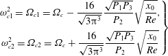 $$\begin{eqnarray}\displaystyle \left.\begin{array}{@{}c@{}}\displaystyle \unicode[STIX]{x1D714}_{c1}^{2}=\unicode[STIX]{x1D6FA}_{c1}=\unicode[STIX]{x1D6FA}_{c}-\frac{16}{\sqrt{3\unicode[STIX]{x03C0}^{3}}}\frac{\sqrt{P_{1}P_{3}}}{P_{2}}\sqrt{\frac{x_{0}}{Re}},\\ \displaystyle \unicode[STIX]{x1D714}_{c2}^{2}=\unicode[STIX]{x1D6FA}_{c2}=\unicode[STIX]{x1D6FA}_{c}+\frac{16}{\sqrt{3\unicode[STIX]{x03C0}^{3}}}\frac{\sqrt{P_{1}P_{3}}}{P_{2}}\sqrt{\frac{x_{0}}{Re}}\end{array}\right\} & & \displaystyle\end{eqnarray}$$
are special states which are saddle fold bifurcation points of solutions of the steady and axisymmetric viscoelastic fluid flow equations of motion. The limit swirl ratios
 $\unicode[STIX]{x1D714}_{c1}$
and
 $\unicode[STIX]{x1D714}_{c2}$
may be considered as the corrections to the inviscid critical swirl as a result of the viscoelastic effects. In the case of a Newtonian fluid, the inlet swirl level
 $\unicode[STIX]{x1D714}_{c1}$
is identified as the first limit point found in the computations of Beran & Culick (Reference Beran and Culick1992).
We also find that near the critical state and when (4.40) is satisfied, there exist two solutions of
 $\unicode[STIX]{x1D716}_{1}$
,
 $$\begin{eqnarray}\displaystyle & \displaystyle \unicode[STIX]{x1D716}_{1}^{\pm }\left(\unicode[STIX]{x0394}\unicode[STIX]{x1D6FA};\frac{1}{Re};We;\unicode[STIX]{x1D706};a\right)=\frac{\unicode[STIX]{x0394}\unicode[STIX]{x1D6FA}P_{2}\pm \sqrt{(\unicode[STIX]{x0394}\unicode[STIX]{x1D6FA})^{2}P_{2}^{2}-256(x_{0}/Re)P_{1}P_{3}/3\unicode[STIX]{x03C0}^{3}}}{16P_{1}/3\unicode[STIX]{x03C0}}.\quad & \displaystyle\end{eqnarray}$$
Here,
 $\unicode[STIX]{x1D716}_{1}^{+}$
corresponds to the
 $+$
sign in front of the square root term in (4.42) and
 $\unicode[STIX]{x1D716}_{1}^{-}$
to the
 $-$
sign in (4.42). Equations (4.1), (4.32) and (4.42) give the asymptotic expansion of the axial velocity
 $w(x,y)$
of the two possible steady states at inlet swirl levels near the critical swirl
 $\unicode[STIX]{x1D714}_{c}$
,
 $$\begin{eqnarray}\displaystyle & \displaystyle w^{\pm }(x,y)=w_{0}(y)+\frac{\unicode[STIX]{x0394}\unicode[STIX]{x1D6FA}P_{2}\pm \sqrt{(\unicode[STIX]{x0394}\unicode[STIX]{x1D6FA})^{2}P_{2}^{2}-256(x_{0}/Re)P_{1}P_{3}/3\unicode[STIX]{x03C0}^{3}}}{16P_{1}/3\unicode[STIX]{x03C0}}~\frac{\text{d}\unicode[STIX]{x1D6F7}(y)}{\text{d}y}\text{sin}\left(\frac{\unicode[STIX]{x03C0}x}{2x_{0}}\right). & \displaystyle \nonumber\\ \displaystyle & & \displaystyle\end{eqnarray}$$
Equation (4.43) illustrates several interesting points. For a high-
 $Re$
flow, the transcritical bifurcation of solutions of the inviscid-limit equations at
 $\unicode[STIX]{x1D714}_{c}$
breaks into two branches of solutions of the viscoelastic fluid flow equations with a finite gap between the two branches, the size of which is
 $\unicode[STIX]{x1D714}_{c2}^{2}-\unicode[STIX]{x1D714}_{c1}^{2}=32/\sqrt{3\unicode[STIX]{x03C0}^{3}}\sqrt{P_{1}P_{3}}/P_{2}\sqrt{x_{0}/Re}$
.
A representative bifurcation diagram of swirling flow behaviour of a viscoelastic fluid in terms of the centreline axial velocity at the pipe outlet,
 $w(x_{0},0)$
, as a function of the inlet swirl ratio,
 $\unicode[STIX]{x1D714}$
, is shown in figure 6. Here, the inlet flow is a Q-vortex (3.9) with an axial jet where
 $\unicode[STIX]{x1D6FD}=4$
,
 $\unicode[STIX]{x1D6FF}=1$
and the pipe length is
 $x_{0}=6$
. The axial velocity at the outlet centreline is calculated from
 $w^{\pm }(x_{0},0)=w_{0}(0)+((\unicode[STIX]{x0394}\unicode[STIX]{x1D6FA}P_{2}\pm \sqrt{(\unicode[STIX]{x0394}\unicode[STIX]{x1D6FA})^{2}P_{2}^{2}-256(x_{0}/Re)P_{1}P_{3}/3\unicode[STIX]{x03C0}^{3}})/(16P_{1}/3\unicode[STIX]{x03C0}))$
. Moreover, in figure 6,
 $Re=1\,000$
,
 $We=1.5$
,
 $\unicode[STIX]{x1D706}=0.5$
and
 $a=0.5$
. For this flow,
 $\unicode[STIX]{x1D714}_{c}=1.5216$
,
 $\unicode[STIX]{x1D714}_{c1}=1.3111$
and
 $\unicode[STIX]{x1D714}_{c2}=1.7320$
. It can be seen that steady near-columnar flow solutions of the viscoelastic fluid flow equations exist for
 $0<\unicode[STIX]{x1D714}<\unicode[STIX]{x1D714}_{c1}$
and
 $\unicode[STIX]{x1D714}>\unicode[STIX]{x1D714}_{c2}$
. For the branch with
 $0<\unicode[STIX]{x1D714}<\unicode[STIX]{x1D714}_{c1}$
, we find that the flow is decelerated along the pipe centreline and the axial velocity reaches a minimum at the pipe outlet. For the branch where
 $\unicode[STIX]{x1D714}>\unicode[STIX]{x1D714}_{c2}$
, the flow is accelerated along the pipe centreline and the axial velocity reaches a maximum at the pipe outlet. The gap between the two branches of solutions disappears and a transcritical bifurcation dominates the flow behaviour in the inviscid-limit flow as
 $Re$
tends to infinity (see figure 6).
The meaning of the gap between the branches of solutions around the critical swirl is that no near-columnar axisymmetric equilibrium state can exist in a finite range of incoming swirl around the critical level,
 $\unicode[STIX]{x1D714}_{c1}<\unicode[STIX]{x1D714}<\unicode[STIX]{x1D714}_{c2}$
. The flow must develop large disturbances in this swirl range. Beyond this gap, when
 $0<\unicode[STIX]{x1D714}<\unicode[STIX]{x1D714}_{c1}$
or
 $\unicode[STIX]{x1D714}>\unicode[STIX]{x1D714}_{c2}$
, there is a range of inlet swirl where two equilibrium states may co-exist under the same inlet/outlet conditions. One, given by the positive root in (4.43), describes a near-columnar flow for which
 $\unicode[STIX]{x1D716}_{1}$
is small in size, and the other, given by the negative root in (4.43), describes a relatively large-amplitude solitary-wave disturbance that either decelerates the axial flow when
 $0<\unicode[STIX]{x1D714}<\unicode[STIX]{x1D714}_{c1}$
or accelerates the flow when
 $\unicode[STIX]{x1D714}>\unicode[STIX]{x1D714}_{c2}$
.
Let
 $\unicode[STIX]{x1D713}(x,y)=\unicode[STIX]{x1D713}_{0}(y)+\unicode[STIX]{x1D716}_{1}\unicode[STIX]{x1D713}_{1}(x,y)$
be the stream function field of the steady-state flow, where
 $\unicode[STIX]{x1D713}_{0}(y)=\int _{0}^{y}w_{0}(y^{\prime })\,\text{d}y^{\prime }$
. Figure 7 presents contours of
 $\unicode[STIX]{x1D713}(x,y)$
for four representative steady states along the branches of the viscoelastic flow solutions shown in figure 6. Figure 7(a) shows the near-columnar state (with a small disturbance) and figure 7(b) describes the large-disturbance state, both found at
 $\unicode[STIX]{x1D714}=1.26$
. In the near-columnar state, the contours are nearly parallel to the centreline, while in the large-disturbance state, the flow is decelerated around the centreline, as reflected by the diverging contours around the centreline. Figures 7(c) and 7(d) show respectively the near-columnar state and the large-disturbance state found at
 $\unicode[STIX]{x1D714}=1.8$
. In the large-disturbance state, the flow is accelerated around the centreline, as reflected by the contracting contours around the centreline.
A representative bifurcation diagram of steady-state solutions of near-critical swirling flows of viscoelastic fluids in a pipe for a Q-vortex (3.9) with
 $\unicode[STIX]{x1D6FD}=4$
,
 $\unicode[STIX]{x1D6FF}=1$
and
 $x_{0}=6$
, where
 $Re=1000$
,
 $We=1.5,$
 $\unicode[STIX]{x1D706}=0.5$
and
 $a=0.5$
. Also shown for reference is the inviscid-limit case, where
 $Re\rightarrow \infty$
.

Contours of
 $\unicode[STIX]{x1D713}(x,y)$
of representative flow states at (a)
 $\unicode[STIX]{x1D714}=1.26$
, the near-columnar state; (b)
 $\unicode[STIX]{x1D714}=1.26$
, the large-disturbance state; (c)
 $\unicode[STIX]{x1D714}=1.8$
, the near-columnar state; (d)
 $\unicode[STIX]{x1D714}=1.8$
, the large-disturbance state. Here,
 $\unicode[STIX]{x1D6FD}=4$
,
 $\unicode[STIX]{x1D6FF}=1$
and
 $x_{0}=6$
. Moreover,
 $Re=1000$
,
 $We=1.5,$
 $\unicode[STIX]{x1D706}=0.5$
and
 $a=0.5$
.

The above results also show that the effect of the non-Newtonian fluid properties on the swirling flow behaviour can be lumped into an effective Reynolds number,
 $$\begin{eqnarray}Re_{eff}=Re~\frac{P_{3\,Newtonian}}{P_{3\,non\text{-}Newtonian}}.\end{eqnarray}$$
Essentially, the effective Reynolds number provides, within the details of the present theory, a simple universal similarity parameter to link between the behaviour of a swirling flow of a non-Newtonian fluid and the respective behaviour of a Newtonian fluid. The use of an effective Reynolds number can be applied to any model for the stresses of a non-Newtonian fluid.
Figure 8 presents three lines: (i)
 $Re_{eff}/Re$
as a function of
 $We$
with fixed values of
 $\unicode[STIX]{x1D706}=0.5$
and
 $a=0.5$
(the solid line); (ii)
 $Re_{eff}/Re$
as a function of
 $\unicode[STIX]{x1D706}$
with fixed values of
 $We=1.5$
and
 $a=0.5$
(the dash–dot line); (iii)
 $Re_{eff}/Re$
as a function of
 $a$
with fixed
 $We=1.5$
and
 $\unicode[STIX]{x1D706}=0.5$
(the dashed line). Here, we use a Q-vortex (3.9) with
 $\unicode[STIX]{x1D6FD}=4$
,
 $\unicode[STIX]{x1D6FF}=1$
and
 $x_{0}=6$
. It is found that
 $Re_{eff}/Re$
always increases above one with increase of
 $We$
and
 $a$
from zero and with decrease of
 $\unicode[STIX]{x1D706}$
from one. The effective Reynolds number is always above the Reynolds number of the flow of a viscoelastic fluid due to the reduction in size of the shear stresses. The most dominant effect is the significant increase of
 $Re_{eff}$
on decreasing
 $\unicode[STIX]{x1D706}$
from one to zero, which is attributed to the increase of corresponding shear-thinning effects. This behaviour causes the increase of the critical swirl
 $\unicode[STIX]{x1D714}_{c1}$
and the decrease of
 $\unicode[STIX]{x1D714}_{c2}$
with the increase of
 $We$
(fluid elasticity) and
 $a$
(mobility) from zero or with the decrease of
 $\unicode[STIX]{x1D706}$
from one (increase of shear thinning).
Plots of
 $Re_{eff}/Re$
as a function of
 $We$
with fixed values
 $\unicode[STIX]{x1D706}=0.5$
and
 $a=0.5$
(the solid line),
 $Re_{eff}/Re$
as a function of
 $\unicode[STIX]{x1D706}$
with fixed
 $We=1.5$
and
 $a=0.5$
(the dash–dot line) and
 $Re_{eff}/Re$
as a function of
 $a$
with fixed
 $We=1.5$
and
 $\unicode[STIX]{x1D706}=0.5$
(the dashed line) for a near-critical swirling flow of viscoelastic fluids in a pipe. Here, we use a Q-vortex (3.9) with
 $\unicode[STIX]{x1D6FD}=4$
,
 $\unicode[STIX]{x1D6FF}=1$
and
 $x_{0}=6$
.

4.4 The stability of steady states
We use the ordinary differential equation (4.37) for the evolution of
 $\unicode[STIX]{x1D716}_{1}(t)$
to study the nonlinear stability of the steady-state solutions determined in § 4.3 in response to an initial perturbation at
 $t=0$
given by
 $\unicode[STIX]{x1D716}_{1}(0)=\unicode[STIX]{x1D716}_{10}$
. When
 $0<\unicode[STIX]{x1D714}<\unicode[STIX]{x1D714}_{c1}$
or
 $\unicode[STIX]{x1D714}>\unicode[STIX]{x1D714}_{c2}$
, the solution of (4.37) gives
 $$\begin{eqnarray}\left|\frac{\unicode[STIX]{x1D716}_{1}(t)-\unicode[STIX]{x1D716}_{1}^{+}}{\unicode[STIX]{x1D716}_{10}-\unicode[STIX]{x1D716}_{1}^{+}}\frac{\unicode[STIX]{x1D716}_{10}-\unicode[STIX]{x1D716}_{1}^{-}}{\unicode[STIX]{x1D716}_{1}(t)-\unicode[STIX]{x1D716}_{1}^{-}}\right|=\exp \left[-\frac{M_{1}}{M_{s}}(\unicode[STIX]{x1D716}_{1}^{+}-\unicode[STIX]{x1D716}_{1}^{-})t\right].\end{eqnarray}$$
It should be noted that
 $\unicode[STIX]{x1D716}_{1}^{+}-\unicode[STIX]{x1D716}_{1}^{-}=\sqrt{(\unicode[STIX]{x0394}\unicode[STIX]{x1D6FA})^{2}P_{2}^{2}-256(x_{0}/Re)P_{1}P_{3}/3\unicode[STIX]{x03C0}^{3}}/(8P_{1}/3\unicode[STIX]{x03C0})>0$
. We find that as
 $t$
tends to infinity,
 $\unicode[STIX]{x1D716}_{1}$
tends to
 $\unicode[STIX]{x1D716}_{1}^{+}$
when
 $\unicode[STIX]{x1D716}_{10}>\unicode[STIX]{x1D716}_{1}^{-}$
. On the other hand, when
 $\unicode[STIX]{x1D716}_{10}<\unicode[STIX]{x1D716}_{1}^{-}$
,
 $\unicode[STIX]{x1D716}_{1}$
evolves to growing negative values within a finite time, indicating the formation of a separation zone around the centreline, on the way to establishing a vortex breakdown state. This means that the steady-state solution with
 $\unicode[STIX]{x1D716}_{1}^{+}$
is nonlinearly asymptotically stable, while the steady-state solution with
 $\unicode[STIX]{x1D716}_{1}^{-}$
is unstable and cannot be realized from the long-term flow dynamics.
Figure 9 demonstrates the evolution of
 $\unicode[STIX]{x1D716}_{1}(t)$
starting from various initial conditions
 $\unicode[STIX]{x1D716}_{10}$
for the case of a Q-vortex (3.9) with
 $\unicode[STIX]{x1D6FD}=4$
,
 $\unicode[STIX]{x1D6FF}=1$
,
 $\unicode[STIX]{x1D714}=1.26$
and
 $x_{0}=6$
, where
 $Re=1000$
,
 $We=1.5,$
 $\unicode[STIX]{x1D706}=0.5$
and
 $a=0.5$
. In this case, the steady-state solutions are
 $\unicode[STIX]{x1D716}_{1}^{+}=-0.5207$
(the dash–dot line) and
 $\unicode[STIX]{x1D716}_{1}^{-}=-2.0440$
(the dashed line). It can be seen that, indeed, starting from all
 $\unicode[STIX]{x1D716}_{10}>\unicode[STIX]{x1D716}_{1}^{-}$
, the solution of
 $\unicode[STIX]{x1D716}_{1}(t)$
approaches
 $\unicode[STIX]{x1D716}_{1}^{+}$
as
 $t$
tends to infinity. However, starting from all
 $\unicode[STIX]{x1D716}_{10}<\unicode[STIX]{x1D716}_{1}^{-}$
, the solution of
 $\unicode[STIX]{x1D716}_{1}(t)$
increases in negative values as
 $t$
increases.
When
 $\unicode[STIX]{x1D714}_{c1}<\unicode[STIX]{x1D714}<\unicode[STIX]{x1D714}_{c2}$
, the solution of (4.37) gives
 $$\begin{eqnarray}\frac{2M_{1}\unicode[STIX]{x1D716}_{1}-\unicode[STIX]{x0394}\unicode[STIX]{x1D6FA}M_{2}}{\sqrt{4M_{1}M_{3}/Re-(\unicode[STIX]{x0394}\unicode[STIX]{x1D6FA})^{2}M_{2}^{2}}}=\tan \left(\frac{1}{2}\sqrt{4M_{1}M_{3}/Re-(\unicode[STIX]{x0394}\unicode[STIX]{x1D6FA})^{2}M_{2}^{2}}\left(-\frac{t}{M_{s}}+C\right)\right).\end{eqnarray}$$
Here,
 $C$
is a constant of integration and is a function of
 $\unicode[STIX]{x1D716}_{10}$
. As
 $t$
approaches a finite value
 $t^{\ast }$
for which the argument of the tangent function on the right-hand side of (4.46) tends to
 $-\unicode[STIX]{x03C0}/2$
,
 $\unicode[STIX]{x1D716}_{1}$
evolves to growing negative values. This indicates again, in the range of swirl
 $\unicode[STIX]{x1D714}_{c1}<\unicode[STIX]{x1D714}<\unicode[STIX]{x1D714}_{c2}$
, the continuous growth of the decelerating flow perturbation along the centreline in a finite time to form a separation zone around the centreline, on the way to establishing a vortex breakdown state. The present small-disturbance theory does not apply anymore after such a situation is established.
Solutions of
 $\unicode[STIX]{x1D716}_{1}$
as a function of time
 $t$
, starting from various initial conditions
 $\unicode[STIX]{x1D716}_{10}$
, for a Q-vortex (3.9) with
 $\unicode[STIX]{x1D6FD}=4$
,
 $\unicode[STIX]{x1D6FF}=1$
,
 $\unicode[STIX]{x1D714}=1.26$
and
 $x_{0}=6$
, where
 $Re=1000$
,
 $We=1.5,$
 $\unicode[STIX]{x1D706}=0.5$
and
 $a=0.5$
. Also shown for reference are the steady-state solutions for this case, a dotted line for
 $\unicode[STIX]{x1D716}_{1}^{+}=-0.5207$
and a dashed line for
 $\unicode[STIX]{x1D716}_{1}^{-}=-2.0440$
.

The stability analysis shows that the branch of the near-columnar flow solutions is asymptotically stable to small axisymmetric disturbances when
 $0<\unicode[STIX]{x1D714}<\unicode[STIX]{x1D714}_{c1}$
and is unstable when
 $\unicode[STIX]{x1D714}>\unicode[STIX]{x1D714}_{c2}$
. Moreover, the branch of large-disturbance solutions that folds backward at
 $\unicode[STIX]{x1D714}_{c1}$
is unstable to axisymmetric disturbances, while the branch of large-disturbance solutions that folds forward at
 $\unicode[STIX]{x1D714}_{c2}$
is asymptotically stable. The limit (fold) points
 $\unicode[STIX]{x1D714}_{c1}$
and
 $\unicode[STIX]{x1D714}_{c2}$
found in the present analysis are also points of exchange of stability of the respective branches of steady-state solutions. This is indicated in figure 6 by the solid lines which represent the stable states and the dashed lines which represent the unstable states. As
 $Re$
tends to infinity, the linear stability results of Wang & Rusak (Reference Wang and Rusak1996, Reference Wang and Rusak1997a
) for the inviscid-limit solutions are recovered. Moreover, the flow simulations of Beran (Reference Beran1994) and Lopez (Reference Lopez1994), based on the unsteady and axisymmetric Navier–Stokes equations, demonstrate the same stability characteristics of near-critical swirling flows for a Newtonian fluid.
5 Computed results
We investigate the effects of
 $We$
,
 $\unicode[STIX]{x1D706}$
and
 $a$
on the nature of near-critical swirling flow states. We demonstrate the present results for the case where the incoming vortex flow is given by the Q-vortex model (3.9).
In the following examples, we first consider an incoming swirling jet flow with the parameters
 $\unicode[STIX]{x1D6FD}=4$
and
 $\unicode[STIX]{x1D6FF}=1$
in a straight circular pipe of length
 $x_{0}=6$
. This base vortex state may represent the rotating flows entering an open vortex tube in the experiments of Leibovich (Reference Leibovich1984). The numerical solution of the eigenvalue problem (4.31) shows that in this case,
 $\unicode[STIX]{x1D714}_{c}=1.5216$
, and from (4.39),
 $P_{1}=0.005498$
and
 $P_{2}=0.015039$
. Moreover, in this case, the base flow stresses
 $\unicode[STIX]{x1D70E}_{rx0}(r)$
and
 $\unicode[STIX]{x1D70E}_{r\unicode[STIX]{x1D703}0}(r)$
for various values of
 $We$
,
 $\unicode[STIX]{x1D706}$
and
 $a$
are shown in figures 3–5. These stress profiles are used to compute the parameter
 $P_{3}$
according to (4.39) for the various values of
 $We$
,
 $\unicode[STIX]{x1D706}$
, and
 $a$
. For example, when the fluid is Newtonian (for
 $We=0$
or for every
 $We$
when
 $\unicode[STIX]{x1D706}=1$
), we find that
 $P_{3}=1.64295$
, whereas when
 $We=1.5$
,
 $\unicode[STIX]{x1D706}=0.5$
and
 $a=0.5$
, we have
 $P_{3}=1.02151$
. A similar behaviour is found with other viscoelastic fluid parameters. We find that for vortex flows with an axial jet profile, the parameter
 $P_{3}$
decreases for the viscoelastic fluid flow. The decrease in size of the stresses
 $\unicode[STIX]{x1D70E}_{r\unicode[STIX]{x1D703}0}$
and
 $\unicode[STIX]{x1D70E}_{rx0}$
(with respect to the Newtonian fluid case) with the increase of either
 $We$
or
 $a$
from
 $0$
, or with the decrease of
 $\unicode[STIX]{x1D706}$
from
 $1$
, increases the effective Reynolds number to
 $Re_{eff}=1.608\,Re$
. This results in a higher value of the first critical inlet swirl level
 $\unicode[STIX]{x1D714}_{c1}$
, and induces transition to breakdown states at higher inlet swirl levels in comparison to the Newtonian fluid behaviour. This viscoelastic fluid behaviour is demonstrated in the following figures.
The bifurcation diagrams of the centreline velocity at the pipe outlet,
 $w(x_{0},0)$
, as a function of the inlet swirl level,
 $\unicode[STIX]{x1D714}$
, for various values of the Weissenberg number,
 $We$
, in the range
 $0$
(a Newtonian fluid) to
 $2$
(with fixed values of
 $\unicode[STIX]{x1D706}=0.5$
and
 $a=0.5$
) are computed and are shown in figure 10(a). In addition, figure 10(b) presents the resulting variation of the critical (fold) swirl level
 $\unicode[STIX]{x1D714}_{c1}$
with changing
 $We$
. We focus here only on the branch of solutions where
 $0\leqslant \unicode[STIX]{x1D714}<\unicode[STIX]{x1D714}_{c}$
. In all cases,
 $Re=1000$
is used and the inviscid-limit flow case with
 $Re\rightarrow \infty$
is again shown for reference. It can be seen that, at the given parameters, the critical swirl ratio
 $\unicode[STIX]{x1D714}_{c1}$
increases as the fluid elasticity (represented by
 $We$
) is increased. The perturbation to the near-columnar states becomes smaller at any fixed level of swirl and the fold behaviour becomes sharper as
 $We$
is increased. It can be concluded that in swirling jet flows, increasing the relaxation time
 $\unicode[STIX]{x1D706}_{1}$
and thereby the fluid elasticity, with the other parameters being fixed, delays the appearance of vortex breakdown to higher inlet swirl levels.
Effect of varying the Weissenberg number from
 $0$
(Newtonian fluid) to
 $2$
on (a) the bifurcation diagrams of steady-state solutions of near-critical swirling flows in a pipe for a Q-vortex (3.9) with
 $\unicode[STIX]{x1D6FD}=4$
,
 $\unicode[STIX]{x1D6FF}=1$
and
 $x_{0}=6$
, where
 $Re=1000$
,
 $\unicode[STIX]{x1D706}=0.5$
and
 $a=0.5$
at various Weissenberg numbers; also shown for reference is the inviscid-limit case where
 $Re\rightarrow \infty$
; (b) the first limit swirl ratio
 $\unicode[STIX]{x1D714}_{c1}$
of near-critical swirling flows in a pipe for a Q-vortex (3.9) with
 $\unicode[STIX]{x1D6FD}=4$
,
 $\unicode[STIX]{x1D6FF}=1$
and
 $x_{0}=6$
, where
 $Re=1000$
,
 $\unicode[STIX]{x1D706}=0.5$
and
 $a=0.5$
.

The effect of changing the characteristic time ratio
 $\unicode[STIX]{x1D706}$
from
 $0$
to
 $1$
(a Newtonian fluid behaviour) on the flow structure is presented in the bifurcation diagrams of
 $w(x_{0},0)$
as a function of
 $\unicode[STIX]{x1D714}$
; see figure 11(a). Here,
 $We=1.5$
,
 $a=0.5$
and
 $Re=1000$
. Moreover, figure 11(b) presents the resulting variation of the critical (fold) swirl ratio
 $\unicode[STIX]{x1D714}_{c1}$
with changing
 $\unicode[STIX]{x1D706}$
. It can be seen that, at the given parameters, the critical swirl ratio
 $\unicode[STIX]{x1D714}_{c1}$
increases from the Newtonian fluid value with the decrease of
 $\unicode[STIX]{x1D706}$
from
 $1$
to
 $0$
. The appearance of vortex breakdown is delayed with the increase of the shear-thinning effects.
The bifurcation diagrams of
 $w(x_{0},0)$
as a function of
 $\unicode[STIX]{x1D714}$
, for various values of the mobility parameter
 $a$
, are computed and shown in figure 12(a). Here,
 $We=1.5$
,
 $\unicode[STIX]{x1D706}=0.5$
and
 $Re=1000$
. Also shown in figure 12(b) is the resulting variation of
 $\unicode[STIX]{x1D714}_{c1}$
with changing
 $a$
. It can be seen that, at the given parameters, the critical swirl ratio
 $\unicode[STIX]{x1D714}_{c1}$
increases as
 $a$
is increased from
 $0$
(an Oldroyd-B fluid) to
 $1$
. Specifically, a significant change of
 $\unicode[STIX]{x1D714}_{c1}$
is found with small changes of
 $a$
from 0 to
 $0.2$
. The perturbation to the near-columnar states becomes smaller at any fixed level of swirl as
 $a$
is increased. Increasing the mobility parameter with the other parameters being fixed also delays the appearance of vortex breakdown to higher inlet swirl levels.
We also study the case of an incoming swirling wake flow with the parameters
 $\unicode[STIX]{x1D6FD}=4$
and
 $\unicode[STIX]{x1D6FF}=-0.3$
in a straight circular pipe of length
 $x_{0}=6.0$
. Bifurcation diagrams of the centreline speed at the outlet
 $w(x_{0},0)$
, as a function of the inlet swirl ratio level
 $\unicode[STIX]{x1D714}$
, for various values of
 $We$
,
 $\unicode[STIX]{x1D706}$
and
 $a$
, are computed (not shown). The resulting changes in the value of the critical swirl level
 $\unicode[STIX]{x1D714}_{c1}$
with variations of
 $We$
,
 $\unicode[STIX]{x1D706}$
and
 $a$
are presented in figure 13(a–c). In all cases,
 $Re=1000$
is considered. It can be seen that
 $\unicode[STIX]{x1D714}_{c1}$
increases with increase of either
 $We$
(fluid elasticity) or
 $a$
from
 $0$
, or with decrease of
 $\unicode[STIX]{x1D706}$
(increase of shear thinning) from
 $1$
. The behaviour of swirling wake flows is similar to that of swirling jet flows, showing the robustness of the viscoelastic effects on the flow critical state.
Effect of varying the characteristic time ratio
 $\unicode[STIX]{x1D706}$
from
 $0$
to
 $1$
(a Newtonian fluid behaviour) on (a) the bifurcation diagrams of steady-state solutions of near-critical swirling flows in a pipe for a Q-vortex (3.9) with
 $\unicode[STIX]{x1D6FD}=4$
,
 $\unicode[STIX]{x1D6FF}=1$
and
 $x_{0}=6$
, where
 $Re=1000$
,
 $We=1.5$
and
 $a=0.5$
; also shown for reference is the inviscid-limit case where
 $Re\rightarrow \infty$
; (b) the first limit swirl ratio
 $\unicode[STIX]{x1D714}_{c1}$
of near-critical swirling flows in a pipe for a Q-vortex (3.9) with
 $\unicode[STIX]{x1D6FD}=4$
,
 $\unicode[STIX]{x1D6FF}=1$
and
 $x_{0}=6$
, where
 $Re=1000$
,
 $We=1.5$
and
 $a=0.5$
.

Effect of varying the mobility parameter
 $a$
on (a) the bifurcation diagrams of steady-state solutions of near-critical swirling flows in a pipe for a Q-vortex (3.9) with
 $\unicode[STIX]{x1D6FD}=4$
,
 $\unicode[STIX]{x1D6FF}=1$
and
 $x_{0}=6$
, where
 $Re=1000$
,
 $We=1.5$
and
 $\unicode[STIX]{x1D706}=0.5$
, at various mobility parameter values from
 $0$
to
 $2$
; also shown for reference is the inviscid-limit case where
 $Re\rightarrow \infty$
; (b) the first limit swirl ratio
 $\unicode[STIX]{x1D714}_{c1}$
of near-critical swirling flows in a pipe for a Q-vortex (3.9) with
 $\unicode[STIX]{x1D6FD}=4$
,
 $\unicode[STIX]{x1D6FF}=1$
and
 $x_{0}=6$
, where
 $Re=1000$
,
 $We=1.5$
and
 $\unicode[STIX]{x1D706}=0.5$
.

(a) Effect of the Weissenberg number on the first limit swirl ratio
 $\unicode[STIX]{x1D714}_{c1}$
of near-critical swirling flows in a pipe for a Q-vortex (3.9) with
 $\unicode[STIX]{x1D6FD}=4$
,
 $\unicode[STIX]{x1D6FF}=-0.3$
and
 $x_{0}=6$
, where
 $Re=1000$
,
 $\unicode[STIX]{x1D706}=0.5$
and
 $a=0.75$
. (b) Effect of the time ratio on the first limit swirl ratio
 $\unicode[STIX]{x1D714}_{c1}$
of near-critical swirling flows in a pipe for a Q-vortex (3.9) with
 $\unicode[STIX]{x1D6FD}=4$
,
 $\unicode[STIX]{x1D6FF}=-0.3$
and
 $x_{0}=6$
, where
 $Re=1000$
,
 $We=2$
and
 $a=0.75$
. (c) Effect of the mobility parameter on the first limit swirl ratio
 $\unicode[STIX]{x1D714}_{c1}$
of near-critical swirling flows in a pipe for a Q-vortex (3.9) with
 $\unicode[STIX]{x1D6FD}=4$
,
 $\unicode[STIX]{x1D6FF}=-0.3$
and
 $x_{0}=6$
, where
 $Re=1000$
,
 $\unicode[STIX]{x1D706}=0.5$
and
 $We=2$
.

6 Discussion
The analysis of near-critical swirling flows of a viscoelastic fluid shows that there exist two limit levels of the inlet swirl ratio,
 $\unicode[STIX]{x1D714}_{c1}$
and
 $\unicode[STIX]{x1D714}_{c2}$
, where equilibrium solutions fold. No near-columnar solution exists in the range of swirl between these two limit swirl ratios, indicating that at these swirl levels the flow must develop large-amplitude disturbances and evolve into vortex breakdown states. Of specific interest is the first limit swirl
 $\unicode[STIX]{x1D714}_{c1}$
, which is the critical swirl for the appearance of vortex breakdown as the inlet swirl ratio is increased. It is found that in Q-vortex flows (3.9) with either an axial jet profile (
 $\unicode[STIX]{x1D6FF}>0$
) or an axial wake profile (
 $\unicode[STIX]{x1D6FF}<0$
), increasing
 $We$
(or the relaxation time) or the mobility parameter
 $a$
, or decreasing the characteristic time ratio
 $\unicode[STIX]{x1D706}$
(or the retardation time) from
 $1$
, causes an increase of
 $\unicode[STIX]{x1D714}_{c1}$
and a delay of vortex breakdown to higher inlet swirl levels. When
 $Re$
is sufficiently high and
 $\unicode[STIX]{x1D714}<\unicode[STIX]{x1D714}_{c1}$
, there is a range of inlet swirl ratios where two equilibrium states may co-exist under the same boundary conditions, one that describes a near-columnar flow and another that describes a large-amplitude solitary wave on the base flow. The size of the disturbances in the flow is affected by changing
 $We$
,
 $\unicode[STIX]{x1D706}$
and
 $a$
.
In addition to these solutions, the theory of Wang & Rusak (Reference Wang and Rusak1997a
) and the numerical flow simulations of Rusak et al. (Reference Rusak, Wang, Xu and Taylor2012, Reference Rusak, Granata and Wang2015) showed the appearance of axisymmetric breakdown states in inviscid and Newtonian fluid vortex flows in a straight circular pipe. These states develop as a branch of linearly stable solutions that is connected to the branch of the unstable large-disturbance solitary-wave states found in the present analysis for
 $Re\rightarrow \infty$
. The branch of vortex breakdown states starts from another limit inlet swirl level
 $\unicode[STIX]{x1D714}_{0}$
(where
 $\unicode[STIX]{x1D714}_{0}<\unicode[STIX]{x1D714}_{c}$
), which is the threshold level of swirl for the appearance of axisymmetric breakdown states (see figure 14). The simulations of Beran (Reference Beran1994), Lopez (Reference Lopez1994) and Rusak et al. (Reference Rusak, Granata and Wang2015) for swirling flows of a Newtonian fluid establish an agreement with the predicted near-columnar states at
 $0<\unicode[STIX]{x1D714}<\unicode[STIX]{x1D714}_{c1}$
, as well as showing the natural evolution to breakdown states when
 $\unicode[STIX]{x1D714}>\unicode[STIX]{x1D714}_{c1}$
. They also demonstrate that
 $\unicode[STIX]{x1D714}_{0\unicode[STIX]{x1D708}}$
for the high-
 $Re$
flow cases is nearly the inviscid-limit value,
 $\unicode[STIX]{x1D714}_{0}$
, when
 $Re>800$
. Moreover, these simulations also show that the breakdown zone is nearly stagnant when
 $Re>800$
.
Expected representative global bifurcation diagrams of axisymmetric steady-state solutions of swirling flows of a Newtonian fluid and a non-Newtonian fluid and their stability characteristics. Here, the inlet flow is a Q-vortex (3.9) with
 $\unicode[STIX]{x1D6FD}=4$
,
 $\unicode[STIX]{x1D6FF}=0$
and
 $x_{0}=6$
. For the non-Newtonian fluid,
 $We=2$
,
 $\unicode[STIX]{x1D706}=0.5$
and
 $a=0.5$
. In both cases,
 $Re=2000$
. Also shown for reference is the bifurcation diagram of the inviscid-limit solutions. The red solid line represents hypothesized breakdown states of non-Newtonian fluid flow.

It is hypothesized that similar vortex breakdown states appear in vortex flows of a viscoelastic fluid and that
 $\unicode[STIX]{x1D714}_{0}$
is nearly independent of
 $Re$
, as well as only slightly affected by the viscoelastic fluid parameters
 $We$
,
 $\unicode[STIX]{x1D706}$
and
 $a$
, specifically when
 $Re$
is sufficiently high (
 $Re>800$
) and
 $We\sim O(1)$
. The various solutions are then summarized in figure 14. The hypothesized viscoelastic flow breakdown solutions are marked by a red solid line. In such cases, it is expected that the viscoelastic flow problem defined by (2.4)–(2.8) with boundary conditions (2.10)–(2.13) has only one near-columnar flow solution when
 $\unicode[STIX]{x1D714}<\unicode[STIX]{x1D714}_{0\unicode[STIX]{x1D708}}$
. Three steady-state solutions may co-exist when
 $\unicode[STIX]{x1D714}$
is in the range of swirl
 $\unicode[STIX]{x1D714}_{0\unicode[STIX]{x1D708}}<\unicode[STIX]{x1D714}<\unicode[STIX]{x1D714}_{c1}$
. One state is a near-columnar asymptotically stable state described by the positive root in (4.43). The second is an unstable large-disturbance solitary-wave state described by the negative root in (4.43). The third state is a stable vortex breakdown state which contains a finite-size near-stagnation zone around the pipe centreline, which may be computed numerically. Only a stable vortex breakdown state exists when
 $\unicode[STIX]{x1D714}_{c1}<\unicode[STIX]{x1D714}<\unicode[STIX]{x1D714}_{c2}$
. When
 $\unicode[STIX]{x1D714}>\unicode[STIX]{x1D714}_{c2}$
, there are again three steady-state solutions, i.e. the nearly columnar state described by the negative root in (4.43) that is unstable, the state with accelerated flow along the pipe centreline described by the positive root in (4.43) that is linearly stable and the vortex breakdown state that is stable. This discussion clarifies the possible steady flow states that may appear in a pipe at various
 $Re>800$
,
 $We\sim O(1)$
,
 $\unicode[STIX]{x1D706}$
,
 $a$
and inlet swirl levels around
 $\unicode[STIX]{x1D714}_{c}$
.
We note that the swirl ratio
 $\unicode[STIX]{x1D714}_{c1}$
is the main critical swirl that dominates the flow dynamics in an open pipe, since the flow transitions to a breakdown state as
 $\unicode[STIX]{x1D714}$
increases above
 $\unicode[STIX]{x1D714}_{c1}$
. Then, with further increase of swirl, the flow cannot move out of the branch of breakdown states even if
 $\unicode[STIX]{x1D714}$
is greater than
 $\unicode[STIX]{x1D714}_{c2}$
. The existence of
 $\unicode[STIX]{x1D714}_{c2}$
does not influence the flow dynamics to breakdown. The simulations of Newtonian fluid flows show (Rusak et al.
Reference Rusak, Granata and Wang2015) that the chances of establishing stable accelerated flow states at
 $\unicode[STIX]{x1D714}>\unicode[STIX]{x1D714}_{c2}$
are very small and require a special set of large-disturbance initial conditions which may not be physically realized in a simple way. Starting with most initial conditions, the flow is attracted to a breakdown state when
 $\unicode[STIX]{x1D714}>\unicode[STIX]{x1D714}_{c1}$
.
In addition, it is found that swirling wake flows of non-Newtonian fluid behave in a similar way to swirling jet flows, thereby demonstrating the robustness of the viscoelastic effects on swirling flows and the resulting delay in the appearance of vortex breakdown. Therefore, it is expected that such effects will appear in other swirling flow situations with vortex breakdown, such as the flows inside a container with a rotating lid.
The trends of the present results show a correlation with the experimental data observed by Stokes et al. (Reference Stokes, Graham, Lawson and Boger2001), where Boger fluids were used. They studied the effect of the viscoelastic properties of fluids on the appearance of vortex breakdown in swirling flows in a closed container with a rotating end wall. They found (see figures 19 and 20 in Stokes et al.
Reference Stokes, Graham, Lawson and Boger2001) that for a fixed high ratio of the container height to radius (greater than 2.5), vortex breakdown appears for the first time at higher swirl levels than those of a Newtonian fluid when the retardation time
 $\unicode[STIX]{x1D706}_{2}$
is decreased from
 $\unicode[STIX]{x1D706}_{1}$
to lower values at a fixed relaxation time
 $\unicode[STIX]{x1D706}_{1}$
. This measured behaviour is reflected in the computed behaviour of
 $\unicode[STIX]{x1D714}_{c1}$
as a function of decreasing
 $\unicode[STIX]{x1D706}$
(shear thinning) from 1 at a fixed
 $We$
, as shown in figure 11(b).
On the other hand, the experimental results in Stokes et al. (Reference Stokes, Graham, Lawson and Boger2001) show that the critical swirl level for vortex breakdown decreases and approaches that of a Newtonian fluid when the relaxation time
 $\unicode[STIX]{x1D706}_{1}$
is increased at a fixed characteristic time ratio. This is in contrast to the computed increase of
 $\unicode[STIX]{x1D714}_{c1}$
as a function of increasing
 $We$
at a fixed
 $\unicode[STIX]{x1D706}$
and
 $a$
, as shown in figure 10(a,b). We may explain the experimental results by also including the effect of the mobility parameter
 $a$
. As demonstrated in appendix A, the experimental viscoelastic fluid with the lower value of
 $\unicode[STIX]{x1D706}_{1}$
(
 $=0.186~\text{ s}$
) (polyacrylamide mixed in
 $75\,\%$
glycerol at various concentrations) has higher values of the mobility parameter
 $a$
than the fluid with the higher value of
 $\unicode[STIX]{x1D706}_{1}$
(
 $=0.838~\text{s}$
) (xanthan gum mixed in
 $75\,\%$
glycerol at various concentrations), which has smaller values of the mobility parameter. According to figure 12(a,b), the critical swirl increases significantly, specifically as
 $a$
increases from
 $0$
to
 $0.2$
. The effect of increasing
 $We$
(or
 $\unicode[STIX]{x1D706}_{1}$
) on
 $\unicode[STIX]{x1D714}_{c1}$
at a fixed
 $\unicode[STIX]{x1D706}=0.8$
for two small values of
 $a$
,
 $0.01$
and
 $0.05$
, is shown in figure 15. It can be seen that the increase of
 $\unicode[STIX]{x1D714}_{c1}$
with
 $We$
is relatively small at
 $a=0.01$
, while it is larger at
 $a=0.05$
. This gives rise to the situation that the critical swirl may actually decrease with increasing
 $We$
(or
 $\unicode[STIX]{x1D706}_{1}$
, fluid elasticity) at a fixed time ratio due to the lower value of the mobility parameter in the viscoelastic fluid with the higher relaxation time; see the two marked points in figure 15, one with a smaller value of
 $We$
and a higher value of
 $\unicode[STIX]{x1D714}_{c1}$
on the line with the higher value of
 $a$
and the second with a four times greater value of
 $We$
and a lower value of
 $\unicode[STIX]{x1D714}_{c1}$
on the line with the near-zero value of
 $a$
. This demonstrates that the combined effects of fluid elasticity and mobility at a fixed
 $\unicode[STIX]{x1D706}$
(shear thinning) can form a situation that is similar to the experimental observations.
The critical swirl
 $\unicode[STIX]{x1D714}_{c1}$
as a function of
 $We$
for
 $a=0.05$
(solid line) and
 $a=0.01$
(dashed line). In both cases, the characteristic time ratio is
 $\unicode[STIX]{x1D706}=0.8$
. The parameters of the Q-vortex (3.9) are
 $\unicode[STIX]{x1D6FD}=4$
and
 $\unicode[STIX]{x1D6FF}=1$
. Also shown by black circles are two representative cases.

7 Conclusions
The interaction between flow inertia and elasticity in high-Reynolds-number, axisymmetric and near-critical swirling flows of an incompressible and viscoelastic fluid in an open finite-length straight circular pipe is studied. The stresses of the viscoelastic fluid are described by the Giesekus constitutive model. This model helps to focus the analysis on the fluid elastic effects as well as shear thinning of the viscosity. The application of the Giesekus model to columnar streamwise vortices is first investigated (§ 3). Then, a nonlinear small-disturbance model problem is developed from the governing equations of motion. It reveals the complicated interactions between flow inertia, swirl and fluid rheology. An effective Reynolds number that links between steady states of swirling flows of a viscoelastic fluid and those of a Newtonian fluid is revealed (4.44). The effects of the fluid viscosity, relaxation time, retardation time and mobility parameter on the flow development in the pipe and on the critical swirl for the appearance of vortex breakdown are explored. It is found that in vortex flows with either an axial jet or axial wake profile, decreasing the ratio of the viscoelastic characteristic times from one to zero (with fixed values of the Weissenberg number and the mobility parameter; i.e., increasing shear thinning) increases the critical swirl ratio for breakdown. Increasing the fluid elasticity through increase of the Weissenberg number from zero (with a fixed ratio of the viscoelastic characteristic times and a fixed value of the mobility parameter) or increasing the fluid mobility parameter from zero (with fixed values of the Weissenberg number and the ratio of viscoelastic times) causes a similar effect. The robustness of the predicted results for the viscoelastic effects on flow dynamics suggests that these effects may appear in other flow apparatuses and can be used to explain the changes in the first appearance of breakdown zones as a function of swirl level that were observed in the experiments by Stokes et al. (Reference Stokes, Graham, Lawson and Boger2001), where Boger fluids were used.
The present work extends, for the first time, the theory of vortex stability and breakdown to include effects of non-Newtonian fluids. It should be noted that the analysis is not limited to the use of the Giesekus model. Equation (4.37) and the definition of
 $Re_{eff}$
(4.44) are general and can be used with any other model that describes the stresses
 $\unicode[STIX]{x1D70E}_{rx0}$
and
 $\unicode[STIX]{x1D70E}_{r\unicode[STIX]{x1D703}0}$
of a viscoelastic flow in terms of the base axial and circumferential velocity fields
 $w_{0}(r)$
and
 $\unicode[STIX]{x1D714}v_{0}(r)$
.
The present study is limited to the behaviour of near-critical swirling flows
 $\unicode[STIX]{x1D714}\sim \unicode[STIX]{x1D714}_{c}$
of high-
 $Re$
laminar viscous fluids with
 $O(1)$
values of
 $We$
(between 0 and 2) and
 $0\leqslant a\leqslant 1$
. The study takes advantage of the assumptions of this special limit case to form a relatively simple nonlinear analytical model problem and explore the fluid flow behaviour. As a result of these model assumptions, the viscoelastic fluid effects are limited in size and result in relatively small variations from the Newtonian swirling flow behaviour. This is exhibited in the results for the critical swirl levels of a flow in an open pipe; see figures 10–13. We note that the experimental investigation of Stokes et al. (Reference Stokes, Graham, Lawson and Boger2001) is also focused on such flow situations with low elasticity, and the robustness of the present model predictions may be used to explain the similar trends of fluid flow behaviour in these experiments, where flows in a closed container with a rotating lid were studied.
It is clear, however, that the present model may not be accurate in prediction of the dynamics of swirling flows of viscoelastic fluids where
 $Re$
is low (less than 300),
 $\unicode[STIX]{x1D714}$
is much greater than
 $\unicode[STIX]{x1D714}_{0}$
, or
 $We$
is high (greater than 10, high fluid elasticity). It is expected that in such flows, more complicated interactions exist between the flow inertia, swirl and viscoelastic effects. These strong viscoelastic and swirl interactions may result in significantly different steady flow states, including the vortex breakdown states, i.e. they may lead to new solutions of flow states non-existent in the Newtonian fluid case, and may further complicate the bifurcation diagram of states. Moreover, they may result in the appearance of a variety of additional instabilities that are driven by the unsteady terms in the constitutive model and do not even exist in Newtonian fluids. The computation of such complex flow situations is probably beyond any simple analytical model and requires extensive numerical simulations of the fluid flow dynamics based on (2.4)–(2.13).
The present paper also focuses on axisymmetric flows. This assumption provides a fundamental case study for flow theoretical analysis that was never performed before. It is also supported by experiments where axisymmetric breakdown states are found (Sarpkaya Reference Sarpkaya1971; Leibovich Reference Leibovich1978; Stokes et al. Reference Stokes, Graham, Lawson and Boger2001). However, experiments on vortex flow stability and breakdown in pipes also show the appearance of three-dimensional disturbances (Sarpkaya Reference Sarpkaya1971; Leibovich Reference Leibovich1984), and these should be studied as well. Such situations are again not amenable to a simple consistent analytical model and require dedicated stability computations and direct numerical simulations which may be addressed in follow-up studies.
Appendix A
In this appendix, we use the generalized Giesekus model to calculate the stresses
 $\bar{\unicode[STIX]{x1D70E}}_{xx}$
,
 $\bar{\unicode[STIX]{x1D70E}}_{xy}$
and
 $\bar{\unicode[STIX]{x1D70E}}_{yy}$
in the case of a two-dimensional parallel shear flow between a stationary wall and a parallel infinite plate at distance
 $h$
moving with a constant velocity
 $U$
in the
 $\bar{x}$
direction. The unidirectional flow velocity components are
 $\bar{v}_{x}=\bar{\dot{\unicode[STIX]{x1D6FE}}}\bar{y}$
,
 $\bar{v}_{y}=\bar{v}_{z}=0$
, where
 $\bar{\dot{\unicode[STIX]{x1D6FE}}}=U/h$
. For this base flow, the model equations (2.2) give
 $$\begin{eqnarray}\displaystyle & \displaystyle \bar{\unicode[STIX]{x1D70E}}_{xx}+a\frac{\unicode[STIX]{x1D706}_{1}}{\unicode[STIX]{x1D702}_{0}}({\bar{\unicode[STIX]{x1D70E}}_{xx}}^{2}+{\bar{\unicode[STIX]{x1D70E}}_{xy}}^{2})-2a\unicode[STIX]{x1D706}_{2}\bar{\dot{\unicode[STIX]{x1D6FE}}}\bar{\unicode[STIX]{x1D70E}}_{xy}-2\unicode[STIX]{x1D706}_{1}\bar{\dot{\unicode[STIX]{x1D6FE}}}\bar{\unicode[STIX]{x1D70E}}_{xy}+a\frac{{\unicode[STIX]{x1D706}_{2}}^{2}}{\unicode[STIX]{x1D706}_{1}}\unicode[STIX]{x1D702}_{0}\bar{\dot{\unicode[STIX]{x1D6FE}}}^{2}+2\unicode[STIX]{x1D706}_{2}\unicode[STIX]{x1D702}_{0}\bar{\dot{\unicode[STIX]{x1D6FE}}}^{2}=0, & \displaystyle\end{eqnarray}$$
 $$\begin{eqnarray}\displaystyle & \displaystyle \bar{\unicode[STIX]{x1D70E}}_{xy}+a\frac{\unicode[STIX]{x1D706}_{1}}{\unicode[STIX]{x1D702}_{0}}(\bar{\unicode[STIX]{x1D70E}}_{xx}\bar{\unicode[STIX]{x1D70E}}_{xy}+\bar{\unicode[STIX]{x1D70E}}_{xy}\bar{\unicode[STIX]{x1D70E}}_{yy})-a\unicode[STIX]{x1D706}_{2}\bar{\dot{\unicode[STIX]{x1D6FE}}}(\bar{\unicode[STIX]{x1D70E}}_{xx}+\bar{\unicode[STIX]{x1D70E}}_{yy})-\unicode[STIX]{x1D706}_{1}\bar{\dot{\unicode[STIX]{x1D6FE}}}\bar{\unicode[STIX]{x1D70E}}_{yy}-\unicode[STIX]{x1D702}_{0}\bar{\dot{\unicode[STIX]{x1D6FE}}}=0, & \displaystyle\end{eqnarray}$$
 $$\begin{eqnarray}\displaystyle & \displaystyle \bar{\unicode[STIX]{x1D70E}}_{yy}+a\frac{\unicode[STIX]{x1D706}_{1}}{\unicode[STIX]{x1D702}_{0}}({\bar{\unicode[STIX]{x1D70E}}_{xy}}^{2}+{\bar{\unicode[STIX]{x1D70E}}_{yy}}^{2})-2a\unicode[STIX]{x1D706}_{2}\bar{\dot{\unicode[STIX]{x1D6FE}}}\bar{\unicode[STIX]{x1D70E}}_{xy}+a\frac{{\unicode[STIX]{x1D706}_{2}}^{2}}{\unicode[STIX]{x1D706}_{1}}\unicode[STIX]{x1D702}_{0}\bar{\dot{\unicode[STIX]{x1D6FE}}}^{2}=0. & \displaystyle\end{eqnarray}$$
We demonstrate in figure 16 that with proper values of
 $\unicode[STIX]{x1D702}_{0}$
,
 $\unicode[STIX]{x1D706}_{1}$
,
 $\unicode[STIX]{x1D706}_{2}$
and
 $a$
, the Giesekus model provides a relevant representation of the nature of the viscosity
 $\unicode[STIX]{x1D702}=\unicode[STIX]{x1D70E}_{xy}/\bar{\dot{\unicode[STIX]{x1D6FE}}}$
(in Pa s) as a function of the shear rate
 $\bar{\dot{\unicode[STIX]{x1D6FE}}}$
(in
 $\text{s}^{-1}$
) found in the experimental rheological measurements of various Boger fluids shown in figure 12 of Stokes et al. (Reference Stokes, Graham, Lawson and Boger2001). The symbols represent the experimental data points and the lines are the curve-fit lines. Also shown for reference in each panel is the constant viscosity of the Newtonian solvent. Figure 16(a) presents the viscosity
 $\unicode[STIX]{x1D702}$
(in Pa s) as a function of the shear rate
 $\bar{\dot{\unicode[STIX]{x1D6FE}}}$
(in
 $\text{s}^{-1}$
) for various concentrations of polyacrylamide (PPA) mixed in
 $75\,\%$
glycerol. The relaxation time is
 $\unicode[STIX]{x1D706}_{1}=0.186$
s for all concentrations. The mixture with 25 p.p.m. of PPA is characterized by
 $\unicode[STIX]{x1D702}_{0}=0.042~\text{Pa}~\text{s}$
,
 $\unicode[STIX]{x1D706}_{2}/\unicode[STIX]{x1D706}_{1}=0.94$
and
 $a=0.01$
. The mixture with 45 p.p.m. of PPA is characterized by
 $\unicode[STIX]{x1D702}_{0}=0.045~\text{Pa}~\text{s}$
,
 $\unicode[STIX]{x1D706}_{2}/\unicode[STIX]{x1D706}_{1}=0.88$
and
 $a=0.03$
. The mixture with 75 p.p.m. of PPA is characterized by
 $\unicode[STIX]{x1D702}_{0}=0.050~\text{Pa}~\text{s}$
,
 $\unicode[STIX]{x1D706}_{2}/\unicode[STIX]{x1D706}_{1}=0.79$
and
 $a=0.05$
. Similarly, figure 16(b) presents the viscosity
 $\unicode[STIX]{x1D702}$
(in Pa s) as a function of the shear rate
 $\bar{\dot{\unicode[STIX]{x1D6FE}}}$
(in
 $\text{s}^{-1}$
) for various concentrations of xanthan gum (XG) mixed in
 $75\,\%$
glycerol. For all concentrations,
 $\unicode[STIX]{x1D706}_{1}=0.838~\text{s}$
. The mixture with 25 p.p.m. of XG is characterized by
 $\unicode[STIX]{x1D702}_{0}=0.051~\text{Pa}~\text{s}$
,
 $\unicode[STIX]{x1D706}_{2}/\unicode[STIX]{x1D706}_{1}=0.77$
and
 $a=0.02$
. The mixture with 45 p.p.m. of XG is characterized by
 $\unicode[STIX]{x1D702}_{0}=0.063~\text{Pa}~\text{s}$
,
 $\unicode[STIX]{x1D706}_{2}/\unicode[STIX]{x1D706}_{1}=0.63$
and
 $a=0.1$
. The mixture with 75 p.p.m. of XG is characterized by
 $\unicode[STIX]{x1D702}_{0}=0.095~\text{Pa}~\text{s}$
,
 $\unicode[STIX]{x1D706}_{2}/\unicode[STIX]{x1D706}_{1}=0.42$
and
 $a=0.25$
. An increase in either PPA or XG concentration results in a decrease of
 $\unicode[STIX]{x1D706}_{2}$
and an increase of
 $a$
with a fixed
 $\unicode[STIX]{x1D706}_{1}$
. The use of XG results in higher values of
 $\unicode[STIX]{x1D706}_{1}$
and
 $a$
. It should be noted, however, that the mixture with 75 p.p.m. of PPA and the mixture with 25 p.p.m. of XG have nearly the same ratio of
 $\unicode[STIX]{x1D706}_{2}/\unicode[STIX]{x1D706}_{1}\sim 0.78$
, but the first fluid has a higher value of the mobility parameter
 $a$
than the second fluid.
The viscosity
 $\unicode[STIX]{x1D702}$
(in Pa s) as a function of the shear rate (in
 $\text{s}^{-1}$
) for various Boger fluids. The symbols are from experimental data in figure 12 in Stokes et al. (Reference Stokes, Graham, Lawson and Boger2001) and the lines are curve-fit representations according to the Giesekus model. (a) Polyacrylamide mixed in 75 % glycerol at various concentrations, 25 p.p.m. (short dashed line and circles), 45 p.p.m. (intermediate dashed line and squares) and 75 p.p.m. (long dashed line and diamonds). Also shown for reference is the solid line for the solvent. (b) Xanthan gum mixed in 75 % glycerol at various concentrations, 25 p.p.m. (short dashed line and circles), 45 p.p.m. (intermediate dashed line and squares) and 75 p.p.m. (long dashed line and diamonds). Also shown for reference is the solid line for the Newtonian solvent.