1. Introduction
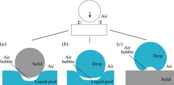
The impact of a drop or a solid sphere onto a liquid pool can encompass various types of air entrainment. One possibility is that air is entrained at the top of the impacting object when the crater that is created during impact collapses, see for example Oguz & Prosperetti (Reference Oguz and Prosperetti1990), Pumphrey & Elmore (Reference Pumphrey and Elmore1990), Wang, Kuan & Tsai (Reference Wang, Kuan and Tsai2013) and Chen & Guo (Reference Chen and Guo2014). Another type of air entrainment may occur at the bottom of the impacting object: the thin air film that is squeezed out at the impact zone is accompanied by a pressure increase that deforms the interface of the liquid before the impacting object touches the pool, which may result in air entrapment (Thoroddsen, Etoh & Takehara Reference Thoroddsen, Etoh and Takehara2003; Thoroddsen et al. Reference Thoroddsen, Etoh, Takehara, Ootsuka and Hatsuki2005; Marston, Vakarelski & Thoroddsen Reference Marston, Vakarelski and Thoroddsen2011; Hicks et al. Reference Hicks, Ermanyuk, Gavrilov and Purvis2012; Tran et al. Reference Tran, De Maleprade, Sun and Lohse2013). The early stages of deformations can be described analytically (Bouwhuis et al. Reference Bouwhuis, Hendrix, Van Der Meer and Snoeijer2015). In the case where the impacting object is a drop, instead of a single entrapped bubble, a collection of microscopic bubbles may also be entrapped, which can create intriguing morphologies (Thoroddsen et al. Reference Thoroddsen, Thoraval, Takehara and Etoh2012). This is also referred to as Mesler entrainment (Esmailizadeh & Mesler Reference Esmailizadeh and Mesler1986; Pumphrey & Elmore Reference Pumphrey and Elmore1990). The same mechanism that is responsible for bubble entrapment at the bottom of an impacting object on a pool holds for air entrapment at the bottom of an impacting drop onto a solid (van Dam & Le Clerc Reference van Dam and Le Clerc2004; Hicks & Purvis Reference Hicks and Purvis2010; Mani, Mandre & Brenner Reference Mani, Mandre and Brenner2010; Bouwhuis et al. Reference Bouwhuis, Van Der Veen, Tran, Keij, Winkels, Peters, Van Der Meer, Sun, Snoeijer and Lohse2012). In fact, the initial geometries of the problems are identical; see figure 1 in which the different impact scenarios and air entrapment have been depicted. We also refer to figure 5 of Tran et al. (Reference Tran, De Maleprade, Sun and Lohse2013), who first worked out this analogy.
Air bubble entrapment for different impact scenarios. Bubbles and deformations are not drawn to scale. (a) Rigid sphere impact onto a pool. The pool deforms due to an increase in air pressure right under the sphere before it touches the pool, which results in an entrapped air bubble. (b) Drop impact onto a pool. Not only the pool, but also the drop, consists of a deformable interface. As a result, the increased air pressure deforms both the pool and the drop and an air bubble is entrapped. (c) Drop impact onto a solid. Here also, a local increase in air pressure deforms the drop before it touches the solid and results in an entrapped air bubble.

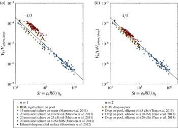
Previously, air bubble entrapment for drop impact onto a solid surface has been quantified experimentally, theoretically and numerically (Mandre, Mani & Brenner Reference Mandre, Mani and Brenner2009; Hicks & Purvis Reference Hicks and Purvis2010, Reference Hicks and Purvis2011; Mani et al. Reference Mani, Mandre and Brenner2010; Bouwhuis et al. Reference Bouwhuis, Van Der Veen, Tran, Keij, Winkels, Peters, Van Der Meer, Sun, Snoeijer and Lohse2012). If the effect of surface tension can be neglected, we can consider the inertial regime (Bouwhuis et al. Reference Bouwhuis, Van Der Veen, Tran, Keij, Winkels, Peters, Van Der Meer, Sun, Snoeijer and Lohse2012), for which the following scaling for the entrapped air bubble volume was found:
 $$\begin{eqnarray}V_{b}/V_{drop}\sim St^{-4/3}.\end{eqnarray}$$
Here,
 $V_{b}/V_{drop}$
is the air bubble volume normalized by the drop volume and
 $\mathit{St}$
is the Stokes number, which is defined as
 $St\equiv {\it\rho}_{l}RU/{\it\eta}_{g}$
, where
 ${\it\rho}_{l}$
is the liquid density,
 $R$
is the droplet radius,
 $U$
is its impact velocity and
 ${\it\eta}_{g}$
is the viscosity of the surrounding gas, in this case air. The Stokes number represents the competing effects of the viscous force of the draining air film and the inertial force of the liquid, which ultimately determine the air bubble volume. The same scaling was found experimentally for impact of a sphere onto a pool (Marston et al.
Reference Marston, Vakarelski and Thoroddsen2011) and a drop onto a pool (Tran et al.
Reference Tran, De Maleprade, Sun and Lohse2013). When surface tension effects become important, the scaling must be modified to include the effect of the Laplace pressure as we move towards the capillary regime (Bouwhuis et al.
Reference Bouwhuis, Van Der Veen, Tran, Keij, Winkels, Peters, Van Der Meer, Sun, Snoeijer and Lohse2012). In recent work, the connection between the capillary and inertial regimes has been captured in a unifying theory (Klaseboer, Manica & Chan Reference Klaseboer, Manica and Chan2014).
In this paper, we try to capture the mechanism of air entrapment during impact onto a deep pool numerically. We will employ a boundary integral method (BIM) for potential flow describing the liquid phase coupled to viscous lubrication theory for the draining microscopic air film. The advantage of using a BIM becomes evident when the interface of the impacting object comes close to the pool and one has to resolve the microscopic air layer together with the macroscopic liquid scale. This difference in length scales can be a thousandfold for the case of a millimetre-sized drop impacting onto a pool squeezing out an air film with a typical thickness of micrometres. In fact, the difference in length scales in the final stages of impact diverges to infinity as the drop is about to coalesce with the pool. Using a BIM guarantees excellent interface representation, since all variables such as liquid velocity and pressure are defined at the interface. At the same time, the computational cost is modest, since the BIM allows the potential problem to be solved only at the boundaries of the liquid domain: quantities in interior points can be calculated optionally as a function of the solution at the boundary. To achieve the same accurate interface representation and solve the full Navier–Stokes equations, using for example a volume-of-fluid method (see for example Thoraval et al. (Reference Thoraval, Takehara, Etoh, Popinet, Ray, Josserand, Zaleski and Thoroddsen2012), Guo et al. (Reference Guo, Wei, Liang and Shen2014)), one would require a much larger computational cost.
In § 2, we explain the theoretical framework together with the numerical method. In § 3, we will present the results of numerical simulation: we will identify details of the pressure development in the air film and deformation of the interfaces at the impact zone. The results of the numerical model will be compared with available results regarding the entrapped bubble volume from multiple experimental works and will be compared with the scaling law equation (1.1). We conclude with § 4 in which suggestions for further research are discussed.
2. Theory
2.1. Dimensional analysis and numerical method
Since the deformation of the interfaces responsible for air entrapment exhibits axial symmetry, we make use of an axisymmetric framework throughout the paper. The Reynolds number of the liquid drops we model, which is defined as
 $Re_{l}\equiv {\it\rho}_{l}RU/{\it\eta}_{l}$
, is assumed to be large,
 $Re_{l}\gg 1$
. Here,
 ${\it\rho}_{l}$
and
 ${\it\eta}_{l}$
are respectively the density and the dynamic viscosity of the liquid,
 $U$
is the impact velocity and
 $R$
is the radius of the drop. The flow can thus be regarded as irrotational, that is
 $\boldsymbol{{\rm\nabla}}\times \boldsymbol{u}=\mathbf{0}$
. Under the additional constraint of incompressible flow inside the drop this allows the liquid dynamics to be modelled with a harmonic function
 ${\it\phi}$
, to which the velocity field
 $\boldsymbol{u}$
is related through
 $$\begin{eqnarray}\boldsymbol{u}=\boldsymbol{{\rm\nabla}}{\it\phi}.\end{eqnarray}$$
The fact that the velocity potential
 ${\it\phi}$
obeys the Laplace equation
 $\boldsymbol{{\rm\nabla}}^{2}{\it\phi}=0$
is used to efficiently solve the potential problem, and thus the dynamics of the liquid, using the BIM. We use a BIM based on codes that are described in detail in Oguz & Prosperetti (Reference Oguz and Prosperetti1993) and Gekle & Gordillo (Reference Gekle and Gordillo2011). While the Reynolds number of the drop is large, the Reynolds number of the thin gaseous air layer,
 $Re_{g}\equiv {\it\rho}_{g}H_{d}U/{\it\eta}_{g}$
, is typically small. Here,
 ${\it\rho}_{g}$
is the gas density and
 $H_{d}$
is the air film thickness in the centre of the film which is referred to as the dimple height. When inserting typical parameters,
 ${\it\rho}_{g}$
is of order
 $1$
,
 $H_{d}$
is of order
 $10^{-6}$
,
 $U$
is of order
 $1$
and
 ${\it\eta}_{g}$
is of order
 $10^{-5}$
. This results in
 $Re_{g}$
being of the order of
 $10^{-1}$
, which justifies the assumption. The length scale characterizing the air layer in the lateral extension of the air film is denoted by
 $L$
, see figure 2(a). As shown in Bouwhuis et al. (Reference Bouwhuis, Van Der Veen, Tran, Keij, Winkels, Peters, Van Der Meer, Sun, Snoeijer and Lohse2012),
 $H_{d}\ll L$
, which in combination with the low Reynolds number of the gas allows the film to be described with viscous lubrication theory, see for example Leal (Reference Leal1992). For droplets impacting with a higher speed well outside the parameter range currently considered, lubrication theory should be extended to include the effect of inertia of the gas. The dimensionless group reflecting the presence of air is the Stokes number
 $\mathit{St}\equiv {\it\rho}_{l}RU/{\it\eta}_{g}$
, which compares the viscous force of the air layer with the inertial force in the drop. This number is relevant for describing dimple formation, since, for high enough impact velocity
 $U$
, this process is determined by two competing forces: the force of the viscous air layer trying to deform the drop in the centre and the opposing inertial force of the drop, which must be slowed down locally in order to form a dimple. Additional dimensionless numbers incorporating the surface tension
 ${\it\gamma}$
are the Weber number
 $\mathit{We}$
and the capillary number
 $\mathit{Ca}$
based on the gas properties. Summarizing, we thus have the following dimensionless parameters:
 $$\begin{eqnarray}Re_{l}\equiv \frac{{\it\rho}_{l}RU}{{\it\eta}_{l}},\quad Re_{g}\equiv \frac{{\it\rho}_{g}H_{d}U}{{\it\eta}_{g}},\quad St\equiv \frac{{\it\rho}_{l}RU}{{\it\eta}_{g}},\quad We\equiv \frac{{\it\rho}_{l}RU^{2}}{{\it\gamma}},\quad Ca\equiv \frac{We}{St}.\end{eqnarray}$$
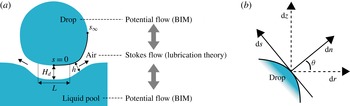
(a) Schematic of drop impact onto a pool. The methods used are indicated in the figure: both the liquid domains are modelled with potential flow, while the air layer is described with Stokes flow. The grey arrows indicate that the flow of the air film is coupled to the dynamics of the liquid domains, and vice versa. (b) Definition of the (
 $n,s$
)-coordinate system, where
 $s$
is aligned along the drop curve and
 $n$
is the unit normal with respect to the drop.

The impact of a liquid drop onto a pool of the same liquid and the impact of a rigid sphere onto a liquid pool can be described with the same dimensionless numbers. As the initial geometries of the problems are identical, the difference lies in the deformability of the object, which is zero in the case of the solid. The two effective control parameters that we will use here in our theoretical framework are
 $\mathit{St}$
and
 $\mathit{We}$
. In this work, the depth of the pool is considered to be infinite. In the case where the thickness of the pool is finite, the dynamics of the pool may be altered due to the presence of a solid boundary at the bottom of the pool. For the impact onto a liquid film with finite thickness we refer the reader to Korobkin, Ellis & Smith (Reference Korobkin, Ellis and Smith2008), in which the impact onto a wetted solid is discussed.
In figure 2(a), an illustration of the impact of a drop onto a pool, together with the method used, is shown. As is clear from this figure, the coupling between the dynamics of the air layer and the dynamics of the liquid is essential since the two liquid domains feel each other through the pressure build-up in the viscous air layer. The lubrication pressure
 $P_{g}$
acts on the liquid surface and appears in the unsteady Bernoulli equation which serves as a dynamic boundary condition in the BIM applied at the liquid surface, see also Bouwhuis et al. (Reference Bouwhuis, Van Der Veen, Tran, Keij, Winkels, Peters, Van Der Meer, Sun, Snoeijer and Lohse2012):
 $$\begin{eqnarray}\left(\frac{\partial {\it\phi}}{\partial t}+\frac{1}{2}\left|\boldsymbol{{\rm\nabla}}{\it\phi}\right|^{2}\right)=-\frac{{\it\gamma}}{{\it\rho}_{l}}{\it\kappa}(s,t)-\frac{P_{g}(s,t)}{{\it\rho}_{l}}.\end{eqnarray}$$
Here,
 $P_{g}$
is the pressure in excess of the ambient pressure, due to lubrication. The curvature of the interface is represented by
 ${\it\kappa}(s,t)$
, which is a function of the curvilinear coordinate
 $s$
, which follows the liquid surface and time
 $t$
. It should be noted that unlike Bouwhuis et al. (Reference Bouwhuis, Van Der Veen, Tran, Keij, Winkels, Peters, Van Der Meer, Sun, Snoeijer and Lohse2012) we do not include gravitation, to make sure that the impact speed of the impacting droplet stays constant. The small deformation of the pool justifies the assumption of neglecting the pressure due to hydrostatic gradients. As we have two liquid domains, two separate boundary integral equations are solved. We take the width of the pool large enough to approach the dynamics of an infinite liquid pool. In this case, a width of 4.5 times the drop radius is found to be sufficient. We focus on quantifying the amount of entrapped air by integrating the enclosed air pocket up to the moment the air layer reaches a physical minimum thickness of
 $0.4~{\rm\mu}\text{m}$
. At this point the volume of the enclosed air has converged and a subsequent rupture of the air film will prevent further drainage, which results in an entrapped air bubble (Bouwhuis et al.
Reference Bouwhuis, Van Der Veen, Tran, Keij, Winkels, Peters, Van Der Meer, Sun, Snoeijer and Lohse2012). As we focus on the dynamics just prior to rupture we can make use of an axisymmetric framework. In Hicks et al. (Reference Hicks, Ermanyuk, Gavrilov and Purvis2012), a similar approach was used to predict the radius of the entrapped bubble that occurs when a solid sphere approaches a liquid free surface. We restrict ourselves to the inertial regime (Bouwhuis et al.
Reference Bouwhuis, Van Der Veen, Tran, Keij, Winkels, Peters, Van Der Meer, Sun, Snoeijer and Lohse2012) for which experimental results (Tran et al.
Reference Tran, De Maleprade, Sun and Lohse2013) are available for a direct comparison. Since the air layer continually deforms and translates during the impact, lubrication equations have been developed in a moving coordinate system that is aligned with the interface of the drop. These equations will be derived in the next section.
2.2. Lubrication in a moving and tilted coordinate system
In this section we develop an expression for the pressure
 $P_{g}$
in the air film based on lubrication theory in a moving (
 $n$
,
 $s$
)-coordinate system that is aligned along the drop surface; see the sketch in figure 2. The reason for doing this (rather than just using the standard (
 $r,z$
)-coordinate system) is that especially for the drop onto pool impact, the moving (
 $n,s$
)-coordinate system is not necessarily oriented like the (
 $r,z$
)-coordinate system and therefore only the first guarantees an accurate description of the draining air film. In appendix A a case is described that shows the difference between lubrication calculated in the two coordinate systems. The drop surface is taken as a reference, and the curvilinear coordinate
 $s$
is defined along the drop, starting at the axis of symmetry. At some large radial coordinate
 $s_{\infty }$
we assume atmospheric pressure. The coordinate perpendicular to
 $s$
is defined to be
 $n$
. The gap thickness
 $h(r,t)$
is defined as the length of the perpendicular line from the drop projected onto the liquid pool. The two surfaces in the impact zone are assumed to be nearly parallel (
 $\left|\partial _{s}h\right|\ll 1$
), so we can apply lubrication theory.
It can be shown (see appendix B) that the continuity equation in this new (
 $n$
,
 $s$
)-coordinate system reads
 $$\begin{eqnarray}\frac{u_{r}}{r}+\partial _{s}u_{s}+\partial _{n}u_{n}=0.\end{eqnarray}$$
At the interface of the liquid pool (
 $n=h$
) we know that the fluid particles have to move with the interface. This is mathematically described with the kinematic boundary condition
 $$\begin{eqnarray}\partial _{t}h+(u_{s}\partial _{s}h)|_{n=h}=u_{n\mid n=h}-u_{n\mid n=0}.\end{eqnarray}$$
Here,
 $\partial _{t}h$
is the time derivative of
 $h$
. We now integrate (2.4) along the gap thickness
 $h$
and obtain
 $$\begin{eqnarray}\int _{0}^{h}\frac{u_{r}}{r}\,\text{d}n+\int _{0}^{h}\partial _{s}u_{s}\,\text{d}n=-\int _{0}^{h}\partial _{n}u_{n}\,\text{d}n=u_{n\mid n=0}-u_{n\mid n=h}.\end{eqnarray}$$
Using the Leibniz integral rule for the second integral on the left-hand side we find
 $$\begin{eqnarray}\int _{0}^{h}\frac{u_{r}}{r}\,\text{d}n+\partial _{s}\int _{0}^{h}u_{s}\,\text{d}n-\left(u_{s}\left.\partial _{s}h\right)\right|_{n=h}=u_{n\mid n=0}-u_{n\mid n=h}.\end{eqnarray}$$
We now use the kinematic boundary condition formulated in (2.5) for the third term on the left-hand side to obtain
 $$\begin{eqnarray}\int _{0}^{h}\frac{u_{r}}{r}\,\text{d}n+\partial _{s}\int _{0}^{h}u_{s}\,\text{d}n+\partial _{t}h-u_{n\mid n=h}+u_{n\mid n=0}=u_{n\mid n=0}-u_{n\mid n=h}.\end{eqnarray}$$
Cancelling the terms
 $u_{n\mid n=h}$
and
 $u_{n\mid n=0}$
on both sides gives
 $$\begin{eqnarray}\int _{0}^{h}\frac{u_{r}}{r}\,\text{d}n+\partial _{s}\int _{0}^{h}u_{s}\,\text{d}n+\partial _{t}h=0.\end{eqnarray}$$
We still have to describe
 $u_{r}$
within the new (
 $s$
,
 $n$
)-coordinate system. Therefore, we substitute
 $u_{r}=u_{n}\cos {\it\theta}-u_{s}\sin {\it\theta}$
in the equation above to obtain
 $$\begin{eqnarray}\int _{0}^{h}\frac{1}{r}u_{n}\cos {\it\theta}\,\text{d}n-\int _{0}^{h}\frac{1}{r}u_{s}\sin {\it\theta}\,\text{d}n+\partial _{s}\int _{0}^{h}u_{s}\,\text{d}n+\partial _{t}h=0.\end{eqnarray}$$
We assume that the main flow of the air that is squeezed out from the gap is along the
 $s$
coordinate, which implies that
 $u_{n}$
is relatively small, so we neglect the first term. The second term is an integral with respect to
 $n$
containing the variable
 $r$
. This radial coordinate
 $r$
across
 $h$
is a function of
 $n$
:
 $r=n\cos {\it\theta}+c(s)$
. Here,
 $c(s)$
is the value of
 $r$
at the drop surface (
 $n=0$
) for some coordinate
 $s$
. We thus substitute this expression for
 $r$
into (2.10) and neglect the first term to find
 $$\begin{eqnarray}-\int _{0}^{h}\frac{\sin {\it\theta}}{n\cos {\it\theta}+c(s)}u_{s}\,\text{d}n+\partial _{s}\int _{0}^{h}u_{s}\,\text{d}n+\partial _{t}h=0.\end{eqnarray}$$
2.2.1. Flow profile within the air film
As has been previously described, the Reynolds number of the thin air film is small,
 $Re_{g}\ll 1$
, and the geometry of the problem,
 $H_{d}\ll L$
, allows us to use lubrication theory. In the (
 $n,s$
)-coordinate system, the Stokes equations can then be reduced to
 $$\begin{eqnarray}\partial _{s}P_{g}={\it\eta}_{g}\partial _{n}^{2}u_{s}.\end{eqnarray}$$
We can integrate (2.12) twice with respect to
 $n$
, employing a no-slip boundary condition at the drop surface (
 $u_{s}=U_{d}$
at
 $n=0$
) as well as at the surface of the pool (
 $u_{s}=U_{p}$
at
 $n=h$
):
 $$\begin{eqnarray}u_{s}=\left((U_{p}-U_{d})\frac{n}{h}+U_{d}\right)+\frac{1}{2{\it\eta}_{g}}\partial _{s}P_{g}(n^{2}-nh).\end{eqnarray}$$
The first term of (2.13) can be associated with Couette flow, caused by the movement of the interfaces. The terms
 $U_{p}$
and
 $U_{d}$
can be extracted by differentiating the potential
 ${\it\phi}$
with respect to the tangential direction of the liquid surface. The second term can be associated with Poiseuille flow, which is driven by the pressure gradient, see also Klaseboer et al. (Reference Klaseboer, Chevaillier, Gourdon and Masbernat2000). Substituting this expression for
 $u_{s}$
in our equation for mass conservation, (2.11), we obtain
 $$\begin{eqnarray}\displaystyle & & \displaystyle -\int _{0}^{h}\frac{\sin {\it\theta}}{n\cos {\it\theta}+c}\left[\left((U_{p}-U_{d})\frac{n}{h}+U_{d}\right)+\frac{1}{2{\it\eta}_{g}}\partial _{s}(n^{2}-nh)\right]\text{d}n\nonumber\\ \displaystyle & & \displaystyle \quad +\,\partial _{s}\int _{0}^{h}\left[\left((U_{p}-U_{d})\frac{n}{h}+U_{d}\right)+\frac{1}{2{\it\eta}_{g}}\partial _{s}P_{g}(n^{2}-nh)\right]\text{d}n+\partial _{t}h=0.\end{eqnarray}$$
In the first integral we deal with a prefactor
 $\sin {\it\theta}/(n\cos {\it\theta}+c)$
. When taking the geometry of the problem into account we note that
 $n\cos {\it\theta}\ll c$
. We can thus write
 $\sin {\it\theta}/(n\cos {\it\theta}+c)\approx \sin {\it\theta}/c$
. Performing the integrals of (2.14) under this assumption yields
 $$\begin{eqnarray}\displaystyle -\frac{\sin {\it\theta}}{c}\left(\frac{h}{2}\left(U_{p}+U_{d}\right)-\frac{h^{3}}{12{\it\eta}_{g}}\partial _{s}P_{g}\right)+\partial _{s}\left(\frac{h}{2}\left(U_{p}+U_{d}\right)-\frac{h^{3}}{12{\it\eta}_{g}}\partial _{s}P_{g}\right)+\partial _{t}h=0.\qquad & & \displaystyle\end{eqnarray}$$
If we define
 $G(s)\equiv (h/2(U_{p}+U_{d})-(h^{3}/12{\it\eta}_{g})\partial _{s}P_{g})$
we can transform the above equation into a first-order inhomogeneous linear ordinary differential equation (ODE) for
 $G(s)$
:
 $$\begin{eqnarray}{\dot{G}}(s)-a(s)G(s)=f(s).\end{eqnarray}$$
Here,
 $a(s)$
and
 $f(s)$
are known functions of
 $s$
:
 $$\begin{eqnarray}a(s)=\frac{\sin {\it\theta}}{c(s)},\end{eqnarray}$$
 $$\begin{eqnarray}f(s)=-\partial _{t}h.\end{eqnarray}$$
2.2.2. Solving the first-order inhomogeneous ODE for
 $G(s)$

Equation (2.16) can be solved with the help of an integrating factor
 $I$
, defined as
 $I(s)\equiv \text{e}^{-\int a(s)\,\text{d}s}$
. Using the boundary condition
 $G(s)=0$
for
 $s=0$
, because we have zero pressure gradient in the centre of symmetry, and also zero tangential velocities, we can multiply (2.16) with
 $I(s)$
and solve for
 $G(s)$
:
 $$\begin{eqnarray}G(s)=\frac{1}{I(s)}\left(\int _{0}^{s}I(\tilde{s})f(\tilde{s})\,\text{d}\tilde{s}\right),\end{eqnarray}$$
with
 $I(s)=\text{e}^{-\int _{0}^{s}a(\tilde{s})\,\text{d}\tilde{s}}$
.
We can now substitute
 $G(s)\equiv (h/2(U_{p}+U_{d})-(h^{3}/12{\it\eta}_{g})\partial _{s}P_{g})$
back into (2.19) to obtain an equation for
 $\partial _{s}P_{g}$
:
 $$\begin{eqnarray}\partial _{s}P_{g}=-\frac{12{\it\eta}_{g}}{h^{3}}\left(\frac{1}{I(s)}\left(\int _{0}^{s}I(\tilde{s})f(\tilde{s})\,\text{d}\tilde{s}\right)-\frac{h}{2}\left(U_{p}+U_{d}\right)\right).\end{eqnarray}$$
We note that we have to evaluate two numerical integrals to calculate
 $\partial _{s}P_{g}$
. In order to find the pressure
 $P_{g}(s)$
, we integrate (2.20) using atmospheric pressure for some large value for
 $s_{\infty }$
well outside the thin air gap as a boundary value. As a check of our analysis we now orientate the (
 $n$
,
 $s$
)-coordinate system in such a way that
 $s=r$
, to recover the lubrication equation in the conventional (
 $r,z$
)-coordinate system. In that case, we have
 ${\it\theta}=-{\rm\pi}/2$
, and we can write for
 $a(s)$
 $$\begin{eqnarray}a(s=r)=\frac{\sin {\it\theta}}{r}=-\frac{1}{r}.\end{eqnarray}$$
The integrating factor
 $I$
now becomes
 $$\begin{eqnarray}I(s=r)=\text{e}^{-\int _{0}^{r}a(\tilde{r})\,\text{d}\tilde{r}}=\text{e}^{\ln r}=r.\end{eqnarray}$$
Substituting (2.22) into (2.20), using the proposition
 $s=r$
and setting
 $U_{b}=0$
and
 $U_{d}=0$
, we can now write (2.20) as
 $$\begin{eqnarray}\partial _{r}P_{g}=-\frac{12{\it\eta}_{g}}{h^{3}}\left(\frac{1}{I(r)}\left(\int _{0}^{r}I(\tilde{r})f(\tilde{r})\,\text{d}\tilde{r}\right)-\frac{h}{2}\left(U_{b}+U_{d}\right)\right)=\frac{12{\it\eta}_{g}}{h^{3}}\left(\frac{1}{r}\left(\int _{0}^{r}\tilde{r}\partial _{t}h\,\text{d}\tilde{r}\right)\right).\end{eqnarray}$$
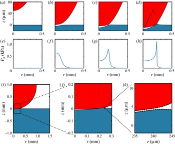
(a–h) Drop impact onto a liquid pool: (a,e)
 $t=0$
, (b,f)
 $t=0.13$
, (c,g)
 $t=0.15$
, (d,h)
 $t=0.17$
. Note the different length scales for the
 $r$
-axis and
 $z$
-axis in the shape plots. The impact speed is
 $U=0.42~\text{m}~\text{s}^{-1}$
and the drop radius is
 $R=0.95~\text{mm}$
. The density and surface tension of the liquid are respectively
 ${\it\rho}=916~\text{kg}~\text{m}^{-3}$
and
 ${\it\gamma}=0.020~\text{N}~\text{m}^{-1}$
. These impact parameters correspond to
 $\mathit{St}=2.0\times 10^{4}$
and
 $\mathit{We}=7.7$
. The simulation starts at time
 $t=0\;\text{ms}$
at a separation of
 $h_{r=0}=50~{\rm\mu}\text{m}$
. Due to the approach of the drop, the excess air pressure
 $P_{g}$
will increase and acts on both the drop and the liquid pool (
 $t=0.13\;\text{ms}$
). At the final stage (
 $t=0.17\;\text{ms}$
) the minimum separation of the interfaces reaches
 $0.4~{\rm\mu}\text{m}$
and the simulation is stopped. The bubble volume
 $V_{b}$
can thus be determined. (i–k) Part of the simulation domain with detailed snapshots of the air film at
 $t=0.17\;\text{ms}$
. In (k), the actual node distribution around the smallest separation point can be inspected. This is the most refined distribution of computational nodes that is used. For the region outside the gap a coarser node distribution is sufficient.

We check by inspection that this (2.23) is the equation for the radial pressure gradient for viscous lubrication theory in the conventional (
 $r,z$
)-coordinate system (Bouwhuis et al.
Reference Bouwhuis, Winkels, Peters, Brunet, Van Der Meer and Snoeijer2013), which gives a consistency check for our analysis. This was also numerically verified.
3. Results
In this section, simulation results will be discussed, starting with § 3.1 in which the drop impact onto a pool will be treated. The interface deformations and pressure development in the viscous air layer will be quantified. In § 3.2, we will focus on rigid sphere impact onto a pool. For both impact scenarios we will quantify the size of the air bubble that is entrapped and directly compare with various experimental results (Marston et al. Reference Marston, Vakarelski and Thoroddsen2011; Bouwhuis et al. Reference Bouwhuis, Van Der Veen, Tran, Keij, Winkels, Peters, Van Der Meer, Sun, Snoeijer and Lohse2012; Tran et al. Reference Tran, De Maleprade, Sun and Lohse2013). In § 3.3, we will compare the dynamics of both impact scenarios and identify symmetrical behaviour.
3.1. Drop impact onto a pool
Figure 3(a–h) displays a typical result for drop impact onto a pool. The results are expressed in dimensional form to match the experimental conditions of the work of Tran et al. (Reference Tran, De Maleprade, Sun and Lohse2013), with which the numerical results in this work will be compared. In figure 3(a) corresponding to
 $t=0\;\text{ms}$
, the initial condition of the simulation at the impact zone is shown. An initial separation of
 $h_{0}=50~{\rm\mu}\text{m}$
is used. Convergence tests regarding the initial release height have been conducted, and an initial separation of
 $h_{0}=50~{\rm\mu}\text{m}$
was found to be appropriate for the lubrication pressure to be still negligible at this distance for the parameter range that is of interest in this study. At
 $t=0.13\;\text{ms}$
(figure 3
b) it can be seen that the pool and the drop experience the increased air pressure and thus the interfaces deform. In figure 3(f), the increase in pressure is indeed visible. At
 $t=0.15\;\text{ms}$
(figure 3
c) the drop is getting closer to the pool, and the interfaces have been further deformed. It can also be noted that the pressure maximum corresponds to the location where the separation between the drop and the pool is smallest. The location of smallest separation is now not located in the centre at
 $r=0$
anymore. This behaviour is typical for impact events involving a free surface and has been experimentally observed for, e.g., drop impact onto a pool (Thoroddsen et al.
Reference Thoroddsen, Thoraval, Takehara and Etoh2012; Tran et al.
Reference Tran, De Maleprade, Sun and Lohse2013), drop impact onto a solid surface (van der Veen et al.
Reference van der Veen, Tran, Lohse and Sun2012), sphere impact onto a pool (Marston et al.
Reference Marston, Vakarelski and Thoroddsen2011) and bubble impact onto a wall in a liquid tank (Hendrix et al.
Reference Hendrix, Manica, Klaseboer, Chan and Ohl2012). In figure 3(d) at
 $t=0.17\;\text{ms}$
, we observe that the two interfaces are very close together, having a minimum separation of
 $0.4~{\rm\mu}\text{m}$
.
We note that the interfaces up to the final stage of impact are very well resolved, see figure 3(i–k) in which figure 3(d) at
 $t=0.17\;\text{ms}$
is shown on various scales while keeping the same length scale for both axes. In figure 3(i), a macroscopic view of the simulation domain is shown. In figure 3(j), the impact zone is selected and magnified. The slender geometry of the microscopic air film can be noted. In figure 3(k), the region of closest separation is magnified. Indeed, the interfaces are very close together, the minimum separation is
 $0.4~{\rm\mu}\text{m}$
. The computational nodes used for discretization of the surface are also shown in this final figure. An adaptive grid on the fluid surface allows for local refinement at the region of closest separation, which results in the total number of nodes being only of order 100, while capturing both the microscopic dynamics at the impact zone and the large-scale motion of the millimetre-sized drop. It should be noted that the slanted orientation of the free surfaces in figure 3(i–k) justifies the need to use a description in terms of the (
 $s$
,
 $n$
)- rather than the (
 $r,z$
)-coordinate system.
We further note from figure 3(d) that a microscopic air film finds itself trapped between the drop and the pool. It is this entrapped air that constitutes the air bubble that is dragged into the liquid when the air film ruptures at the thinnest point and breaks the axisymmetry of the problem. In this work, we do not attempt to simulate the complex rupture process of the air film itself, which is ultimately determined by surface chemistry, see for example Saylor & Bounds (Reference Saylor and Bounds2012). Instead, we focus on the dynamics up to the rupture point, which is taken to happen at a rupture thickness of
 $0.4~{\rm\mu}\text{m}$
. At this point, the volume of the entrained air has converged and can thus be determined, see figure 3(d). This procedure is in line with previous research (Bouwhuis et al.
Reference Bouwhuis, Van Der Veen, Tran, Keij, Winkels, Peters, Van Der Meer, Sun, Snoeijer and Lohse2012), where experimentally the volume of the air pocket just before rupture was indeed found to be identical to the volume of the entrapped bubble. In Thoroddsen et al. (Reference Thoroddsen, Thoraval, Takehara and Etoh2012), the final thickness of the air film is estimated to be of the order of
 ${\sim}0.2~{\rm\mu}\text{m}$
. The final thickness that is reached during an experiment depends on the type of fluid and is sensitive to experimental conditions, e.g. how clean the fluid is (Saylor & Bounds Reference Saylor and Bounds2012). Here, we choose to stick to a minimum thickness consistent with Bouwhuis et al. (Reference Bouwhuis, Van Der Veen, Tran, Keij, Winkels, Peters, Van Der Meer, Sun, Snoeijer and Lohse2012), which is
 $0.4~{\rm\mu}\text{m}$
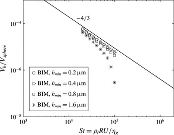
. In appendix C, a figure is included which shows that the volume of the air bubble that can be identified numerically has indeed converged for a minimum thickness of
 $0.4~{\rm\mu}\text{m}$
by also including the bubble volumes calculated for a minimum thickness of
 $0.2~{\rm\mu}\text{m}$
.
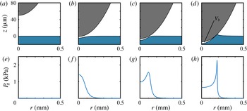
Rigid sphere impact onto a pool: (a,e)
 $t=0$
, (b,f)
 $t=0.12$
, (c,g)
 $t=0.13$
, (d,h)
 $t=0.15$
ms. The impact speed is
 $U=0.42~\text{m}~\text{s}^{-1}$
and the radius is
 $R=0.95~\text{mm}$
. The density and surface tension of the fluid are respectively
 ${\it\rho}=916~\text{kg}~\text{m}^{-3}$
and
 ${\it\gamma}=0.020~\text{N}~\text{m}^{-1}$
. These impact parameters correspond to
 $\mathit{St}=2.0\times 10^{4}$
and
 $\mathit{We}=7.7$
.

3.2. Rigid sphere impact onto a pool
The impact of a sphere onto a pool prior to coalescence is similar to the case of a drop impacting on a pool, except that in the case of an impacting sphere the deformability of the impacting object is zero. This scenario has been simulated by letting an undeformable sphere approach the pool. The same equations are solved as described in § 2, except that no BIM is needed for the impacting sphere since the interface of the sphere is fixed. The result is depicted in figure 4. Just as in the case of drop impact onto a pool, a microscopic air bubble is entrapped, see figure 4(d). As can be seen by inspection, the air bubble has a similar shape, but its size is smaller than in the case of drop impact onto the pool, as can be inferred from a comparison with figure 3(d).
The size of the air bubble can be quantified from the numerical simulation and is compared for both drop impact and sphere impact onto a pool with various experimental results in figure 5(a). We see that the numerical results for both drop and sphere impact onto a pool are in quantitative agreement with experimental work. We note that the numerical results show that the air bubble volume is indeed larger when a drop instead of a sphere impacts onto a pool for all values of
 $\mathit{St}$
, which is supported by the experiments of Tran et al. (Reference Tran, De Maleprade, Sun and Lohse2013). Furthermore, we observe that the numerical results are in agreement with the scaling law presented in (1.1),
 $V_{b}/V_{drop}\sim St^{-4/3}$
. As experiments have shown, in this regime, the viscosity of the liquid is not important for the final bubble volume that is entrapped, see Marston et al. (Reference Marston, Vakarelski and Thoroddsen2011) and Tran et al. (Reference Tran, De Maleprade, Sun and Lohse2013), which is again confirmed by the current modelling technique which captures the essential physics that determines the air bubble volume: a potential flow calculation that does not involve liquid viscosity coupled to viscous lubrication theory for the intervening air layer.
Figure adapted from Tran et al. (Reference Tran, De Maleprade, Sun and Lohse2013). Boundary integral method results are superimposed as yellow symbols. (a) Various experimental data for the normalized bubble volume
 $V_{b}/V_{sphere/drop}$
are shown. Excellent quantitative agreement was found with numerical results. (b) The data, both numerical and experimental, were found to collapse onto one single curve by normalizing
 $V_{b}$
as
 $V_{b}/(nV_{sphere/drop})$
, with
 $n$
the number of free interfaces involved during impact. This number is 2 instead of 1 in the case of drop impact onto a liquid pool.

3.3. Deformations of interfaces: symmetrical behaviour
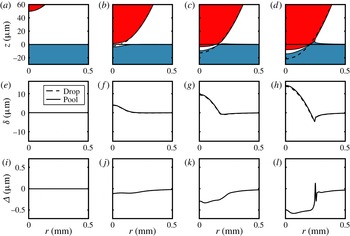
We will now further investigate the fact that the bubble volume for drop impact onto a pool is larger compared with the case where we deal with only one deformable interface during impact, as is the case with rigid sphere impact onto a pool. In figure 6, a closer inspection of the drop impact onto a pool is depicted. In this figure, we track the relative deformation of both the pool and the drop, denoted by
 ${\it\delta}_{drop}$
and
 ${\it\delta}_{pool}$
respectively. Here,
 ${\it\delta}_{drop}$
is defined as the deformation of the drop relative to an undeformed sphere impacting with constant speed
 $U$
, and
 ${\it\delta}_{pool}$
is defined as the deformation of the pool relative to the horizon
 $z=0$
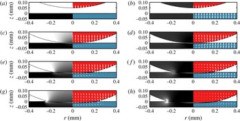
. Interestingly, we note that both interface deformations behave identically. One may expect that two deformable interfaces that react similarly to an external pressure will deform in an identical way. It should be noted, however, that the upper domain (drop) and the lower domain (pool) do not have the same unperturbed geometry, due to the radius of curvature of the drop. Since both media respond identically to the pressure pulse, the weak curvature with respect to the width of the localized pressure has a negligible influence: on the scale of the pressure pulse, both domains are essentially flat. We therefore expect to recover a symmetric response in the upper and lower domains. To illustrate this further, we compute the kinetic energy and the velocity inside the drop and the pool using a technique described in Sun et al. (Reference Sun, Klaseboer, Khoo and Chan2014) to evaluate quantities close to the interface which need special attention as the singular behaviour of the Green’s function in the boundary integral equation becomes apparent for these points. Figure 7(a,c,e,g) shows the result in the frame of the pool. To highlight the symmetry, we also evaluate these quantities in a frame moving at a speed
 $U/2$
in an upward direction, which results in a frame of reference in which both the drop and the pool move with a speed
 $U/2$
towards each other. Indeed, the velocity fields and kinetic energies are now identically distributed, see figure 7(b,d,f,h).
This implies that there will be a larger entrapped air bubble compared with the case where only one of the interfaces is able to deform. To quantify this hypothesis we compare the bubble sizes of drop and sphere impact onto a pool and find a factor 2 difference, see figure 5(b). Here, half of the air bubble volume of drop impact onto a pool was found to collapse onto the experimental and numerical results incorporating only one deformable interface, i.e. sphere impact onto a pool but also drop impact onto a solid. Tran et al. (Reference Tran, De Maleprade, Sun and Lohse2013) took another approach to collapse the data of bubble volumes of drop impact onto a pool by correcting the corresponding impact
 $\mathit{St}$
number by a factor 2, which also collapses the data. In the present work, it is shown that an approach based on considering the number of deformable interfaces (either 1 or 2) can also serve to obtain a unifying view on the air bubble entrapment.
Drop impact onto a pool with a corresponding plot of the relative deformation
 ${\it\delta}$
of both the pool and the drop; (d) shows the definition of
 ${\it\delta}$
: (a,e,i)
 $t=0$
, (b,f,j)
 $t=0.13$
, (c,g,k)
 $t=0.15$
, (d,h,l)
 $t=0.17$
ms. We observe excellent overlap between the relative deformations, which is emphasized in (i–l) where
 ${\it\Delta}={\it\delta}_{drop}-{\it\delta}_{pool}$
, the difference between the two relative deformations, is shown. The same impact conditions as for the case described in figure 3 are used: the impact speed is
 $U=0.42~\text{m}~\text{s}^{-1}$
and the radius is
 $R=0.95~\text{mm}$
. The density and surface tension of the liquid are respectively
 ${\it\rho}=916~\text{kg}~\text{m}^{-3}$
and
 ${\it\gamma}=0.020~\text{N}~\text{m}^{-1}$
, which correspond to
 $\mathit{St}=2.0\times 10^{4}$
and
 $\mathit{We}=7.7$
.

Kinetic energy monitoring during drop impact onto a pool, with impact parameters as described in figure 3, for times (a,b)
 $t=0$
, (c,d)
 $t=0.13$
, (e,f)
 $t=0.15$
, (g,h)
 $t=0.17~\text{ms}$
. (a,c,e,g) In the left half, the kinetic energy
 $K$
is grey-scale coded: black is zero kinetic energy; white is maximum kinetic energy in the system, which is
 $K={\it\rho}U^{2}/2$
. (b,d,f,h) The kinetic energy is recalculated in a moving reference frame moving upwards at
 $U/2$
. This results in a frame of reference in which both the pool and the drop move with a speed of
 $U/2$
towards each other. Again, the left half shows the kinetic energy. We observe a symmetric behaviour, which supports the hypothesis that the pool and the drop react in a symmetric way to the local pressure increase.

4. Conclusion
In this work, air entrapment during liquid drop and rigid sphere impact onto a deep liquid pool has been numerically investigated using a BIM for potential flow for the liquid phase coupled to the viscous lubrication approximation for the subphase air that is squeezed out during impact. Excellent agreement with experimental work was found when comparing the amount of air that is entrained during impact. When considering drop impact onto a pool, both liquid interfaces were found to deform identically relative to their undeformed shape. This leads to an explanation as to why bubble volumes in the case of drop impact onto a pool were found to be twice the size of those that are found, both experimentally and numerically, in impact events involving only one deformable interface, that is rigid sphere impact onto a pool and drop impact onto a solid. In this study, compressibility effects of the air have been neglected. It can be expected that at higher impact velocity compressibility of the intervening air will be important, see for example Hicks & Purvis (Reference Hicks and Purvis2011). In addition, the current modelling technique is limited to an axisymmetric 2D framework. To account for 3D impact problems, for which experimental data are starting to emerge (van der Veen et al. Reference van der Veen, Hendrix, Tran, Sun, Tsai and Lohse2014), the modelling technique needs to be extended to 3D. With a 3D model oblique collisions can also be investigated.
Acknowledgement
We gratefully acknowledge J. Marston and T. Tran for providing their original experimental data set. We would also like to acknowledge R. Hagmeijer for useful suggestions. This work was supported by STW and NWO through a VIDI grant no. 11304.
Drop impact onto a liquid pool: (a,e)
 $t=0.30$
, (b,f)
 $t=0.50$
, (c,g)
 $t=1.50$
, (d,h)
 $t=3.00$
ms. The impact speed is
 $U=0.14~\text{m}~\text{s}^{-1}$
and the drop radius is
 $R=0.95~\text{mm}$
. The density and surface tension of the liquid are respectively
 ${\it\rho}=916~\text{kg}~\text{m}^{-3}$
and
 ${\it\gamma}=0.020~\text{N}~\text{m}^{-1}$
. These impact parameters correspond to
 $\mathit{St}=6.7\times 10^{3}$
and
 $\mathit{We}=0.85$
. (a–d) The macroscopic droplet shape together with the pool shape is shown. The solid line corresponds to calculations made in the moving (
 $n,s$
)-coordinate system. The dashed line shows the result for the same case with the only difference being that lubrication is now calculated in a conventional (
 $r,z$
)-coordinate system. (e–h) To illustrate the different behaviour of the two approaches, the corresponding film thicknesses are shown. It can be seen that in the final stage of impact, the draining of the film behaves differently.

Appendix A. Comparison of the conventional
$(r,z)$
-coordinate system with the moving
$(n,s)$
-coordinate system


The advantage of the moving (
 $n$
,
 $s$
)-coordinate system to calculate the lubrication pressure becomes evident when the interfaces start to deform and the thin air film is not aligned with the (
 $r,z$
)-coordinate system anymore. To illustrate this, we selected a case of drop impact onto a pool as shown and described in figure 8. In figure 8(a–d), we can see by inspection that the two different lubrication methods yield similar results from a macroscopic point of view. However, when focusing on the film thickness
 $h$
between the two interfaces, shown in figure 8(e–h), the difference between the two methods becomes apparent. We note that in the first stages of impact (up to
 $t=0.50~\text{ms}$
), the air film is still aligned with the (
 $r,z$
)-coordinate system, and the two lubrication methods yield similar results. However, in the final stages of impact, the drop sinks deeper into the pool and the air film is not aligned anymore with the (
 $r,z$
)-coordinate system. The (
 $r,z$
)-coordinate system therefore is now no longer adequate, which is reflected in the thinning behaviour which starts to differ from the results obtained with the (
 $n$
,
 $s$
)-coordinate system that moves with the drop. In the final stage (
 $t=3.00~\text{ms}$
), the conventional (
 $r,z$
)-coordinate system clearly shows a wrong film profile, as the minimum gap thickness is now located at the centre
 $r=0$
, while it should be located off-centre, as shown by many experiments (Hicks et al.
Reference Hicks, Ermanyuk, Gavrilov and Purvis2012; Thoroddsen et al.
Reference Thoroddsen, Thoraval, Takehara and Etoh2012; van der Veen et al.
Reference van der Veen, Tran, Lohse and Sun2012; Tran et al.
Reference Tran, De Maleprade, Sun and Lohse2013). This underpins the need for an appropriate moving (
 $n$
,
 $s$
)-coordinate system, from which the conventional (
 $r,z$
)-coordinate system is a special case that is recovered when the lubrication gap is aligned with the (
 $r,z$
)-axes. While upfront it may not be clear whether the interfaces deform to such an extent that a moving coordinate system is needed, it will take into account possible deformations and guarantees accurate lubrication calculations in any scenario.
Appendix B. Continuity in curvilinear coordinates
To derive (2.4) in an (
 $n,s$
)-coordinate system that moves along with the drop surface, see figure 2, we start from the continuity equation in axisymmetric (
 $r,z$
) coordinates:
 $$\begin{eqnarray}\frac{u_{r}}{r}+\frac{\partial u_{r}}{\partial r}+\frac{\partial u_{z}}{\partial z}=0.\end{eqnarray}$$
We now want to write the last two terms of the left-hand side of (B 1) in terms of the (
 $n,s$
)-coordinate system, that is
 $$\begin{eqnarray}\frac{u_{r}}{r}+\frac{\partial u_{r}}{\partial r}+\frac{\partial u_{z}}{\partial z}=\frac{u_{r}}{r}+\left(\frac{\partial u_{r}}{\partial n}\frac{\partial n}{\partial r}+\frac{\partial u_{r}}{\partial s}\frac{\partial s}{\partial r}\right)+\left(\frac{\partial u_{z}}{\partial n}\frac{\partial n}{\partial z}+\frac{\partial u_{z}}{\partial s}\frac{\partial s}{\partial z}\right).\end{eqnarray}$$
The two coordinate systems are related as follows (see also figure 2):
 $$\begin{eqnarray}\displaystyle \text{d}s=-\text{d}r\sin {\it\theta}+\text{d}z\cos {\it\theta}, & & \displaystyle\end{eqnarray}$$
 $$\begin{eqnarray}\displaystyle \text{d}n=\text{d}r\cos {\it\theta}+\text{d}z\sin {\it\theta}. & & \displaystyle\end{eqnarray}$$
Using the relation above we can write (B 2) as
 $$\begin{eqnarray}\frac{u_{r}}{r}+\frac{\partial u_{r}}{\partial r}+\frac{\partial u_{z}}{\partial z}=\frac{u_{r}}{r}+\left(\frac{\partial u_{r}}{\partial n}\cos {\it\theta}-\frac{\partial u_{r}}{\partial s}\sin {\it\theta}\right)+\left(\frac{\partial u_{z}}{\partial n}\sin {\it\theta}+\frac{\partial u_{z}}{\partial s}\cos {\it\theta}\right).\end{eqnarray}$$
Sphere impact onto a pool, with impact parameters as described in figure 4. The bubble volume calculated for different rupture thicknesses
 $h_{min}$
is shown. At a rupture thickness
 $h_{min}$
of
 $0.4~{\rm\mu}\text{m}$
the air bubble volume is converged, as taking the rupture thickness twice as small with a value of
 $0.2~{\rm\mu}\text{m}$
does not significantly alter the result.

We now have to express
 $u_{r}$
and
 $u_{z}$
as functions of (
 $s,n$
), that is
 $$\begin{eqnarray}\displaystyle & \displaystyle u_{r}(n,s)=u_{n}(n,s)\cos {\it\theta}-u_{s}(n,s)\sin {\it\theta}, & \displaystyle\end{eqnarray}$$
 $$\begin{eqnarray}\displaystyle & \displaystyle u_{z}(n,s)=u_{n}(n,s)\sin {\it\theta}+u_{s}(n,s)\cos {\it\theta}. & \displaystyle\end{eqnarray}$$
Substituting the above expressions for
 $u_{r}$
and
 $u_{z}$
into (B 5) and simplifying, we find
 $$\begin{eqnarray}\frac{u_{r}}{r}+\frac{\partial u_{r}}{\partial r}+\frac{\partial u_{z}}{\partial z}=\frac{u_{r}}{r}+\frac{\partial u_{n}}{\partial n}+\frac{\partial u_{s}}{\partial s}.\end{eqnarray}$$
Appendix C. Sensitivity of the rupture thickness to the entrapped bubble volume
The physics of the rupture of the air film, which is dependent on the surface chemistry of the impacting object and the pool, is not captured in the numerical model. As a result, a minimum thickness at which the film ruptures has to be imposed, which is referred to as the rupture thickness. In this work, the rupture thickness is taken to be
 $0.4~{\rm\mu}\text{m}$
, which is consistent with Bouwhuis et al. (Reference Bouwhuis, Van Der Veen, Tran, Keij, Winkels, Peters, Van Der Meer, Sun, Snoeijer and Lohse2012). In figure 9, it is shown that the volume of the air bubble has already converged for this value of the rupture thickness. Taking the rupture thickness twice as small at
 $0.2~{\rm\mu}\text{m}$
does not significantly change the amount of air trapped. We thus conclude that a minimal rupture thickness of
 $0.4~{\rm\mu}\text{m}$
suffices to describe the results in this work.