1. Introduction
Bursting of bubbles at interfaces is a familiar everyday occurrence, playing an important role in a spectrum of phenomena, including foam evolution (Neethling, Lee & Grassia Reference Neethling, Lee and Grassia2005), cell death (Cherry & Hulle Reference Cherry and Hulle1992) and aerosol generation (Wu Reference Wu1981; Fuentes et al. Reference Fuentes, Coe, Green, de Leeuw and McFiggans2010). For example, Lhuissier & Villermaux (Reference Lhuissier and Villermaux2012) performed experiments characterizing the life cycle of a bursting bubble, examining the motion from the instant the bubble first deflects the liquid surface until the bursting dynamics that leads to dispersed drops in the air. In the initial stages, as the bubble rises, a single liquid film is drawn out between the two gas phases forming the bubble cap; this cap thins as it elongates and drains liquid towards the bath (Debrégeas, De Gennes & Brochard-Wyart Reference Debrégeas, De Gennes and Brochard-Wyart1998; Howell Reference Howell1999), and eventually becomes so thin that it is broken by instabilities driven by van der Waals intermolecular attractions. Following rupture, Bird et al. (Reference Bird, De Ruiter, Courbin and Stone2010) demonstrated how retraction of the curved liquid sheet can fold and entrap air to form daughter bubble cascades.
Recently, Feng et al. (Reference Feng, Roché, Vigolo, Arnaudov, Stoyanov, Gurkov, Tsutsumanova and Stone2014) examined the dynamics of a rising bubble in an aqueous phase coated with a thin layer of oil, and demonstrated that bubble rupture at the compound air/oil/aqueous interface can disperse submicrometre oil droplets into the aqueous phase. Such a physical system is reminiscent of oil spillages floating at sea, and the discovery suggests a mechanism whereby the oil droplets can be drawn into the water, where the high surface-to-volume ratio of the small droplets could help bacteria and algae to degrade the oil faster. However, the possibility of pollutants digested by sea creatures is also expected to be increased as a negative consequence. In addition, this system provides an energy-efficient mechanism for generating nanoemulsions compared with classical high-shear-rate methods.
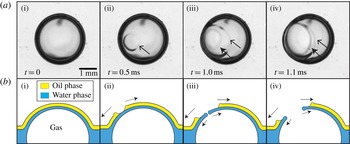
In some experimental scenarios, Feng et al. (Reference Feng, Roché, Vigolo, Arnaudov, Stoyanov, Gurkov, Tsutsumanova and Stone2014) observed simultaneous rupture of the oil and water layers. However, in others they observed rupture of the distinct films of oil and water separately: the oil layer ruptures first, retracting across the water layer beneath, which is then followed by the rupture of the water layer; we refer to such dynamics as ‘separated rupture’. This process is illustrated in the four panels of figure 1. The origin of the distinct rupture behaviour has not been studied to the best of our knowledge, but the authors speculated that it may be due to a combination of the presence of surfactant and fluid wettability, with rupture almost always occurring simultaneously in the absence of surfactant and for completely wetting fluids. In this paper we present a theoretical model for this canonical two-layer system that provides predictions for the possible mechanism of separated rupture, the parameter regimes for which we expect separated rupture and those when simultaneous rupture should take place. The results of our analysis of this model problem provide indications of the role that various features might play in more complex, physically relevant, scenarios such as the bubble bursting in oil spills mentioned in Feng et al. (Reference Feng, Roché, Vigolo, Arnaudov, Stoyanov, Gurkov, Tsutsumanova and Stone2014).
(a) Plan-view photos in time sequence for the bursting of a bubble at interfaces of air/hexadecane/water at
 $[\text{C}_{16}\text{TAB}]=0.09~\text{mM}$
(the oil layer thickness is 1 mm and the scale bar is 1 mm) and (b) corresponding side-view schematics: (i) a bubble deforms the compound air–liquid interfaces; (ii) the oil film ruptures forming a nucleation hole, highlighted with an arrow; (iii) the water films ruptures forming a second nucleation hole, highlighted by a filled arrow; (iv) two different retracting liquid rims are then observed simultaneously.

The canonical configuration comprises a rising bubble in a bath of water, which is covered with a thin layer of oil. As the bubble approaches the surface it rapidly decelerates as it begins to deflect the oil–water interface, trapping a water film between the bubble and the oil layer. This scenario can be modelled as a two-layer liquid film confined between the bubble and the atmosphere (figure 2
a). As the bubble continues to rise, the liquid films thin and attractive van der Waals forces between the interfaces drive an instability that will ultimately rupture the film in finite time. For the system composed of alkanes with an aqueous solution with surfactant
 $\text{C}_{n}\text{TAB}$
, typically the oil film is observed to rupture first, which then retracts over the aqueous film beneath, with the aqueous layer rupturing up to several hundreds of milliseconds later (Feng et al.
Reference Feng, Roché, Vigolo, Arnaudov, Stoyanov, Gurkov, Tsutsumanova and Stone2014).
(a) Schematic of the physical system. (b) Model set-up in dimensional variables. The normal and tangent to each interface are denoted by
 $\boldsymbol{n}_{k}$
and
 $\boldsymbol{t}_{k}$
respectively for
 $k=0,1,2$
. The system is characterized by the Cartesian coordinate system
 $(x^{\ast },y^{\ast })$
.

The stability of a single-phase liquid film to intermolecular forces has been investigated for thin films on a substrate (e.g. Williams & Davis Reference Williams and Davis1982; Oron, Davis & Bankoff Reference Oron, Davis and Bankoff1997; Craster & Matar Reference Craster and Matar2009) and free films with two gas–liquid interfaces (Erneux & Davis Reference Erneux and Davis1993). For attractive van der Waals forces, these films are long-wave unstable to small perturbations and the interface profiles are self-similar approaching finite-time rupture (Witelski & Bernoff Reference Witelski and Bernoff1999; Zhang & Lister Reference Zhang and Lister1999; Vaynblat, Lister & Witelski Reference Vaynblat, Lister and Witelski2001). Similar ideas have also been applied to understand the stability of thinning foam lamellae, where it has been shown that drainage flow along these films is partially stabilizing (Anderson, Brush & Davis Reference Anderson, Brush and Davis2010; Davis, Stewart & Davis Reference Davis, Stewart and Davis2013).
The stability of a bi-layer liquid film on a solid substrate (with two fluid–fluid interfaces) bears many similarities to the experimental system outlined above, where the layers can exhibit dewetting and rupture, with application to the flow of mucus on the lining of the airways (Craster & Matar Reference Craster and Matar2000; Matar, Craster & Warner Reference Matar, Craster and Warner2002), the tear film (Zhang, Matar & Craster Reference Zhang, Matar and Craster2003) or industrial coating processes (Pototsky et al. Reference Pototsky, Bestehorn, Merkt and Thiele2004, Reference Pototsky, Bestehorn, Merkt and Thiele2005; Fisher & Golovin Reference Fisher and Golovin2005). The stability of this bi-layer system to van der Waals attractions has been widely studied, where the system exhibits two temporal branches, one or both of which can be unstable (Pototsky et al. Reference Pototsky, Bestehorn, Merkt and Thiele2004; Fisher & Golovin Reference Fisher and Golovin2005). In addition, the uniform state admits both sinuous (zigzag) and varicose perturbation modes, where the perturbed interfaces are in phase or in antiphase respectively. Fully nonlinear simulations elucidated that the film ruptures distinctly in either the upper layer or the lower layer (Pototsky et al. Reference Pototsky, Bestehorn, Merkt and Thiele2004) but also demonstrated the existence of periodic (non-uniform) solutions that coarsen in time (Pototsky et al. Reference Pototsky, Bestehorn, Merkt and Thiele2005, Reference Pototsky, Bestehorn, Merkt and Thiele2006). Further analysis of this system also uncovered oscillatory dewetting behaviour in the presence of surfactants (Fisher & Golovin Reference Fisher and Golovin2007), while a classification of the distinct rupture modes was made by Ward (Reference Ward2011). The governing equations derived in these studies are similar to one class of equations presented herein (equations (4.10) below) for a bi-layer free film with an abundance of surfactant on the air–aqueous interface.
In this paper we present a canonical model that captures the key dynamical features of a bi-layer free liquid film to characterize its rupture under van der Waals forces, where the resulting system possesses three fluid–fluid interfaces (figure 2 a). In particular, we consider the case where both layers experience a non-retarded (attractive) van der Waals force between the interfaces so as to isolate parameter regimes and interfacial conditions for which either both layers rupture simultaneously or the two layers rupture distinctly, which provides insight into the role of surfactant and wettability on the rupture mechanics. We choose to study a simplified geometry comprising two liquid films with a common interface, surrounded on both sides by a passive gas, which captures the key features of the final stages of bubble bursting considered in Feng et al. (Reference Feng, Roché, Vigolo, Arnaudov, Stoyanov, Gurkov, Tsutsumanova and Stone2014). Here, the gas beneath the films may be identified with a rising bubble in the liquid while the gas above corresponds to the surrounding atmosphere (figure 2 a). This model simplification allows us to examine the planar geometry illustrated in figure 2(b), where the difference in pressure between the bubble and the atmosphere is assumed negligible, and large-scale film bending can be ignored. The resulting set-up provides a tractable model that is amenable to mathematical analysis, and offers a foundation to provide insights into the response of corresponding physical systems.
The mathematical model for the full system is presented in § 2. In §§ 3 and 4 we exploit the slenderness of the geometry to reduce the governing equations to a coupled system of one-dimensional partial differential equations. In particular, we study two distinct regimes: one that models an oil-covered clean water film (§ 3) and the second that mimics water containing an abundance of surfactant (§ 4). We examine the stability of each configuration via linear stability analysis and full numerical simulations, allowing us to explore the features necessary to induce distinct film rupture. In § 5 we reconcile our predictions with the original experimental set-up and in § 6 we draw conclusions on the implications of our model for practical scenarios.
2. Mathematical modelling
2.1. Dimensional model equations and boundary conditions
We examine a model set-up of a planar free liquid film composed of two long and thin immiscible fluid layers, shown in figure 2(b), surrounded on both sides by a passive gas of constant pressure
 $p_{0}^{\ast }$
. We denote the lower layer as liquid 1 (water in the experiment) and the upper layer as liquid 2 (oil in the experiment). Both layers are assumed to be Newtonian liquids of viscosity
 ${\it\mu}_{j}~(j=1,2)$
and the flows are assumed to be incompressible. In the spirit of our assumption of a long slender geometry, we also neglect any effects that may arise due to large-scale film bending, and the resulting pressure differences that may arise. The system has three fluid–fluid interfaces denoted by
 $k=0,1,2$
, with associated surface-tension coefficients
 ${\it\gamma}_{k}$
: the interface between liquid 1 and liquid 2 is denoted as
 $k=0$
, the interface between liquid 1 and the gas is denoted as
 $k=1$
and the interface between liquid 2 and the gas is denoted as
 $k=2$
(figure 2
b). We assume that the surface-tension coefficients are all constant, but will use the boundary condition on the liquid 1–gas interface to mimic the presence or absence of surfactant adsorbed from the water phase.
We employ a two-dimensional Cartesian coordinate system, where
 $x^{\ast }$
denotes the (dimensional) displacement along the flat interface 0 profile and
 $y^{\ast }$
denotes the distance normal to this direction with direction into fluid 2 (figure 2
b). We denote interface 0 (between the two liquids) as
 $y^{\ast }=H^{\ast }(x^{\ast },t^{\ast })$
, interface 1 as
 $y^{\ast }=H^{\ast }(x^{\ast },t^{\ast })-h_{1}^{\ast }(x^{\ast },t^{\ast })$
and interface 2 as
 $y^{\ast }=H^{\ast }(x,t)+h_{2}^{\ast }(x,t)$
, and the corresponding normal and tangent unit vectors along these interfaces as
 $\boldsymbol{n}_{k}$
and
 $\boldsymbol{t}_{k}~(k=0,1,2)$
respectively, also illustrated in figure 2(b).
The velocity and pressure fields in liquids 1 and 2 are denoted as
 $\boldsymbol{u}_{j}^{\ast }=(u_{j}^{\ast },v_{j}^{\ast })$
and
 $p_{j}^{\ast }$
respectively (
 $j=1,2$
). Throughout this study we neglect inertial and gravitational effects, so the flow is governed by the Stokes equations in both fluids,
 $$\begin{eqnarray}\displaystyle & \boldsymbol{{\rm\nabla}}^{\ast }\boldsymbol{\cdot }\boldsymbol{u}_{1}^{\ast }=0,\quad \boldsymbol{{\rm\nabla}}^{\ast }p_{1}^{\ast }={\it\mu}_{1}{{\rm\nabla}^{\ast }}^{2}\boldsymbol{u}_{1}^{\ast },\quad H^{\ast }-h_{1}^{\ast }<y^{\ast }<H^{\ast }, & \displaystyle\end{eqnarray}$$
 $$\begin{eqnarray}\displaystyle & \boldsymbol{{\rm\nabla}}^{\ast }\boldsymbol{\cdot }\boldsymbol{u}_{2}^{\ast }=0,\quad \boldsymbol{{\rm\nabla}}^{\ast }p_{2}^{\ast }={\it\mu}_{2}{{\rm\nabla}^{\ast }}^{2}\boldsymbol{u}_{2}^{\ast },\quad H^{\ast }<y^{\ast }<H^{\ast }+h_{2}^{\ast }. & \displaystyle\end{eqnarray}$$
 $$\begin{eqnarray}{\bf\sigma}_{1}^{\ast }=-p_{1}^{\ast }\unicode[STIX]{x1D644}+{\it\mu}_{1}(\boldsymbol{{\rm\nabla}}^{\ast }\boldsymbol{u}_{1}^{\ast }+(\boldsymbol{{\rm\nabla}}^{\ast }\boldsymbol{u}_{1}^{\ast })^{\text{T}}),\quad {\bf\sigma}_{2}^{\ast }=-p_{2}^{\ast }\unicode[STIX]{x1D644}+{\it\mu}_{2}(\boldsymbol{{\rm\nabla}}^{\ast }\boldsymbol{u}_{2}^{\ast }+(\boldsymbol{{\rm\nabla}}^{\ast }\boldsymbol{u}_{2}^{\ast })^{\text{T}}).\end{eqnarray}$$
Each gas–liquid interface (
 $k=0,1,2$
) experiences a van der Waals force of attraction to/repulsion from the other two interfaces in the system. In accordance with many other studies on the stability of thin liquid films (reviewed by Oron et al.
Reference Oron, Davis and Bankoff1997; Craster & Matar Reference Craster and Matar2009), we approximate this force as the interaction between two flat parallel interfaces (valid in the long-wavelength limit we adopt below); following Israelachvili (Reference Israelachvili2011), this force is proportional to the Hamaker constant of interaction between the two interfaces (which may be positive or negative) and inversely proportional to the cube of the perpendicular distance between these interfaces. In this study we define an excess pressure
 $\breve{p}_{j}^{\ast }~(j=1,2)$
which (by definition) shifts the influence of the van der Waals forces from the normal stress boundary conditions to the bulk liquid (essentially appearing as a body force on the system). Such an approach has been used widely in previous studies (e.g. Patzer & Homsy Reference Patzer and Homsy1975; Matar et al.
Reference Matar, Craster and Warner2002). In this case, the excess pressure is defined via
 $$\begin{eqnarray}\displaystyle & p_{j}^{\ast }=\breve{p}_{j}^{\ast }+{\it\phi}_{j}^{\ast }\quad (j=1,2), & \displaystyle\end{eqnarray}$$
where the Stokes equations in both fluids (2.1) can be written as
 $$\begin{eqnarray}\displaystyle & \boldsymbol{{\rm\nabla}}^{\ast }\boldsymbol{\cdot }\boldsymbol{u}_{1}^{\ast }=0,\quad \boldsymbol{{\rm\nabla}}^{\ast }(\breve{p}_{1}^{\ast }+{\it\phi}_{1}^{\ast })={\it\mu}_{1}{{\rm\nabla}^{\ast }}^{2}\boldsymbol{u}_{1}^{\ast },\quad H^{\ast }-h_{1}^{\ast }<y^{\ast }<H^{\ast }, & \displaystyle\end{eqnarray}$$
 $$\begin{eqnarray}\displaystyle & \boldsymbol{{\rm\nabla}}^{\ast }\boldsymbol{\cdot }\boldsymbol{u}_{2}^{\ast }=0,\quad \boldsymbol{{\rm\nabla}}^{\ast }(\breve{p}_{2}^{\ast }+{\it\phi}_{2}^{\ast })={\it\mu}_{2}{{\rm\nabla}^{\ast }}^{2}\boldsymbol{u}_{2}^{\ast },\quad H^{\ast }<y^{\ast }<H^{\ast }+h_{2}^{\ast }, & \displaystyle\end{eqnarray}$$
where
 ${\it\phi}_{j}^{\ast }$
are van der Waals potentials for layer
 $j~(j=1,2)$
defined according to
 $$\begin{eqnarray}\displaystyle & \displaystyle {\it\phi}_{1}^{\ast }=\frac{A_{1}}{6{\rm\pi}{h_{1}^{\ast }}^{3}}+\frac{A_{2}}{6{\rm\pi}(h_{1}^{\ast }+h_{2}^{\ast })^{3}},\quad {\it\phi}_{2}^{\ast }=\frac{A_{3}}{6{\rm\pi}{h_{2}^{\ast }}^{3}}+\frac{A_{4}}{6{\rm\pi}(h_{1}^{\ast }+h_{2}^{\ast })^{3}}, & \displaystyle\end{eqnarray}$$
where
 $A_{1},\dots ,A_{4}$
are Hamaker constants. This description is consistent with the van der Waals pressure used by Matar et al. (Reference Matar, Craster and Warner2002), and the Hamaker constants can be derived using the method outlined by Pototsky et al. (Reference Pototsky, Bestehorn, Merkt and Thiele2005). If the gas on both sides of the film is the same then the two Hamaker constants
 $A_{2}$
and
 $A_{4}$
are identical, which we assume throughout this study. To promote rupture, in the analysis in §§ 3 and 4 we consider only non-retarded van der Waals forces, and so these Hamaker constants are assumed to be non-negative. In § 5 we relax this constraint and consider the effect of repulsive van der Waals forces. We henceforth drop breves ( ̆ ) on the pressure terms for notational convenience.
On interface 0 we impose a kinematic condition as well as continuity of velocity, and normal and tangential stresses in the form
 $$\begin{eqnarray}\displaystyle & u_{1}^{\ast }=u_{2}^{\ast },\quad v_{1}^{\ast }=v_{2}^{\ast }=H_{t^{\ast }}^{\ast }+u_{1}^{\ast }H_{x^{\ast }}^{\ast },\quad {\bf\sigma}_{2}^{\ast }\boldsymbol{\cdot }\boldsymbol{n}_{0}-{\bf\sigma}_{1}^{\ast }\boldsymbol{\cdot }\boldsymbol{n}_{0}={\it\gamma}_{0}{\it\kappa}_{0}^{\ast }\boldsymbol{n}_{0},\quad \text{on}~y^{\ast }=H^{\ast },\qquad & \displaystyle\end{eqnarray}$$
where
 ${\it\kappa}_{0}^{\ast }=\boldsymbol{{\rm\nabla}}_{s0}\boldsymbol{\cdot }\boldsymbol{n}_{0}$
is the mean curvature of the interface
 $y^{\ast }=H^{\ast }(x^{\ast },t^{\ast })$
, where
 $\boldsymbol{{\rm\nabla}}_{sj}=(\unicode[STIX]{x1D644}-\boldsymbol{n}_{j}\boldsymbol{n}_{j})\boldsymbol{\cdot }\boldsymbol{{\rm\nabla}}$
is the surface gradient operator on interface
 $j$
, and subscripts
 $x^{\ast }$
,
 $t^{\ast }$
denote differentiation.
On interface 1 we impose kinematic conditions and continuity of normal stress respectively, in the form
 $$\begin{eqnarray}\displaystyle v_{1}^{\ast }=(H^{\ast }-h_{1}^{\ast })_{t^{\ast }}+u_{1}^{\ast }(H^{\ast }-h_{1}^{\ast })_{x^{\ast }},\quad p_{0}^{\ast }+\boldsymbol{n}_{1}\boldsymbol{\cdot }{\bf\sigma}_{1}^{\ast }\boldsymbol{\cdot }\boldsymbol{n}_{1}={\it\gamma}_{1}{\it\kappa}_{1}^{\ast },\quad \text{on}~y^{\ast }=H^{\ast }-h_{1}^{\ast },\qquad & & \displaystyle\end{eqnarray}$$
where
 ${\it\kappa}_{1}^{\ast }=\boldsymbol{{\rm\nabla}}_{s1}\boldsymbol{\cdot }\boldsymbol{n}_{1}$
is the mean curvature of the interface
 $y^{\ast }=H^{\ast }(x^{\ast },t^{\ast })-h_{1}^{\ast }(x^{\ast },t^{\ast })$
. One final interfacial condition is required, which we use to express the presence (or absence) of surfactant. For example, in follow-up experiments it is observed that surfactant must be present in the water phase for multiple rupture events to occur. To validate this observation, in this paper we shall examine two distinct cases, namely
-
(i) zero tangential stress,
(2.4c )to represent a surfactant-free interface (air–aqueous phase); or $$\begin{eqnarray}\displaystyle & \boldsymbol{t}_{1}\boldsymbol{\cdot }{\bf\sigma}_{1}^{\ast }\boldsymbol{\cdot }\boldsymbol{n}_{1}=0,\quad \text{on}~y^{\ast }=H^{\ast }-h_{1}^{\ast }, & \displaystyle\end{eqnarray}$$
-
(ii) a tangentially immobile surface,
(2.4d )
$$\begin{eqnarray}\displaystyle & \boldsymbol{u}_{1}^{\ast }\boldsymbol{\cdot }\boldsymbol{t}_{1}=0,\quad \text{on}~y^{\ast }=H^{\ast }-h_{1}^{\ast }, & \displaystyle\end{eqnarray}$$


to represent a surfactant-saturated air–aqueous interface. This assumption follows a number of previous theoretical studies examining the microscale flow in surfactant-saturated foam films (for example Patzer & Homsy Reference Patzer and Homsy1975; Schwartz & Princen Reference Schwartz and Princen1987). This equates to assuming that the surface elastic modulus of the surfactant-laden interface is large, consistent with experimental observations that the creation of an interface in an extending soap foam lamella is restricted to a narrow region at the edge of the elongating film (Mysels & Cox Reference Mysels and Cox1962).
We acknowledge that the effect of surfactant at a fluid boundary can be characterized in a variety of ways with differing complexity. For instance, in some applications ‘remobilizing surfactants’ can allow for interfacial flow in a surfactant-loaded interface, and it becomes necessary to explicitly track surfactant monomer and micelle concentrations (Stebe & Maldarelli Reference Stebe and Maldarelli1994). However, we choose these two distinct boundary conditions to exemplify two contrasting limits in the simplest possible way.
On interface 2 we impose kinematic conditions and continuity of normal and tangential stress respectively, in the form
 $$\begin{eqnarray}\displaystyle & v_{2}^{\ast }=(H^{\ast }+h_{2}^{\ast })_{t^{\ast }}+u_{2}^{\ast }(H^{\ast }+h_{2}^{\ast })_{x^{\ast }},\quad \boldsymbol{n}_{2}\boldsymbol{\cdot }p_{0}^{\ast }+{\bf\sigma}_{2}^{\ast }\boldsymbol{\cdot }\boldsymbol{n}_{2}={\it\gamma}_{2}{\it\kappa}_{2}^{\ast }\boldsymbol{n}_{2},\quad \text{on}~y^{\ast }=H^{\ast }+h_{2}^{\ast }, & \displaystyle \nonumber\\ \displaystyle & & \displaystyle\end{eqnarray}$$
where
 ${\it\kappa}_{2}^{\ast }=\boldsymbol{{\rm\nabla}}_{s2}\boldsymbol{\cdot }\boldsymbol{n}_{2}$
is the mean curvature of the interface
 $y^{\ast }=H^{\ast }(x^{\ast },t^{\ast })+h_{2}^{\ast }(x^{\ast },t^{\ast })$
.
Since the external gas pressure on both sides of the bi-layer has been assumed as
 $p_{0}^{\ast }$
, this formulation implicitly neglects the pressure drop due to the curvature of the bubble that would be present in the experiments of Feng et al. (Reference Feng, Roché, Vigolo, Arnaudov, Stoyanov, Gurkov, Tsutsumanova and Stone2014).
2.2. Non-dimensionalization and scaling
Just prior to rupture, when the bubble is close to the surface, the liquid layers are typically much longer than their thickness. We exploit this film slenderness to reduce the governing equations via a systematic asymptotic analysis (Erneux & Davis Reference Erneux and Davis1993). We shall assume that we begin with two viscous films whose thicknesses are initially uniform and comparable but not necessarily equal in magnitude, and define
 ${\it\epsilon}\ll 1$
as the ratio of the initial thickness of fluid 1 to a characteristic axial extent,
 $L$
. The natural scaling choice is then
 $$\begin{eqnarray}(x^{\ast },y^{\ast })=L(x,{\it\epsilon}y),\quad \boldsymbol{u}^{\ast }=(u^{\ast },v^{\ast })=U_{0}(u,{\it\epsilon}v),\quad t^{\ast }=\frac{L}{U_{0}}t,\end{eqnarray}$$
 $$\begin{eqnarray}p^{\ast }=p_{0}^{\ast }+\left(\frac{{\it\mu}_{1}U_{0}}{L}\right)p,\quad H^{\ast }={\it\epsilon}LH,\quad h^{\ast }={\it\epsilon}Lh,\end{eqnarray}$$
where
 $U_{0}$
is a typical axial velocity.
If we select
 $U_{0}={\it\epsilon}{\it\gamma}_{0}/{\it\mu}_{1}$
then the remaining six dimensionless parameters that appear in the resulting dimensionless equations in addition to the small parameter
 ${\it\epsilon}$
are
 $$\begin{eqnarray}\displaystyle & \displaystyle \overline{{\it\mu}}=\frac{{\it\mu}_{2}}{{\it\mu}_{1}},\quad \mathscr{C}_{j}=\frac{{\it\gamma}_{j}}{{\it\gamma}_{0}}\quad (j=1,2),\quad \mathscr{A}_{n}=\frac{1}{{\it\epsilon}^{4}}\frac{A_{n}}{6{\rm\pi}{\it\gamma}_{0}L^{2}}\quad (n=1,\dots ,3), & \displaystyle\end{eqnarray}$$
denoting respectively the viscosity contrast between the two layers, the surface-tension contrast between interface 0 and interfaces 1 and 2 and the three dimensionless Hamaker constants. In § 5 we estimate each of these parameters for the experiments of Feng et al. (Reference Feng, Roché, Vigolo, Arnaudov, Stoyanov, Gurkov, Tsutsumanova and Stone2014).
In dimensionless form the initial (uniform) film thicknesses can be written as
 $$\begin{eqnarray}h_{1}(x,0)=1,\quad h_{2}(x,0)=\overline{h}_{2},\end{eqnarray}$$
where
 $\overline{h}_{2}$
is an order-one constant and corresponds to the initial ratio of the thicknesses of the two films.
Our subsequent analysis will be arranged into three sections. We begin in § 3 by considering the regime in which no tangential stress is exerted on interface 1, (2.4c ), to analyse the potential rupture behaviour that may be observed in the absence of surfactant within the water film. In § 4 we address the case where the water phase contains an abundance of surfactant adsorbed on the air–liquid interface, by assuming a tangentially immobile interface, (2.4d ). In both sections our aim is to identify conditions where the bi-layer free film is unstable, and determine whether that instability will lead to an isolated dewetting event, that is, dewetting in one layer only, or the dewetting of both layers simultaneously. In § 5 we reconcile these predictions with the experiments of Feng et al. (Reference Feng, Roché, Vigolo, Arnaudov, Stoyanov, Gurkov, Tsutsumanova and Stone2014).
The dimensionless van der Waals pressures can be written as
 $$\begin{eqnarray}{\it\phi}_{1}=\frac{\mathscr{A}_{1}}{{h_{1}}^{3}}+\frac{\mathscr{A}_{2}}{(h_{1}+h_{2})^{3}},\quad {\it\phi}_{2}=\frac{\mathscr{A}_{3}}{{h_{2}}^{3}}+\frac{\mathscr{A}_{2}}{(h_{1}+h_{2})^{3}}.\end{eqnarray}$$
To avoid an abundance of parameters and lengthy expressions, in §§ 3 and 4 below we neglect the attraction between the two outer interfaces by setting
 $\mathscr{A}_{2}=0$
throughout: since
 $h_{1}$
and
 $h_{2}$
are always positive, for comparable Hamaker constants this component of the pressure must always be weaker that the attraction between the two interfaces adjacent to that layer, and so we expect the rupture behaviour to be well characterized by the first terms in
 ${\it\phi}_{j}~(j=1,2)$
. However, a more complete discussion of the Hamaker constants will be given in § 5 where we use the full expression for the van der Waals pressure (2.9), as we find that some of these Hamaker constants can be negative in the experimental regime of Feng et al. (Reference Feng, Roché, Vigolo, Arnaudov, Stoyanov, Gurkov, Tsutsumanova and Stone2014).
3. A surfactant-free interface
3.1. Governing equations
In the absence of surfactant in the water phase we must solve the dimensionless version of (2.1) subject to the dimensionless versions of the boundary conditions (2.4a
)–(2.4c
) and (2.4e
). We exploit the long thin geometry in our problem by considering the limit
 ${\it\varepsilon}\rightarrow 0$
, and expanding all dependent variables in power series of the form
 $$\begin{eqnarray}{\it\psi}={\it\psi}^{(0)}+{\it\epsilon}^{2}{\it\psi}^{(2)}+\cdots \,.\end{eqnarray}$$
At leading order the governing equations become, dropping the ‘
 $(0)$
’ superscripts for clarity,
 $$\begin{eqnarray}\displaystyle & \boldsymbol{{\rm\nabla}}\boldsymbol{\cdot }\boldsymbol{u}_{1}=0,\quad u_{1,yy}=0,\quad p_{1,y}+{\it\phi}_{1,y}=v_{1,yy},\quad H-h_{1}<y<H, & \displaystyle\end{eqnarray}$$
 $$\begin{eqnarray}\displaystyle & \boldsymbol{{\rm\nabla}}\boldsymbol{\cdot }\boldsymbol{u}_{2}=0,\quad u_{2,yy}=0,\quad p_{2,y}+{\it\phi}_{2,y}=\overline{{\it\mu}}v_{2,yy},\quad H<y<H+h_{2}, & \displaystyle\end{eqnarray}$$
and we also state the leading-order boundary conditions,
 $$\begin{eqnarray}v_{1}=(H-h_{1})_{t}+u_{1}(H-h_{1})_{x},\quad u_{1,y}=0,\quad -p_{1}+2v_{1,y}=-\mathscr{C}_{1}(H-h_{1})_{xx},\end{eqnarray}$$
on
 $y=H-h_{1}$
,
 $$\begin{eqnarray}\displaystyle & & \displaystyle u_{1}=u_{2},\quad v_{1}=v_{2}=H_{t}+u_{1}H_{x},\quad \overline{{\it\mu}}u_{2,y}=u_{1,y},\quad \nonumber\\ \displaystyle & & \displaystyle \qquad -p_{2}+2\overline{{\it\mu}}v_{2,y}+p_{1}-2v_{1,y}=-H_{xx},\end{eqnarray}$$
on
 $y=H$
and
 $$\begin{eqnarray}\displaystyle & v_{2}=(H+h_{2})_{t}+u_{2}(H+h_{2})_{x},\quad u_{2,y}=0,\quad -p_{2}+2\overline{{\it\mu}}v_{2,y}=\mathscr{C}_{2}(H+h_{2})_{xx}, & \displaystyle\end{eqnarray}$$
on
 $y=H+h_{2}$
.
We observe that neither
 $u_{1}$
nor
 $u_{2}$
depends on
 $y$
, so we have the same uniform plug flow in both films,
 $u_{1}=u_{2}=U(x,t)$
, similar to models of draining foam lamellae (Breward & Howell Reference Breward and Howell2002; Brush & Davis Reference Brush and Davis2005) and other problems bounded by free surfaces (see, for example, Eggers Reference Eggers1997). Integrating the continuity equations over the film thickness yields the depth-averaged continuity equations
 $$\begin{eqnarray}\displaystyle & h_{1,t}+(Uh_{1})_{x}=0, & \displaystyle\end{eqnarray}$$
 $$\begin{eqnarray}\displaystyle & h_{2,t}+(Uh_{2})_{x}=0. & \displaystyle\end{eqnarray}$$
Integrating the
 $y$
-component of the Stokes-flow equations in (3.2) over the film thickness and utilizing the pressure boundary conditions in (3.2d,e
) provides a relation between the curvatures of all three interfaces. We then close the problem of solving (3.3) by considering the next-order correction to the
 $x$
-component of the Stokes-flow equations and the tangential component of the dynamic boundary conditions. Our derivation follows closely that found in Erneux & Davis (Reference Erneux and Davis1993) for a single extensional film, although we do not restrict our problem to be symmetric about a midline as they do. We obtain a third and final governing equation of the form
 $$\begin{eqnarray}\displaystyle & & \displaystyle 4((h_{1}+\bar{{\it\mu}}h_{2})U_{x})_{x}-h_{1}{\it\phi}_{1,x}-h_{2}{\it\phi}_{2,x}+h_{1}\mathscr{C}_{1}\frac{(1+\mathscr{C}_{2})h_{1,xxx}+\mathscr{C}_{2}h_{2,xxx}}{1+\mathscr{C}_{1}+\mathscr{C}_{2}}\nonumber\\ \displaystyle & & \displaystyle \qquad +\,h_{2}\mathscr{C}_{2}\frac{(1+\mathscr{C}_{1})h_{2,xxx}+\mathscr{C}_{1}h_{1,xxx}}{1+\mathscr{C}_{1}+\mathscr{C}_{2}}=0.\end{eqnarray}$$
It should be noted that if we set
 $h_{1}=\mathscr{H}h_{2}$
, where
 $\mathscr{H}$
is a constant, the conservation of mass equations for layers 1 and 2 (3.3a,b
) become identical and the system (3.3) reduces to two coupled partial differential equations (PDEs). However, we consider the full system in the analysis below.
We notice that (3.3c ) can be written more succinctly as
 $$\begin{eqnarray}\displaystyle & h_{1}\overline{p}_{1,x}+h_{2}\overline{p}_{2,x}-4((h_{1}+\overline{{\it\mu}}h_{2})U_{x})_{x}=0, & \displaystyle\end{eqnarray}$$
where we define
 $$\begin{eqnarray}\displaystyle & \displaystyle \overline{p}_{1}=-\mathscr{C}_{1}\frac{(1+\mathscr{C}_{2})h_{1,xx}+\mathscr{C}_{2}h_{2,xx}}{1+\mathscr{C}_{1}+\mathscr{C}_{2}}+{\it\phi}_{1}, & \displaystyle\end{eqnarray}$$
 $$\begin{eqnarray}\displaystyle & \displaystyle \overline{p}_{2}=-\mathscr{C}_{2}\frac{(1+\mathscr{C}_{1})h_{2,xx}+\mathscr{C}_{1}h_{1,xx}}{1+\mathscr{C}_{1}+\mathscr{C}_{2}}+{\it\phi}_{2} & \displaystyle\end{eqnarray}$$
as modified pressures. Equations (3.3) are the bi-layer equivalents of the free-film equations of Erneux & Davis (Reference Erneux and Davis1993) for two extensional thin films. The bi-layer midline satisfies
 $$\begin{eqnarray}H_{xx}=\frac{\mathscr{C}_{1}h_{1,xx}-\mathscr{C}_{2}h_{2,xx}}{1+\mathscr{C}_{1}+\mathscr{C}_{2}},\end{eqnarray}$$
which can be calculated directly once
 $h_{1}$
and
 $h_{2}$
are known, given suitable boundary conditions.
3.2. Linear stability analysis
To begin with we shall explore the features that characterize the onset of instability by performing a linear stability analysis. The governing equations (3.3) admit a uniform solution in which there is no flow and both films are of constant thickness. We perturb the system about this state by posing the expansions
 $$\begin{eqnarray}(h_{1},h_{2},U)=(1,\overline{h}_{2},0)+(1,h_{2}^{\prime },U^{\prime }){\it\delta}\exp ({\it\omega}t+\text{i}kx),\end{eqnarray}$$
where
 $|{\it\delta}|\ll 1$
.
Development of an initial perturbation of the form (3.10) with fixed wavenumber
 $k={\rm\pi}$
,
 $\mathscr{C}_{1}=\mathscr{C}_{2}=1$
,
 $\overline{{\it\mu}}=2$
,
 ${\it\delta}=0.01$
and
 $h_{2}^{\prime }$
and
 $U^{\prime }$
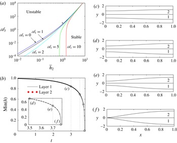
determined by (3.7). (a) Neutral stability curves ((3.8) with
 ${\it\omega}=0$
) in the parameter space spanned by
 $\mathscr{A}_{3}$
and
 $\overline{h}_{2}$
for
 $\mathscr{A}_{1}=0,1,2,5,10$
. The uniform state is stable to the right of the curves and unstable to the left. The fully nonlinear simulations of (3.3) shown in (c–f) are conducted at the point marked with a cross. (b) Temporal evolution of the minimum thickness in both layers with
 $\mathscr{A}_{1}=0$
and
 $\mathscr{A}_{3}=1$
. The inset shows a close-up of the approach to rupture. (c–f) Snapshots of the two layers at various times illustrating the evolution towards simultaneous rupture, with the corresponding times marked on (b) ((c)
 $t=3.000$
; (d)
 $t=3.500$
; (e)
 $t=3.700$
; (f)
 $t=3.769$
).

Expanding (3.3a,b
) at
 $O({\it\delta})$
we find that
 $$\begin{eqnarray}U^{\prime }=\text{i}{\it\omega}/k,\quad h_{2}^{\prime }=\overline{h}_{2}>0,\end{eqnarray}$$
and thus, in the absence of surfactant, any deviations in the interface are varicose in nature. Similarly, writing (3.3c
) at
 $O({\it\delta})$
and using (3.7) we obtain the dispersion relation
 $$\begin{eqnarray}{\it\omega}=\frac{3(\overline{h}_{2}^{2}\mathscr{A}_{1}+\mathscr{A}_{3})}{4\overline{h}_{2}^{2}(1+\overline{{\it\mu}}\overline{h}_{2})}-\frac{(\mathscr{C}_{2}\overline{h}_{2}^{2}+\mathscr{C}_{1}(1+\mathscr{C}_{2}(1+\overline{h}_{2})^{2}))}{4(1+\bar{{\it\mu}}\overline{h}_{2})(1+\mathscr{C}_{1}+\mathscr{C}_{2})}k^{2}.\end{eqnarray}$$
We note that as
 $k\rightarrow \infty$
,
 ${\it\omega}\rightarrow -\infty$
, so short-wavelength perturbations are stable. However, we also observe that there is a possibility for
 ${\it\omega}>0$
, leading to instabilities if
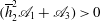 $(\overline{h}_{2}^{2}\mathscr{A}_{1}+\mathscr{A}_{3})>0$
. If
 $\mathscr{A}_{1}$
and
 $\mathscr{A}_{3}$
are non-negative (non-retarded van der Waals) then this constraint is always satisfied. (We explore the influence of repulsive van der Waals in § 5.) All wavenumbers
 $k>k_{crit}$
will be stable, where
 $$\begin{eqnarray}k_{crit}=\sqrt{\frac{3(1+\mathscr{ C}_{1}+\mathscr{ C}_{2})(\overline{h}_{2}^{2}\mathscr{A}_{1}+\mathscr{ A}_{3})}{\overline{h}_{2}^{2}(\mathscr{C}_{2}\overline{h}_{2}^{2}+\mathscr{C}_{1}(1+\mathscr{C}_{2}(1+\overline{h}_{2})^{2}))}}.\end{eqnarray}$$
For disturbances of fixed wavenumber
 $k={\rm\pi}$
(the shortest wavelength to fit into the finite domain
 $-1\leqslant x\leqslant 1$
considered in § 3.3 below), the neutral stability curves (
 $\text{Re}({\it\omega})=0$
) in the space spanned by
 $\mathscr{A}_{3}$
and
 $\overline{h}_{2}$
are shown in figure 3(a) for various values of
 $\mathscr{A}_{1}$
. The uniform state is stable to the right of these curves and unstable otherwise. The dimensionless Hamaker constants
 $\mathscr{A}_{1}$
and
 $\mathscr{A}_{3}$
appear additively in the dispersion relation (3.8) and stability criteria (3.9), so the system can exhibit instability even when van der Waals attractions act in one layer only.
We thus see that the system is unstable only in certain parameter regimes. More importantly, (3.7) indicates that any instabilities will be varicose, and a thinning of one film is necessarily coupled to thinning of the second film even when van der Waals forces act in only one of the layers.
3.3. Nonlinear rupture
To examine the growth of the linear instabilities towards dewetting of one or more of the liquid layers we must consider the full nonlinear system (3.3). The spatial derivatives are discretized using fourth-order centred finite differences, and the resulting system of ordinary differential equations and algebraic constraints is solved numerically using ode15s in MATLAB.
For computational practicality we consider a finite periodic domain
 $-1\leqslant x\leqslant 1$
(corresponding to
 $k={\rm\pi}$
in the linear stability analysis) to ensure that we continue to apply the most passive end constraints on the system, so that any observed phenomenon is induced by the bulk fluid behaviour and the interfacial boundary conditions. We further reduce the problem by assuming that the interface profiles are symmetric about
 $x=0$
, which requires no flow across
 $x=0$
. Since our aim is to examine scenarios where we observe dewetting in one layer and not in the other, we consider a regime in which van der Waals destabilizing forces act in fluid 2 but not in fluid 1 (
 $\mathscr{A}_{1}=0$
). We then examine the nonlinear growth of a sinusoidal varicose initial perturbation
 $$\begin{eqnarray}(h_{1},h_{2},U)=(1,\overline{h}_{2},0)+{\it\delta}\text{Re}[(1,h_{2}^{\prime },U^{\prime })\exp (\text{i}kx)],\end{eqnarray}$$
where
 $h_{2}^{\prime }$
and
 $U^{\prime }$
follow from the linear stability analysis in § 3.2. In all the numerical simulations discussed below we set
 ${\it\delta}=0.01$
, but this choice makes no qualitative difference to the behaviour.
The initial perturbation is observed to grow, and the thickness of film 2 at the centre of the domain decreases rapidly, approaching a finite-time singularity as a result of the van der Waals attractive forces (time evolution shown in figure 3 b). However, as predicted by the linear stability analysis, the thinning of film 2 drives a simultaneous varicose thinning in film 1, despite the absence of van der Waals forces in that layer (figure 3 c–f). We note that, although the chosen perturbation is varicose, the system is observed to evolve as a varicose instability regardless of the nature of the initial perturbation, corroborating the prediction of the linear stability analysis, (3.7).
The linear stability analysis in § 3.2 suggests that perturbations to the layer thickness
 $h_{2}$
are always a constant multiple,
 $\overline{h}_{2}$
, of
 $h_{1}$
. Given the structure of the nonlinear equations (3.3), we can set
 $h_{2}=\overline{h}_{2}h_{1}$
, upon which the conservation of mass equations for layers 1 and 2 (3.3a,b
) become identical. Hence, layers 1 and 2 must always deform together, and thinning of layer 2 drives thinning in layer 1, so that simultaneous rupture is inevitable.
4. A surfactant-laden interface
When the two liquid–gas interfaces are free of tangential stress (in the absence of surfactant), the two outer interfaces deform in an identical manner and so the two layers must rupture simultaneously. We now proceed to explore the effect of surfactant on the system in an effort to understand the distinct rupture behaviour observed experimentally.
In the presence of an abundance of surfactant that accumulates on interface 1, this interface may be modelled as being tangentially immobile, (2.4d ). We must solve the dimensionless version of (2.1) subject to the dimensionless versions of the boundary conditions (2.4a ), (2.4b ), (2.4d ) and (2.4e ). In this case the shear on interface 1 drives a parabolic flow profile across layer 1.
There are two distinguished limits of interest. First, we consider the asymptotic regime in which layer 2 is much more viscous than layer 1, driving a plug flow in layer 2 (§ 4.1). A similar coupling between a thin film and an extensional film, but on a rigid substrate, was considered by Matar et al. (Reference Matar, Craster and Warner2002) as a model for the two-layer lining of lung airways. Second, we relax the constraint on the viscosity and consider a regime in which the viscosity contrast is of order one. In this case a parabolic flow profile exists in both layers (§ 4.2). This regime is similar to the bi-layer thin films considered by Fisher & Golovin (Reference Fisher and Golovin2005) and Pototsky et al. (Reference Pototsky, Bestehorn, Merkt and Thiele2005), again on a rigid substrate.
In both cases we employ the same non-dimensionalization as in (2.5) and (2.6), with the exception of the scaling for the fluid pressures, for which we use
 $$\begin{eqnarray}p^{\ast }=p_{0}+\left(\frac{{\it\mu}_{1}U_{0}}{{\it\epsilon}^{2}L}\right)\tilde{p}.\end{eqnarray}$$
In contrast to the surfactant-free case, the natural velocity scaling, which reduces the number of free parameters, is now
 $U_{0}={\it\epsilon}^{3}{\it\gamma}_{0}/{\it\mu}_{1}$
.
4.1. Case 1: a large viscosity contrast
4.1.1. Governing equations
A distinguished limit exists when
 $\overline{{\it\mu}}={\it\epsilon}^{-2}\tilde{{\it\mu}}$
, where
 $\tilde{{\it\mu}}$
is of order one. Expansion of all dependent variables according to (3.1) provides the leading-order governing equations, dropping ‘
 $(0)$
’ superscripts for clarity,
 $$\begin{eqnarray}\displaystyle & \boldsymbol{{\rm\nabla}}\boldsymbol{\cdot }\boldsymbol{u}_{1}=0,\quad u_{1,yy}=\tilde{p}_{1,x}+{\it\phi}_{1,x},\quad \tilde{p}_{1,y}+{\it\phi}_{1,y}=0,\quad H-h_{1}<y<H, & \displaystyle\end{eqnarray}$$
 $$\begin{eqnarray}\displaystyle & \boldsymbol{{\rm\nabla}}\boldsymbol{\cdot }\boldsymbol{u}_{2}=0,\quad \tilde{{\it\mu}}u_{2,yy}=0,\quad \tilde{p}_{2,y}+{\it\phi}_{2,y}=\tilde{{\it\mu}}v_{2,yy},\quad H<y<H+h_{2}. & \displaystyle\end{eqnarray}$$
We also restate the leading-order boundary conditions,
 $$\begin{eqnarray}\displaystyle & v_{1}=(H-h_{1})_{t},\quad u_{1}=0,\quad -\tilde{p}_{1}=-\mathscr{C}_{1}(H-h_{1})_{xx}, & \displaystyle\end{eqnarray}$$
on
 $y=H-h_{1}$
,
 $$\begin{eqnarray}\displaystyle & u_{1}=u_{2},\quad v_{1}=v_{2}=H_{t}+u_{1}H_{x},\quad u_{2,y}=0,\quad -\tilde{p}_{2}+2\tilde{{\it\mu}}v_{2,y}+\tilde{p}_{1}=-H_{xx}, & \displaystyle\end{eqnarray}$$
on
 $y=H$
and
 $$\begin{eqnarray}\displaystyle & v_{2}=(H+h_{2})_{t}+u_{2}(H+h_{2})_{x},\quad u_{2,y}=0,\quad -\tilde{p}_{2}+2\tilde{{\it\mu}}v_{2,y}=\mathscr{C}_{2}(H+h_{2})_{xx}, & \displaystyle\end{eqnarray}$$
on
 $y=H+h_{2}$
.
We see immediately that we have a plug flow in layer 2 and introduce
 $U(x,t)=u_{2}(x,y,t)$
. As in § 3, the plug flow velocity along layer 2 is determined by proceeding to next order and accounting for the momentum equation along layer 2, which takes the form
 $$\begin{eqnarray}\displaystyle & \tilde{{\it\mu}}u_{2,yy}^{(2)}=-\tilde{{\it\mu}}u_{2,xx}+\tilde{p}_{2,x}+{\it\phi}_{2,x},\quad H<y<H+h_{2}, & \displaystyle\end{eqnarray}$$
subject to tangential stress boundary conditions
 $$\begin{eqnarray}\displaystyle & \tilde{{\it\mu}}u_{2,y}^{(2)}=u_{1,y}-\tilde{{\it\mu}}v_{2,x}-2\tilde{{\it\mu}}H_{x}(v_{2,y}-u_{2,x}),\quad y=H, & \displaystyle\end{eqnarray}$$
 $$\begin{eqnarray}\displaystyle & u_{2,y}^{(2)}=-v_{2,x}-2(H+h_{2})_{x}(v_{2,y}-u_{2,x}),\quad y=H+h_{2}. & \displaystyle\end{eqnarray}$$
Following the procedure outlined in appendix A of Matar et al. (Reference Matar, Craster and Warner2002), we obtain the governing equations for the two-layer flow,
 $$\begin{eqnarray}\displaystyle & \displaystyle h_{1,t}+\left(\frac{1}{2}h_{1}U-\frac{h_{1}^{3}}{12}\overline{p}_{1,x}\right)_{x}=0, & \displaystyle\end{eqnarray}$$
 $$\begin{eqnarray}\displaystyle & h_{2,t}+(Uh_{2})_{x}=0, & \displaystyle\end{eqnarray}$$
 $$\begin{eqnarray}\displaystyle & \displaystyle 4\tilde{{\it\mu}}(h_{2}U_{x})_{x}-h_{2}\overline{p}_{2,x}-\frac{1}{2}h_{1}\overline{p}_{1,x}-\frac{U}{h_{1}} & \displaystyle =0,\end{eqnarray}$$
 $\overline{p}_{j},~j=1,2$
, are the modified pressures defined by (3.4). This system is of the same form as (3.3) and the calculation of the film midline follows from (3.5).
4.1.2. Linear stability analysis
Perturbing the system about the uniform state in which there is no flow and both films are of constant thickness via (3.6) in this case leads to
 $$\begin{eqnarray}h_{2}^{\prime }=\frac{(3\mathscr{A}_{1}k^{2}-12{\it\omega})(1+\mathscr{C}_{1}+\mathscr{C}_{2})-\mathscr{C}_{1}(1+\mathscr{C}_{2})k^{4}}{\mathscr{C}_{1}\mathscr{C}_{2}\overline{h}_{2}k^{4}-6{\it\omega}(1+\mathscr{C}_{1}+\mathscr{C}_{2})}\overline{h}_{2}.\end{eqnarray}$$
Here, in contrast to the surfactant-free case, the perturbation amplitude
 $h_{2}^{\prime }$
can be positive or negative relative to the perturbation to
 $h_{1}$
. Thus, in contrast to the surfactant-free case, perturbations to the system can now be either varicose (
 $h_{2}^{\prime }>0$
) or sinuous (
 $h_{2}^{\prime }<0$
) (analogous to the varicose and zigzag modes reported by Pototsky et al.
Reference Pototsky, Bestehorn, Merkt and Thiele2004).
The corresponding dispersion relation is now given implicitly as
 $$\begin{eqnarray}\displaystyle & a{\it\omega}^{2}+b{\it\omega}+c=0, & \displaystyle\end{eqnarray}$$
where
 $$\begin{eqnarray}\displaystyle a & = & \displaystyle 12\overline{h}_{2}^{2}(1+\mathscr{C}_{1}+\mathscr{C}_{2})(1+4\tilde{{\it\mu}}\overline{h}_{2}k^{2}),\end{eqnarray}$$
 $$\begin{eqnarray}\displaystyle b & = & \displaystyle -12(3\mathscr{A}_{3}+\mathscr{A}_{1}\overline{h}_{2}^{2})(1+\mathscr{C}_{1}+\mathscr{C}_{2})k^{2}+4\tilde{{\it\mu}}\mathscr{C}_{1}(1+\mathscr{C}_{2})\overline{h}_{2}^{3}k^{6}\nonumber\\ \displaystyle & & \displaystyle +\,4\overline{h}_{2}^{2}(\mathscr{C}_{1}(1+\mathscr{C}_{2})+3(\mathscr{C}_{1}\mathscr{C}_{2}-\mathscr{A}_{1}\tilde{{\it\mu}}(1+\mathscr{C}_{1}+\mathscr{C}_{2}))\overline{h}_{2}+3\mathscr{C}_{2}(1+\mathscr{C}_{1})\overline{h}_{2}^{2})k^{4},\nonumber\\ \displaystyle & & \displaystyle\end{eqnarray}$$
 $$\begin{eqnarray}\displaystyle c & = & \displaystyle 9\mathscr{A}_{1}\mathscr{A}_{3}(1+\mathscr{C}_{1}+\mathscr{C}_{2})k^{4}-3(\mathscr{A}_{3}\mathscr{C}_{1}(1+\mathscr{C}_{2})+\mathscr{A}_{1}(1+\mathscr{C}_{1})\mathscr{C}_{2}\overline{h}_{2}^{4})k^{6}+\mathscr{C}_{1}\mathscr{C}_{2}\overline{h}_{2}^{4}k^{8},\nonumber\\ \displaystyle & & \displaystyle\end{eqnarray}$$
and so there are two temporal branches for the growth rate, one or both of which can become unstable across the parameter space (similar to Pototsky et al.
Reference Pototsky, Bestehorn, Merkt and Thiele2004). We note that the discriminant of (4.6a
) can be shown to be strictly non-negative and thus the growth rate is always real, precluding the existence of travelling-wave solutions. The threshold between unstable and stable perturbations is determined by identifying the neutral stability curve (
 ${\it\omega}=0,~c(\mathscr{C}_{1},\mathscr{C}_{2},\overline{h}_{2},\mathscr{A}_{1},\mathscr{A}_{3})=0$
) for perturbations with wavenumber
 $k={\rm\pi}$
. We deduce that the uniform state is unstable when
 $$\begin{eqnarray}\mathscr{A}_{3}\geqslant \mathscr{A}_{3,crit}=K\overline{h}_{2}^{4},\quad \text{where}~K=\frac{3\mathscr{A}_{1}(1+\mathscr{C}_{1})\mathscr{C}_{2}{\rm\pi}^{2}+\mathscr{C}_{1}\mathscr{C}_{2}{\rm\pi}^{4}}{9\mathscr{A}_{1}(1+\mathscr{C}_{1}+\mathscr{C}_{2})-3\mathscr{C}_{1}(1+\mathscr{C}_{2}){\rm\pi}^{2}},\end{eqnarray}$$
in agreement with the traditional scaling observed for the stability of single-layer films, where
 $K(\mathscr{C}_{1},\mathscr{C}_{2},\mathscr{A}_{1})$
is independent of
 $\tilde{{\it\mu}}$
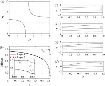
. In figure 4(a) we plot the numerical value of
 $K$
as a function of
 $\mathscr{A}_{1}$
for
 $\mathscr{C}_{1}=\mathscr{C}_{2}=1$
. We note that in some parameter regions the value of
 $K$
can be negative, in which case the uniform base state is unstable for all
 $\mathscr{A}_{3}\geqslant 0$
.
Development of a perturbation of the form (3.10) with fixed wavenumber
 $k={\rm\pi}$
,
 $\mathscr{C}_{1}=\mathscr{C}_{2}=1$
,
 $\tilde{{\it\mu}}=2$
,
 $h_{c1}=0$
,
 $h_{c2}=0.1$
,
 ${\it\delta}=0.01$
, with
 $h_{2}^{\prime }$
determined by (4.5): (a)
 $K$
as defined by (4.7); (b) temporal evolution of the minimum thickness in both layers with
 $\mathscr{A}_{1}=0$
and
 $\mathscr{A}_{3}=10$
for a surfactant-laden system with large viscosity contrast, governed by (4.4); the inset shows a close-up of the approach to rupture; (c–f) snapshots of the two films at various times illustrating evolution towards isolated dewetting ((c)
 $t=0.500$
; (d)
 $t=0.605$
; (e)
 $t=0.615$
; (f)
 $t=0.622$
).

4.1.3. Nonlinear dewetting
In contrast to the surfactant-free configuration, in addition to varicose disturbances the system (4.4) also admits sinuous solutions, which may provide a potential mechanism for isolated rupture. To explore this possibility we must analyse the full nonlinear equations (4.4), which exhibit an identical structure to (3.3), and so we employ an identical numerical method to solve this system. We prescribe an initial condition of the form (3.10). To prevent rupture and facilitate dewetting and retraction of the liquid layers we use a modified van der Waals pressure with a cutoff at a finite thickness
 $h_{cj}$
(a cojoining–disjoining pressure), where (2.9) is modified to
 $$\begin{eqnarray}\breve{{\it\phi}}_{1}={\it\phi}_{1}-\frac{\mathscr{A}_{1}h_{c1}^{3}}{h_{1}^{m}},\quad \breve{{\it\phi}}_{2}={\it\phi}_{2}-\frac{\mathscr{A}_{3}h_{c2}^{3}}{h_{2}^{m}}.\end{eqnarray}$$
This form of the cutoff term in the van der Waals pressure has an algebraic dependence on the layer thickness
 $h_{j}~(j=1,2)$
, where the exponent
 $m$
must be chosen to be greater than 3; this assumption has been used widely for various values of
 $m$
(Schwartz et al.
Reference Schwartz, Roy, Eley and Petrash2001; Seemann, Herminghaus & Jacobs Reference Seemann, Herminghaus and Jacobs2001). In this study we fix
 $m=6$
, but the precise value of
 $m$
does not influence the dynamics of rupture significantly. Other physically motivated forms of the cutoff in the van der Waals pressure have been used elsewhere, such as an exponential decay in the layer thickness (Pototsky et al.
Reference Pototsky, Bestehorn, Merkt and Thiele2004).
The canonical rupture behaviour when viewed via the temporal contraction of the film is similar to that for a surfactant-free bi-layer, with the film rupturing in finite time (figure 4
b). However, the bi-layer film thickness profiles now reveal an entirely different rupture mechanism whereby layer 2 thins with time through excitation of the initial perturbation, during which layer 1 remains of order-one thickness (figure 4
c–f). Once layer 2 becomes sufficiently thin the cutoff term in the van der Waals potential (4.8) becomes important (
 $h_{c2}>0$
) and a film of constant thickness is extruded in layer 2 (figure 4
f). Unlike in the surfactant-free case, we now observe a deformation in the centreline between the two fluids. Such behaviour is indicative of a separated rupture, as observed in the experiments when surfactant is adsorbed at the water–air interface. We refer to such dynamics as dewetting.
Although we posed a sinuous initial perturbation (as it emerges for this case that
 $h_{2}^{\prime }<0$
), in which layer 1 is bulged and layer 2 is contracted at
 $x=0$
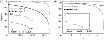
, which lends itself to promoting isolated rupture in layer 2, we find that even when the initial condition is varicose the system still exhibits isolated-rupture behaviour, as illustrated in figure 5(a). Thus, the separated rupture is not simply an artefact of a fortuitous choice of initial perturbation. Furthermore, the isolated rupture is not restricted to a carefully chosen van der Waals force configuration and is observed even when the van der Waals forces in both layers are comparable, as illustrated in figure 5(b), where in this case the isolated rupture is observed in layer 1.
Nonlinear simulations of free-film rupture for a surfactant-laden layer 1 with a large viscosity contrast, governed by (4.4), with
 $\mathscr{C}_{1}=\mathscr{C}_{2}=1$
,
 $\tilde{{\it\mu}}=2$
,
 $h_{c1}=h_{c2}=0.1$
and
 ${\it\delta}=0.01$
for (a) an initially varicose perturbation with
 $\mathscr{A}_{1}=0$
and
 $\mathscr{A}_{3}=25$
, and (b) a case where van der Waals attractions act in both layers simultaneously with
 $\mathscr{A}_{1}=\mathscr{A}_{3}=2$
.

4.2. Case 2: order-one viscosity contrast
4.2.1. Governing equations
In the limit when
 $\overline{{\it\mu}}=O(1)$
the leading-order governing equations become
 $$\begin{eqnarray}\displaystyle & \boldsymbol{{\rm\nabla}}\boldsymbol{\cdot }\boldsymbol{u}_{1}=0,\quad \tilde{p}_{1,x}+{\it\phi}_{1,x}=u_{1,yy},\quad \tilde{p}_{1,y}+{\it\phi}_{1,y}=0,\quad H-h_{1}<y<H, & \displaystyle\end{eqnarray}$$
 $$\begin{eqnarray}\displaystyle & \boldsymbol{{\rm\nabla}}\boldsymbol{\cdot }\boldsymbol{u}_{2}=0,\quad \tilde{p}_{2,x}+{\it\phi}_{2,x}=\overline{{\it\mu}}u_{2,yy},\quad \tilde{p}_{2,y}+{\it\phi}_{2,y}=0,\quad H<y<H+h_{2}. & \displaystyle\end{eqnarray}$$
The leading-order boundary conditions are
 $$\begin{eqnarray}\displaystyle & v_{1}=(H-h_{1})_{t},\quad u_{1}=0,\quad -\tilde{p}_{1}=-\mathscr{C}_{1}(H-h_{1})_{xx}, & \displaystyle\end{eqnarray}$$
on
 $y=H-h_{1}$
,
 $$\begin{eqnarray}\displaystyle & u_{1}=u_{2},\quad v_{1}=v_{2}=H_{t}+u_{1}H_{x},\quad \overline{{\it\mu}}u_{2,y}=u_{1,y},\quad -\tilde{p}_{2}+\tilde{p}_{1}=-H_{xx}, & \displaystyle\end{eqnarray}$$
on
 $y=H$
and
 $$\begin{eqnarray}\displaystyle & v_{2}=(H+h_{2})_{t}+u_{2}(H+h_{2})_{x},\quad u_{2,y}=0,\quad -\tilde{p}_{2}=\mathscr{C}_{2}(H+h_{2})_{xx}, & \displaystyle\end{eqnarray}$$
on
 $y=H+h_{2}$
.
Since
 $\tilde{p}_{1}$
and
 $\tilde{p}_{2}$
are independent of
 $y$
, the
 $x$
-momentum equations in (4.9a,b
) can be integrated to construct the velocity profile across both layers. Combining with the continuity and kinematic conditions, the leading-order governing equations for the thicknesses of both layers are then given by
 $$\begin{eqnarray}\displaystyle & \displaystyle h_{1,t}-\left(\frac{h_{1}^{3}}{3}\overline{p}_{1,x}+\frac{h_{1}^{2}h_{2}}{2\overline{{\it\mu}}}\overline{p}_{2,x}\right)_{x}=0, & \displaystyle\end{eqnarray}$$
 $$\begin{eqnarray}\displaystyle & \displaystyle h_{2,t}-\left(\frac{h_{2}^{3}}{3\overline{{\it\mu}}}\overline{p}_{2,x}+\frac{h_{1}h_{2}^{2}}{\overline{{\it\mu}}}\overline{p}_{2,x}+\frac{h_{1}^{2}h_{2}}{2}\overline{p}_{1,x}\right)_{x}=0, & \displaystyle\end{eqnarray}$$
 $\overline{p}_{j}~(j=1,2)$
is again given by (3.4). As before, the shape of the bi-layer midline is given by (3.5). It is interesting to note that these governing equations for a bi-layer free film with order-one viscosity contrast and a surfactant-laden interface are equivalent to those derived by Pototsky et al. (Reference Pototsky, Bestehorn, Merkt and Thiele2004) (although their system was expressed in variational form) for a bi-layer film on a rigid substrate. Their analysis focused on the final static profile of the bi-layer system, but we instead focus on the dynamics, the order of rupture and dewetting, and examine the conditions required for a separated rupture event.
4.2.2. Linear stability analysis
The stability properties of this system are qualitatively similar to those reported in § 4.1.2, and an extensive stability analysis of this system was reported by Pototsky et al. (Reference Pototsky, Bestehorn, Merkt and Thiele2004) for a bi-layer thin film on a rigid substrate. The dispersion relation is of the form
 $$\begin{eqnarray}\displaystyle & d{\it\omega}^{2}+e{\it\omega}+f=0, & \displaystyle\end{eqnarray}$$
where
 $$\begin{eqnarray}\displaystyle d & = & \displaystyle 36\overline{{\it\mu}}(1+\mathscr{C}_{1}+\mathscr{C}_{2})\overline{h}_{2}^{2},\end{eqnarray}$$
 $$\begin{eqnarray}\displaystyle e & = & \displaystyle -36(1+\mathscr{C}_{1}+\mathscr{C}_{2})(\mathscr{A}_{3}(3+\overline{h}_{2})+\mathscr{A}_{1}\overline{{\it\mu}}\overline{h}_{2}^{2})k^{2}+6\overline{h}_{2}^{2}\nonumber\\ \displaystyle & & \displaystyle \times \,(2\overline{{\it\mu}}\mathscr{C}_{1}(1+\mathscr{C}_{2})+3(1+\overline{{\it\mu}})\mathscr{C}_{1}\mathscr{C}_{2}\overline{h}_{2}+6(1+\mathscr{C}_{1})\mathscr{C}_{2}\overline{h}_{2}^{2}+2\mathscr{C}_{2}(1+\mathscr{C}_{1})\overline{h}_{2}^{3})k^{4},\nonumber\\ \displaystyle & & \displaystyle\end{eqnarray}$$
 $$\begin{eqnarray}\displaystyle f & = & \displaystyle 9\mathscr{A}_{1}\mathscr{A}_{3}(1+\mathscr{C}_{1}+\mathscr{C}_{2})(3+4\overline{h}_{2})k^{4}+\mathscr{C}_{1}\mathscr{C}_{2}\overline{h}_{2}^{4}(3+4\overline{h}_{2})k^{8}\nonumber\\ \displaystyle & & \displaystyle -\,3(3+4\overline{h}_{2})(\mathscr{A}_{3}\mathscr{C}_{1}(1+\mathscr{C}_{2})+\mathscr{A}_{1}(1+\mathscr{C}_{1})\mathscr{C}_{2}\overline{h}_{2}^{4})k^{6}.\end{eqnarray}$$
For these equations, the discriminant now can be negative, which reveals the possibility for travelling waves through complex growth rates, illustrated in shaded regions in the phase space spanned by
 $k$
and
 $\mathscr{A}_{1}$
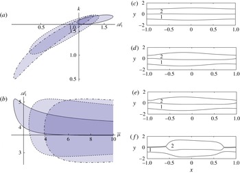
in figure 6(a); travelling-wave solutions were also found by Fisher & Golovin (Reference Fisher and Golovin2007) using a weakly nonlinear model. As
 $\overline{{\it\mu}}$
increases the region in which travelling-wave solutions exist becomes longer and thinner, becoming infinitely thin as
 $\overline{{\it\mu}}\rightarrow \infty$
(figure 6
a), indicating why travelling-wave behaviour was not observed in § 4.2. Again fixing the perturbation wavenumber
 $k={\rm\pi}$
the corresponding regions of the phase space that exhibit travelling rupture are shown in figure 6(b).
Travelling-wave solutions in a surfactant-laden layer 1 with an order-one viscosity contrast, governed by (4.11a
), with
 $\overline{h}_{2}=\mathscr{C}_{1}=\mathscr{C}_{2}=1$
. The shaded area highlights the region in which travelling-wave solutions exist, in (a)
 $k{-}\mathscr{A}_{1}$
phase space with
 $\overline{{\it\mu}}=2$
(solid), 10 (dashed) and 50 (dot-dashed); (b)
 $\mathscr{A}_{1}{-}\overline{{\it\mu}}$
phase space with
 $\mathscr{A}_{2}=3$
(solid), 4 (dashed) and 5 (dot-dashed) for
 $k={\rm\pi}$
; (c–f) snapshots of the surfactant-laden system with order-one viscosity contrast (4.10) at various times, illustrating the transverse propagation of the rupture position for an initial perturbation of the form (3.10) with fixed wavenumber
 $k={\rm\pi}$
,
 $\mathscr{C}_{1}=\mathscr{C}_{2}=\overline{{\it\mu}}=1$
,
 $h_{c1}=0$
,
 $h_{c2}=0.1$
,
 ${\it\delta}=0.01$
((c)
 $t=2.000$
; (d)
 $t=2.285$
; (e)
 $t=2.290$
; (f)
 $t=2.295$
).

4.2.3. Nonlinear dewetting
The system (4.10) consists of two coupled parabolic PDEs, but since this system admits travelling instabilities we cannot, in general, assume symmetry of solutions about
 $x=0$
. Instead we solve the governing equations (4.10) on a periodic domain
 $-1\leqslant x\leqslant 1$
using a semi-implicit time-stepping method that is first order in time, where spatial derivatives are discretized using fourth-order centred finite differences (similar to the method used by Stewart, Waters & Jensen Reference Stewart, Waters and Jensen2009). To prevent finite-time rupture we again use a modified van der Waals pressure with a cutoff at a finite thickness as described by (4.8). Interface shapes at four different times from a typical nonlinear simulation of travelling rupture are shown in figure 6(c–f). Similarly to the results for large viscosity contrast between the layers (§ 4.1) we observe the combined thinning of layer 2 through an instability propagating to the right across the domain, while layer 1 deforms but remains of order-one thickness (figure 6
c–f). As the instability grows, eventually layer 2 becomes sufficiently thin to trigger the cutoff term in the van der Waals pressure, depositing a thin precursor film of constant thickness
 $h_{c2}$
as layer 2 retracts across layer 1 (figure 6
f) in a similar manner to § 4.1.3.
5. Experimental insight
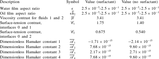
Having explored a general model for the stability of a bi-layer free liquid film, we now use this model to provide a better understanding of the experimental observations of Feng et al. (Reference Feng, Roché, Vigolo, Arnaudov, Stoyanov, Gurkov, Tsutsumanova and Stone2014). Taking hexadecane as a typical alkane, values for the experimental parameters are listed in table 1 both for no surfactant and for an abundance of
 $\text{C}_{12}\text{TAB}$
surfactant. The four-dimensional Hamaker constants have been estimated using the method outlined by Pototsky et al. (Reference Pototsky, Bestehorn, Merkt and Thiele2005) based on the long-range interaction energy constructed by Israelachvili (Reference Israelachvili2011) for a pair of parallel interfaces. We use typical values for the refractive indices of the three media (air, water, alkane) and, following Pototsky et al. (Reference Pototsky, Bestehorn, Merkt and Thiele2005), we assume that the absorption frequencies of all three media are equal (
 ${\it\nu}_{e}\approx 3\times 10^{15}~\text{Hz}$
) and neglect the zero-frequency contribution.
Typical experimental parameter values for the bi-layer system of hexadecane and an aqueous surfactant solution (
 $[\text{C}_{12}\text{TAB}]=1.4~\text{mM}$
) (Matsubara et al.
Reference Matsubara, Ikeda, Takiue, Aratono and Bain2003).

We observe that the dimensional Hamaker constant
 $A_{1}$
is negative, so the van der Waals force between the air–water and oil–water interfaces is repulsive across layer 1. In §§ 3 and 4 we assumed that the Hamaker constants were non-negative (attractive van der Waals forces), so we now investigate the influence of repulsive van der Waals forces on the rupture mechanics.
The dimensionless Hamaker constants defined in (2.7a
) depend on the aspect ratio of the aqueous film
 ${\it\epsilon}$
; we wish to determine how
 ${\it\epsilon}$
influences the rupture behaviour, and so we rewrite the dimensionless Hamaker constants in the form
 $$\begin{eqnarray}\mathscr{A}_{n}=\frac{1}{{\it\epsilon}^{4}}\overline{\mathscr{A}}_{n}\quad (n=1,\dots ,4),\end{eqnarray}$$
where the rescaled Hamaker constants
 $\overline{\mathscr{A}}_{n}~(n=1,\dots ,4)$
can be determined directly from the values reported in table 1. Typical values for the dimensionless groups are given in table 2.
Dimensionless parameters in the model estimated from the experimental parameters in table 1.

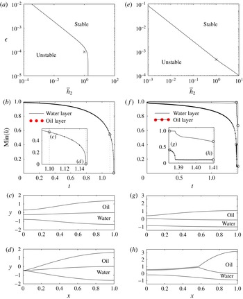
Rupture and dewetting of a bi-layer free film for the parameter values listed in table 1 corresponding to the experiments of Feng et al. (Reference Feng, Roché, Vigolo, Arnaudov, Stoyanov, Gurkov, Tsutsumanova and Stone2014). (a–d) No surfactant on the air–aqueous interface, satisfying (3.3): (a) stability of the uniform state in the parameter space spanned by the aspect ratio of the aqueous layer,
 ${\it\epsilon}$
, and the thickness contrast between the layers
 $\overline{h}_{2}$
; (b) minimal thicknesses of both layers at the point marked by a cross in (a), where the inset shows a close-up of behaviour close to rupture; simulations are initiated using (3.6) with
 $h_{2}^{\prime }=1$
,
 $U^{\prime }=0$
and
 ${\it\delta}=0.01$
; (c,d) typical results showing simultaneous rupture of both layers ((c)
 $t=1.100$
; (d)
 $t=1.149$
). (e–h) Abundance of surfactant on the air–aqueous interface, satisfying (4.10) for an order-one viscosity contrast (as in § 4.2): (e) stability of the uniform state in the parameter space spanned by
 ${\it\epsilon}$
and
 $\overline{h}_{2}$
; (f) minimal thickness of both layers at the point marked by a cross in (e), where the inset shows a close-up of behaviour close to dewetting of layer 2; simulations are initiated using (3.6) with
 $h_{2}^{\prime }=1$
and
 ${\it\delta}=0.01$
; (g,h) typical stills of an isolated rupture of the oil layer and subsequent dewetting across the water layer ((g)
 $t=1.385$
; (h)
 $t=1.410$
).

For the experimental parameters in the absence of surfactant, we explore the linear stability of the uniform state in the space spanned by the dimensionless thickness of layer 1,
 ${\it\epsilon}$
, and the thickness contrast between the two layers,
 $\overline{h}_{2}$
, in figure 7(a); the uniform base state is unstable to the left of the curve. For these parameters we observe that the bi-layer system is always stable when the thickness contrast between the two layers exceeds a threshold
 $\overline{h}_{2}\gtrsim 1.758$
. Setting
 ${\it\epsilon}=10^{-4}$
and
 $\overline{h}_{2}=1$
(the point marked with a cross in the unstable region in figure 7
a) we solve (3.3) numerically using the method outlined in § 3.3; the corresponding minimal film thickness in both layers is illustrated in figure 7(b), while typical profiles of the film are shown in figure 7(c,d). This example demonstrates rupture of both layers simultaneously, as predicted in § 3.1 for the model parameters.
Similarly, for experimental parameters with an abundance of surfactant we consider an
 $O(1)$
viscosity contrast between the layers described by (4.10) in § 4.2. We again explore the linear stability of the uniform state in the space spanned by
 ${\it\epsilon}$
and
 $\overline{h}_{2}$
, as shown in figure 7(e), where the basic state is unstable to the left of the curve. In contrast to figure 6(a), we now find that this bi-layer system is always unstable for any
 $\overline{h}_{2}$
provided that
 ${\it\epsilon}$
is chosen sufficiently small. For example, setting
 ${\it\epsilon}=2\times 10^{-4}$
and
 $\overline{h}_{2}=1$
(the point marked with a cross in the unstable region in 7
e) we present nonlinear solutions of (4.10) obtained numerically using the semi-implicit time-stepping method discussed in § 4.2.3; the corresponding minimal film thickness in both layers is illustrated in figure 7(f), while typical profiles of the film are shown in figure 7(g,h). This example demonstrates an isolated rupture of the oil layer only (figure 7
g), at which point it then retracts across the aqueous layer depositing a precursor film (figure 7
h), consistent with the behaviour illustrated in § 4 for the model parameters.
6. Discussion
We have considered the stability of a large-aspect-ratio bi-layer free film formed by two immiscible liquid layers to van der Waals intermolecular attractions. This provides a simple set-up that captures many of the features present in the formation of two films as a bubble of air approaches the free surface of a water bath coated with a thin layer of oil. Here, the experiments of Feng et al. (Reference Feng, Roché, Vigolo, Arnaudov, Stoyanov, Gurkov, Tsutsumanova and Stone2014) showed that, in the presence of surfactant in the water phase, the system exhibits a distinct rupture and dewetting of the oil layer followed by rupture of the water layer, which can be up to several hundreds of milliseconds later. However, later experiments by the same authors have shown that in the absence of surfactant both the oil layer and the water separating the bubble from the surrounding air rupture simultaneously as the bubble penetrates the surface in almost all cases. In agreement with these experiments, we have demonstrated that the presence of surfactant on the air–water interface holds the key to observing a separated rupture event.
In the absence of surfactant, the gas–liquid interfaces are free of tangential stress, so that when the liquid layers are sufficiently thin attractive forces between the interfaces drive both the oil and water layers to thin simultaneously: distinct rupture of one layer is impossible. We have shown that this behaviour is universally true, with rupture taking place in both fluids even when the van der Waals attractive force is only acting in one layer (figure 3). However, when the air–water interface is tangentially immobile, mimicking an abundance of surfactant, the thinning of one layer is able to induce thickening in the other, so that isolated rupture and dewetting of one layer only is observed (figure 4). In addition, when viscous shear is present at leading order in both layers simultaneously, a linear stability analysis uncovered the possibility of travelling-wave instabilities in a small parameter window (figure 6 a,b) similar to those predicted by Fisher & Golovin (Reference Fisher and Golovin2007) for films on a solid substrate, which we verified by a full nonlinear simulation (figure 6 c–f). However, in no cases did we observe a transition to a fully nonlinear travelling wave and subsequent suppression of rupture due to shear (as reported in similar systems by Davis, Gratton & Davis (Reference Davis, Gratton and Davis2010) and Kalpathy, Francis & Kumar (Reference Kalpathy, Francis and Kumar2010)).
The distinction between the simultaneous and separated rupture triggered by surfactant on the air–aqueous interface is also evident using parameter values relevant to the experiments of Feng et al. (Reference Feng, Roché, Vigolo, Arnaudov, Stoyanov, Gurkov, Tsutsumanova and Stone2014) (figure 7). When the oil and water layers are of equal initial thickness, for a film of length 4 mm both regimes predict a comparable critical film thickness of 608 nm (809 nm) for a surfactant-free (surfactant-laden) system. The surfactant-laden system is always unstable when the water layer becomes sufficiently thin (figure 7 e), but in the surfactant-free case the uniform initial state is always stable when the thickness of the oil layer exceeds that of the water layer by a factor of approximately 1.75 (figure 7 a).
Since bubbles are easily generated in nature, such a bi-layer system may be observed when a bubble floats on the ocean surface. As a result, some of the features highlighted by our model, such as the role of the surfactant effects and the thickness of the oil layer, might be used to identify some control parameters that influence the rupture behaviour in more complex real-life scenarios, such as understanding the behaviour of oil slicks floating at sea.
The model presented herein is a deliberately simplified representation of the experimental set-up, ignoring the large-scale curvature of the bi-layer midline and the thinning of both layers driven by both elongation of the film and drainage due to capillary viscous suction into the adjacent Plateau borders (Howell Reference Howell1999; Anderson et al. Reference Anderson, Brush and Davis2010). In addition, we have neglected the dynamics of the surfactant adsorption and desorption onto the water–air and water–oil interfaces, restricting its influence to the boundary condition on the air–water interface. Despite these limitations, the model corroborates the experimental observations of Feng et al. (Reference Feng, Roché, Vigolo, Arnaudov, Stoyanov, Gurkov, Tsutsumanova and Stone2014) and is able to provide parametric regimes in which we expect to observe distinct rupture behaviour, with regard to wettability expressed through the relative strengths of the van der Waals forces, and regimes in which simultaneous rupture is unavoidable. Such predictions should ultimately lead to greater control in manipulating multilayer free-film systems.
Acknowledgements
The authors would like to thank the Oxford Princeton Collaborative Workshop participants for useful discussions (January 2013, January 2014). J.F. and H.A.S. thank Unilever Research and the CMEDS grant from BP/The Gulf of Mexico Research Initiative.