1. Introduction

Suppose that you had your temperature taken and that the thermometer correctly indicated a healthy temperature of 37°C (or 98.6°F). What would have happened had the thermometer been broken so that its reading was exactly .5°C higher? Would your body temperature have been different from what it actually was? Would you have subsequently taken a pill to reduce your fever?

Inspired by Stalnaker (Reference Stalnaker and Cornman1968) and Lewis (Reference Lewis1973), most philosophers think that the answers to these questions can be determined by checking whether the closest possible world(s) in which the thermometer is broken is/are world(s) in which your body temperature is different or is/are world(s) in which you take the pill. What does this closeness consist in? Most philosophers treat worlds as close to the actual world to the extent that they are similar to the actual world, where what counts as similar varies with context. Although the question of what settles the degree of similarity between possible worlds remains controversial, it is standardly thought that the similarity relation must capture the way in which counterfactual dependence typically tracks causal dependence. For example, given our knowledge of the way in which thermometers work, and of how people respond when thermometers register slight fevers, the relevant notion of similarity should vindicate the claim that the closest possible worlds in which the thermometer is broken may be worlds in which you subsequently take a pill (since the thermometer’s appearance has a causal effect on whether you take the pill) but may not be worlds in which your body temperature is different from what it actually is (since your body temperature is causally upstream from the thermometer’s appearance).

Lewis (Reference Lewis1979) famously used a complicated system of weights and priorities to develop an account of ‘similarity’ that delivers these results, but many philosophers (e.g., Hausman Reference Hausman1998; Woodward Reference Woodward2005) have convincingly argued that Lewis’s account is inadequate for several reasons, chief among which is its inability to rigorously establish definite similarity orderings.Footnote ¹ Meanwhile, some other authors (e.g., Woodward Reference Woodward2005; Pearl Reference Pearl2009; Briggs Reference Briggs2012; Halpern Reference Halpern2016) have argued that graphical causal models can be used to develop a more precise account that does at least as well at capturing our intuitions about counterfactual dependence. We agree with these authors. Although the details of these accounts vary from one author to the next, we are impressed with their general ability to capture counterfactual reasoning in a rigorous way.

There is, however, at least one important limitation to these authors’ accounts. They say nothing about what would obtain were the causal structure to be different from what it actually is or from what we believe it to be. The basic issue is that a graphical causal model specifies how the worlds that the causal model describes are more and less similar to each other, but it says nothing about how the causal model itself is more or less similar to other causal models. Thus, these accounts are silent, for example, with respect to how we should update our beliefs under the counterfactual supposition that your body temperature causally depends on the thermometer’s appearance (rather than the other way around). Should we still believe that whether you take a pill is causally downstream from your body temperature? If you want an answer to this question, then you must look elsewhere.

In this article, we explore the possibility of using graphical causal models to resolve counterfactual queries about causal structure by introducing a notion of similarity between causal graphs. Specifically, we aim to answer queries like the above by determining whether the counterfactual graph that is most similar to the original graph is one in which taking a pill is causally downstream from your body temperature. Since the causal structure of the world may be immutable, and since we seldom, if ever, are in a position to manipulate the causal structure of the world, it may seem that this project is valuable only insofar as it informs science fiction or insofar as it quenches our natural thirst for knowledge about how things would be different were the world to be causally different. (After all, the primary reason that we value knowing what would happen were the thermometer to report inaccurately is that thermometers sometimes do break, and we care about the very real consequences of their breaking.) We must admit that some of our interest in these counterfactual queries is driven by curiosity, but more pragmatic readers need not worry. We are also driven by our desire to make progress on the practically important problem of how agents should update their standing beliefs about causal structure when they learn that they are incorrect.

It is clear from work at the intersection of psychology, epistemology, and artificial intelligence that intelligent creatures like us often use qualitative beliefs about causal structure to organize our quantitative beliefs about evidential and counterfactual (ir)relevance.Footnote ² When our beliefs about causal structure play this role, we do not entertain alternate possible causal structures; rather, we take a particular causal structure as given and let it guide our evidential and practical reasoning. In so doing, we open ourselves up to the possibility of learning something that conflicts with our standing qualitative beliefs (e.g., when we initially believe that X causes Y and subsequently learn that Y temporally precedes X), and we need a method of belief revision that is well suited to this kind of learning.Footnote ³ In this setting, we submit that the agent should replace her belief in the original causal graph with a belief in a new causal graph that is among the graphs most similar to the original that are compatible with the new evidence.

Consider our attitudes toward the healthiness of foods. In order to make the world easier to navigate, we often reason as though we are certain that a particular food does (or does not) causally promote heart disease. (This considerably simplifies our deliberation about whether to eat the relevant food.) But when we learn later that we are wrong (e.g., because our best science now tells us that red meat consumption does causally promote heart disease), we need to know what causal structure to accept. Our proposal is that we should accept whatever graph is closest to our prior causal graph among the set of graphs that include the learned causal relationship between red meat consumption and heart disease.

In order to develop a treatment of similarity that is up to the task at hand, we need to think carefully about what information is contained within a causal graph. We will see in what follows that causal graphs are used to represent how an agent’s beliefs about causal structure constrain her beliefs about evidential relevance and counterfactual relevance and that these two kinds of constraints operate somewhat independently from each other. To address both considerations, we introduce an evidential similarity relation in section 2 and a counterfactual similarity relation in section 3 and then consider possible ways of incorporating both kinds of similarity into one master concept in section 4. We abstain from arguing for any particular master concept of similarity because it seems that there may be some contexts in which one master concept is appropriately deployed and others in which another is appropriately deployed. But in section 5, we do take stock of when it matters which concept we use, that is, of when (and when not) counterfactual queries about causal structure have the same answers regardless of which potential master concept is deployed. We argue that the answers to these counterfactual queries may stand on firmer ground than others because, unlike others, they do not depend on whether we give more priority to evidential similarity or counterfactual similarity.

2. Evidential Similarity

In order to say what accounts for the similarity between causal graphs, we need to first take stock of what information is contained within a causal graph. Our first task is thus to identify the basic properties that distinguish causal structures.

Given some set of variables, V, we define a causal structure over V as a directed acyclic graph (DAG) over V, that is, a set of directed edges (or arrows) over V that are arranged such that no directed path forms a cycle, where the directed edges are taken to represent direct causal dependencies. For example, if H represents height, D represents diet, and I represents intelligence, then the DAG in figure 1 represents the causal structure according to which diet has a direct causal influence on intelligence, and no other (direct or indirect) causal relationships obtain between the variables in V.

Figure 1.

Directed acyclic graph.

One way of capturing the characteristic content of this particular causal structure is that it has substantial implications for the evidential relationships between H, D, and I. For example, if this really is the true causal structure (and if we have not omitted any common causes), then H and D should be probabilistically independent. This is because there should be no correlation between the respective values of two variables when there is absolutely no causal relationship between them.

The most powerful and widely accepted way of cataloging the evidential implications of a causal structure is given by the causal Markov condition (CMC), a generalization of Reichenbach’s common cause principle. The CMC provides a general procedure for inferring probabilistic independencies (such as the independence between height and diet) from DAGs and also helps us narrow down the set of DAGs that are compatible with a given probability distribution.Footnote ⁴

One important aspect of the CMC is that it sometimes treats distinct DAGs as compatible with the same probability distributions. To illustrate, consider the causal structures, G and G*, that are depicted in figure 2. According to the CMC, G and G* both imply that H is probabilistically independent of both D and I, and they allow for the possibility that D is correlated with I. But according to the CMC, the direction of the causal dependence between D and I makes no difference with respect to the probability distribution. Structures like G and G* (i.e., structures that imply the same probabilistic independencies) are known as Markov equivalent.

Figure 2.

Markov equivalence.

If we hope to explicate the notion of similarity between causal graphs in a way that tracks their role in evidential reasoning, it seems that there should be some dimension of similarity according to which two Markov equivalent graphs are always classified as maximally similar. More generally, a natural approach to assessing the similarity between distinct causal structures is to measure the extent to which they have the same implications regarding the evidential relationships that obtain among the given variables. This motivates the following definition:

Definition 1. Fix a variable set V and let N_P denote the cardinality of the set of all possible conditional independencies that can hold among the variables in V. Given a causal structure G, let P_G denote the set of conditional independencies entailed by G and the CMC. Then we define the ‘evidential distance’ between two causal structures G and G* over V to be

$d_E\left(G,G^{*}\right)=\frac{\left|P_G\Delta P_{G^{*}}\right|}{N_P},$

where Δ is the symmetric difference.

The evidential distance between G and G*, or d_E(G, G*), simply counts the number of conditional independencies that are entailed by one but not both of G and G*, normalized by the total number of possible conditional independencies that could hold between the variables in V.Footnote ⁵

Intuitively, d_E(G, G*) can be thought of as encoding the extent to which G and G* disagree regarding the evidential relationships between the variables in V. For example, it will be zero if and only if G and G* are Markov equivalent. To further illustrate, consider the basic structures

$\begin{array}{}& G_1:X\to Y\to Z,G_2:X\leftarrow Y\to Z,G_3:X\to Y\leftarrow Z\mathrm{.}\end{array}$

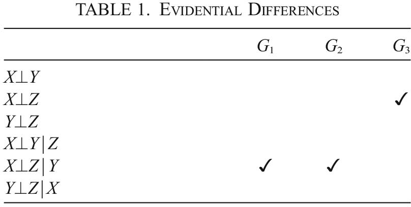
To calculate the evidential distance between them, we simply count how many probabilistic conditional independencies they disagree on and divide by the total number of possible conditional independencies, as in table 1.Footnote ⁶

Table 1.

Evidential Differences

This yields the result that $d_E\left(G_1,G_2\right)=0$ (as expected, since G ₁ and G ₂ are Markov equivalent), and $d_E\left(G_1,G_3\right)=1/3=d_E\left(G_2,G_3\right)$ since both G ₁ and G ₂ disagree with G ₃ about two of the six possible independencies.

3. Counterfactual Similarity

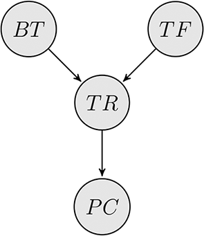
Of course, the characteristic content of a causal structure is not exhausted by its evidential implications. It is widely acknowledged that causal structure also plays a crucial role both in assessing the veracity of counterfactuals and in predicting the outcomes of prospective interventions. To illustrate, let BT represent body temperature, TF represent whether the thermometer properly functions, TR represent the thermometer reading, and PC represent whether a fever-reducing pill is subsequently consumed. The intuitive causal structure in this case is depicted in figure 3.

Figure 3.

Thermometer.

As we mentioned in the introduction, this DAG gives us a good handle on what counterfactually depends on what in most contexts. For example, we know that both TR and PC counterfactually depend on BT but that TF does not counterfactually depend on BT. Similarly, as mentioned before, we know that BT and TF do not counterfactually depend on TR, and PC plausibly does counterfactually depend on TR.

In the interventionist framework, there are two simple ways to account for these dependencies. First, the CMC entails that the intervention on X can be associated only with variables that are causally downstream from X, and counterfactual supposition plausibly corresponds to the supposition that one intervenes to set X to x.Footnote ⁷ Second, we can think of a DAG as imposing a partial counterfactual ordering on V, where Y comes directly after X in the ordering exactly when X is a direct cause of Y and where Y possibly counterfactually depends on X exactly when Y (directly or indirectly) follows X in the partial ordering.Footnote ⁸ Thus, this graph imposes a counterfactual ordering according to which BT and TF directly precede TR, BT and TF are not ordered, and PC directly follows TR and indirectly follows both BT and TF.

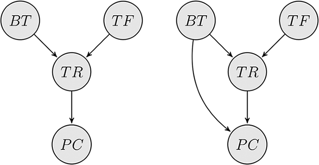
We see now that DAGs not only have implications with respect to the evidential relationships that obtain between the variables in V but also imply constraints on the possible counterfactual dependencies that hold between those variables. Just as two distinct DAGs can embody the same evidential implications (e.g., when they are Markov equivalent), two distinct DAGs can embody the same counterfactual implications. To illustrate, consider the two causal structures that appear in figure 4. Call the structure on the left G and the structure on the right G*. Structure G* is identical to G except for the fact that it includes an additional direct causal influence from BT to PC. This additional causal relationship does not allow any new counterfactual dependencies, since PC already indirectly follows BT in the counterfactual ordering implied by G. Thus, G and G* encode exactly the same sets of possible counterfactual dependencies, and we can call them counterfactually equivalent.Footnote ⁹

Figure 4.

Counterfactual equivalence.

In section 2 we presented a method for evaluating the degree to which different causal structures G and G* have the same evidential implications. An analogous method can be defined for evaluating the degree to which G and G* are counterfactually similar. Just as we required that, from the evidential perspective, Markov equivalent DAGs should be maximally similar, we require that counterfactually equivalent DAGs should be maximally similar from the counterfactual perspective.

Definition 2. Fix a variable set V and let N_C denote the cardinality of the set of all possible counterfactual dependencies that can hold among the variables in V. Given a causal structure G, let C_G denote the set of possible counterfactual dependencies allowed by G and the CMC. Then we define the ‘counterfactual distance’ between two causal structures G and G* over V to be

$d_C\left(G,G^{*}\right)=\frac{\left|C_G\Delta C_{G^{*}}\right|}{N_C}\mathrm{.}$

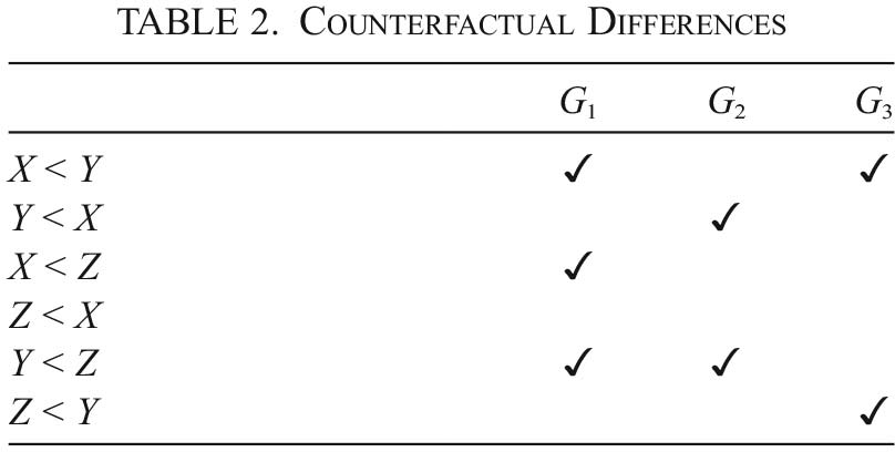
Given two causal structures G and G* over V, d_C(G, G*) simply counts all those possible counterfactual dependencies about which G and G* disagree and normalizes by the cardinality of the set of possible counterfactual dependencies among V. It immediately follows that $d_C\left(G,G^{*}\right)=0$ if and only if G and G* are counterfactually equivalent. To illustrate how d_C measures the distance between causal structures and its relationship to d_E, recall the basic structures G ₁, G ₂, G ₃ from the previous section. Table 2 shows how we calculate the counterfactual distance between these structures (where $X<Y$ means that Y possibly counterfactually depends on X).

Table 2.

Counterfactual Differences

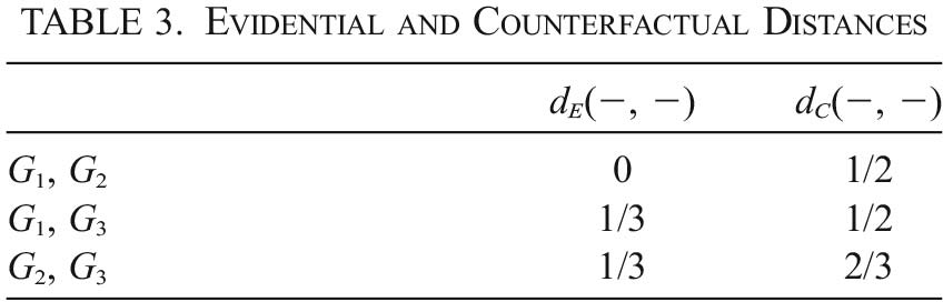
The evidential and counterfactual distances between these structures is summarized in table 3. This table helps us to see how evidential distance and counterfactual distance can come apart. For example, G ₂ and G ₃ are equally counterfactually close to G ₁, but when it comes to evidential distance, G ₂ is closer to G ₁ than G ₃ is close to G ₁. Because these two metrics are independent in this way, if we settle counterfactual queries by minimizing evidential distance, we will not always arrive at the DAG (or set of DAGs) that minimizes counterfactual distance. Likewise, if we minimize counterfactual distance, we will not always arrive at the DAG (or set of DAGs) that minimizes evidential distance. For example, if we start off believing $X\to Y\to Z$ and then learn that, as a matter of fact, $Y\to X$ , it is easy to see that the evidentially closest DAG is $X\leftarrow Y\to Z$ (since it is Markov equivalent to the original). But it is also easy to see that $Y\to X\to Z$ is counterfactually closer to the original graph than $X\leftarrow Y\to Z$. This is because $Y\to X\to Z$ permits Z to counterfactually depend on X (as it did in the original graph) while $X\leftarrow Y\to Z$ does not.

Table 3.

Evidential and Counterfactual Distances

This means that if we want to develop a notion of similarity that incorporates both kinds of similarity, we need some way of integrating both kinds of consideration into one and the same distance metric. In the next section, we introduce different ways of doing exactly this.

4. One Similarity to Rule Them All?

We are now ready to ask how evidential similarity and counterfactual similarity can be integrated into a single procedure for settling counterfactual queries, that is, a procedure that provides a semantics for counterfactuals whose antecedents specify counterfactual facts about causal structure and that provides agents with instructions about how to revise their qualitative beliefs about causal structure on the basis of new conflicting evidence. This means constructing a procedure that identifies which DAGs that satisfy some constraint (supplied by either the new evidence or the counterfactual antecedent) are most similar to the original DAG. If we let G represent the original graph and let S represent the set of the DAGs that are compatible with the new (counterfactual or evidential) constraint, then the following three procedures are natural candidates.

1. 1. First, find the set $S_E\subseteq S$ of structures in S that are evidentially closest to G; that is, $S_E=\{G^{\prime }\in S|d_E(G,G^{\prime })=\underset{G^{″}\in S}{\mathrm{min }}{d}_E(G,G^{″})\}$. Next, find the set $S_{\mathrm{EC}}\subseteq S_E$ of structures in S_E that are counterfactually closest to G; that is, $S_{\mathrm{EC}}=\{G^{\prime }\in S_E|d_C(G,G^{\prime })=\underset{G^{″}\in S_E}{\mathrm{min }}{d}_C(G,G^{″})\}$. Return S_EC as the set of structures in S that are most similar to G.

2. 2. First, find the set $S_C\subseteq S$ of structures in S that are counterfactually closest to G; that is, $S_C=\{G^{\prime }\in S|d_C(G,G^{\prime })=\underset{G^{″}\in S}{\mathrm{min }}{d}_C(G,G^{″})\}$. Next, find the set $S_{\mathrm{CE}}\subseteq S_C$ of structures in S_C that are evidentially closest to G; that is, $S_{\mathrm{CE}}=\{G^{\prime }\in S_C|d_E\left(G,G^{\prime }\right)=\underset{G^{″}\in S_C}{\mathrm{min }}{d}_E(G,G^{″})\}$. Return S_CE as the set of structures in S that are most similar to G.

3. 3. Define the measure d _α as a weighted average of d_E and d_C; that is, $d_{\alpha }(G,G^{\prime })=({\alpha }_E\times d_E(G,G^{\prime }\left)\right)+({\alpha }_C\times d_C(G,G^{\prime }\left)\right)$. Return the set $S_{\alpha }\subseteq S$ that minimizes this distance as the set of structures in S that are most similar to G.

Informally, the procedures can be summarized as follows. The first two procedures are lexicographic. They privilege either the evidential or the counterfactual content of causal structures as more fundamental. According to the first procedure, one should first identify those structures whose evidential implications are closest to G’s and then break any ties by going with the structure(s) that is/are counterfactually closest. The second procedure is the exact inverse; that is, it isolates the set of structures that are most similar to G from the counterfactual perspective and then breaks ties by identifying which elements of that set are evidentially closest to G. While the first and second procedures regard the evidential and counterfactual implications of a causal structure as more fundamental, respectively, the third procedure allows agents to weigh counterfactual and evidential considerations against one another in a more nuanced way, that is, by taking the similarity between two structures to be a weighted average of their evidential and counterfactual similarity.

The relationship between these procedures and the resolution of counterfactual queries is not entirely clear. For example, one can develop the counterfactual semantics such that a given causal-structure counterfactual is true relative to the standards imposed by a particular procedure only when the structural feature of its consequent is shared by all of the graphs returned by the procedure or, alternatively, only when the structural feature of its consequent is shared by some graph returned by the procedure. Similarly, one can develop the norm of belief revision such that it is rationally permissible to accept any of the graphs returned by the relevant procedure or such that it is rationally permissible to accept no particular graph when multiple graphs are returned. In this article, we do not intend to settle questions of this sort and instead primarily focus on questions about the similarity notion itself.

Upon putting these procedures on the table, it is immediately clear that what constitutes the closest graph in which some constraint is satisfied will depend on which procedure is used and on how the weights are set when using the weighted procedure. Just consider our earlier example, where an agent initially accepts $X\to Y\to Z$ and then learns that $Y\to X$. If the standards are set by the first procedure, the agent should come to accept that $X\leftarrow Y\to Z$. This is because it is Markov equivalent to the original graph and satisfies the constraint, therefore leaving no ties to be broken. But, if the standards are set by the second procedure, it can be shown that there are multiple DAGs that are strictly counterfactually closer than this one (e.g., $Y\to X\to Z$), and the evidential tiebreaker therefore cannot provide reason to favor $X\leftarrow Y\to Z$. Similarly, if considerably more weight is given to evidential similarity than counterfactual similarity, then it will be rational to accept $X\leftarrow Y\to Z$, but if considerably more weight is given to counterfactual similarity, then it will be rational to accept some other graph.

Since there may be some contexts in which it is reasonable to prioritize evidential similarity (e.g., when beliefs about causal structure function primarily to constrain an agent’s evidential probabilistic judgments) and other contexts in which it is reasonable to prioritize counterfactual similarity (e.g., when beliefs about causal structure function primarily to guide interventions),Footnote ¹⁰ the truth-values of causal-structure counterfactuals, as well as rational belief updates about causal structure, may depend on the context at hand.Footnote ¹¹ Does this mean that there is no objective fact of the matter about how the causal structure would be were some local feature of it different from what it actually is?

5. Whither Objectivity?

Even if each of the procedures from the last section is sometimes admissible, there may be an objective answer to how any counterfactual query should be answered in a given context. In order to establish this answer, we just determine which procedure should be used in the context at hand, and then the objective fact of the matter is settled by this procedure. But still, it may be surprising that the solutions to counterfactual queries about causal structure appear to depend on what we value (i.e., whether we prioritize evidential similarity or counterfactual similarity) in a way that “normal” counterfactual queries (or queries about the values of variables) do not.

In this section, we consider whether there are any specific types of counterfactual queries about causal structure in which the same results are returned no matter which procedure is used. When this happens, just as with “normal” counterfactual queries, there may plausibly be a context-invariant objective fact of the matter about which causal-structure counterfactuals are true and about how agents should revise their qualitative beliefs about causal structure.

We focus primarily on when the two lexicographic procedures agree because it can be easily shown that the lexicographic procedures agree exactly when it does not matter what nonextreme weights are used in the weighted procedure.Footnote ¹² Thus, we can check whether context plays a role just by checking whether it matters which of the two lexicographic procedures is used. It is beyond the scope of this article to prove general results about when the lexicographic procedures agree, but we identify three examples where they do agree that are interesting in their own right and that may themselves be suggestive about what can be proved in the future.

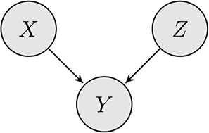
Case 1 (Collider Conflict): Let G ₁ be the basic collider structure depicted in figure 5. Suppose that we want to find the most similar causal structure in which Y has a direct causal influence on Z (rather than vice versa). According to either of our lexicographic procedures, the structure in figure 6 is uniquely most similar to G ₁ among the set of DAGs that satisfy the given constraint.

Figure 5.

Basic collider.

Figure 6.

Closest directed acyclic graph.

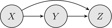
Case 2 (Adding an Arrow): Let G ₁ be the structure depicted in figure 7. Suppose that we want to find the most similar causal structure in which Y has a direct causal influence on Z (rather than there being no causal relationship between them). Both lexicographic procedures agree on a single closest structure among all those that satisfy the given constraint. Specifically, they both return the chain structure depicted in figure 8.

Figure 7.

Absent arrow.

Figure 8.

Full chain.

The fact that these three cases exist shows that there is a noteworthy class of cases for which it does not matter how we prioritize considerations of evidential and counterfactual similarity. In these cases, one might be tempted to say that there is an objective fact of the matter about what would happen were the causal structure to be different in a sense that does not exist generally; namely, no matter how considerations of evidential similarity and counterfactual similarity are prioritized, the most similar graph(s) is/are the same. Whether there are actually contexts in which each of these procedures should be used goes beyond the scope of this article, so it is still possible to argue that the resolution of every causal-structure counterfactual does not vary with context (by arguing for one of the lexicographical procedures). But since some practically minded individuals might think there are some contexts that call for one prioritization, and others that call for another, we believe that it is worth pointing out that there are some causal-structure counterfactual queries that have the same resolution no matter how things are prioritized.

6. Conclusion

We have explicated two ways in which causal structures can be similar and three ways in which these two notions of similarity can be integrated into a single master conception of similarity. We do not defend any of these master concepts as universally correct, but we have shown that there is a substantial range of cases in which they coincide. In future work we hope to explore

1. 1. When and whether there is principled reason to favor one master conception (or one system of weights) over the alternatives.

2. 2. When and whether any of these potential master conceptions can be used to assess the accuracy of causal search algorithms in terms of similarity to the true causal structure.Footnote ¹³

3. 3. Whether any of these potential master conceptions can be used to define a procedure for aggregating competing beliefs about causal structure in terms of finding the graph(s) that is/are on average most similar to the individually accepted graphs (see, e.g., Bradley, Dietrich, and List Reference Bradley, Dietrich and List2014).