2.1. Model framework

We consider a probability space $\Omega$ , endowed with a probability measure $\mathbb{P}$ , in which are defined m Markov square-integrable processes, noted $\boldsymbol{X}_{t}=\left(X_{t}^{(1)},...,X_{t}^{(m)}\right)_{t\geq0}$ , with bounded variances. These processes are the risk factors driving the value of financial assets and derivatives, managed by a financial institution. Their natural filtration is denoted by $\mathcal{F}=\left(\mathcal{F}_{t}\right)_{t\geq0}$ . If risk factors are Markov, the total asset value is a function of time and risk factors denoted by $A(t,\boldsymbol{X}_{t})$ . $\mathbb{P}$ is called the real or historical measure in rest of this article. Under the assumption of absence of arbitrage, there exists at least one equivalent risk neutral measure, denoted by $\mathbb{Q}$ , using the cash account $\left(B_{t}\right)_{t\geq0}$ as numeraire. Random asset cash flows are paid at time $\left(t_{k}\right)_{k=0,...,d}$ and denoted by $C_{k}^{A}$ . Therefore at time $t\leq t_{d}$ , $A(t,\boldsymbol{X}_{t})$ can be developed as follows:

(2.1) \begin{eqnarray}A(t,\boldsymbol{X}_{t}) & = & a\left(\boldsymbol{X}_{t}\right)+\mathbb{E}^{\mathbb{Q}}\left(\sum_{k=0}^{d}\frac{B_{t}}{B_{t_{k}}}C_{k}^{A}\,\textbf{1}_{\{t_{k}\geq t\}}|\boldsymbol{X}_{t}\right)\,,\end{eqnarray}

where $a\left(\boldsymbol{X}_{t}\right)$ is directly determined by the value of underlying risk factors. By construction, $A(t,\boldsymbol{X}_{t})$ is $\mathcal{F}_{t}-$ adapted. We assume that $A(t,\boldsymbol{X}_{t})$ is square integrable and has therefore a finite variance.

We consider a risk measure denoted by $\rho(\cdot)$ . For risk management, we aim to calculate $\rho(A(t,\boldsymbol{X}_{t}))$ . In applications, we mainly consider the value at risk (VaR) and the expected shortfall (ES). For a confidence level $\alpha\in(0,1)$ , the VaR and ES for a continuous distribution of $A(t,\cdot)$ are defined as

(2.2) \begin{align}VaR_{\alpha} & = \max\left\{ x\in\mathbb{R}\,:\,\mathbb{P}\left(A(t,\boldsymbol{X}_{t})\leq x\right)\leq\alpha\right\} \,,\end{align}

(2.3) \begin{align} ES_{\alpha} & = \frac{1}{\alpha}\int_{0}^{\alpha}VaR_{\gamma}\,d\gamma.\end{align}

The ES also admits an equivalent representation (see McNeil et al., Reference McNeil, Frey and Embrechts2015, Proposition 8.13, p. 283) that is used later for estimation:

(2.4) \begin{eqnarray}ES_{\alpha} & = & \mathbb{E}^{\mathbb{P}}\left(A(t,\boldsymbol{X}_{t})\,|\,A(t,\boldsymbol{X}_{t})\leq VaR_{\alpha}\right)\\ & = & \frac{1}{\alpha}\mathbb{E}^{\mathbb{P}}\left(A(t,\boldsymbol{X}_{t})\,\textbf{1}_{\{A(t,\boldsymbol{X}_{t})\leq VaR_{\alpha}\}}\right)\nonumber \\ & & +VaR_{\alpha}\frac{1}{\alpha}\left(1-\mathbb{P}\left(A(t,\boldsymbol{X}_{t})\leq VaR_{\alpha}\right)\right).\nonumber \end{eqnarray}

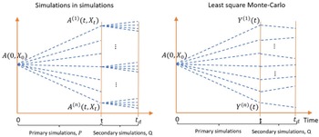
We draw the attention of the reader on the fact that VaR and ES are valued under the real measure. Computing the risk neutral expectation (2.1) is a challenging task because closed-form expressions are usually not available. A solution consists in evaluating $A(t,\boldsymbol{X}_{t})$ by simulations in simulations. This framework is illustrated in the left plot of Figure 1. For each primary simulated sample path of risk factors (under $\mathbb{P}$ ), we perform secondary simulations (under $\mathbb{Q}$ ). The value of $A(t,\boldsymbol{X}_{t})$ is next obtained by averaging the sums of discounted cash flows of secondary scenarios. This approach is nevertheless too computing intensive for being carried out with success. In practice, we rely on the method of LSMC to keep the computational time under control.

Figure 1.

Simulations in simulations versus least squares Monte Carlo.

2.2. LSMC algorithm

We briefly review the LSMC method. We denote by

\begin{eqnarray*}Y(t) & = & \sum_{k=0}^{d}\frac{B_{t}}{B_{t_{k}}}C_{k}^{A}\,\textbf{1}_{\{t_{k}\geq t\}}\,,\end{eqnarray*}

the random variable that is $\mathcal{F}_{t_{d}}$ -adapted and such that $A(t,\boldsymbol{X}_{t})=a\left(\boldsymbol{X}_{t}\right)+\mathbb{E}^{\mathbb{Q}}\left(Y(t)\,|\,\boldsymbol{X}_{t}\right)$ . This variable is called the “response” for a given set of risk factors at time t. The LSMC method is based on property that the conditional expectation of a random variable Y(t) given a random vector $\boldsymbol{X}_{t}$ minimizes the mean squared distance between Y(t) and $h(\boldsymbol{X}_{t}),$ where $h(\cdot)$ is a Borel measurable function. In practice, it means that we only need a single (or a few) secondary simulations under $\mathbb{Q}$ , as illustrated on the right plot of Figure 1. The theoretical foundation of the LSMC approach is briefly recalled in the next proposition which uses the fact that $\boldsymbol{X}_{t}$ is also $\mathcal{F}_{t_{d}}$ -adapted since $\mathcal{F}_{t}\subset\mathcal{F}_{t_{d}}$ .

Proposition 2.1. Let Y(t) be a square-integrable random variable on $\mathbb{R}$ and $\boldsymbol{X}_{t}$ an m-dimensional random vector, both $\mathcal{F}_{t_{d}}$ -adapted. The conditional expectation $\mathbb{E}^{\mathbb{Q}}\left(Y(t)\,|\,\boldsymbol{X}_{t}\right)$ is equal to $h(\boldsymbol{X}_{t})\in\mathcal{B}(\mathbb{R}^{m},\mathbb{R})$ , where $\mathcal{B}(\mathbb{R}^{m},\mathbb{R})$ is the set of Borel measurable functions from $\mathbb{R}^{m}\to\mathbb{R}$ , such that

(2.5) \begin{eqnarray}h\left(\boldsymbol{X}_{t}\right) & = & \arg\min_{h\in\mathcal{B}(\mathbb{R}^{m},\mathbb{R})}\mathbb{E}^{\mathbb{Q}}\left(\left(h\left(\boldsymbol{X}_{t}\right)-Y(t)\right)^{2}\right).\end{eqnarray}

The proof of this result is reminded in Appendix A. In many real-world applications, there is no closed-form expression for the function $h(\boldsymbol{X}_\boldsymbol{t}),$ but risk factors can be simulated under the $\mathbb{P}$ measure. Longstaff and Schwartz (Reference Longstaff and Schwartz2001) assume that the unknown function $h(\cdot)$ belongs to the $L^{2}$ -space of square-integrable functions. Since $L^{2}$ is a Hilbert space, it admits a countable orthornormal basis. The function $h(\cdot)$ may then be represented as a combination of basis functions. If $m=1$ , one common choice is the set of weighted Laguerre polynomials. In higher dimension, basis functions are usually replaced by polynomials of risk factors. In practice, the LSMC algorithm consists in simulating a sample denoted by

(2.6) \begin{align}\mathcal{S} & =\left\{ (\boldsymbol{x}_{1},y_{1}),...,(\boldsymbol{x}_{n},y_{n})\right\} \,,\end{align}

of n realizations of $\left(\boldsymbol{X}_{t},Y(t)\right)$ and in regressing responses on risk factors. We recall that $\boldsymbol{X}_{t}$ is simulated up to time t under the real measure $\mathbb{P}$ while the response Y(t) is obtained by simulations from t up to $t_{d}$ , under the risk neutral measure $\mathbb{Q}$ . Let us denote by $\mathcal{P}_{h}$ the set of polynomials $\widehat{h}(\boldsymbol{x})$ of degree $d_{h}$ approximating $h(\boldsymbol{x})$ . It is estimated by least squares minimization:

(2.7) \begin{eqnarray}\widehat{h}(.) & = & \arg\min_{\widehat{h}\in\mathcal{P}_{h}}\left(\sum_{(\boldsymbol{x}_{i},y_{i})\in\mathcal{S}}\left(y_{i}-\widehat{h}(\boldsymbol{x}_{i})\right)^{2}\right).\end{eqnarray}

Let us denote by

(2.8) \begin{align}\boldsymbol{z} & =\left(\left(x_{i_{1}}^{\,j_{1}}x_{i_{2}}^{\,j_{2}}...x_{i_{h}}^{\,j_{h}}\right)_{i_{1},...,i_{h}\in\{1,...,m\}}^{\,j_{1},...,j_{h}\in\mathbb{N},j_{1}+...+j_{h}\leq d_{h}}\right)\,,\end{align}

the vector of powers of risk factors up to order $d_{h}\in\mathbb{N}$ . We define $\widehat{h}(\boldsymbol{x})=\boldsymbol{z}^{\top}\boldsymbol{\beta}$ as a polynomial of order $d_{h}$ where $\boldsymbol{\beta}_{k}$ is a real vector of same dimension as $\boldsymbol{z}$ . The sample of powers of risk factors is $\{\boldsymbol{z}_{1},...,\boldsymbol{z}_{n}\}$ . Let us respectively denote by Z and $\boldsymbol{y}$ the matrix $Z=\left(\boldsymbol{z}_{j}^{\top}\right)_{j\in\mathcal{S}}$ and the vector $\boldsymbol{y}=\left(y_{j}\right)_{j\in\mathcal{S}}$ . Using standard arguments, the polynomial coefficients minimizing (2.7) are $\widehat{\boldsymbol{\beta}}=\left(Z^{\top}Z\right)^{-1}Z^{\top}\boldsymbol{y}$ .

Let us next denote by ${\widehat{a}_{i}}=a(\boldsymbol{x}_{i})+{\widehat{h}(\boldsymbol{x}_{i})}\approx A(t,\boldsymbol{x}_{i})$ the approximation of the value of total assets for a given vector of risk factors $\boldsymbol{X}_{t}=\boldsymbol{x}_{i}$ . The ordered sample of $\left(\widehat{a}_{i}\right)_{i=1,...,n}$ is denoted by $\left(\widehat{a}_{(i)}\right)_{i=1,...,n}$ and is such that

\[\widehat{a}_{(1)}\leq\widehat{a}_{(2)}\leq....\leq\widehat{a}_{(n)}.\]

We define $j(\alpha)$ as the indices of the $\alpha$ -quantile of $\left(\widehat{a}_{(i)}\right)_{i=1,...,n}$ :

(2.9) \begin{equation}j(\alpha)=\max\left\{ k\in\{1,...,n\}\,:\,\frac{k}{n}\leq\alpha\right\} .\end{equation}

The estimate of $VaR_{\alpha}$ is the $\alpha$ - quantile of $\left(\widehat{a}_{(i)}\right)_{i=1,...,n}$ :

\begin{align*}\widehat{VaR}_{\alpha} & =\widehat{a}_{(j(\alpha))}.\end{align*}

From Equation (2.4), the $ES_{\alpha}$ estimator is computed as follows:

\begin{align*}\widehat{ES}_{\alpha} & =\frac{1}{\alpha}\sum_{i=1}^{j(\alpha)-1}\frac{\widehat{a}_{(i)}}{n}+\widehat{a}_{(j(\alpha))}\left(1-\frac{j(\alpha)-1}{\alpha\,n}\right).\end{align*}

A critical step in the LSMC procedure is the choice of the function $\widehat{h}(\boldsymbol{X}_{t})$ that approximates the unknown conditional expectation, $h(\boldsymbol{X}_\boldsymbol{t})$ . This requires to test multiple candidate regressors and to carefully monitor potential overfit of the data set. In the next section, we propose a new approach based on local regressions.

3.1. General principles

As described above, it is a common practice to fit a global polynomial regression predicting responses $\left(y_{i}\right)_{i=1,...,n}$ as a function of risk factors $\left(\boldsymbol{x}_{i}\right)_{i=1,...n}$ . In this article, we opt for an alternative approach based on local regressions. The method is based on a finite partitioning $\left(\mathcal{Y}_{k}\right)_{k=1,...,K}$ of the domain of Y(t) (here $dom(Y(t))=\mathbb{R}$ ). Let us define

(3.1) \begin{eqnarray}h_{k}(\boldsymbol{x}) & = & \mathbb{E}^{\mathbb{Q}}\left(Y(t)\,|\,\boldsymbol{X}_{t}=\boldsymbol{x}\,,\,Y(t)\in\mathcal{Y}_{k}\right)\,,k=1,...,K,\end{eqnarray}

the conditional expectation of responses, knowing that $\boldsymbol{X}_{t}=\boldsymbol{x}$ and $Y(t)\in\mathcal{Y}_{k}$ . Using standard properties of the conditional expectation, we can rewrite the function $h(\boldsymbol{x})$ as a weighted sum of $h_{k}(.)$ :

(3.2) \begin{align}h(\boldsymbol{x}) & =\mathbb{E}^{\mathbb{Q}}\left(Y(t)\,|\,\boldsymbol{X}_{t}=\boldsymbol{x}\right)\\ & =\sum_{k=1}^{K}\mathbb{Q}\left(Y(t)\in\mathcal{Y}_{k}\,|\,\boldsymbol{X}_{t}=\boldsymbol{x}\right)h_{k}(\boldsymbol{x}).\nonumber\end{align}

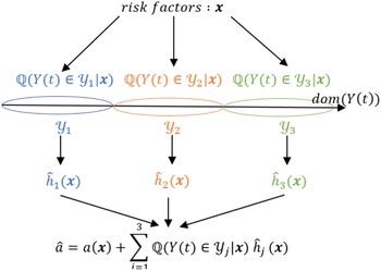
Based on this decomposition, we approximate the K unknown functions $h_{k}(\cdot)$ by polynomial regressions $\widehat{h}_{k}(\cdot)$ of $Y(t)\in\mathcal{Y}_{k}$ on risk factors. In a second step, we use a multinomial logistic regression to estimate the probabilities $\mathbb{Q}\left(Y(t)\in\mathcal{Y}_{k}\,|\,\boldsymbol{X}_{t}\right)$ for $k=1,...,K$ . Figure 2 provides a graphical representation of the LLSMC algorithm when $K=3$ . Once the model is fitted, the estimated asset value $\widehat{a}$ , for a vector of risk factors $\boldsymbol{x}$ at time t, is determined in two steps. First, we calculate the probabilities that responses belong to clusters $\left(\mathcal{Y}_{k}\right)_{k=1,...,K}$ , conditionally to $X_{t}=\boldsymbol{x}$ . Next, we compute $\widehat{h}_{k}(\boldsymbol{x})$ which approximates the conditional expectations of responses within clusters, as defined in Equation (3.1). Finally, the estimated asset value is the sum of the function $a(\boldsymbol{x})$ and of $\widehat{h}_{k}(\boldsymbol{x})$ weighted by probabilities $\mathbb{Q}\left(Y(t)\in\mathcal{Y}_{k}\,|\,\boldsymbol{X}_{t}\right)$ .

In practice, the simulated sample, $\mathcal{S}$ defined in Equation (2.6), is the union of sampled risk factors, noted $\mathcal{X}$ , and of corresponding responses $\mathcal{Y}$ . In a first stage, we partition the sample data set $\mathcal{S}=(\mathcal{X},\mathcal{Y})$ into $K\lt \lt n$ subsets, denoted by $\left(\mathcal{S}_{k}\right)_{k=1,...K}$ :

\begin{eqnarray*}\mathcal{S}_{k} & = & (\mathcal{X}_{k},\mathcal{Y}_{k})\,,\,k=1,...,K\,,\end{eqnarray*}

here $\left(\mathcal{Y}_{k}\right)_{k=1,...,k}$ is a partition of $\mathcal{Y}$ and $\left(\mathcal{X}_{k}\right)_{k=1,...,K}$ is the sample set of corresponding simulated risk factors. In this article, we use the K-means for partitioning $\mathcal{Y}$ in K clusters $\left(\mathcal{Y}_{k}\right)_{k=1,...,K}$ . As detailed in the next subsection, this heuristic algorithm computes a partition which reduces the within groups sum of squared errors or intraclass inertia.

Figure 2.

Graphical illustration of the LLSMC algorithm.

3.2. The clustering algorithm

The K-means algorithm (see MacQueen, Reference MacQueen1967 or Jain, Reference Jain2010) is based on the concept of centroids that are the center of gravity of a cluster of objects. The coordinates of the $u{\rm th}$ centroid are denoted $c_{u}\in\mathbb{R}$ , $u=1,...,K$ . If $d(\cdot,\cdot)$ is the Euclidian distance, we define the clusters $\mathcal{Y}_{k}$ for $k=1,...,K$ as follows:

(3.3) \begin{equation}\mathcal{Y}_{k}=\{y_{i}\::\:d(y_{i},c_{k})\leq d(y_{i},c_{j})\;\forall j\in\{1,...,K\}\}\quad k=1,...,K.\end{equation}

By extension, the joint cluster $\mathcal{S}_{k}$ of risk factors and responses is

(3.4) \begin{equation}\mathcal{S}_{k}=\{(\boldsymbol{x}_{i},y_{i})\::\:d(y_{i},c_{k})\leq d(y_{i},c_{j})\;\forall j\in\{1,...,K\}\}\quad k=1,...,K.\end{equation}

The center of gravity of $\mathcal{Y}_{k}$ is denoted by $g_{k}=\frac{1}{|\mathcal{Y}_{k}|}\sum_{y_{i}\in\mathcal{Y}_{k}}y_{i}$ and the center of gravity of all responses is $g=\frac{1}{n}\sum_{i=1}^{n}g_{i}$ . The global inertia is $I_{\mathcal{Y}}=\frac{1}{n}\sum_{i=1}^{n}d\left(y_{i},g\right)^{2}$ and the interclass inertia $I_{c}$ is the inertia of the cloud of centers of gravity:

\begin{eqnarray*}I_{c} & = & \sum_{k=1}^{K}\frac{|\mathcal{Y}_{k}|}{n}d\left(g_{k},g\right)^{2}.\end{eqnarray*}

The intraclass inertia $I_{a}$ is the sum of clusters inertia, weighted by their size:

\begin{eqnarray*}I_{a} & = & \frac{1}{n}\sum_{k=1}^{K}\sum_{y_{i}\in\mathcal{Y}_{k}}d\left(y_{i},g_{k}\right)^{2}.\end{eqnarray*}

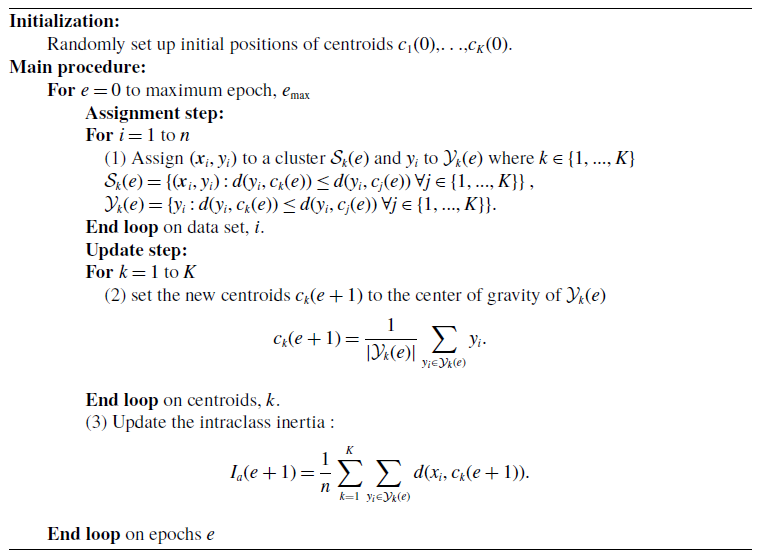
According to the König–Huyghens theorem, the global inertia is the sum of the intraclass and interclass inertia: $I_{\mathcal{Y}}=I_{c}+I_{a}$ . We seek for a partition of $\mathcal{Y}$ minimizing the intraclass inertia $I_{a}$ in order to have homogeneous clusters on average. This is equivalent to determine the partition maximizing the interclass inertia, $I_{c}$ . Finding the partition that minimizes the intraclass inertia cannot be solved numerically in polynomial time (NP-hard problem, see Mahajan et al., Reference Mahajan, Nimbhorkar and Varadarajan2012) but efficient heuristic procedures exist. The most common method uses an iterative refinement technique called the K-means which is detailed in Algorithm 2, provided in Appendix B. Given an initial set of K random centroids $c_{1}(0)$ ,…, $c_{K}(0)$ , we construct a partition $\left\{ \mathcal{Y}_{1}(0),\ldots,\mathcal{Y}_{K}(0)\right\} $ of responses. Next, we replace the K random centroids by the K centers of gravity $\left(c_{u}(1)\right)_{u=1,...,K}=\left(c_{u}(0)\right)_{u=1,...,K}$ of these classes and we iterate till convergence. At each iteration, we can prove that the intraclass inertia is reduced but we do not have any warranty that the partition found by this way is a global solution. Nevertheless, this risk is limited in our approach because we cluster unidimensional data $(y_{i=1...n}\in\mathbb{R}^{+})$ . As dimensionality increases, the distance to the nearest neighbor approaches the distance to the farthest neighbor but for one dimension data, K-means is highly efficient as discussed in Beyer et al. (Reference Beyer, Goldstein, Ramakrishnan and Shaft1999). In numerical illustrations, we use an improved version of the algorithm, the K-means++ of Arthur and Vassilvitskii (Reference Arthur and Vassilvitskii2007). This enhances the quality of the resulting clusters by providing initial centroids that are well spread out across the data space. The initial centroids are selected in a probabilistic manner based on their distance from already chosen centroids. In practice, this procedure is repeated several times (20 times in this article) and we keep the partition with the lowest intraclass inertia. Notice that there exists a large variety of clustering methods (Gaussian mixture model (GMM), DBscan, spectral K-means, etc.) that are substitutable to the K-means. The impact is nevertheless limited given that we cluster unidimensional data. In the first case study, we have indeed replaced the K-means algorithm by the GMM and have not observed any significant differences.

3.3. Local regressions

After having found a partition of $\mathcal{S}$ in $\mathcal{S}_{k}=(\mathcal{X}_{k},\mathcal{Y}_{k})\,,\,k=1,...,K\:,$ we approximate functions $\left(h_{k}\right)_{k=1,...,K}$ by K polynomials of order $d_{h}$ , denoted by $\left(\widehat{h}_{k}(\cdot)\right)_{k=1,...,K}$ . Let us recall that $\boldsymbol{z}$ as defined in Equation (2.8) is the vector of powers of risk factors up to $d_{h}\in\mathbb{N}$ . We assume that $\widehat{h}_{k}(\boldsymbol{x})=\boldsymbol{z}^{\top}\boldsymbol{\beta}_{k}$ is a polynomial of order $d_{h}$ where $\boldsymbol{\beta}_{k}$ is a real vector of dimension equal to the one of $\boldsymbol{z}$ . In a similar manner to LSMC, the $\left(\widehat{h}_{k}(\cdot)\right)_{k=1,...,K}$ are estimated by least squares minimization over the set $\mathcal{P}_{h}$ of polynomials of degree $d_{h}$ :

(3.5) \begin{eqnarray}\boldsymbol{\beta}_{k} & = & \arg\min_{\widehat{h}_{k}\in\mathcal{P}_{h}}\left(\sum_{(\boldsymbol{x}_{i},y_{i})\in\mathcal{S}_{k}}\left(y_{i}-\widehat{h}_{k}(\boldsymbol{x}_{i})\right)^{2}\right).\end{eqnarray}

The sample of powers of risk factors is again $\{\boldsymbol{z}_{1},...,\boldsymbol{z}_{n}\}$ and we denote by $Z_{k}$ and $\boldsymbol{y}_{k}$ the matrix $Z_{k}=\left(\boldsymbol{z}_{j}^{\top}\right)_{j\in\mathcal{S}_{k}}$ and the vector $\boldsymbol{y}_{k}=\left(y_{j}\right)_{j\in\mathcal{S}_{k}}$ for $k=1,...,K$ . Using standard arguments, the polynomial coefficients minimizing (3.5) are $\widehat{\boldsymbol{\beta}}_{k}=\left(Z_{k}^{\top}Z_{k}\right)^{-1}Z_{k}^{\top}\boldsymbol{y}_{k}$ .

Algorithm 1:

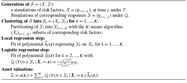
Summary of the LLSMC estimation procedure.

Nevertheless, this model is useless for predicting the response for a vector $\boldsymbol{x}$ that is not in the training data set. For $\boldsymbol{x}\notin\mathcal{S}$ , the expected response should be

(3.6) \begin{align}\widehat{h}(\boldsymbol{x}) & =\sum_{k=1}^{K}\mathbb{Q}\left(Y(t)\in\mathcal{Y}_{k}\,|\,\boldsymbol{X}_{t}=\boldsymbol{x}\right)\widehat{h}_{k}(\boldsymbol{x})\,,\end{align}

where $\mathbb{Q}\left(Y(t)\in\mathcal{Y}_{k}\,|\,\boldsymbol{X}_{t}=\boldsymbol{x}\right)$ is the unknown probability that the response for $\boldsymbol{x}$ is in the $k^{th}$ cluster. We estimate these probabilities with a multinomial logistic regression. In this framework, we assume that conditional probabilities are the following functions:

(3.7) \begin{eqnarray}\mathbb{Q}\left(Y(t)\in\mathcal{Y}_{k}\,|\,\boldsymbol{X}_{t}=\boldsymbol{x}\right) & = & \begin{cases}\frac{e^{-\widehat{\boldsymbol{\gamma}}_{k}(\boldsymbol{x})}}{1+\sum_{j=2}^{K}e^{-\widehat{\boldsymbol{\gamma}}_{j}(\boldsymbol{x})}} & k=2,...,K\,,\\\frac{1}{1+\sum_{j=2}^{K}e^{-\widehat{\boldsymbol{\gamma}}_{j}(\boldsymbol{x})}} & k=1\,,\end{cases}\end{eqnarray}

where $\widehat{\gamma}_{k}(\boldsymbol{x})$ is a polynomial of risk factors approximating the unknown exact function $\gamma_{k}(\boldsymbol{x})$ . If $\mathcal{P}_{\gamma}$ is the set of admissible polynomial functions of order $d_{\gamma}\in\mathbb{N}$ , the $\left(\widehat{\gamma}_{k}(\cdot)\right)_{k=2,...,K}$ are estimated by log-likelihood maximization. We denote by

\begin{align*}\boldsymbol{w} & =\left(\left(x_{i_{1}}^{\,j_{1}}x_{i_{2}}^{\,j_{2}}...x_{i_{h}}^{\,j_{h}}\right)_{i_{1},...,i_{h}\in\{1,...,m\}}^{j_{1},...,j_{h}\in\mathbb{N},j_{1}+...+j_{h}\leq d_{\gamma}}\right)\end{align*}

the vector of powers of risk factors up to $d_{\gamma}\in\mathbb{N}$ . We assume that $\widehat{\gamma}_{k}(\boldsymbol{x})=\boldsymbol{w}^{\top}\boldsymbol{\zeta}_{k}$ is a polynomial of order $d_{\gamma}$ where $\boldsymbol{\zeta}_{k}$ is a real vector of same dimension as $\boldsymbol{w}$ . The log-likelihood is defined by

\begin{eqnarray*}\mathcal{L}\left(\left(\gamma_{k}\right)_{k=2,...,K}\right) & = & \sum_{i=1}^{n}\log\left(\sum_{k=2}^{K}\frac{\textbf{1}_{\{y_{i}\in\mathcal{Y}_{k}\}}e^{-\boldsymbol{\gamma}_{k}(\boldsymbol{x}_{i})}}{1+\sum_{j=2}^{K}e^{-\boldsymbol{\gamma}_{j}(\boldsymbol{x}_{i})}}+\frac{\textbf{1}_{\{y_{i}\in\mathcal{Y}_{1}\}}}{1+\sum_{j=2}^{K}e^{-\boldsymbol{\gamma}_{j}(\boldsymbol{x})}}\right)\,,\end{eqnarray*}

and $\left(\boldsymbol{\zeta}_{k}\right)_{k=2,...,K}=\arg\max_{\gamma_{k}\in\mathcal{P}_{\gamma}}\mathcal{L}\left(\left(\gamma_{k}\right)_{k=2,...,K}\right)$ . The full procedure to fit the LLSMC is summarized into Algorithm 1. We first simulate $\mathcal{S}=\left(\mathcal{X},\mathcal{Y}\right)$ and create clusters on which we fit local polynomial regressors by least squares minimization. Next, we estimate conditional probabilities (3.7) and compute asset values.

In a similar manner to Cheridito et al. (Reference Cheridito, Ery and Wüthrich2020), we can replace the polynomial functions $\widehat{\gamma}_{k}(\boldsymbol{x})$ by neural networks or by any other machine learning regressor.

At this stage, we have not discussed yet the convergence of the LLSMC. The framework is based on the Equality (3.2) that is true whatever the number of clusters. The question of convergence arises from the approximations of $\mathbb{Q}\left(Y(t)\in\mathcal{Y}_{k}\,|\,\boldsymbol{x}\right)=\frac{e^{-\gamma_{k}(\boldsymbol{x})}}{1+\sum_{j=2}^{K}e^{-\gamma_{j}(\boldsymbol{x})}}$ and $h_{k}(\boldsymbol{x})$ by a logistic and polynomial regressions. If functions $\gamma_{k}(\boldsymbol{x})$ and $h_{k}(\boldsymbol{x})$ are $C^{\infty}$ , the Taylor’s theorem ensures the (local) convergence when the polynomial orders $d_{h}$ and $d_{\gamma}$ $\to\infty$ .

If a set of $L^{2}$ -orthogonal basis functions $\left(e_{j}(\boldsymbol{x})\right)_{j\in\mathbb{N}}$ from $\mathbb{R}^{p}$ to $\mathbb{R}$ is well defined, an alternative is to approximate $h_{k}(\boldsymbol{x})$ and $\gamma_{k}(\boldsymbol{x})$ by a finite combination of m basis functions:

\begin{align*}\widehat{h}_{k}(\boldsymbol{x}) & =\sum_{j=1}^{m}\alpha_{k,j}e_{j}(\boldsymbol{x})\quad,\quad\gamma_{k}(\boldsymbol{x})=\sum_{j=1}^{m}\beta_{k,j}e_{j}(\boldsymbol{x})\,,\end{align*}

for $k=1,...,K$ . In this case, the convergence is guaranteed when $m\to\infty$ . Nevertheless, finding such an orthogonal basis function $\left(e_{j}(\boldsymbol{x})\right)_{j\in\mathbb{N}}$ is a challenging task and we refer the reader to Ha and Bauer (Reference Ha and Bauer2022) for details. This motivate us to opt for polynomial approximations.

3.4. Measures of goodness of fit

We have not discussed yet how to optimize the number of clusters K and the polynomial orders, $d_{h}$ , $d_{\gamma}$ . In practice, we check four indicators of goodness of fit. We first compare the $R^{2}$ for different settings. The $R^{2}$ is the percentage of variance of responses explained by the model:

(3.8) \begin{equation}R^{2}=1-\frac{\sum_{i=1}^{n}\left(y_{i}-\widehat{h}(\boldsymbol{x}_{i})\right)^{2}}{\sum_{i=1}^{n}\left(y_{i}-\bar{y}\right)^{2}}\,,\end{equation}

where $\bar{y}=\frac{1}{n}\sum_{i=1}^{n}y_{i}$ . In LSMC regression, responses y are by construction noised estimates of $\mathbb{E}^{\mathbb{Q}}\left(Y(t)\,|\,\boldsymbol{x}\right),$ and therefore, the $R^{2}$ is by nature small. We assess the fit of local regressions by

(3.9) \begin{equation}R_{loc}^{2}=1-\frac{\sum_{k=1}^{K}\sum_{(\boldsymbol{x}_{i},y_{i})\in\mathcal{S}_{k}}\left(y_{i}-\widehat{h}_{k}(\boldsymbol{x}_{i})\right)^{2}}{\sum_{i=1}^{n}\left(y_{i}-\bar{y}\right)^{2}}.\end{equation}

Contrary to $R^{2}$ , we may expect a $R_{loc}^{2}$ close to 1 and should exclude any models with a low $R_{loc}^{2}$ . The $R^{2}$ and $R_{loc}^{2}$ both increase with the complexity of the model, measured by the number of its parameters. For this reason, we also compute a second indicator of goodness of fit which is the mean squared error of residuals:

(3.10) \begin{equation}MSE=\frac{\sum_{i=1}^{n}\left(y_{i}-\widehat{h}(\boldsymbol{x})\right)^{2}}{n-p}\,,\end{equation}

where p is the number of regression parameters. This criterion tends to penalize models with a large number of parameters. To detect abnormal prices, we calculate the sum of squared errors between exact values of $A(t,\boldsymbol{x})$ and their LLSMC estimates, $h(\boldsymbol{x})$ over a small sample of risk factors. We call this sample the validation set and denote it by $\mathcal{V}$ . Depending upon the nature of assets, the exact values of $A(t,\boldsymbol{x}_{t})$ are computed by performing a sufficient number of secondary simulations or by any other suitable numerical method. This step being computationally intensive, the size of the validation set, must be limited but should contain sufficiently diversified combinations of risk factors. A simple approach consists in combining quantiles of risk factors. Let us detail this approach. We denote by $\left(x_{(i)}^{(k)}\right)_{i=1,...,n}$ the ordered sample $\left(x_{i}^{(k)}\right)_{i=1,...,n}$ of the $k^{th}$ risk factor:

\[x_{(1)}^{(k)}\leq x_{(2)}^{(k)}\leq...\leq x_{(n)}^{(k)}.\]

We select a small number of $q\in\mathbb{N}$ quantiles $\left(x_{j(\alpha_{1})}^{(k)},...,x_{j(\alpha_{q})}^{(k)}\right)$ where $\left(\alpha_{i}\right)_{i=1,...,q}$ are probabilities and $j(\alpha_{i})$ is the quantile index such as defined in Equation (2.9). We repeat this operation for each $k=1,...,m$ . The validation set $\mathcal{V}$ contains all the combination of quantiles and its total size is $|\mathcal{V}|=q^{m}$ . The MSE on the validation sample is

(3.11) \begin{equation}MSE(\mathcal{V})=\frac{1}{|\mathcal{V}|}\sum_{\boldsymbol{x}\in\mathcal{V}}\left(A(t,\boldsymbol{x})-\widehat{h}(\boldsymbol{x})\right)^{2}.\end{equation}

If the dimension of $|\mathcal{V}|$ is too large, we can select randomly a subset of $\mathcal{V}$ . Besides the analysis of these indicators of goodness of fit, it is recommended to plot the function $\widehat{h}(\boldsymbol{x})$ to detect unexpected tail behaviors. If the asset value is computable in a large number of scenarios, we can appraise the goodness of fit by divergence measures (e.g. Kullback–Leibler) between distributions of $A(t,\boldsymbol{x})$ and $\widehat{h}(\boldsymbol{x})$ , approached by simulations of $\boldsymbol{x}$ . Nevertheless, this approach is in most of cases computationally intensive.

3.5. Simpson’s paradox

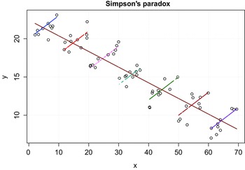
It may appear counterintuitive to partition the data set using responses instead of risk factors. Two reasons motivate this choice. First, local regressions based on hard clustering of risk factors produce discontinuities in predictions, $\mathbb{E}^{\mathbb{Q}}\left(Y(t)\,|\,\boldsymbol{X}_{t}\right)$ , on borders of clusters, even in a market in which all risk factors are continuous. This is clearly an undesirable feature for a model designed for risk management. Second, this prevents to observe the Simpson’s paradox (Simpson, Reference Simpson1951). This is a phenomenon in probability and statistics in which a trend appears in several groups of data but disappears or reverses when the groups are combined. This paradox is illustrated in Figure 3 which compares local versus global linear regressions. Regressions on clusters of $\boldsymbol{x}$ detect misleading local increasing trends, whereas the slope of the global model is negative. We provide a financial illustration of the Simpson’s paradox in the first case study.

Figure 3.

Illustration of the Simpson’s paradox.

4.1. The Heston model

In the Heston model, the cash account earns a constant risk free rate r. The stock price, noted $\left(S_{t}\right)_{t\geq0}$ , is ruled by a geometric Brownian diffusion with a stochastic variance, $\left(V_{t}\right)_{t\geq0}$ :

(4.1) \begin{equation}\begin{cases}dS_{t} & =\mu\,S_{t}\,dt+S_{t}\sqrt{V_{t}}\left(\rho dW_{t}^{v}+\sqrt{1-\rho^{2}}dW_{t}^{s}\right)\,,\\dV_{t} & =\kappa\left(\gamma-V_{t}\right)dt+\sigma\sqrt{V_{t}}dW_{t}^{v}.\end{cases}\end{equation}

where $\left(W_{t}^{s}\right)_{t\geq0}$ and $\left(W_{t}^{v}\right)_{t\geq0}$ are independent Brownian motions defined on the real probability space $\left(\Omega,\mathcal{F},\mathbb{P}\right)$ . $\mu\in\mathbb{R}$ is the expected instantaneous stock return and $\rho\in({-}1,1)$ is the correlation between the price and volatility. The variance reverts with a speed $\kappa>0$ to a mean reversion level $\gamma\gt 0$ . The volatility of the variance is a multiple $\sigma\in\mathbb{R}^{+}$ of the square root of variance.

For the sake of simplicity, we assume that the variance has the same dynamics under $\mathbb{P}$ and $\mathbb{Q}$ (this assumption may be relaxed without any impact on our analysis), whereas the drift of the stock price is replaced by the risk free rate under $\mathbb{Q}$ .

Table 1.

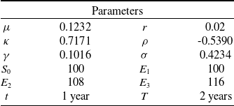
Parameters of the Heston stochastic volatility model and of the payoff.

There is no analytical formula for option prices in the Heston model. Nevertheless, the characteristic function of log-returns admits a closed-form expression and we can calculate their probability density function (pdf) by DFT. European options are then valued by computing the expected discounted payoff with this pdf. Prices obtained by DFT are compared to these obtained with LSMC and LLSMC methods. Details about the pricing method are available in the Online Supplementary Materials.

4.2. Butterfly options

In order to apply the LSMC to the Heston model, we consider as risk factors the normed stock price and volatility:

\begin{align*}\boldsymbol{X}_{t} & :=\left(\frac{S_{t}-\mathbb{E}_{0}^{\mathbb{P}}\left(S_{t}\right)}{\sqrt{\mathbb{V}_{0}^{\mathbb{P}}\left(S_{t}\right)}},\frac{\sqrt{V_{t}}-\mathbb{E}_{0}^{\mathbb{P}}\left(\sqrt{V_{t}}\right)}{\sqrt{\mathbb{V}_{0}^{\mathbb{P}}\left(\sqrt{V_{t}}\right)}}\right).\end{align*}

In practice, expectations and variances of $S_{t}$ and $\sqrt{V_{t}}$ are estimated by empirical averages and variances of the simulated sample. We consider a European butterfly option of maturity T and strikes $E_{1}$ , $E_{2,}$ and $E_{3}$ . The payoff of this option is

\[H(S_{T})=\left(S_{T}-E_{1}\right)_{+}-2\left(S_{T}-E_{2}\right)_{+}+\left(S_{T}-E_{3}\right)_{+},\]

and its price $A(t,\boldsymbol{X}_{t})$ , at time $t\leq T$ , is equal to the $\mathbb{Q}-$ expected discounted payoff, $A(t,\boldsymbol{X}_{t})=\mathbb{E}^{\mathbb{Q}}\left(e^{-r(T-t)}H(S_{T})\,|\,\mathcal{F}_{t}\right)$ . We choose this derivative because its payoff presents three inflection points and is not an invertible function with respect to stock prices. As we will see, the price of such an option is difficult to replicate with the LSMC. We will next consider a bull trap option which has an increasing payoff. Table 1 reports model and payoff parameters. The Heston model is fitted to the time series of the S&P 500 from 31/1/2001 to 31/1/2020 by Bayesian log-likelihood maximization (for details on the estimation procedure, see Hainaut, Reference Hainaut2022, p. 75). We perform 10,000 primary simulations of $S_{t}$ and $V_{t}$ under $\mathbb{P}$ up to $t=1$ year. For each primary simulation, we simulate a single secondary sample path under $\mathbb{Q}$ up to $T=2$ years. We consider 350 steps of time per year and responses are equal to $Y(t)=e^{-r(T-t)}H(S_{T})$ .

4.3. Numerical analysis of LSMC and LLSMC

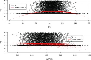
The upper and lower plots of Figure 4 depict the simulated responses plotted against stock prices and volatilities. The red points represent the LSMC estimates of butterfly option prices 1 year ahead, using a second-order polynomial of risk factors. These graphs expose a limitation of the conventional LSMC approach: it is unable to predict a positive option price for extremely high and low values of stock prices. This issue is particularly significant when using LSMC for computing risk measures.

Figure 4.

Simulated responses $Y(t)=e^{-r(T-t)}H(S_{T})$ versus stock prices, $S_{t}$ , and volatilities, $\sqrt{V_{t}}$ . The red points are the predictions $h(\boldsymbol{X}_{t})$ from the LSMC with a second-order polynomials regression.

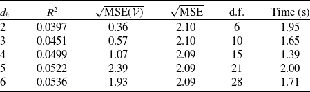
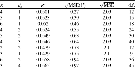
Table 2 reports the $R^{2}$ , the MSE, and MSE $(\mathcal{V})$ of the LSMC, such as defined by Equations (3.8), (3.10), and (3.11). The validation set counts 100 pairs of risk factors. We consider $q=10$ empirical quantiles of stock prices and volatilities for probabilities from 1% to 5% and from 95% to 99% by step of 1%. This choice is motivated by the observation that extreme values of risk factors tend to produce extremely high and low option prices. The exact prices of butterfly options in these 100 scenarios are computed by DFT.

Table 2.

$R^{2}$ , MSE, MSE $(\mathcal{V}),$ and runtimes of regressions of $Y_{t}$ on $\boldsymbol{X}_{t}$ in the LSMC model. d.f. is the number of parameters.

In Table 2, butterfly prices are approached by polynomial regressions of order $d_{h}$ from 2 to 6. As expected, $R^{2}$ s are tiny since responses are noised estimates of $\mathbb{E}^{\mathbb{Q}}\left(Y(t)\,|\,\boldsymbol{x}\right)$ . The $R^{2}$ s also increase with the complexity of the model. The MSE on the training set is nearly constant whatever the polynomial order, whereas the lowest MSE $(\mathcal{V})$ on the validation set is achieved with an order 2 polynomial. The LSMC is estimated in less than 2 s.Footnote 1 We next analyze the tail behavior of these approximations. This is done by plotting the function $\widehat{h}(\boldsymbol{x})$ . We will come back on this point later and focus first on the LLSMC.

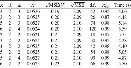
Table 3 presents the statistics of goodness of fit for the LLSMC model. The number of clusters, K, varies from 2 to 6. We test polynomials of degrees $d_{h}$ from 2 to 4 and $d_{\gamma}$ equal to 1 and 2. Models are sorted by increasing MSE $(\mathcal{V})$ s and we report statistics of the 10 first best models according to this criterion.

Table 3.

$R^{2}$ , MSE, MSE $(\mathcal{V})$ , $R_{loc,}^{2}$ and runtimes for the LLSMC model. d.f. is the number of parameters.

The optimal goodness of fit is achieved by using three clusters, applying cubic regression to each cluster, and utilizing a second-order polynomial for the multinomial logistic regression. Upon comparing the results with the LSMC figures in Table 2, it is evident that the LLSMC method significantly reduces the mean squared error MSE $(\mathcal{V})$ on the validation data set, while the MSEs on the training set remain comparable. This indicates that the LLSMC model better replicates extremely high and low option prices. It is worth noting that the LLSMC- LLSMC- and LSMC- $R^{2}$ values are comparable. The runtime for the LLSMC method ranges from 4.28 to 5.59 s.

We provide in the Online Supplementary Materials the goodness of fit statistics and runtimes for the LSMC and LLSMC, computed with 100,000 simulations instead of 10,000. A comparison with Tables 2 and 3 does not reveal any significant increases of MSE and $R^{2}$ . This validates our choice to limit the number of scenarios to 10,000.

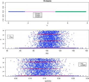
We compare the LSMC and the LLSMC with hyperparameters $K=3$ , $d_{\gamma}=2$ , $d_{h}=3$ (denoted by LLSMC 3-2-3) as this setting leads to a low MSE $(\mathcal{V})$ and a high $R_{loc}^{2}$ . The upper plot of Figure 5 shows the segmentation of responses in 3 clusters with the K-means algorithm. The mid and lower plots show the responses and local predictions $\widehat{h}_{k}(\boldsymbol{X}_{t})$ (red points) on clusters, with respect to stock prices and volatilities. In contrast to the LSMC approach, the LLSMC method does not produce significant negative responses.

Figure 5.

Upper plot: a-priori segmentation of responses in three clusters. Mid and lower plots: responses (blue points) and local regressions (red points) with respect to stock prices and volatilities.

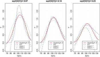
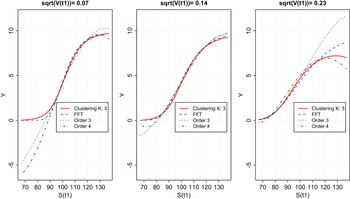
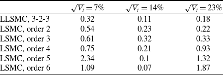
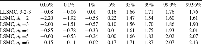
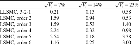
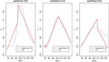
Figure 6 compares LSMC and LLSMC butterfly options for stock prices $S_{t}$ ranging from 68 to 139, the 1% and 99% percentiles of simulated stock prices and $\sqrt{V_{t}}\in\{7\%,14\%,23\%\}$ , and the 1%, 50%, and 99% quantiles of simulated volatilities. Exact option prices are computed by DFT with $u_{\max}=2$ and $M=2^{8}$ steps of discretization. The middle plot illustrates the option prices under standard market conditions, while the right and left plots represent extreme volatility conditions. We observe that LSMC models of order 2 or 4 produce negative prices in the tails. To evaluate the overall accuracy of methods in these three scenarios of volatility, we provide in Table 4 the average pricing errors. This table confirms that the LLSMC globally outperforms LSMC. Tables 5 and 6 present the VaRs and TVaRs of the butterfly option for various quantiles. The LSMC models yield negative values for the lowest percentiles, whereas the LLSMC provides slightly lower VaRs and TVaRs than the LSMC of orders 3–6 for the highest percentiles. It would be interesting to compare these results to VaRs and TVaRs based on exact prices computed by DFT. Unfortunately, the valuation by DFT of 10,000 butterfly options is computationally intensive. Nonetheless, such a comparison is feasible in the second case (Section 5).

Figure 6.

Butterfly options for $S_{t}$ ranging from 68 to 139 and volatilities $\sqrt{V_{t}}\in\{7\%,14\%,23\%\}$ .

Table 4.

Average pricing errors for the three cases presented in Figure 5.

Table 5.

VaR 1 year, LSMC model, and LLSMC.

Table 6.

Expected shortfall, 1 year, LSMC model, and LLSMC.

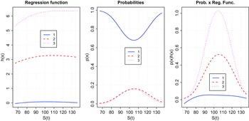
We provide a detailed explanation of how the LLSMC 3-2-3 method operates, using Figure 7. The left plot shows the local regression functions $\widehat{h}_{k}(x)$ , for various stock prices $S_{t}$ and a volatility of 14%. The middle plot depicts the probabilities that a pair of risk factors leads to a response belonging to the $k{\rm th}$ cluster. The first cluster explains the left and right tails of butterfly option prices. When $S_{t}$ is below 80 or above 130, the response is assigned to cluster 1 with a probability exceeding 90% and the correspond function $\widehat{h}_{3}(\boldsymbol{x})$ is nearly flat and close to zero. The probabilities of belonging to clusters 2 and 3 are relatively similar and exceed 5% for $S_{t}\in[80,130]$ . The right plot displays the products of the regression and probabilities functions. According to Equation (3.6), the estimated option price is obtained by summing of these three terms.

Figure 7.

Plots of regression functions $h_{k}(\boldsymbol{x})$ for $k=1,...,K$ , probabilities $\mathbb{Q}\left(Y(t)\in\mathcal{Y}_{k}\,|\,\boldsymbol{X}_{t}=\boldsymbol{x}\right),$ and their products, for $\sqrt{V_{t}}=14\%$ .

4.4. Bull trap options

We have considered a butterfly option because its payoff is not strictly increasing or decreasing function of $S_{T}$ . In this paragraph, we check that the LLSMC still outperforms the LSMC for increasing payoffs. We consider a long and a short position in call options of maturity T and strikes $E_{1}$ , $E_{2}$ . The total payoff of this bull trap option is equal to

\[H(S_{T})=\left(S_{T}-E_{1}\right)_{+}-\left(S_{T}-E_{2}\right)_{+}.\]

We use the same parameters of Table 1, except that we set strikes to $E_{1}=100$ , $E_{2}=110$ . We compare the LSMC and the LLSMC with hyperparameters $K=3,$ $d_{\gamma}=2$ , $d_{h}=1$ . Figure 7 compares LSMC and LLSMC bull trap options for stock prices $S_{t}$ ranging from 68 to 139, and $\sqrt{V_{t}}\in\{7\%,14\%,23\%\}$ . Table 7 presents the average pricing errors in the three scenarios. These results provide confirmation that the LLSMC method achieves a higher level of overall accuracy compared to the LSMC method.

Table 7.

Average pricing errors, bull trap portfolio.

4.5. Partitioning of risk factors and the Simpson’s paradox

To conclude this section, we illustrate the Simpson’s paradox in butterfly option pricing. For this purpose, we divide the sample $\mathcal{S}$ into $K\lt \lt n$ subsets $\left(\mathcal{S}_{k}\right)_{k=1,...K}$ :

\begin{eqnarray*}\mathcal{S}_{k} & = & (\mathcal{X}_{k},\mathcal{Y}_{k})\,,\,k=1,...,K\,,\end{eqnarray*}

where the partition is based on the pooling of risk factors. Each cluster is defined by a centroid $\boldsymbol{c}_{k}\in\mathbb{R}^{m}$ of dimension m such that

\[\mathcal{S}_{k}=\{(\boldsymbol{x}_{i},y_{i})\::\:d(\boldsymbol{x}_{i},\boldsymbol{c}_{k})\leq d(\boldsymbol{x}_{i},\boldsymbol{c}_{j})\;\forall j\in\{1,...,K\}\}\quad k=1,...,K.\]

We use the K-means algorithm to find the partition of $\mathcal{S}$ in $\mathcal{S}_{k}=(\mathcal{X}_{k},\mathcal{Y}_{k})\,,\,k=1,...,K$ . The conditional expectation of responses is approached by a piecewise function

\begin{align*}\widehat{h}(\boldsymbol{x}) & =\sum_{k=1}^{K}\textbf{1}_{\{\boldsymbol{x}\in\mathcal{S}_{k}\}}\widehat{h}_{k}(\boldsymbol{x})\,,\end{align*}

where $\widehat{h}_{k}\in\mathcal{P}_{h}$ is the set of polynomials of order $d_{h}$ . As for a LLSMC regression, the $\widehat{h}_{k}$ are estimated by least squares minimization (Equation (2.4)). This variant of local model is denoted by $\mathcal{X}$ -LLSMC.

Table 8 provides statistics of goodness of fit for models with K ranging from 2 to 6 and $d_{h}$ from 1 to 4. Models are sorted in ascending order of MSE $(\mathcal{V})$ s and the table displays statistics of the 10 best models according to this criterion. Compared to Table 3, the $\mathcal{X}$ -LLSMC 4-1 achieves a similar accuracy with less parameters. If we restrict our analysis to a comparison of goodness of fit statistics, both the $\mathcal{X}$ -LLSMC and LLSMC methods appear to be equivalent for computing VaR or TVaR. Plotting the $\mathcal{X}$ -LLSMC regression function leads to another conclusion. Figures 8 and 9 compares $\mathcal{X}$ -LLSMC 4-1 and DFT Butterfly prices for $S_{t}$ ranging from 68 to 139, and $\sqrt{V_{t}}\in\{7\%,14\%,23\%\}$ . We observe that local regressions based on clusters of risk factors produce discontinuities in predicted responses on borders of clusters. Second, we identify local trends not relevant to the global slope of price curves. These two elements disqualify the $\mathcal{X}$ -LLSMC for risk management purposes.

Figure 8.

Bull trap options for $S_{t}$ ranging from 68 to 139 and volatilities $\sqrt{V_{t}}\in\{7\%,14\%,23\%\}$ .

Figure 9.

Butterfly options for $S_{t}$ ranging from 68 to 139 and volatilities $\sqrt{V_{t}}\in\{7\%,14\%,23\%\}$ .

Table 8.

$R^{2}$ , MSE, MSE $(\mathcal{V}),$ and $R_{loc}^{2}$ for the $\mathcal{X}$ -LLSMC model. d.f. is the number of parameters.

5.1. A participating pure endowment

We consider a joint life insurance and financial market. The stock price indices, the interest rate, and the force of mortality are, respectively, denoted by $\left(S_{t}\right)_{t\geq0}$ , $\left(r_{t}\right)_{t\geq0,}$ and $\left(\mu_{x+t}\right)_{t\geq0}$ . These processes are defined on a probability space $\left({{\Omega}},\mathcal{F},\mathbb{P}\right)$ by the following dynamics:

(5.1) \begin{eqnarray}\left(\begin{array}{c}dS_{t}\\dr_{t}\\d\mu_{x+t}\end{array}\right) & = & \left(\begin{array}{c}\mu\,S_{t}\\\kappa_{r}\left(\gamma_{r}(t)-r_{t}\right)\\\kappa_{\mu}\left(\gamma_{x}(t)-\mu_{x+t}\right)\end{array}\right)dt+\left(\begin{array}{ccc}S_{t}\sigma_{S} & 0 & 0\\0 & \sigma_{r} & 0\\0 & 0 & \sigma_{x}(t)\end{array}\right)\Sigma\left(\begin{array}{c}dW_{t}^{(1)}\\dW_{t}^{(2)}\\dW_{t}^{(3)}\end{array}\right).\end{eqnarray}

$\left(W_{t}^{(1)},W_{t}^{(2)},W_{t}^{(3)}\right)_{t\geq0}$ are independent Brownian motions. $\mu$ , $\kappa_{r}$ , $\kappa_{\mu}$ , $\sigma_{S,}$ and $\sigma_{r}$ belong to $\mathbb{R}^{+}$ , whereas $\gamma_{r}(t)$ , $\gamma_{x}(t)$ , and $\sigma_{x}(t)$ are positive functions of time. $\gamma_{r}(t)$ and $\gamma_{x}(t)$ are fitted to term structures of interest and mortality rates. The initial age of the insured is denoted by $x\in[0,x_{\max})$ , $x_{\max}\gt 0$ . Furthermore, we assume that the standard deviation of mortality is related to age through the relation $\sigma_{x}(t)=\alpha e^{\beta(x+t)}$ . Details about $\gamma_{x}(t)$ and $\sigma_{x}(t)$ are provided in the Online Supplementary Materials. The matrix $\Sigma$ is the (upper) Cholesky decomposition of the correlation matrix and is such that

\begin{eqnarray*}\Sigma & = & \left(\begin{array}{c@{\quad}c@{\quad}c}\epsilon_{SS} & \epsilon_{Sr} & \epsilon_{S\mu}\\0 & \epsilon_{rr} & \epsilon_{r\mu}\\0 & 0 & 1\end{array}\right),\quad\left(\begin{array}{c@{\quad}c@{\quad}c}1 & \rho_{Sr} & \rho_{S\mu}\\\rho_{Sr} & 1 & \rho_{r\mu}\\\rho_{S\mu} & \rho_{r\mu} & 1\end{array}\right)=\Sigma\Sigma^{\top}\,,\end{eqnarray*}

where $\rho_{Sr,}\,\rho_{S\mu}$ and $\rho_{r\mu}\in({-}1,1)$ . This model incorporates the correlation between financial and mortality shocks, which can be relevant in the context of events such as a pandemic like Covid-19. It is worth noting that Ha and Bauer (Reference Ha and Bauer2022) have also explored a similar framework, although our model differs in terms of mortality dynamics, where we incorporate mean reversion with age-dependent volatility. Additionally, our focus is on benchmarking the LLSMC algorithm using a participating pure endowment contract, for which we derive a closed-form expression for its price. The contract which is subscribed by an individual of age x guarantees a payout at the expiry date (T) equal to the maximum between a capital $C_{T}$ and the stock indices $S_{T}$ , in the event of survival. However, the benefit is upper bounded by $C_{M}$ . If we denote by $\tau\in\mathbb{R}^{+}$ the random time of insured’s death, the value of such a policy is equal to the expected discounted cash flows under the chosen risk neutral measure:

(5.2) \begin{eqnarray} & & V_{t}=\mathbb{E}^{\mathbb{Q}}\left(e^{-\int_{t}^{T}r_{s}ds}\textbf{1}_{\{\tau\geq T\}}\left(C_{T}+\left(S_{T}-C_{T}\right)_{+}-\left(S_{T}-C_{M}\right)_{+}\right)\,|\,\mathcal{F}_{t}\right)\\ & & \quad=\textbf{1}_{\{\tau\geq t\}}C_{T}\mathbb{E}^{\mathbb{Q}}\left(e^{-\int_{t}^{T}(r_{s}+\mu_{x+s})ds}\,|\,\mathcal{F}_{t}\right)\nonumber \\ & & \quad\,+\textbf{1}_{\{\tau\geq t\}}\mathbb{E}^{\mathbb{Q}}\left(e^{-\int_{t}^{T}(r_{s}+\mu_{x+s})ds}\left(\left(S_{T}-C_{T}\right)_{+}\right)\,|\,\mathcal{F}_{t}\right)\nonumber \\ & & \quad\,-\textbf{1}_{\{\tau\geq t\}}\mathbb{E}^{\mathbb{Q}}\left(e^{-\int_{t}^{T}(r_{s}+\mu_{x+s})ds}\left(\left(S_{T}-C_{M}\right)_{+}\right)\,|\,\mathcal{F}_{t}\right).\nonumber\end{eqnarray}

For the sake of simplicity, we assume that the dynamics of $r_{t}$ and $\mu_{x+t}$ are similar under $\mathbb{P}$ and $\mathbb{Q}$ (this assumption may be relaxed without impact on our conclusions). The instantaneous return of the stock indices is $r_{t}$ under $\mathbb{Q}$ . The zero-coupon bond, the survival probabilities, and the pure endowmentFootnote 2 are, respectively, defined by the following expectations:

\[\begin{cases}P(t,T) & =\mathbb{E}^{\mathbb{Q}}\left(e^{-\int_{t}^{T}r_{s}ds}|\mathcal{F}_{t}\right)\,,\\\,_{T}p_{x+t} & =\mathbb{E}^{\mathbb{Q}}\left(e^{-\int_{t}^{T}\mu_{x+s}ds}\,|\,\mathcal{F}_{t}\right)\,,\\_{T}E_{t} & =\textbf{1}_{\{\tau\geq t\}}\mathbb{E}^{\mathbb{Q}}\left(e^{-\int_{t}^{T}(r_{s}+\mu_{x+s})ds}\,|\,\mathcal{F}_{t}\right).\end{cases}\]

The model being affine, we can easily derive the closed-form expressions of these products. In the remainder of this article, we adopt the following notation:

\begin{align*}B_{y}(t,T) & =\frac{1-e^{-y(T-t)}}{y}\,,\end{align*}

where $y\in\mathbb{R}^{+}$ is a positive parameter. We also need the following integrals of $B_{y}(.,.)$ :

\[\begin{cases}\int_{t}^{T}B_{\kappa_{r}}(u,T)du & =\frac{1}{\kappa_{r}}\left(\left(T-t\right)-B_{\kappa_{r}}(t,T)\right)\,,\\\int_{t}^{T}\sigma_{x}(u)B_{\kappa_{\mu}}(u,T)du & =\frac{\alpha e^{\beta(x+T)}}{\kappa_{\mu}}\left(B_{\beta}(t,T)-B_{\beta+\kappa_{\mu}}(t,T)\right)\,,\end{cases}\]

and the integrals of cross-product of $B_{\kappa_{r}}(.,T)$ and $\sigma_{x}(.)B_{\mu}(.,T)$ :

\[\begin{cases}\int_{t}^{T}B_{\kappa_{r}}(u,T)^{2}du & =\frac{1}{\kappa_{r}^{2}}\left((T-t)-B_{\kappa_{r}}(t,T)-\frac{1}{2}\kappa_{r}B_{\kappa_{r}}(t,T)^{2}\right)\,,\\\int_{t}^{T}\left(\sigma_{x}(u)B_{\kappa_{\mu}}(u,T)\right)^{2}du & =\frac{\alpha^{2}e^{2\beta\left(x+T\right)}}{\kappa_{\mu}^{2}}\left(B_{2\beta}(t,T)-2B_{2\beta+\kappa_{\mu}}(t,T)\right.\\ & \quad\left.+B_{2\left(\beta+\kappa_{\mu}\right)}(t,T)\right)\,,\\\int_{t}^{T}\sigma_{x}(u)B_{\kappa_{\mu}}(u,T)B_{\kappa_{r}}(u,T)du & =\frac{\alpha e^{\beta\left(x+T\right)}}{\kappa_{\mu}\kappa_{r}}\left(B_{\beta}(t,T)-B_{\kappa_{\mu}+\beta}(t,T)\right.\\ & \quad\left.-B_{\kappa_{r}+\beta}(t,T)+B_{\kappa_{\mu}+\kappa_{r}+\beta}(t,T)\right).\end{cases}\]

In order to match the initial yield curve of zero-coupon bonds, the function $\gamma_{r}(T)$ satisfies the following relationship:

\begin{eqnarray*}\gamma_{r}(T) & = & -\frac{1}{\kappa_{r}}\partial_{T}^{2}\ln P(0,T)-\partial_{T}\ln P(0,T)+\frac{\sigma_{r}^{2}}{2\kappa_{r}^{2}}\left(1-e^{-2\kappa_{r}T}\right)\,,\end{eqnarray*}

where $-\partial_{T}\ln P(0,T)$ is the instantaneous forward rate. For a given initial mortality curve $\,_{T}p_{x}$ , the function $\gamma_{x}(u)$ is such that

\begin{eqnarray*}\gamma_{x}(T) & = & -\frac{1}{\kappa_{\mu}}\partial_{T}^{2}\ln\,_{T}p_{x}-\partial_{T}\ln\,_{T}p_{x}+\frac{\alpha^{2}e^{2\beta x}}{2\kappa_{\mu}(\kappa_{\mu}+\beta)}\left(e^{2\beta T}-e^{-2\kappa_{\mu}T}\right).\end{eqnarray*}

Bond prices, survival probabilities, and endowments admit closed-form expressions presented in the next proposition.

Proposition 5.1. The price at time $t\leq T$ of a discount bond of maturity T is linked to the initial interest rate curve at time $t=0$ by the relation

(5.3) \begin{eqnarray}P(t,T) & = & \exp\left({-}r_{t}B_{\kappa_{r}}(t,T)-\left(\partial_{t}\ln P(0,t)\right)B_{\kappa_{r}}(t,T)+\ln\frac{P(0,T)}{P(0,t)}\right)\\ & & \quad\quad\times\exp\left({-}\frac{\sigma_{r}^{2}}{4\kappa_{r}}\left(\left(1-e^{-2\kappa_{r}t}\right)B_{\kappa_{r}}(t,T)^{2}\right)\right).\nonumber\end{eqnarray}

In a similar manner, we can show that, when alive at age $x+t$ , the survival probability up to time T depends on the initial survival term structure as follows:

(5.4) \begin{eqnarray} & & \,_{T}p_{x+t}=\exp\left({-}\mu_{x+t}B_{\kappa_{\mu}}(t,T)-\left(\partial_{t}\ln\,_{t}p_{x}\right)B_{\kappa_{\mu}}(t,T)+\ln\frac{\,_{T}p_{x}}{\,_{t}p_{x}}\right)\times\\ && \quad\exp\left(\frac{\alpha^{2}e^{2\beta(x+T)}}{2\kappa_{\mu}^{2}}\left(B_{2\beta}(t,T)-2B_{2\beta+\kappa_{\mu}}(t,T)+B_{2\beta+2\kappa_{\mu}}(t,T)\right)\right)\times\nonumber \\ && \quad\exp\left(\frac{\alpha^{2}e^{2\beta x}}{2\kappa_{\mu}(\kappa_{\mu}+\beta)}\left(e^{2\beta T}B_{2\beta+\kappa_{\mu}}(t,T)-e^{2\beta T}B_{2\beta}(t,T)\right)\right)\times\nonumber \\ && \quad\exp\left(\frac{\alpha^{2}e^{2\beta x}}{2\kappa_{\mu}(\kappa_{\mu}+\beta)}\left(e^{-2\kappa_{\mu}t}B_{2\kappa_{\mu}}(t,T)-e^{-\kappa_{\mu}(T+t)}B_{\kappa_{\mu}}(t,T)\right)\right)\,,\nonumber\end{eqnarray}

whereas the pure endowment contracts are valued by:

(5.5) \begin{eqnarray} && \quad\quad\quad\quad\quad\quad\quad\quad\quad{}_{T}E_{t}=\textbf{1}_{\{\tau\geq t\}}\:_{T}p_{x+t}\:P(t,T)\,\times\\ && \exp\left(\frac{\sigma_{r}\epsilon_{r\mu}\alpha e^{\beta\left(x+T\right)}}{\kappa_{\mu}\kappa_{r}}\left(B_{\beta}(t,T)-B_{\kappa_{\mu}+\beta}(t,T)-B_{\kappa_{r}+\beta}(t,T)+B_{\kappa_{\mu}+\kappa_{r}+\beta}(t,T)\right)\right).\nonumber\end{eqnarray}

The sketch of the proof is provided in the Online Supplementary Materials. In order to obtain a closed-form expression of the saving contract (5.2), we perform a change of measure using as Radon–Nikodym derivative:

(5.6) \begin{eqnarray}\left.\frac{d\mathbb{F}}{d\mathbb{Q}}\right|_{T} & =\mathbb{E}^{\mathbb{Q}}\left(\frac{d\mathbb{F}}{d\mathbb{Q}}|\mathcal{F}_{T}\right)= & \frac{e^{-\int_{0}^{T}(r_{s}+\mu_{x+s})ds}}{\mathbb{E}^{\mathbb{Q}}\left(e^{-\int_{0}^{T}(r_{s}+\mu_{x+s})ds}|\mathcal{F}_{0}\right)}.\end{eqnarray}

Taking advantage the log-normality of $S_{T}$ under the $\mathbb{F}$ -measure, we can derive a closed-form expression for the call options embedded in the benefits, such as defined in Equation (5.2).

Proposition 5.2. The log-return under the $\mathbb{F}$ -measure is log-normal

\begin{align*}\ln\left(S_{T}/S_{t}\right) & \sim N(\left(\mu_{\mathbb{F}}(t,T),v_{\mathbb{F}}(t,T)^{2}\right)\end{align*}

with a mean and variance, respectively, given by

(5.7) \begin{equation}\begin{cases}\mu_{\mathbb{F}}(t,T) & =-\frac{\sigma_{r}^{2}}{2}\int_{t}^{T}B_{\kappa_{r}}(u,T)^{2}du-\sigma_{r}\epsilon_{r\mu}\int_{t}^{T}\sigma_{x}(u)B_{\kappa_{r}}(u,T)B_{\kappa_{\mu}}(u,T)du\\ & \quad\quad-\frac{\sigma_{S}^{2}\left(T-t\right)}{2}-\sigma_{S}\sigma_{r}\left(\epsilon_{Sr}\epsilon_{rr}+\epsilon_{S\mu}\epsilon_{r\mu}\right)\int_{t}^{T}B_{\kappa_{r}}(u,T)du\\ & \quad\quad-\sigma_{S}\epsilon_{S\mu}\int_{t}^{T}\sigma_{x}(u)B_{\kappa_{\mu}}(u,T)du\,,\\v_{\mathbb{F}}(t,T)^{2} & =\sigma_{S}^{2}(T-t)+\sigma_{r}^{2}\int_{t}^{T}B_{\kappa_{r}}(u,T)^{2}du\\ & \quad\quad+2\sigma_{S}\sigma_{r}\left(\epsilon_{Sr}\epsilon_{rr}+\epsilon_{S\mu}\epsilon_{r\mu}\right)\int_{t}^{T}B_{\kappa_{r}}(u,T)du.\end{cases}\end{equation}

If we adopt the following notations:

\[\begin{cases}d_{2}(t,T) & =\frac{\ln\left(\frac{C}{S_{t}/P(t,T)}\right)-\mu_{\mathbb{F}}(t,T)}{v_{\mathbb{F}}(t,T)}\:,\\d_{1}(t,T) & =d_{2}-v_{\mathbb{F}}(t,T)\negmedspace,\end{cases}\]

the embedded call options in the participating pure endowment (5.2) are valued by:

(5.8) \begin{eqnarray} && \textbf{1}_{\{\tau\geq t\}}\mathbb{E}^{\mathbb{Q}}\left(e^{-\int_{t}^{T}(r_{s}+\mu_{x+s})ds}\left(\left(S_{T}-C\right)_{+}\right)\,|\,\mathcal{F}_{t}\right)\\ && =_{T}E_{t}\left[\frac{S_{t}e^{\mu_{\mathbb{F}}(t,T)+\frac{v_{\mathbb{F}}(t,T)^{2}}{2}}}{P(t,T)}\Phi\left({-}d_{1}(t,T)\right)-C_{T}\,\Phi\left({-}d_{2}(t,T)\right)\right].\nonumber\end{eqnarray}

We refer to the Online Supplementary Materials for a proof of this result. The exact value of the pure endowment is obtained by combining Equations (5.5) and (5.8). This allows us to compare LSMC and LLSMC approximated values to exact prices in the next subsection.

5.2. Numerical analysis

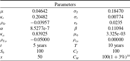
We fit a Nelson–Siegel model to the Belgian state yield curveFootnote 3 on the 23/11/22. Initial survival probabilities are described by a Makeham’s model adjusted to male Belgian mortality rates.Footnote 4 Details are provided in the Online Supplementary Materials. Other market parameters are estimated from time series of the Belgian stock index BEL 20 and of the 1 year Belgian state yield from the 26/11/10 to the 23/11/22. The correlations $\rho_{S\,\mu}$ and $\rho_{r\,\mu}$ are set to -5% and 0%. Parameter estimates are reported in Table 1.

Table 9.

Model parameters and features of the contract.

The three risk factors are the normed stock price, normed short rate, and normed mortality rate at the end of the time horizon of primary simulations, noted t:

\begin{align*}\boldsymbol{X}_{t} & :=\left(\frac{S_{t}-\mathbb{E}_{0}^{\mathbb{P}}\left(S_{t}\right)}{\sqrt{\mathbb{V}_{0}^{\mathbb{P}}\left(S_{t}\right)}},\frac{\sqrt{r_{t}}-\mathbb{E}_{0}^{\mathbb{P}}\left(r_{t}\right)}{\sqrt{\mathbb{V}_{0}^{\mathbb{P}}\left(\sqrt{r_{t}}\right)}},\frac{\sqrt{\mu_{x+t}}-\mathbb{E}_{0}^{\mathbb{P}}\left(\mu_{x+t}\right)}{\sqrt{\mathbb{V}_{0}^{\mathbb{P}}\left(\sqrt{\mu_{x+t}}\right)}}\right).\end{align*}

Expectations and variances are approached by empirical averages and variances of the simulated sample. The contract features are reported in Table 1. We simulate 10,000 primary scenarios and a single secondary response per scenario,

\begin{eqnarray*}Y(t) & = & e^{-\int_{t}^{T}r_{s}+\mu_{s}ds}\left(C_{T}+\left(S_{T}-C_{T}\right)_{+}-\left(S_{T}-C_{M}\right)_{+}\right).\end{eqnarray*}

We work with 350 steps of time per year. We also calculate the exact value of the contract in each scenario using the analytical formulas from previous section.

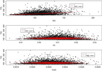
The plots of Figure 10 show responses versus stock prices, interest, and mortality rates. The red dots correspond to LSMC estimates of the endowment 1 year ahead, with a second-order polynomial of risk factors.

Figure 10.

Simulated responses $Y(t)=$ versus stock prices $S_{t}$ , $r_{t}$ and $\mu_{x}+t$ . The red dots are the predictions $h(\boldsymbol{X}_{t})$ from the LSMC with a second-order polynomials regression.

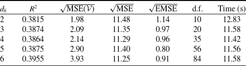
Table 10 reports the $R^{2}$ , the MSE, and MSE $(\mathcal{V})$ of the LSMC, such as defined by Equations (3.8), (3.10), and (3.11). The validation set counts 1000 triplets of risk factors. We consider combinations of $q=10$ empirical quantiles of risk factors for probabilities from 1 to 5% and from 95 to 99% by step of 1%. We also calculate the exact MSE between model and analytical prices of the endowment, denoted by EMSE.

Table 10.

$R^{2}$ , MSE, MSE $(\mathcal{V}),$ and runtimes of regressions of $Y_{t}$ on $\boldsymbol{X}_{t}$ in the LSMC model. $\sqrt{\text{EMSE}}$ is the MSE valued with analytical prices. d.f. is the number of parameters.

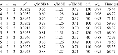
Table 10 provides statistics about LSMC polynomial regressions of order $d_{h}$ from 2 to 6. The $R^{2}$ s slightly increase with the complexity of the model. The MSE $(\mathcal{V})$ on the validation set is minimized by a polynomial of second degree. The LSMC is estimated in 12 s. Table 3 presents the statistics of goodness of fit for the LLSMC model. The number of clusters, K, varies from 2 to 5. We test polynomials of degrees $d_{h}$ from 1 to 3 and $d_{\gamma}$ equal to 1 and 3. Models are sorted by increasing MSE $(\mathcal{V})$ s and we report statistics of the 10 first best models according to this criterion. The optimal goodness of fit is achieved by using 5–3 clusters, a square or cubic regression on each cluster, and a cubic multinomial logistic regression. Compared to the LSMC, the LLSMC reduces the MSE $(\mathcal{V})$ and the EMSE by more than half, whereas MSE on the training set remains comparable. This indicates that the LLSMC model provides a better fit. The computational times range from 47 to 79 s depending on the model setting. We provide in the Online Supplementary Materials the goodness of fit statistics and runtimes for LSMC and LLSMC, computed with 100,000 simulations instead of 10,000. We do not observe significant differences in MSE and $R^{2}$ . This validates our choice to set the number of scenarios to 10,000.

Table 11.

$R^{2}$ , MSE, MSE $(\mathcal{V})$ , $R_{loc}^{2}$ , and runtimes for the LLSMC model. $\sqrt{\text{MSE}}$ , exact is the MSE valued with analytical prices. d.f. is the number of parameters.

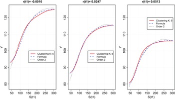
We next compare the LSMC of order 3 and the LLSMC with hyperparameters $K=5$ , $d_{\gamma}=3$ , $d_{h}=2$ as this setting leads to a low MSE $(\mathcal{V})$ and a high $R_{loc}^{2}$ . Figure 6 compares LSMC and LLSMC endowment values for stock prices $S_{t}$ ranging from 43 to 302, the 1% and 99% percentiles of simulated stock prices over 5 years and $r_{t}\in\{-0.16\%,2.47\%,5.13\%\}$ , and the 1%, 50%, and 99% quantiles of simulated interest rates. The mortality rate is set to its average $\mu_{x+t}=0.0017$ . LSMC and LLSMC both achieve a good accuracy in these three cases. Nevertheless, pricing errors of the LLSMC, reported in Table 12, are slightly lower on average than those of the LSMC when $r_{t}\in\{-0.16\%,2.47\%\}$ . In particular, the LLSMC better fits extremely low values. This will be confirmed by the comparison of VaRs and TVaRs.

Table 12.

Average pricing errors for the three cases presented in Figure 11.

Table 13.

VaR 5 years, LSMC model, and LLSMC.

Figure 11.

Endowment prices for $S_{t}$ ranging from 40 to 310, $r_{t}\in\{-0.16\%,2.47\%,5.13\%\}$ and $\mu_{x+t}=0.0017$ .

Figure 12.

Lower/upper VaRs and TVaRs, LLSMC 5-3-2, LSMC of order 3.

Table 14.

Expected shortfall, 5 years, LSMC model, and LLSMC.

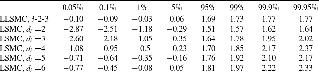
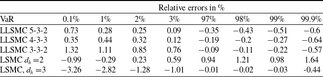
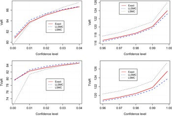
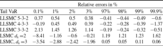
Figure 12 displays VaRs and TVaRs computed with the LLSMC 5-3-2, the LSMC of order 3, and analytical values. Tables 13 and 14 report the relative spread between VaR/TVaRs computed with approximated and exact analytical prices. These results emphasize that LLSMC provides a more accurate estimate of VaR/TVaRs. In particular, the LSMC’s inability to closely replicate extreme values results in a significant divergence of TVaR for very low or high confidence levels.