1. Introduction
The increasing demand for autonomous navigation across various sectors has brought tractor-trailer mobile robots (TTMRs) to the forefront of robotic research. These articulated mobile robots are commonly used in logistics, agriculture [Reference Lu, Zhao, Ma, Xu and Liu1, Reference Shojaei2], and industrial settings [Reference Zhao, Chen, Zhou, Zheng and Liu3], where transporting goods over long distances and maintaining maneuverability are essential [Reference Wang, Zhang and Wang4]. However, the complexity of these systems, including their nonholonomic constraints and kinematic coupling between the tractor and trailer units, presents unique challenges [Reference Shojaei and Abdolmaleki5]. In addition, achieving accurate trajectory tracking in environments where avoiding obstacles is critical adds another layer of complexity. Therefore, developing effective and safe control strategies remains an important area for further research.
Recent control strategies often treat trajectory tracking and obstacle avoidance as separate tasks, which can result in suboptimal performance in real-world scenarios. Some approaches focus on kinematic control [Reference Shojaei and Abdolmaleki5–Reference Kassaeiyan, Alipour and Tarvirdizadeh7], whereas others consider the dynamics and uncertainties in modeling [Reference Robat, Arezoo, Alipour and Tarvirdizadeh8, Reference Zhao, Zhou, Chen, Miao and Liu9]. Various methodologies have been investigated for precise trajectory tracking, including Model Predictive Control (MPC) [Reference Lukassek, Volz, Szabo and Graichen10, Reference Lukassek, Dahlmann, Völz and Graichen11], robust control [Reference Lu, Xue, Chen and Jiang12–Reference Zhou, Wen and Xu14], intelligent control [Reference Kumar15–Reference Ghasemzadeh, Amjadifard and Keymasi-Khalaji17], PID and Lyapunov-based control [Reference Khanpoor, Khalaji and Moosavian18], fuzzy control [Reference Elhaki and Shojaei19, Reference Yin, Wang, Gao and Li20], optimal control [Reference Nazemizadeh, Kolahi and Gandomkar21, Reference Rigatos, Busawon and Abbaszadeh22], and adaptive control [Reference Jin, Dai and Liang23, Reference Jin, Liang, Dai and Guo24]. In addition, researchers have added novel ideas for trajectory tracking. Such as backward motion [Reference Khalaji and Jalalnezhad25–Reference Bertolani, Bacheti, Brandão, Carelli and Sarcinelli-Filho28], addressing wheel slippage [Reference Alipour, Robat and Tarvirdizadeh29, Reference Khalaji and Jalalnezhad30], managing the control of multiple trailers [Reference Khalaji and Jalalnezhad31, Reference Deniz, Jorquera, Torres-Torriti and Cheein32], and handling actuator saturation [Reference Naderolasli, Shojaei and Chatraei33]. While all of these studies effectively address precise trajectory tracking, they often fall short when there are environmental constraints, such as static and dynamic obstacles, that the system must avoid. This limitation has paved the way for approaches that combine trajectory tracking and obstacle avoidance.
To the best of the authors’ knowledge, many studies have focused on trajectory planning algorithms for obstacle avoidance in long time-domain trajectory optimization [Reference Wang, Deng, Li, Wang, Jin and Su34, Reference Bitar, Martinsen, Lekkas and Breivik35], while only a few have addressed collision-free trajectory tracking for TTMR systems, highlighting a significant research gap in this field. In ref. [Reference Bushnell36], Bushnell presented an algorithm for planning obstacle avoidance paths for a car towing multiple trailers as one of the frontiers in the idea of obstacle avoidance trajectory tracking of TTMRs.
Several studies have employed MPC as the primary framework for trajectory tracking. For instance, in ref. [Reference Yue, Wu, Guo and Gao37], a quintic polynomial function was used to generate smooth obstacle avoidance trajectories, complemented by an MPC-based posture controller that ensured accurate trajectory tracking and enhanced robustness. Based on the lane-changing maneuvers scenario in this study, the lack of consideration of multiple obstacles and the presence of other vehicles can be observed. In ref. [Reference Murillo, Sánchez, Deniz, Genzelis and Giovanini38], a kinematic nonlinear model predictive controller (NMPC) was proposed to improve path-tracking performance in the presence of obstacles, particularly in precision agriculture applications. Although the study mentioned that obstacle avoidance could be incorporated into the controller, the simulations did not account for a collision-free trajectory tracking scenario. A more advanced nonlinear model predictive path-following controller (NMPPFC) in discrete-time format for the autonomous navigation of generalized N-trailer vehicles was presented in ref. [Reference Deniz and Cheein39]. This approach introduced a novel way to model obstacles as soft constraints using Gaussian functions, maintaining convexity, and ensuring computational efficiency compared with hard-constraint methods. In addition, the system combined a global path planner and a local path planner to handle path occlusion by obstacles, ensuring stability and feasibility. Moreover, a novel simultaneous planning and control (SPC) method proposed integrating an improved artificial potential field (IAPF) for robust, short-term trajectory planning with MPC for high-precision, real-time command generation, overcoming the limitations of traditional ”first planning then tracking” frameworks. The IAPF accounts for angular velocity constraints and provides time-based information, while the MPC handles dynamic constraints and external disturbances [Reference Wang, Liu, Peng, Qie, Zhao and Lu40].
Integrating discrete-time NMPC with control barrier functions (CBFs) has led to more robust control strategies for obstacle avoidance, particularly in dynamic environments like hospitals [Reference Tang, Mamaev, Qin, Wurll and Hein41]. Expanding on the concept of safety for autonomous TTMR systems, a multi-CBF framework combined with linear time-varying MPC (LTV-MPC) in discrete time was introduced in ref. [Reference Aali and Liu42]. This approach ensured collision-free maneuvers for both tractor and trailer in collision-free scenarios. Another noteworthy advancement is the integration of CBFs for safety guarantees with control Lyapunov functions (CLFs) for trajectory tracking, optimized through a quadratic program (QP). This method enabled safe and efficient trajectory tracking while avoiding obstacles during TTMR motions [Reference Cai, Wang, Zuo, Ji and Li43]. Despite these advances showing promising results in simulations and implementations, the trade-off between computational efficiency and control performance remains a critical challenge, guiding the direction of this research.
This study proposes a novel control approach that effectively combines efficient trajectory tracking with real-time obstacle avoidance. By utilizing inverse kinematics and pure integral control for closed-loop systems, a notably straightforward method, the kinematics of the robot are controlled effectively. Furthermore, when this approach is integrated with the dynamic controller of ref. [Reference Khalaji and Moosavian44] and simulated again, it demonstrates improved performance compared to the previous findings. This emphasizes the significant role of the kinematic controller in trajectory tracking.
To integrate obstacle avoidance mode (OAM) for trajectory tracking, two methods are explored. The first method is a customized APF acting on a kinematic controller, which has not been previously explored for trajectory tracking control of TTMR systems or any dynamical systems. In this method, two different approaches are used to test the effectiveness of the algorithms on large and small-scale case studies. The second method, which is a path planning method (PPM), was inspired by ref. [Reference Deniz and Cheein39] but has been tailored for continuous-time analysis, unlike the discrete-time planner proposed in that study. In our proposed method, when the robot reaches a predetermined radial distance from an obstacle, its last orientation is used to generate semi-circular or semi-elliptical trajectories, as a temporary reference. This not only enables the robot to navigate and avoid obstacles efficiently but also reverts to the primary reference trajectory smoothly. Further comparative analysis reveals that the most effective strategy for avoiding obstacles involves modifying the reference trajectory dynamically, rather than relying solely on angular corrections managed by the controller in the APF methods.
The main contributions of this work include: 1) development and implementation of a computationally efficient control framework that seamlessly integrates trajectory tracking and collision avoidance, 2) development of a novel path planning method in a continuous-time format to avoid obstacles in the reference trajectory, and 3) comprehensive validation of the proposed approach through simulation for safe operation across various trajectories.
The work is organized as follows. Section 2 details the configuration of the TTMR system, covering its kinematic and dynamic models. Section 3 presents the controller design, including the kinematic and dynamic control strategies. Section 4 discusses methods for collision-free trajectory tracking in static and dynamic environments, incorporating artificial potential field techniques and the PPM. Section 5 provides simulation results that validate the performance of the proposed methods in diverse scenarios. Finally, as the conclusion, the contributions and future research directions are outlined.
Schematic representation of the tractor-trailer system.

2. TTMR system configuration
The TTMR system comprises a tractor and trailer connected via a revolute joint at point
 $P_0$
. Figure 1 illustrates the system model. The distance between points
 $P_0$
and
 $P_1$
is denoted by
 $d$
. The centroids of the tractor and trailer are labeled as
 $C_0$
and
 $C_1$
, respectively, with distances
 $a_0$
and
 $a_1$
measured between
 $P_0, C_0$
and
 $P_1, C_1$
.
 $\varphi _l$
and
 $\varphi _r$
represent the angular displacements of the left and right wheels,
 $r$
is the radius of the wheels, and
 $b_0 = b_1$
is the half of the distance between the tractor and the trailer. Furthermore, the following assumptions are used to create a simplified model: (1) the trailer is attached to the tractor by a rigid linkage; (2) the wheels operate under conditions of pure rolling, without any lateral or longitudinal slipping; (3) the articulated connection permits only rotational motion around the pivot; (4) the robot under consideration is TTMR with an on-axle hitching; (5) the tractor’s wheels are actuated, while the trailer’s wheels are passive. A global coordinate system
 $(X,Y)$
serves as the inertial frame of reference. The configuration vector of the system is defined as
 $\boldsymbol{\eta } = [x, y, \theta _1, \theta _0]^T$
, where
 $(x, y)$
represents the position of the point
 $P_1$
(the midpoint between the wheels of the trailer) in the inertial frame, and
 $\theta _0$
and
 $\theta _1$
are the angular positions of the tractor and trailer, respectively. The deviation of the trailer position from the reference trajectory is denoted by
 $e$
, which quantifies the tracking error. For clarity, the nomenclature of all symbols and parameters employed in this study is summarized in Appendix Table AI.
2.1. System kinematics
The kinematics of the system can be expressed as
 \begin{equation} \dot {\boldsymbol{\eta }} = \begin{bmatrix} \cos (\theta _1) &\quad 0 \\ \sin (\theta _1) &\quad 0 \\ \tan (\psi )/d &\quad 0 \\ 0 &\quad 1 \end{bmatrix} \begin{bmatrix} v_1 \\ v_2 \end{bmatrix} = S(\boldsymbol{\eta }) \, \boldsymbol{v} \end{equation}
where
 $S(\boldsymbol{\eta })$
is the kinematic matrix,
 $\psi = \theta _0 - \theta _1$
is the difference between tractor and trailer heading angles, and
 $\boldsymbol{v}$
contains the linear (
 $v_1$
) and angular velocities (
 $v_2$
) of the trailer, in which
 $v_1 = \frac {r}{2} \dot {\varphi }^+ \cos (\psi ), v_2 = \frac {r}{2b_0} \dot {\varphi }^-$
. (Note that
 $\dot {\varphi }^+ = \dot {\varphi }_r + \dot {\varphi }_l$
and
 $\dot {\varphi }^- = \dot {\varphi }_r - \dot {\varphi }_l$
.)
Remark 1: It is important to note that the kinematic model is derived by considering the matrix representation of the nonholonomic constraints on the motion of the TTMR system, as seen in (2). The results of the matrix calculations indicate that the first row corresponds to the constraints on the trailer, while the second row pertains to the tractor. Considering the system constraint matrix
 $\mathcal{A}(\boldsymbol{\eta })$
and the kinematic matrix, it shows that they satisfy natural orthogonality,
 $S^T(\boldsymbol{\eta })\mathcal{A}^T(\boldsymbol{\eta }) = 0$
.
 \begin{equation} \underbrace { \begin{bmatrix} \sin (\theta _0) &\quad -\cos (\theta _0) &\quad -d \cos (\psi ) &\quad 0 \\ \sin (\theta _1) &\quad -\cos (\theta _1) &\quad 0 &\quad 0 \end{bmatrix} }_{\mathcal{A}(\boldsymbol{\eta })} \begin{bmatrix} \dot {x} \\ \dot {y} \\ \dot {\theta }_1 \\ \dot {\theta }_0 \end{bmatrix} = 0 \quad \Rightarrow \quad \mathcal{A}(\boldsymbol{\eta }) \dot {\boldsymbol{\eta }} = 0 \end{equation}
2.2. System dynamics
The dynamics of the TTMR are described by (3), where
 $M(\boldsymbol{\eta })$
,
 $B(\boldsymbol{\eta })$
,
 $C(\boldsymbol{\eta }, \dot {\boldsymbol{\eta }})$
, and
 $\mathcal{A}(\boldsymbol{\eta })$
are system matrices,
 $\boldsymbol{\lambda }$
represents the vector of Lagrange multipliers, and
 $\boldsymbol{\tau }$
is the vector of actuator forces and torques. To be specific in the formulation,
 $M(\boldsymbol{\eta })$
is the mass matrix of the system,
 $C(\boldsymbol{\eta }, \dot {\boldsymbol{\eta }})$
captures the Coriolis and centrifugal effects,
 $\mathcal{A}^T(\boldsymbol{\eta }) \boldsymbol{\lambda }$
represents the constraint forces applied to the wheels, and
 $B(\boldsymbol{\eta }) \boldsymbol{\tau }$
corresponds to actuator inputs. The matrix representations of each are specified in (4).
 \begin{equation} M(\boldsymbol{\eta }) \ddot {\boldsymbol{\eta }} + C(\boldsymbol{\eta }, \dot {\boldsymbol{\eta }}) \dot {\boldsymbol{\eta }} = B(\boldsymbol{\eta }) \boldsymbol{\tau } + \mathcal{A}^T(\boldsymbol{\eta }) \boldsymbol{\lambda } \end{equation}
 \begin{equation} \begin{aligned} M(\boldsymbol{\eta }) &= \begin{bmatrix} M &\quad 0 &\quad -A \sin (\theta _1) &\quad a_0 m_0 \sin (\theta _0) \\ 0 &\quad M &\quad A \cos (\theta _1) &\quad a_0 m_0 \cos (\theta _0) \\ -A \sin (\theta _1) &\quad A \cos (\theta _1) &\quad I_{\theta _1} &\quad 0 \\ a_0 m_0 \sin (\theta _0) &\quad a_0 m_0 \cos (\theta _0) &\quad 0 &\quad I_{\theta _0} \end{bmatrix}, \\[10pt] B(\boldsymbol{\eta }) &= \frac {1}{r} \begin{bmatrix} \cos (\theta _0) &\quad \cos (\theta _0) \\ \sin (\theta _0) &\quad \sin (\theta _0) \\ d \sin (\psi ) &\quad d \sin (\psi ) \\ b &\quad -b \end{bmatrix}, \quad C(\boldsymbol{\eta }, \dot {\boldsymbol{\eta }}) = \begin{bmatrix} -a_0 m_0 \cos (\theta _0) \dot {\theta }_0^2 - A \cos (\theta _1) \dot {\theta }_1^2 \\[3pt] -a_0 m_0 \sin (\theta _0) \dot {\theta }_0^2 - A \sin (\theta _1) \dot {\theta }_1^2 \\[3pt] -a_0 d m_0 \dot {\theta }_0^2 \sin (\psi ) \\[3pt] a_0 d m_0 \dot {\theta }_1^2 \sin (\psi ) \end{bmatrix} \end{aligned} \end{equation}
where
 $M = m_0 + m_1$
,
 $A = a_1 m_1 + d m_0$
,
 $I_{\theta _1} = m_1 a_1^2 + m_0 d^2 + I_1$
,
 $I_{\theta _0} = m_0 a_0^2 + I_0$
, and
 $\boldsymbol{\tau } = [\tau _r, \tau _l]^T$
.
Considering that superscript
 $0$
is used for the tractor and superscript
 $1$
for trailer,
 $m_0$
and
 $m_1$
are the mass of TTMR,
 $a_0$
and
 $a_1$
are used to represent the distance between COM and midpoints of TTMR,
 $I_{0}$
and
 $I_{1}$
are their mass moments of inertia about the vertical axis. In addition,
 $I_{\theta _0}$
and
 $I_{\theta _1}$
are the moments of inertia.
By differentiating kinematic equation (1), the acceleration of the system can be expressed as
 \begin{equation} \ddot {\boldsymbol{\eta }} = S(\boldsymbol{\eta }) \dot {\boldsymbol{v}} + \dot {S}(\boldsymbol{\eta }) \boldsymbol{v} \end{equation}
Substituting (1) and (5) into dynamic equation (3), the system dynamics can be reformulated as:
 \begin{equation} M_1(\boldsymbol{\eta }) \dot {\boldsymbol{v}} + M_2(\boldsymbol{\eta }) \boldsymbol{v} + C_1(\boldsymbol{\eta }, \dot {\boldsymbol{\eta }}) = B_1(\boldsymbol{\eta }) \boldsymbol{\tau } \end{equation}
where
 $M_1(\boldsymbol{\eta }) = S(\boldsymbol{\eta })^T M(\boldsymbol{\eta }) S(\boldsymbol{\eta })$
,
 $M_2(\boldsymbol{\eta }) = S(\boldsymbol{\eta })^T M(\boldsymbol{\eta }) \dot {S}(\boldsymbol{\eta })$
,
 $C_1(\boldsymbol{\eta }, \dot {\boldsymbol{\eta }}) = S(\boldsymbol{\eta })^T C(\boldsymbol{\eta }, \dot {\boldsymbol{\eta }})$
, and
 $B_1(\boldsymbol{\eta }) = S(\boldsymbol{\eta })^T B(\boldsymbol{\eta })$
.
Finally, the mathematical representation of torque is shown in (7), and for the sake of simplicity, its revised version is shown in (8), where
 $M_3(\boldsymbol{\eta }) = B_1^{-1}(\boldsymbol{\eta }) M_1(\boldsymbol{\eta }), M_4(\boldsymbol{\eta }) = B_1^{-1}(\boldsymbol{\eta }) M_2(\boldsymbol{\eta }), C_2(\boldsymbol{\eta }, \dot {\boldsymbol{\eta }}) = B_1^{-1}(\boldsymbol{\eta }) C_1(\boldsymbol{\eta }, \dot {\boldsymbol{\eta }})$
.
 \begin{equation} \boldsymbol{\tau } = B_1^{-1}(\boldsymbol{\eta }) \left [ M_1(\boldsymbol{\eta }) \dot {\boldsymbol{v}} + M_2(\boldsymbol{\eta }) \boldsymbol{v} + C_1(\boldsymbol{\eta }, \dot {\boldsymbol{\eta }}) \right ] \end{equation}
 \begin{equation} \boldsymbol{\tau } = M_3(\boldsymbol{\eta }) \dot {\boldsymbol{v}} + M_4(\boldsymbol{\eta }) \boldsymbol{v} + C_2(\boldsymbol{\eta }, \dot {\boldsymbol{\eta }}) \end{equation}
3. Controller design
This section presents the proposed controller based on the inverse kinematics of a TTMR in addition to pure integral controllers for trajectory tracking control. Utilizing the dynamic controller of ref. [Reference Khalaji and Moosavian44] demonstrates a significant improvement compared to previous studies, as detailed later in Section 5. After designing the controller for trajectory tracking, the concept of obstacle avoidance in complex environments using three different approaches is discussed.
3.1. Kinematic control unit
For designing the kinematic controller, states of the system (
 $\boldsymbol{\eta } = [x, y, \theta _1, \theta _0]^T$
) and their derivatives (
 $\dot {\boldsymbol{\eta }} = [\dot {x}, \dot {y}, \dot {\theta }_1, \dot {\theta }_0]^T$
) are required. Because the approach is to track the reference trajectory, its states and derivatives should also be defined in (9) and (10).
 \begin{equation} \boldsymbol{\eta }_r = [x_r, y_r, \theta _{1r}, \theta _{0r}]^T = [{\eta }_{1r}, {\eta }_{2r}, {\eta }_{3r}, {\eta }_{4r}]^T \end{equation}
 \begin{equation} \dot {\boldsymbol{\eta }}_r = [\dot {x}_r, \dot {y}_r, \dot {\theta }_{1r}, \dot {\theta }_{0r}]^T = [\dot {\eta }_{1r}, \dot {\eta }_{2r}, \dot {\eta }_{3r}, \dot {\eta }_{4r}]^T \end{equation}
As previously mentioned, the main focus of this study is to control the robot using the inverse kinematics approach. In this regard, the reference kinematic (11) should first be formulated based on the reference states (9) and (10), where
 $\psi _r = \theta _{0r} - \theta _{1r}$
. Using the pseudoinverse of the reference motion matrix (
 $S_r^\dagger (\boldsymbol{\eta }_r)$
), the control input (
 $\boldsymbol{v}_r$
) for the open-loop system will be like (12). Replacing the updated version of
 $\boldsymbol{v}_r$
as the kinematic control law into the original kinematic mathematical representation of the TTMR system (1) yields (13).
 \begin{equation} \dot {\boldsymbol{\eta }}_r = \begin{bmatrix} \cos (\theta _{1r}) &\quad 0 \\ \sin (\theta _{1r}) &\quad 0 \\ \tan (\psi _r)/d &\quad 0 \\ 0 &\quad 1 \end{bmatrix} \boldsymbol{v}_r = S_r(\boldsymbol{\eta }_r)\boldsymbol{v}_r \end{equation}
 \begin{equation} \boldsymbol{v}_r = S_r^\dagger (\boldsymbol{\eta }_r) \dot {\boldsymbol{\eta }}_r \end{equation}
 \begin{equation} \dot {\boldsymbol{\eta }} = S(\boldsymbol{\eta }) \boldsymbol{v}_r \quad \Rightarrow \quad \dot {\boldsymbol{\eta }} = S(\boldsymbol{\eta }) S_r^\dagger (\boldsymbol{\eta }_r) \dot {\boldsymbol{\eta }}_r \quad \Rightarrow \quad \dot {\boldsymbol{\eta }} \cong I_{4 \times 4} \dot {\boldsymbol{\eta }}_r \end{equation}
Remark 2: Here,
 $S_r^\dagger (\boldsymbol{\eta }_r)$
acts like a pre-compensator matrix, used for making its product with
 $S(\boldsymbol{\eta })$
equal to a
 $4 \times 4$
identity matrix. Note that this property is valid when the initial positions of the robot and the reference are the same, that is,
 $\boldsymbol{\eta } = \boldsymbol{\eta }_r$
. Due to the fact that the robot may have some distance from the reference path, the result of this product (
 $S(\boldsymbol{\eta }) S_r^\dagger (\boldsymbol{\eta }_r)$
) may not be an identity matrix, but it is a near-diagonal matrix that is very similar to identity, which is sufficient for control purposes. The detailed calculations are given in the following.
 \begin{equation} S(\boldsymbol{\eta }) S_r^\dagger (\boldsymbol{\eta }_r) = \begin{bmatrix} \cos (\theta _1) &\quad 0 \\ \sin (\theta _1) &\quad 0 \\ \tan (\psi _r)/d &\quad 0 \\ 0 &\quad 1 \end{bmatrix} \begin{bmatrix} \displaystyle\frac {\cos (\theta _{1r})}{1 + \frac {\tan ^2(\psi _r)}{d^2}} &\quad \displaystyle\frac {\sin (\theta _{1r})}{1 + \frac {\tan ^2(\psi _r)}{d^2}} &\quad \displaystyle\frac {\tan (\psi _r)/d}{1 + \frac {\tan ^2(\psi _r)}{d^2}} &\quad 0 \\[12pt] 0 &\quad 0 &\quad 0 &\quad 1 \end{bmatrix} \end{equation}
 \begin{equation} S(\boldsymbol{\eta }) S_r^\dagger (\boldsymbol{\eta }_r) = \begin{bmatrix} \displaystyle\frac {\cos (\theta _1) \cos (\theta _{1r})}{1 + \frac {\tan ^2(\psi _r)}{d^2}} &\quad \displaystyle\frac {\cos (\theta _1) \sin (\theta _{1r})}{1 + \frac {\tan ^2(\psi _r)}{d^2}} &\quad \displaystyle\frac {\cos (\theta _1)\tan (\psi _r)/d}{1 + \frac {\tan ^2(\psi _r)}{d^2}} &\quad 0 \\[13pt] \displaystyle\frac {\sin (\theta _1) \cos (\theta _{1r})}{1 + \frac {\tan ^2(\psi _r)}{d^2}} &\quad \displaystyle\frac {\sin (\theta _1) \sin (\theta _{1r})}{1 + \frac {\tan ^2(\psi _r)}{d^2}} &\quad \displaystyle\frac {\sin (\theta _1)\tan (\psi _r)/d}{1 + \frac {\tan ^2(\psi _r)}{d^2}} &\quad 0 \\[13pt] \displaystyle\frac {\tan (\psi _r)/d \cos (\theta _{1r})}{1 + \frac {\tan ^2(\psi _r)}{d^2}} &\quad \displaystyle\frac {\tan (\psi _r)/d \sin (\theta _{1r})}{1 + \frac {\tan ^2(\psi _r)}{d^2}} &\quad \displaystyle\frac {\tan ^2(\psi _r)/d^2}{1 + \frac {\tan ^2(\psi _r)}{d^2}} &\quad 0 \\[12pt] 0 &\quad 0 &\quad 0 &\quad 1 \end{bmatrix} \end{equation}
From (15), it can be said that the product
 $S(\boldsymbol{\eta }) S_r^\dagger (\boldsymbol{\eta }_r)$
has the following structure:
 \begin{equation} S(\boldsymbol{\eta }) S_r^\dagger (\boldsymbol{\eta }_r) = \begin{bmatrix} \text{(near 1)} &\quad \text{(small values)} &\quad \text{(small values)} &\quad 0 \\ \text{(small values)} &\quad \text{(near 1)} &\quad \text{(small values)} &\quad 0 \\ \text{(small values)} &\quad \text{(small values)} &\quad \text{(near 1)} &\quad 0 \\ 0 &\quad 0 &\quad 0 &\quad 1 \end{bmatrix} = \begin{bmatrix} s_{11} &\quad s_{12} &\quad s_{13} &\quad s_{14} \\ s_{21} &\quad s_{22} &\quad s_{23} &\quad 0 \\ s_{31} &\quad s_{32} &\quad s_{33} &\quad 0 \\ 0 &\quad 0 &\quad 0 &\quad 1 \end{bmatrix} \end{equation}
It is evident that the diagonal values of the first three rows/columns (
 $s_{11}, s_{22}, s_{33}$
) are close to 1 but not exactly 1 due to the term
 $1 + \frac {\tan ^2(\psi _r)}{d^2}$
in the denominator. However, the off-diagonal values are small, making the matrix nearly diagonal.
Kinematic control diagram of the system (integration of light-red blocks configures the closed-loop kinematic control).

The proposed algorithm, depicted in Figure 2, with blue blocks, is used for open-loop control purposes. As shown, the inputs to the pre-compensator matrix, consists of
 $[\dot {\eta }_{1r}, \dot {\eta }_{2r}, {\eta }_{3r}, \dot {\eta }_{3r}, {\eta }_{4r}, \dot {\eta }_{4r}]^T$
and denoted as [IN
 $_1$
, IN
 $_2$
, IN
 $_3$
, IN
 $_4$
, IN
 $_5$
, IN
 $_6$
]
 $^T$
. This input matrix combines the derivatives of the reference states and the reference orientation states, as mentioned above in (9) and (10).
To precisely control the position of the robot to be near the desired trajectory, which makes the near-diagonal matrix equal to identity, the control loop should be closed as denoted by light-red blocks and feedbacks in Figure 2. As shown in the Figure 2, three integral controllers for each state are added to the control loop to help the pre-compensator matrix (inverse kinematics), depicted by the mux block, make the states of the robot converge to its desired values. In the closed-loop format, the inputs of the pre-compensator block are
 $[\dot {\boldsymbol{\eta }}_{1r_{CL}}, \dot {\boldsymbol{\eta }}_{2r_{CL}}, {\boldsymbol{\eta }}_{3r_{CL}},\dot {\boldsymbol{\eta }}_{3r_{CL}},{\boldsymbol{\eta }}_{4r_{CL}},\dot {\boldsymbol{\eta }}_{4r_{CL}}]^T$
, as defined in the right hand side matrix of (17). Finally, the closed-loop kinematic control law is given in (17), where
 $e_x = {\eta }_{1r} - \eta _1$
,
 $e_y = {\eta }_{2r} - \eta _2$
, and
 $e_{\theta _1} = {\eta }_{3r} - \eta _3$
.
 \begin{equation} \boldsymbol{v} = S_r^\dagger (\boldsymbol{\eta }_{rCL}) \begin{bmatrix} \dot {\eta }_{1rCL} \\ \dot {\eta }_{2rCL} \\ \dot {\eta }_{3rCL} \\ \dot {\eta }_{4rCL} \end{bmatrix} = S_r^\dagger (\boldsymbol{\eta }_{rCL}) \begin{bmatrix} k_1 e_x \\ k_2 e_y \\ k_3 e_{\theta _1} \\ \dot {\theta }_{0r} \end{bmatrix} \end{equation}
3.1.1. Stability analysis
Steady-state error for each control loop is evaluated in (18)–(20). In real-world applications, this near-identity structure is sufficient to ensure the stability of numerical computations or control systems. By closing the loop, the integral controller can effectively handle the small values of (16), considering them as very low disturbances owing to the robust characteristics of the controller. Furthermore, similar to linear systems, the stability of the closed-loop system can be demonstrated as follows.
 \begin{equation} e_x(\infty ) = \lim _{s \to 0} \frac {s \cdot x_r}{1 + \frac {k_1}{s} \cdot s_{11}} = \lim _{s \to 0} \frac {s \cdot (0.01s + 1) \cdot x_r}{0.01s + 1 + k_1} \cong 0 \end{equation}
 \begin{equation} e_y(\infty ) = \lim _{s \to 0} \frac {s \cdot y_r}{1 + \frac {k_2}{s} \cdot s_{22}} = \lim _{s \to 0} \frac {s \cdot (0.01s + 1) \cdot y_r}{0.01s + 1 + k_2} \cong 0 \end{equation}
 \begin{equation} e_{\theta _1}(\infty ) = \lim _{s \to 0} \frac {s \cdot \theta _{1r}}{1 + \frac {k_3}{s} \cdot s_{33}} = \lim _{s \to 0} \frac {s \cdot (0.01s + 1) \cdot \theta _{1r}}{0.01s + 1 + k_3} \cong 0 \end{equation}
Remark 3: Since the steady-state error
 $x, y, \theta _1$
is zero, we have
 $x \to x_r$
,
 $y \to y_r$
,
 $\theta _1 \to \theta _{1r}$
,
 $\dot {\theta }_1 \to \dot {\theta }_{1r}$
. Based on the reason that
 $\theta _0$
is dependent on bounded states of the trailer, the steady-state error of
 $\theta _0$
(21) and its derivative also converge to zero. As a result,
 $\theta _0 \to \theta _{0r}$
,
 $\dot {\theta }_0 \to \dot {\theta }_{0r}$
. Therefore, in this control method, only three closed loops are required for four states.
 \begin{equation} e_{\theta _0} = \theta _{0r} - \theta _0 = \theta _{1r} + \text{atan2} \left ( \frac {L \times \dot {\theta }_{1r} \sqrt {\dot {x}_r^2 + \dot {y}_r^2}}{\dot {\theta }_{0r}} \right ) - \theta _1 + \text{atan2} \left ( \frac {L \times \dot {\theta }_1 \sqrt {\dot {x}^2 + \dot {y}^2}}{\dot {\theta }_0} \right ) \end{equation}
3.2. Dynamic control unit
Based on the velocity tracking error, the dynamic control law for actuator torques is designed in the following. The tracking error signal is defined as
 $\boldsymbol{\xi } = \boldsymbol{v}_d - \boldsymbol{v}$
, where
 $\boldsymbol{v}_d$
is the desired velocity command signal obtained from the kinematic control law. Evidently, when the tracking error converges to zero, the system velocity follows the desired command. The control law is formulated as in (22), where
 $\mathcal{K} = \text{diag}(\mathcal{K}_1, \mathcal{K}_2)$
is a diagonal matrix with positive gains [Reference Khalaji and Moosavian44].
 \begin{equation} \boldsymbol{\tau } = M_3(\boldsymbol{\eta }) \dot {\boldsymbol{v}}_d + M_4(\boldsymbol{\eta }) \boldsymbol{v} + C_2(\boldsymbol{\eta }, \dot {\boldsymbol{\eta }}) + M_3(\boldsymbol{\eta }) \mathcal{K} \boldsymbol{\xi } \end{equation}
Property 1. It can be verified that the tracking errors converge to zero. Using the Lyapunov candidate function and its derivative with respect to time in (23) and (24), respectively:
 \begin{equation} V_1 = \frac {1}{2} \boldsymbol{\xi }^T \boldsymbol{\xi } \end{equation}
 \begin{equation} \dot {V}_1 = \boldsymbol{\xi }^T \dot {\boldsymbol{\xi }} = \boldsymbol{\xi }^T (\dot {\boldsymbol{v}}_d - \dot {\boldsymbol{v}}) \end{equation}
Using the torque formulation in (7) to update
 $\dot {V}_1$
and applying simplifications, we get:
 \begin{equation} \dot {V}_1 = \boldsymbol{\xi }^T \left [ \dot {\boldsymbol{v}}_d - M_3^{-1}(\boldsymbol{\eta }) \left \{ \boldsymbol{\tau } - M_4(\boldsymbol{\eta }) \boldsymbol{v} - C_2(\boldsymbol{\eta }, \dot {\boldsymbol{\eta }}) \right \} \right ] \end{equation}
 \begin{equation} \dot {V}_1 = - \boldsymbol{\xi }^T \mathcal{K} \boldsymbol{\xi } \end{equation}
Since
 $\dot {V}_1$
is negative definite, the Lyapunov stability criterion guarantees that the TTMR’s velocity will asymptotically follow the desired command signals [Reference Khalaji and Moosavian44].
4. Collision-free trajectory tracking control in complex environments
Collision-free motion tracking control in complex environments involves guiding a robot from an initial position to a target destination along a desired trajectory, defined by time parameters, while avoiding collisions with stationary and dynamic obstacles. For tractor-trailer systems, this task is particularly complex due to their nonholonomic constraints and the dynamic interactions between the tractor and trailer. This section examines the use of two variations of the APF method and introduces a novel PPM designed to enhance trajectory tracking in OAM.
In the APF approach, an obstacle avoidance signal is computed and integrated into the heading angle of the kinematic controller. Alternatively, in the PPM, when the robot approaches a predetermined distance from an obstacle, its most recent orientation is used to generate semi-circular or semi-elliptical trajectories as a temporary reference. This method not only facilitates efficient obstacle avoidance but also ensures a smooth return to the primary reference trajectory, enabling seamless navigation.
4.1. Artificial potential field method
This method employs gravitational and repulsion fields to affect the robot as interactive forces to ensure obstacle avoidance. Specifically, the virtual repulsive force is considered to steer the robot away from obstacles, while the gravitational force is assumed to guide the robot toward its target. Inspired by the methodology presented in ref. [Reference Liu, Chen, Liu, Zhang, Wu and Liu45], obstacles are modeled as circles with the radii of
 $R_{on}$
based on their outermost points, adding a layer of realism and flexibility for irregular shapes. Moreover, two extra concentric boundaries around each obstacle are introduced, which is the key innovation of this APF method, to enhance safety in obstacle avoidance and tracking.
Obstacle modeling in the proposed APF method, featuring concentric safety boundaries and the OAM region.

The inner boundary is set with a margin nearly equal to half the total length of the robot and its tractor (
 $b_r = L/2$
). This represents the minimum safe radius, meaning robots should not enter this zone under any circumstances. Meanwhile, the outer boundary (
 $b_s$
) accounts for errors and uncertainties that could affect the robot’s motion. This configuration is shown in Figure 3. A notable aspect of this virtual potential field method is its conditional activation. The repulsive force becomes effective only when the robot is within the bounds of OAM (
 $b_{OAM} = b_r + b_s$
). Outside this region, the robot controller focuses exclusively on path tracking. In real-world terms, this mechanism can be likened to a sensor on a robot that detects a predefined distance from an obstacle. Upon detection, the sensor sends a signal to activate the obstacle avoidance segment. Because the primary objective of this study is path tracking rather than waypoint tracking, the goal point should be considered in a way that can be adapted to a path-tracking context. To achieve this, the furthest intersection (relative to the robot) of the outermost obstacle boundary with the reference path is designated as the goal point [Reference Mao, Wu and You46] (
 $P_G$
in Figure 3). This idea aligns seamlessly with the essence of path tracking: when the robot deviates from the main path, it is guided back to the closest point on the desired trajectory.
In this method, two approaches are implemented: the first computes a cumulative force vector, and the second decomposes the forces into longitudinal and lateral components. The differences in how these forces are computed lead to variations in the precision of the robot’s heading angle adjustments, depending on the size of the map. These two approaches, discussed in the following subsections, are unique in the literature as they apply these principles to the TTMR and its kinematics, enhancing both simplicity and computational efficiency.
4.1.1. First approach: artificial potential field 1
The gravitational potential function for the
 $n^{\text{th}}$
goal is located at
 $P_{Gn} = (x_{Gn}, y_{Gn})$
and is given by (27), where
 $K_{Gn}$
is the design positive gain, and
 $\vec {r}_{Gn}$
(28) is the distance vector between the center of the
 $n^{\text{th}}$
goal and the position of the trailer robot at point
 $P_r = (x, y)$
, that is, the distance between
 $P_{Gn}$
and
 $P_r$
. The negative gradient of the gravitational potential function yields the corresponding gravitational force, depicted in (29).
 \begin{equation} U_{Gn} = \frac {1}{2} K_{Gn} \| \vec {r}_{Gn} \|^2 \end{equation}
 \begin{equation} \vec {r}_{Gn} = (x_{Gn} - x)\,\hat {\imath } + (y_{Gn} - y)\,\hat {\jmath } \quad \Rightarrow \quad \| \vec {r}_{Gn} \| = \sqrt {(x_{Gn} - x)^2 + (y_{Gn} - y)^2} \end{equation}
 \begin{equation} \vec {F}_{Gn} = -\nabla U_{Gn} = K_{G}^2 \vec {r}_{Gn} \end{equation}
On the other hand, consider the repulsion field function as in (30), where
 $K_{re}$
is the design positive gain, and
 $r_{on}$
(31) is the distance between the center of the
 $n^{\text{th}}$
obstacle at
 $P_{on} = (x_{on}, y_{on})$
and
 $P_r$
. The negative gradient of the repulsion potential function yields the corresponding repulsive force as depicted in (32).
 \begin{equation} U_{ren} = \begin{cases} \frac {1}{2} K_{re} \left ( \frac {1}{r_{on}} - \frac {1}{R_{OM}} \right )^2 \| \vec {r}_{Gn} \|^2, & 0 \leq r_{on} \leq b_{OM} \\ 0, & r_{on} \gt b_{OM} \end{cases} \end{equation}
 \begin{equation} r_{on} = \sqrt {(x_{on} - x)^2 + (y_{on} - y)^2} \end{equation}
 \begin{equation} \vec {F}_{ren} = -\nabla U_{ren} = \begin{cases} K_{re} \left ( \frac {1}{r_{on}} - \frac {1}{R_{OM}} \right ) \frac {\vec {r}_{Gn}}{r_{on}^2} \| \vec {r}_{Gn} \|^2 + K_{re} \left ( \frac {1}{r_{on}} - \frac {1}{R_{OM}} \right ) \vec {r}_{Gn}, & 0 \leq r_{on} \leq b_{OM} \\ 0, & r_{on} \gt b_{OM} \end{cases} \end{equation}
Thus, the cumulative force vector, including gravitational and repulsive components, acting on the TTMR is shown in (33). The desired control angle
 $\alpha _{OM}$
, calculated in (34), should be added to the original heading angle of the robot when entering the OAM mode, as described in 4.1.3
 \begin{equation} \vec {F} = \vec {F}_G(\vec {r}_G) + \sum _{j=1}^{n} \vec {F}_{re}^{(j)}(r_o) \end{equation}
 \begin{equation} \alpha _{OM} = \angle \vec {F} \vec {r}_{0n} \end{equation}
4.1.2. Second approach: artificial potential field 2
In the second approach, similar to the concepts of ref. [Reference Shi and Zhao47], the repulsive and gravitational forces are divided in longitudinal and lateral coordinates (
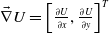 $\vec {\nabla }U = \left [\frac {\partial U}{\partial x}, \frac {\partial U}{\partial y} \right ]^T$
). The gravitational field expression remains the same as in (35) and (36), with the corresponding force shown in (37), where
 $\vec {F}_{Gx} = -\frac {\partial U_{Gn}}{\partial x}$
and
 $\vec {F}_{Gy} = -\frac {\partial U_{Gn}}{\partial y}$
.
 \begin{equation} U_{Gn} = \frac {1}{2} K_{Gn} \| \vec {r}_{Gn} \|^2 \end{equation}
 \begin{equation} \| \vec {r}_{Gn} \| = \sqrt {(x_{Gn} - x)^2 + (y_{Gn} - y)^2} \end{equation}
 \begin{equation} \vec {F}_{Gn} = -\nabla U_{Gn} = \begin{Bmatrix} K_{Gn}(x_{Gn} - x) = F_{Gnx} \\ K_{Gn}(y_{Gn} - y) = F_{Gny} \end{Bmatrix} \end{equation}
Similarly, the repulsion field function
 $U_{ren}$
and robot’s distance to the
 $n^{\text{th}}$
obstacle
 $r_{on}$
follow (30) and (31), but their gradients are calculated component-wise as shown in (38), where
 $F_{onx} = -\frac {\partial U_{ren}}{\partial x}$
and
 $F_{ony} = -\frac {\partial U_{ren}}{\partial y}$
.
 \begin{equation} \vec {F}_{ren} = -\nabla U_{ren} = \begin{Bmatrix} \displaystyle F_{onx} = K_{on}(x - x_{on}) \left ( \frac {1}{R_{OM}} - \frac {1}{r_{on}} \right )^2 + K_{on}(x - x_{on}) \left ( \frac {1}{R_{OM} \cdot r_{on}^2} \right ) \| \vec {r}_{Gn} \|^2 \\[10pt] \displaystyle F_{ony} = K_{on}(y - y_{on}) \left ( \frac {1}{R_{OM}} - \frac {1}{r_{on}} \right )^2 + K_{on}(y - y_{on}) \left ( \frac {1}{R_{OM} \cdot r_{on}^2} \right ) \| \vec {r}_{Gn} \|^2 \end{Bmatrix} \end{equation}
Thus, the cumulative force vector is:
 \begin{equation} \vec {F} = \vec {F}_x + \vec {F}_y = \begin{Bmatrix} F_{rx} = F_{Gnx} + F_{onx} \\ F_{ry} = F_{Gny} + F_{ony} \end{Bmatrix} \end{equation}
 \begin{equation} \alpha _{OM} = \tan ^{-1}\left ( \frac {F_{ry}}{F_{rx}} \right ) \end{equation}
4.1.3. Motion control law in complex environment
Building upon the APF method, the corresponding adjustment
 $\alpha _{OM}$
(in (34) and (40)) must be integrated into the motion control laws. Consequently, the control inputs from Figure 2 are modified as follows:
 \begin{equation} \eta _{3rCL} = k_3 \left ( \int (\text{atan2}(\dot {\eta }_{2rCL}, \dot {\eta }_{1rCL}) - \theta _1)\,dt \right )- \alpha _{OM} \quad \Rightarrow \quad \eta _{3rCL} = k_3 e_{\theta _1} - \alpha _{OM} \end{equation}
4.2. Path planning mode (PPM)
This method introduces a curved and smooth trajectory generation mechanism when the robot reaches a predefined distance from the center of obstacles, distinguishing it from the APF method that only adjusts the heading angle by adding a factor (
 $\alpha _{OM}$
) to the robot’s orientation. To clarify, the robot follows its predefined path when no obstacles are detected within its range. However, upon entering the obstacle avoidance domain, an alternative curvature-based path planning algorithm is employed. This algorithm considers the robot’s distance to the obstacle and its final orientation to define a new reference path for navigation.
The proposed PPM comprises three main units:
-
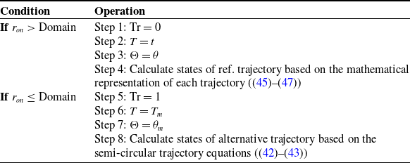
1. Reference Path Planner: This block generates the original reference trajectory that the robot tracks under normal conditions. It includes a trigger parameter, denoted as “Tr,” which is set to zero unless the robot enters the obstacle domain. A unique feature of this block is its ability to save the system’s time (
 $t$
) and heading angle (
$\theta$
) during reference tracking into variables “
$T$
” and “
$\Theta$
,” respectively. When the robot detects an obstacle, the trigger “
$Tr$
” switches to 1, and the last values of
$t$
and
$\theta$
are saved into “
$T_m$
” and “
$\Theta _m$
.” These saved values are critical for generating the next part from the last position of the robot and its orientation.
-
2. Obstacle-Avoidance Mode (OAM) Path Planner: This block is activated when the robot transitions into the obstacle domain (i.e., when
$Tr = 1$
). It uses saved parameters to generate paths that are either semi-circular or semi-elliptical, depending on the value of Z. The path starts from the robot’s last position
$(x_m, y_m)$
and helps navigate around the obstacle. Specifically, if Z equals 1, the path generated is semi-circular. If Z is greater than or less than 1, the path will be a horizontally or vertically oriented semi-elliptical shape, respectively. Upon activation, the simulation time difference between the last (simulation) time and
$T_m$
(last memory of time) resets to zero (
$T = 0$
), allowing the planner to treat the current time as the initial time for the semi-circular trajectory. The
$\theta$
parameter is also leveraged here to ensure proper alignment of the substitute path, facilitating a smooth transition during obstacle avoidance. In (42), the method of drawing the arc is formalized. Moreover, in (43), how to change the direction of the obstacle path using the last position and angle of the robot
$(x_m, y_m, \Theta _m)$
is formulated. -
3. Reference Planner Selector: This block acts as a switch to dynamically select between the original reference path and the obstacle avoidance path. The selection is determined by the trigger signal “
$Tr$
,” as previously defined. The logic for this operation is detailed in Table I, outlining the conditions under which each path is chosen. When the robot enters the defined domain, the first block activates the trigger (
$Tr = 1$
), initiating the obstacle avoidance trajectory. Logical gates, illustrated in the red section of Figure 4, ensure the trigger remains active, preventing the robot from switching back to the reference path until it fully surpasses the obstacle. After completing the obstacle avoidance trajectory, the trigger is deactivated by a pulse generated by the output of a second block. This transition process is governed by the logic shown in the blue section of Figure 4. This framework ensures that the robot can seamlessly shift between paths while maintaining alignment and continuity in navigation, enabling efficient obstacle avoidance and trajectory tracking.(42)
\begin{equation} \begin{aligned} & m = 0 \\ & \text{If } T_0 \geq \frac {3\pi }{2} \Rightarrow m = 1 \\ & \text{If } 0 \leq \cos (T_0) \leq 1: \\ & \quad x_d = -b_{OAM} \cos (T_0) + b_{OAM} \\ & \quad y_d = +b_{OAM} \sin (T_0) + 2(Z+1) b_{OAM} m \\ & \quad \dot {x}_d = +b_{OAM} \sin (T_0) \\ & \quad \dot {y}_d = +b_{OAM} \cos (T_0) \\ & \text{Else:} \\ & \quad x_d = +b_{OAM} \cos (T_0 + \pi ) + b_{OAM} \\ & \quad y_d = +Z b_{OAM} \sin (T_0 + \pi ) + 2b_{OAM}(1 + 2m) + (Z-1)b_{OAM}\\ & \quad \dot {x}_d = -b_{OAM} \sin (T_0 + \pi ) \\ & \quad \dot {y}_d = +Zb_{OAM} \cos (T_0 + \pi )\\ & \text{End} \end{aligned} \end{equation}
(43)
\begin{equation} \begin{aligned} x_r &= x_d \cos \left (\Theta _m - \frac {\pi }{2} \right ) - y_d \sin \left (\Theta _m - \frac {\pi }{2} \right ) + x_m \\ y_r &= x_d \sin \left (\Theta _m - \frac {\pi }{2} \right ) + y_d \cos \left (\Theta _m - \frac {\pi }{2} \right ) + y_m \\ \dot {x}_r &= \dot {x}_d \cos \left (\Theta _m - \frac {\pi }{2} \right ) - \dot {y}_d \sin \left (\Theta _m - \frac {\pi }{2} \right ) \\ \dot {y}_r &= \dot {x}_d \sin \left (\Theta _m - \frac {\pi }{2} \right ) + \dot {y}_d \cos \left (\Theta _m - \frac {\pi }{2} \right ) \end{aligned} \end{equation}


The goal of this method is to demonstrate that the most effective way to navigate around obstacles involves dynamically adjusting the trajectory based on sensor data, similar to how humans drive. Just as drivers visually detect obstacles and immediately define a new path to avoid them before returning to their original route, this method enables the robot to make real-time adjustments.
Algorithm for reference path switching.

Reference planner selector logic circuit: red (top) section shows the trigger activation mechanism, blue (bottom) section illustrates the trigger deactivation process.

The unified control framework utilizing the concepts of obstacle avoidance and reference path switching is brought in Figure 5.
5. Simulation results
To assess the performance of the proposed algorithm, several numerical simulations were conducted across various scenarios. First, the kinematic controller’s effectiveness was evaluated in an obstacle-free environment from different initial positions. These tests demonstrated the controller’s capability to accurately perform the trajectory tracking task. Second, comparative results with the method presented in ref. [Reference Khalaji and Moosavian44] and a nonlinear model predictive controller were analyzed. The findings highlighted that the proposed approach achieved precise trajectory tracking with much lower computational time and complexity.
Next, the performance of the proposed controller, integrated with obstacle avoidance strategies such as the APF method and the proposed PPM, was thoroughly evaluated in large and small-scale static and dynamic environments. This analysis provided detailed insights into the effectiveness of these approaches. Finally, simulations were performed on a smaller-scale map to compare the efficiency and effectiveness of the obstacle avoidance algorithms, identifying the most feasible solution for navigation in constrained environments.
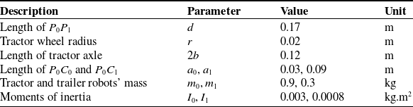
Referring to the kinematic control unit described in Section 3.1 and depicted in Figure 2, the coefficients of the pure integral controllers for each state were first defined, as
 $k_1 = k_2 = 15$
and
 $k_3 = 5$
. Note that these gains are well-tuned, by trial-and-error, such that the most successful response is qualitatively obtained. In addition, the parameters of simulated TTMR are listed in Table II.
Parameters of tractor-trailer mobile robot with their values and descriptions.

Proposed framework for controlling the TTMR in complex environments.

5.1. First case study: evaluation and comparative analysis of the proposed controller
In the first scenario, the performance of the kinematic controller was evaluated under distinct configurations of pose and orientation for the TTMR. The simulations were conducted with various initial conditions, as outlined in Figure 6. In Figure 6(a), the robot was tasked with following a sinusoidal path characterized by frequent and tight curves. The simulation results showed effective trajectory tracking, with the controller successfully managing the sharp turns and frequent curvature changes of the sinusoidal path from various starting points. In a second test case with five different initial conditions depicted in Figure 6(b), the robot navigated a different path shape, resembling patterns commonly seen in agricultural environments such as vineyards and orchards. In this scenario, the controller demonstrated robust performance, managing sharp transitions and maintaining close adherence to the reference trajectory, even in challenging high-curvature sections.
Evaluation of the proposed kinematic controller for tracking: (a) a sinusoidal; (b) Agricultural path.

Performance comparison of the proposed controller (INV) versus NMPC and FLDC for a square-shaped trajectory tracking task: (a) reference and actual path trajectories; (b) longitudinal, lateral, and orientation tracking errors over time.

To compare the performance of the proposed controller with the FLDC presented in ref. [Reference Khalaji and Moosavian44] and a NMPC, simulations were conducted on a square-shaped path, defined by (44) and shown in Figure 7, began with the robot’s initial configuration:
 $\boldsymbol{\eta }(0) = [0.05, 0.2, \pi /2 - 0.5, \pi /2 - 0.2]^T$
. This path is also common in agricultural and warehouse applications.
 \begin{equation} \left \{ \begin{aligned} x_r &= \left (0.5 - \frac {\cos (4t/6)}{28}\right )\cos (t/6) \\ y_r &= \left (0.5 - \frac {\cos (4t/6)}{28}\right )\sin (t/6) \end{aligned} \right. \end{equation}
The proposed controller displayed excellent adaptability in handling sharp turns and maintaining stability during abrupt directional changes. In contrast, the FLDC exhibited slower convergence and greater deviations from the reference path. In addition, the NMPC requires a longer distance and multiple turns to adjust the robot to accurately follow the reference, despite being fine-tuned through numerous trial-and-error processes. As depicted in Figure 7(b), the settling times and error magnitudes for the proposed controller were significantly lower compared to both NMPC and FLDC.
Tracking performance comparison between proposed controller (INV), NMPC, and FLDC.

To quantitatively evaluate the tracking performance of the proposed controller (INV) against the NMPC and the FLDC, multiple time-domain error metrics, including Root Mean Square Error (RMSE), Integral Error (IE), Integral of Absolute Error (IAE), Integral of Time-weighted Absolute Error (ITAE), Integral of Squared Error (ISE), and Integral of Time-weighted Squared Error (ITSE), were computed. The results, summarized in Table III, indicate that both the NMPC and INV controllers deliver robust and precise tracking, with the INV slightly outperforming the NMPC in terms of lower cumulative errors, smoother convergence, and more accurate final positioning (measured by IAE and ITAE). In contrast, the FLDC did not meet the performance standards, showing significantly higher values for IAE, ISE, ITAE, and ITSE in the tested squared path scenario. In addition to tracking performance, computational efficiency is a critical factor for real-time control applications, particularly in embedded or resource-constrained environments. Although the quantitative tracking metrics of the INV and NMPC controllers were nearly identical, the INV controller demonstrated a substantially lower computational burden. Specifically, the average simulation time for NMPC was approximately 18.5 s, whereas the INV controller completed the same task in just 2.5 s. This represents an approximate 86.5% reduction in computational time, achieved under identical conditions using MATLAB 2024b on a 10th Gen Intel(R) Core(TM) i7-10750H processor. Such a drastic improvement underscores the suitability of the INV controller for real-time deployment, especially in scenarios where fast response and low computational overhead are paramount.
Control performance analysis: (a) angular velocities of left and right wheels; (b) required control torques for left and right wheels under NMPC, FLDC, and proposed control (INV) schemes.

All controllers displayed similar velocity profiles during the simulations, except for NMPC, which exhibited abrupt changes in both linear and angular velocities, particularly at the beginning, as shown in Figure 8(a). In contrast to the other two controllers, the proposed controller achieved these velocities with significantly lower control inputs, as indicated by the torque profiles in Figure 8(b). This is especially important in practical applications, where energy consumption has a direct impact on operational costs. The reduced torque provided by the proposed control scheme suggests better use of the natural dynamics of the system, which could lead to decreased mechanical wear and increased system longevity.
5.2. Second case study: obstacle avoidance in complex environments
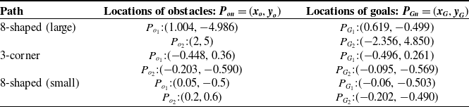
This case study focuses on the proposed controller’s performance in static and dynamic environments in large- and small-scale maps. Some stationary and moving obstacles are introduced in each scenario, with their locations and related parameters detailed in Table IV. The repulsive and gravitational design gains in the APF methods were determined through a trial-and-error process. The values for the repulsive gain,
 $K_{re}$
, range from 0.1 to 1.0, while the gravitational gain,
 $K_G$
, ranges from 5 to 20. Only within these boundaries did the robot maintain collision-free tracking performance. Ultimately, the best results were achieved with
 $K_{re} = 0.5$
and
 $K_G = 10$
. These settings provide a consistent basis for evaluating the obstacle avoidance capabilities of the proposed controller in various trajectory tracking tasks.
Parameters used in obstacle avoidance case study.

5.2.1. Large-scale trajectory
To evaluate the proposed controller’s performance in an environment with static and dynamic obstacles on a large-scale map, the TTMR is tasked with following an eight-shaped trajectory, defined by (45), from the initial position of
 $\eta (0) = [-0.8, -0.8, \pi /2 - 0.2, \pi /2 - 0.2]^T$
. Figure 9 illustrates the reference trajectory alongside the robot’s actual trajectory and the obstacles present. There are three groups of obstacles with varying configurations and dense distributions. The second group consists of moving obstacles, represented by solid purple circles, while the first and third groups contain static obstacles, shown as solid red circles, all with restrictive boundaries of
 $b_r = 0.11$
m. The obstacles in the first group are modeled with a radius of
 $R_{on} = 0.04$
m. The third group includes four obstacles, with some modeled at a radius of
 $R_{on} = 0.01$
m and one more at a larger size of
 $R_{on} = 0.28$
m.
 \begin{equation} \left \{ \begin{aligned} x_r &= 5 \sin (t/15) \\ y_r &= 5 \sin (t/30) \end{aligned} \right. \end{equation}
Large-scaled eight-shaped trajectory tracking with obstacle avoidance: left: reference and actual path trajectories with static and moving obstacles; right: magnified views of critical obstacle avoidance regions.

In this scenario, the robot effectively avoided collisions with stationary obstacles using the proposed APF and PPM methods, despite facing some minor challenges with the APF method. As shown in Figure 9, the dark red ring represents the restricted boundary (
 $b_r$
), within which maneuvering is prohibited, while the orange ring indicates the safe boundary (
 $b_s = 0.0305$
), where the robot operates freely using the APF method. For the first group of obstacles, PPM guided the robot to avoid the first obstacle, then it reverted back to the reference trajectory to avoid a collision with the second obstacle, which was not on the reference path. The robot then planned a new semi-circular path to avoid colliding with the third obstacle. For the third group, PPM devised a new path that allowed the robot to navigate around all the obstacles at once and then return smoothly to the reference path. This flexibility indicates that, depending on the spacing between obstacles or whether the reference path is obstructed by numerous obstacles, the algorithm can either treat them as a single unit to navigate around or as individual obstacles to plan alternative trajectories to avoid collisions with each one.
Although both APF methods demonstrated satisfactory performance in avoiding collisions with stationary obstacles, they were unable to prevent the robot from colliding with moving obstacles. As illustrated in Figure 9, the robot entered a prohibited zone and collided with obstacles. In contrast, the PPM demonstrated superior performance. In the PPM, the moving obstacle’s environment was treated as a zone that the robot should avoid. Consequently, it planned a semi-elliptical path to prevent any collisions. This improvement is attributable to the PPM’s ability to plan a new, smooth reference path around obstacles, whereas the APF approach relies on real-time adjustments of repulsive forces to modify the robot’s trajectory. As a result, the PPM method ensures better continuity and smoothness as the robot navigates, leading to more accurate and stable trajectory tracking.
Performance analysis of obstacle avoidance methods: (a) position and orientation tracking errors; (b) linear and angular velocity profiles during navigation.

The performance analysis in Figure 10 highlights the limitations of the APF method. Adjustments in the APF method are made by adding an
 $\alpha _{OM}$
to the robot’s orientation, while the
 $x$
and
 $y$
coordinates are directly taken from the reference path. As the trajectory generation speed increases, these coordinates change more rapidly, causing sharp variations in angular velocities (Figure 10(b)). In contrast, changes in linear and angular velocities in the PPM method are minimal due to the smooth transition between the reference and alternative paths, which contributes to safer navigation. In addition, the adjustments to
 $\alpha _{OM}$
often conflict with directional changes, as seen at approximately 50, 90, and 150 s in Figure 10(a), where each point corresponds to entering the zone of an obstacle. This results in tracking errors and, in particular, a prolonged time for the second approach of the APF to recover and return to the reference path.
5.2.2. Small-scale trajectory
This subsection evaluates the performance of the obstacle avoidance approaches on two more trajectories.
Although APF methods perform satisfactorily in large-scale trajectories, they face challenges in small-scale environments. This limitation arises because assuming a large safe boundary is impractical for effectively activating gravitational and repulsive fields in confined spaces. As supported by ref. [Reference Liu, Chen, Liu, Zhang, Wu and Liu45], the efficiency of the APF method heavily depends on this boundary size, and our simulation results with
 $b_s = 0.01$
confirm this.
Trajectory tracking for a three-corner path with obstacles.

Detailed views of critical obstacle avoidance regions of the first and second obstacles.

For instance, in the three-corner trajectory (46), the robot begins with
 $\eta (0) = [0.8, 0.3, \pi - 0.8,$
 $ \pi - 0.8]^T$
and encounters high-risk regions under APF tracking (see Figure 11, with detailed views provided in Figure 12). The PPM method shows clearer superiority, avoiding risky domains and ensuring smoother performance.
 \begin{equation} \left \{ \begin{aligned} x_r &= 0.07 \left (5 + \cos (9t/25)\right ) \cos (3t/25 - \pi /6) \\ y_r &= 0.07 \left (5 + \cos (9t/25)\right ) \sin (3t/25 - \pi /6) \end{aligned} \right. \end{equation}
 \begin{equation} \left \{ \begin{aligned} x_r &= 0.5 \sin (t/5) \\ y_r &= 0.5 \sin (t/10) \end{aligned} \right. \end{equation}
Small-scaled eight-shaped trajectory tracking with obstacle avoidance: left: reference and actual path trajectories with static obstacles; right: magnified views of critical obstacle avoidance regions.

Performance analysis of obstacle avoidance methods: (a) position and orientation tracking errors; (b) linear and angular velocity profiles during navigation.

In another scenario with a trajectory defined by (47), the robot starts from
 $\eta (0) = [{-}0.8, -0.8,$
 $\pi /2 - 0.2, \pi /2 - 0.2]^T$
, as depicted in Figure 13.
While the APF method performs slightly better compared to the three-corner path, particularly around the first obstacle, it still enters high-risk zones, increasing the likelihood of collision. In contrast, the PPM avoids these zones by dynamically adjusting the trajectory creation speed, ensuring smoother navigation. The APF approach forces the robot to accelerate abruptly to track the reference path while avoiding obstacles, leading to higher errors and energy consumption compared to the PPM, as seen in Figure 14(a), (b), respectively. This is because APF methods primarily control the direction of motion rather than the velocity, making it challenging to operate in confined spaces or when obstacles are closely spaced. Furthermore, the APF method lacks control over the robot’s distance from obstacles; this distance is instead determined by the cumulative effects of gravitational and repulsive forces. In contrast, the PPM generates alternative trajectories based on the desired distance between the robot and obstacles, ensuring safe navigation in confined spaces or challenging environments such as those with moving obstacles.
6. Conclusion
This study has successfully developed and validated a comprehensive control framework for TTMRs that integrates trajectory tracking with obstacle avoidance. The proposed inverse kinematic control strategy, complemented by pure integral controllers, ensures precise tracking of desired trajectories, even under nonholonomic constraints. The introduction of three obstacle avoidance methods – namely, two customized APF approaches and a novel PPM – provides robust solutions for navigating through static and dynamic environments. The PPM approach, in particular, demonstrates superior performance in dynamically adjusting the reference trajectory to avoid obstacles while maintaining continuity and smoothness in the robot’s motion. This superiority is due to the way PPM defines an alternative path, whereas the APF method relies on cumulative forces to change the robot’s orientation to avoid collisions, resulting in less control over the precise path that the robot follows.
The simulation results highlight the effectiveness of the proposed control framework in achieving accurate trajectory tracking and collision-free navigation. The study also underscores the importance of considering both kinematic and dynamic control strategies in the design of autonomous navigation systems for TTMRs. Future research directions will focus on addressing hardware-specific challenges, such as sensor noise and actuator delays, on a physical TTMR platform in real-world scenarios with various ground conditions. The findings of this study contribute significantly to the field of autonomous robotics, showcasing its potential for real-world applications in logistics, agriculture, and industrial settings.
Author contributions
Aliakbar Ghasemzadeh: Writing – review and editing, Visualization, Methodology. Alireza Azimi: Writing – original draft, Visualization, Methodology. Roya Amjadifard: Writing – review and editing, Methodology, Validation, Supervision. Ali Keymasi-Khalaji: Writing – review and editing, Methodology, Validation, Supervision.
Financial support
This research received no specific grant from any funding agency, commercial, or not-for-profit sectors.
Conflicts of interest
The authors declare no conflicts of interest exist.
Ethical approval
Not applicable.
Appendix
List of symbols and parameters used in the article.