


Introduction
Electoral systems employing districts are known to produce partisan distortions of voters’ voices: a party’s seat-share often does not accurately reflect its vote-share, and thus, supporters of some parties are overrepresented in parliament at the expense of their counterparts supporting other parties (see, for example, Carey and Hix Reference Carey and Hix2011; Gallagher Reference Gallagher1991; Riera Reference Riera2015). Correction mechanisms notwithstanding, this partisan distortion of representation is considered a key characteristic of almost all districted systems.Footnote 1
Alongside the well-established partisan distortion lies an almost entirely overlooked geographic one. This latter dimension is the focus of this study. We illuminate, theorize, and empirically analyze geographic distortion in the conversion of votes to seats: the discrepancy between the origin of a party’s votes (the districts they come from) and the districts in which a party occupies its seats, or put differently, the degree to which parties overrepresent their supporters residing in some parts of the country at the expense of supporters residing in other parts. Unlike partisan distortion, which captures the discrepancy in representation of voters supporting different parties, the geographic dimension of distortion captures discrepancy in representation within parties. Importantly, although related, this concept is theoretically different and empirically distinct from malapportionment: we focus on party-specific rather than national geographic representation, and draw on actual party votes and seats.
A simple example might be in order. In the 2017 Norwegian parliamentary elections, nine parties secured seats in the 169-seat Storting. On one end of the size distribution are the Conservative, Labor, and Progress parties (with forty-nine, forty-five, and twenty-seven seats, respectively). On the opposite end size-wise are the Green and the Left parties, with a single seat per party. Figure 1 takes a close look at two of the four parties in the middle: The Christian Democratic Party (KrF) and the Liberal party (Venstre), securing eight seats each. The figure presents the shares of KrF’s and Venstre’s votes originating in each of Norway’s nineteen districts (in gray) and the respective shares of the parties’ seats obtained in each district (in black).
Votes and seats for the Christian Democratic (KrF) and Liberal (Venstre) parties in Norway’s 2017 election.
Note: Each bar represents the district’s share of votes or seats of the party’s total.
Data source: Constituency-Level Election Archive.

Figure 1. Long description
Panel A: A map of Norway showing the distribution of votes and seats for the Christian Democratic party (KrF) in the 2017 election. The map includes various constituencies labeled with their respective vote percentages and seat allocations. Key constituencies include Akershus, Aust-Agder, Buskerud, Finnmark, Hedmark, Hordaland, Møre og Romsdal, Nordland, Nord-Trøndelag, Oppland, Oslo, Østfold, Rogaland, Sogn og Fjordane, Sør-Trøndelag, Telemark, Troms, Vest-Agder, and Vestfold. The map uses bars to represent the number of seats and percentages to represent votes. Panel B: A map of Norway showing the distribution of votes and seats for the Liberal party (Venstre) in the 2017 election. Similar to Panel A, this map includes various constituencies labeled with their respective vote percentages and seat allocations. The same key constituencies are present, and the map uses bars to represent the number of seats and percentages to represent votes.
The left panel demonstrates a substantial gap for the KrF: the party overrepresents its constituents in five districts (for example, Telemark and Vest-Agder) with a ratio of the party’s seats-to-votes in these districts ranging between 1.7 and 5.7. Correspondingly, KrF supporters residing in the remaining fourteen districts are underrepresented by the party’s seat distribution. The right panel presents analogous quantities for Venstre. Although each of eight districts received 12.5 per cent of the party’s seats, its supporters in Oppland, for example, cast 2 per cent of the party’s votes, and those in Vestfold cast 4 per cent of its votes. Overall, six of the nineteen districts enjoy more Venstre seats compared to votes cast in them at the expense of the remaining thirteen districts.
Two issues specific to this case are worth mentioning (we address them systematically below). First, the source of the discrepancy in the case of these two parties is idiosyncratic to this case. Almost all seats beyond the fraction of votes a district contributed to Venstre or KrF are leveling seats designed to minimize partisan distortion by getting the parties’ share of seats in parliament to reflect more closely their respective share of votes. This highlights the fact that even when partisan distortion is minimized, geographic distortion may still be substantial, and in some cases, the very mechanism that reduces the former increases the latter. Secondly, the discrepancy in the case of these two parties is not due to the malapportionment embedded in the Norwegian electoral systems. In fact, among the six districts amplified within Venstre, four are underrepresented nationally by malapportionment, and there is no systematic correlation between the districts positively malapportioned and those amplified within either party.Footnote 2
In this study, we map geographic misrepresentation and ask: (i) What is the political significance of within-party geographic discrepancy in representation? And, (ii) how can one systematically evaluate geographic discrepancy of representation? Surrogate representation (Mansbridge Reference Mansbridge2003) notwithstanding, a geographic discrepancy between a party’s origin of votes and the districts in which it occupies its seats is politically significant in several aspects. Co-partisans residing in different districts often differ in their local needs served by their respective representatives (Heitshusen et al Reference Heitshusen, Young and Wood2005), such that within-party representational gaps imply disadvantage to underrepresented districts in terms of attendance to their local needs. Furthermore, representatives tend to focus their parliamentary efforts on committees that can serve the interests of the districts in which they are elected (Stratmann and Baur Reference Stratmann and Baur2002). Lastly, the geographic discrepancy in representation of co-partisans is particularly significant if, as we show below, the amplified and the diminished voices differ ideologically.
Utilizing geocoded data (Kollman et al Reference Kollman, Hicken, Caramani, Backer and Lublin2019) and public-opinion data (ESS 2018–2020) from twelve Western democracies that employ electoral districts under either PR or FPTP, we first conduct a simple set of analyses, demonstrating the political significance of geographic distortion of representation. Drawing on 110 parties,Footnote 3 we show discrepancies in the within-party representation of urban v. rural co-partisans, as well as differences in their positions on issues. Overall, there are different voices among supporters of a party residing in different districts, whereby some are heard loudly at the expense of their co-partisans residing elsewhere.
Once we have demonstrated its political significance, we propose a general framework for analyzing geographic representation and develop a measure of geographic disproportionality, GeoDisp. GeoDisp indicates the degree to which the geographic distribution of a party’s seats diverges from that of its votes. Utilizing electoral data from the same set of parties in the twelve democracies, as well as over-time data from three of the cases, we find substantial levels of within-party geographic disproportionality, holding regardless of country-level malapportionment. Furthermore, we find that geographic disproportionality declines with party size, increases with the share of party support originating from small districts, and is generally higher under electoral systems characterized by a large number of small districts. In more tangible terms, we demonstrate, through a thought experiment that keeping party votes and seats constant, an average of eight percent of parliamentary seats would have been assigned to different districts were we to reduce geographic disproportionality to a minimum.Footnote 4
The structure of this paper is harnessed for the theoretical development and empirical analysis of a new concept. The next section lays out the concept of within-party geographic representation and explains why it matters. The following sections present the data we make use of, demonstrate the political significance of geographic representation, derive a general measure (GeoDisp), and develop and test hypotheses regarding GeoDisp. We then analyze geographic disproportionality in terms of actual parliamentary seats. The final section concludes.
Geographic Representational Distortion
The rawest manifestation of public voice is that which is reflected at the voting booth. The discrepancy between party votes cast by voters and seats obtained by parties is perhaps the most straightforward operationalization of misrepresentation. Under this framework, the greater the discrepancies between parties’ vote- and seat-shares, the greater the distortion. We refer to this familiar dimension as partisan disproportionality.
Political scientists have proposed various measures for partisan disproportionality (see Taagepera and Grofman Reference Taagepera and Grofman2003 for an extensive and systematic review). At the national level, countries employing PR with a larger district magnitude are characterized by smaller partisan disproportionality (see, for example, Benoit Reference Benoit2000; Carey and Hix Reference Carey and Hix2011; Powell and Vanberg Reference Powell and Vanberg2000; see also, at the district level, Grofman and Selb Reference Grofman and Selb2010). A more recent set of analyses calls attention to the fact that under PR systems, not only does the average or median district magnitude, but also the variation in it, affect partisan disproportionality (Kedar et al Reference Kedar, Harsgor and Sheinerman2016; Monroe and Rose Reference Monroe and Rose2002).
While partisan representation examines the discrepancy between a party’s vote- and seat-shares, our approach examines the discrepancy between a district’s share of a party’s votes and its share of the party’s seats. We now turn to laying it out.
Geographic (Mis)representation
We propose a transposition of the partisan framework. Our approach identifies each partisan vote by the district it originates from and each seat by the district in which it is occupied. We thus compare the district slices of a party’s pie of votes to the district slices of its pie of seats and examine the discrepancies between them. Parties that occupy their seats in the same districts where their votes originate are geographically representative and have their two pies aligned with each other. The greater the discrepancy between the origin of a party’s votes and the location of its seats, the lesser the party’s geographic representativeness of its supporters. Seen from the voter’s perspective, cases in which a party has limited geographic representation are ones where supporters of the party residing in some districts get more or fewer representatives of their party in their respective districts compared to votes contributed to the party by these districts. Put differently, some of the party’s supporters have their voice amplified, and their co-partisans have it diminished.
Malapportionment
Before we turn to discussing the political significance of this discrepancy, we wish to dwell on the distinction between our analysis of party-level geographic representation and the most prominent concept drawn upon to analyze geographic representation: malapportionment. Malapportionment taps at the ‘discrepancy between the shares of legislative seats and the shares of population held by geographical units’ (Samuels and Snyder Reference Samuels and Snyder2001, 652). As such, it has served as an underpinning concept for the analysis of geographic distortions of formal representation. Indeed, malapportionment has been used as an important compass for comparativists to identify countries whose electoral system – overtly or covertly – deviates from an equal vote–seat ratio across its districts (Lust-Okar Reference Lust-Okar2006; Riera and Lago Reference Riera and Lago2023). Our analysis of geographic representation is distinct from malapportionment in two important aspects. First, it allows us to capture misrepresentation (and later disproportionality) not only of the country as a whole but also by party. As we empirically demonstrate below, different parties are characterized by different levels of misrepresentation of their voters residing in different districts. These differences have a systematic component to them, and are consistent over time. Secondly, our measure taps the discrepancy between actual votes (rather than population) and seats. As such, it is sensitive to specific characteristics of the particular election under study, namely, support rate for different parties and voter turnout.
The anecdotal case of Norway presented above suggests that geographic misrepresentation within parties holds separately of malapportionment of districts. We further address this point systematically in the analysis below. We control for malapportionment in the empirical analysis of our proposed measure of geographic disproportionality and examine the relationship between national-level overrepresentation of a district and its amplification within parties. Both these analyses bolster the finding of geographic disproportionality within parties separate of malapportionment.
Why Study Geographic Representation Within Parties
The study of partisan (mis)representation relies on a key assumption. In the words of Powell (Reference Powell2004), it assumes that ‘the same party means the same thing to voters in different districts within a country’. However, Powell contends:
If the same party label means something different in … two districts, then the results of ‘canceling’ across districts will be misleading at best …. If the party representatives fail to coordinate in their legislative activity, the problem is compounded. (281)
Indeed, surrogate representation (Mansbridge Reference Mansbridge2003) holds that a representative represents voters of her party (for example, on ideological grounds) regardless of the district in which their ballots were cast, delivering representation to voters with whom the representative has no electoral relationship. This powerful notion has also been helpful in explaining a variety of other representational connections in different contexts (Baker Reference Baker2020; Schildkraut Reference Schildkraut2016). For the issue at hand, however, there are reasons to suspect that local representatives are better suited to represent their party supporters compared to their counterparts elected elsewhere. This can be seen in at least three components of representation – service, allocation of resources, and policy/positions (Eulau and Karps Reference Eulau and Karps1977).
Service responsiveness, which includes the non-legislative services that a representative provides for individuals or groups (for example, casework), is almost always directed at individuals or groups within one’s district. Allocation of resources or pork-barrel exchanges, too, are often geographically targeted. It is reasonable to expect that even if supporting the same party, voters in different regions of a country differ in their preferences for the allocation of resources across geographical lines. Voters in the south, for example, might prefer investment in resources that promote the south, while those residing in the north might prefer infrastructure to be delivered to the north. These differences, in turn, project onto representatives’ efforts in parliament (Stratmann and Baur Reference Stratmann and Baur2002).
One might argue that these two aspects of representation can be provided by the local representative(s) regardless of their party. Yet re-election considerations may lead representatives to perform ‘party service in the constituency rather than constituency service’ (Arter and Raunio Reference Arter and Raunio2018, 1). Thus, voters underrepresented by their party might have their service needs fall through the cracks: neither their local representatives from other parties nor their own party representatives from elsewhere fully represent their needs. Additionally, neighbors supporting different parties plausibly prioritize different kinds of investments in their region. Hence again, voters’ representation by their own party is significant for allocation of resources compatible with their interests.
Lastly, co-partisans residing in different districts may share some beliefs across district boundaries, but diverge on others. There is little reason to suspect that supporters of a party, and particularly a party that is a coalition of interests, share the same issue positions on all dimensions, nor that they prioritize the same set of issues to begin with. We hold (and empirically show) that at least in some constellations, differences on such positions among supporters of the same party will align with geographic location.
Political scientists have incorporated districts into the analysis of representation in various ways. First and foremost is the overarching discussion about collective v. dyadic representation. While the former assumes that the legislature as a whole represents the electorate, the latter examines the extent to which the positions of individual legislators are proximate to the preferences of their respective constituents (Achen Reference Achen1978; Hanretty et al Reference Hanretty, Lauderdale and Vivyan2017; Weissberg Reference Weissberg1978), as a form of substantive representation (Pitkin Reference Pitkin1967). More specifically, districts have been shown to be a crucial factor for candidate position-taking (Achen Reference Achen1978), parliamentary speech (Fiva et al Reference Fiva, Nedregård and Øien2025), targeted spending (Catalinac and Motolinia Reference Catalinac and Motolinia2021), and votes in the legislature (Gerber and Lewis Reference Gerber and Lewis2004). In light of the considerations laid out here, we incorporate districts into party-level analysis of vote–seat discrepancy.
Empirical Strategy and Data
Our empirical analysis is two-pronged. In the first part, we analyze the political significance of geographic representation. In the second part, we theoretically develop a measure of geographic disproportionality (GeoDisp) and examine it empirically. Our data include the latest election in each of twelve established democracies that employ a districted electoral systemFootnote 5 and for which we were able to gather full data on districting and election results at the district level, as well as public-opinion data. This amounts to 113 parties that won seats in their national elections (for a list of parties, see Table A1 in the online appendix).Footnote 6 Although all systems are districted, the United Kingdom (and Ireland by some accounts) obviously differ in their electoral system from the rest. In the analysis below, we break down the results by country or eliminate these two cases to allow for the effect of different electoral formulae, yet we find no systematic difference.
To conduct the analysis outlined above, we draw on different sources of data. We list the key sources here in brief, and elaborate below on how we utilize them.
Electoral Data
We utilize district-level election results from the Constituency-Level Elections Archive (CLEA) Lower Chamber Elections Archive (Kollman et al Reference Kollman, Hicken, Caramani, Backer and Lublin2019a). We also utilize CLEA’s GeoReferenced Electoral Districts Dataset (Kollman et al Reference Kollman, Hicken, Caramani, Backer, Lublin, Selway and Vasselai2019b), from which we extract urban/rural categorization.
Public Opinion
To gauge differences in voters’ ideological preferences, we utilize data from the European Social Survey (ESS) waves 9 and 10 (2018 and 2020, respectively). These data include 12,350 respondents in our twelve countries.Footnote 7
How Geographic Representation Matters
Drawing on a broad cross-section of cases, we examine two aspects of the political significance of geographic representation and piece them together. First, we evaluate the degree to which, within parties, urban and rural districts are over/underrepresented. We then add to this analysis the degree to which party supporters residing in urban v. rural districts differ in their issue positions.
Gaps in Representation and Differences in Opinion
While different geographical distinctions may be politically significant in different countries, we focus on the rural–urban cleavage, central in many democracies. Ideally, we would utilize the same identifier for urban v. rural districts in both our vote–seat discrepancy analysis (Figure 2) and in our analysis of public opinion (Figure 3). Neither, however, are available by level of urbanity. We thus follow common practices to bring the two to a commensurable unit of analysis.
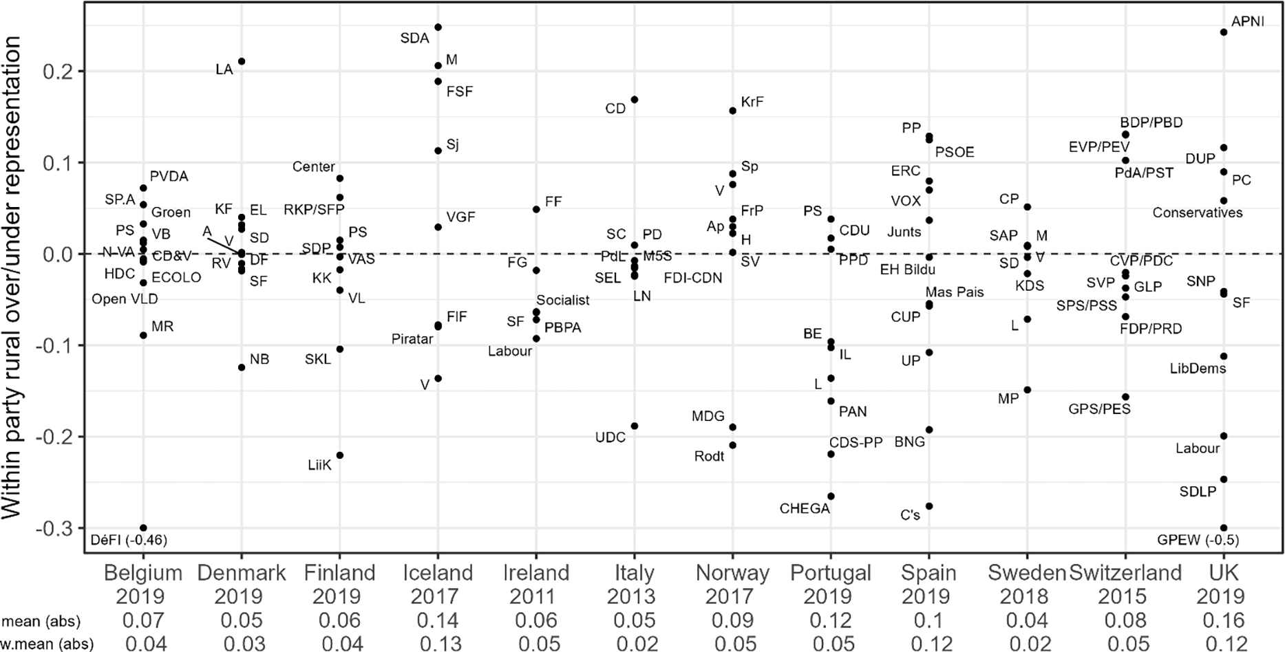
Rural over/underrepresentation within parties in twelve Western democracies.
Note: Parties plotted above the zero line overrepresent their rural voters. For two parties with extreme values (Belgium’s DeFI and the United Kingdom’s GPEW), actual values appear in parentheses. Mean and weighted mean (by party vote-share) of absolute values are noted per country.

Within party: Ideological differences and over/underrepresentation.
Note: The shade of the data points marks the degree of confidence in ideological differences between co-partisans. Of those that reach the highest range of statistical confidence, labels mark parties with a seat-share of 10 per cent or more.

We begin with vote–seat discrepancy. The average population density of a geographical area is a widely used proxy for urbanity, with its accuracy improving as the level of spatial aggregation decreases (see, for example, Huijsmans and Rodden Reference Huijsmans and Rodden2024). Since electoral districts represent the lowest available unit for which seat-share data are available, we calculate district density, drawing on the number of eligible voters per district divided by the size of the district in squared kilometers (obtained from CLEA and CLEA’s GeoReferenced Electoral Districts Dataset, respectively [Kollman et al Reference Kollman, Hicken, Caramani, Backer and Lublin2019a, Reference Kollman, Hicken, Caramani, Backer, Lublin, Selway and Vasselai2019b]). We consider districts below their country’s median density as rural, and those equal to and above the respective median as urban (see, for example, Huijsmans and Rodden Reference Huijsmans and Rodden2024).Footnote 8
Figure 2 presents these gaps for each of the parties (N = 110), grouped by country.Footnote 9 For each party, the figure presents the difference between the share of its seats obtained in sparsely populated districts and the share of its votes cast in them, such that a positive (negative) score implies within-party over(under)representation of rural districts over urban ones. The figure demonstrates several things. First, 33 per cent of the cases (thirty-seven parties) are at least 10 percentage points away from the zero line either upward or downward, implying a substantial within-party geographic mismatch between the origins of a party’s votes and the home of its seats. The range of discrepancies is large and in both directions in most countries (Ireland and Sweden are somewhat closer than others to the zero line).
Secondly, an auxiliary analysis shows that although large parties are characterized by smaller misrepresentation on average compared to smaller ones (Corr (vote-share, absolute gap) = −0.32), this relationship is quite noisy, with some medium and even large parties characterized by high misrepresentation between the two sets of districts. Two such examples are the British Labour Party, which underrepresents its rural voters (−0.2), and the Icelandic Social Democratic Alliance, which overrepresents its rural voters (0.25).
Thirdly, the results reveal heterogeneity within party family across countries (see Figure A2 in the online appendix).Footnote 10 Most party families overrepresent their rural supporters in some countries and underrepresent them in others (for example, Liberal and Social Democratic party families). Two exceptions are the Green and Agrarian/Center parties. The former received little support in small-magnitude districts and is diminished in terms of seats (Kedar et al Reference Kedar, Harsgor and Sheinerman2016). This is, in turn, reflected within the party: its urban supporters receive more seats than their contribution to the party’s votes. The geographic distribution of support for Agrarian/Center parties is mixed, yet they overrepresent their rural supporters. Lastly, a similar heterogeneity is observed when averaging the results (simple average or weighted by party size, see figures at the bottom of Figure 2) by country, with Sweden scoring lowest and Iceland and the United Kingdom the highest.
In sum, a substantial set of parties, small and large, across countries, over/underrepresent their rural or urban voters at the expense of one another. The direction of the representational bias is not constant across parties, nor does it correlate with parties’ political stances. While this result highlights the scope of geographic misrepresentation, in the analysis below, we demonstrate the systematic factors affecting its magnitude.
The vote–seat discrepancy which we find hampers representation more significantly if those residing in the amplified districts differ in their positions from those residing in the diminished ones. To examine this possibility, we utilize public opinion data (ESS 2018, 2020) on four key issue areas in both first- and second-dimension politics covered comparatively in the survey: redistribution, gay rights, immigration, and European integration (see Table A3 in the online appendix for question wording). We transformed all four policy questions to a 0–1 scale, where higher values represent more conservative positions. Utilizing the question item regarding place of residence, we assigned respondents into two groups based on their self-reported residence – country village, farm, or home in the countryside (‘rural’), and a big city, suburbs, or outskirts of a big city (‘urban’). This leaves us with the positions of co-partisans supporting each of ninety-one parties on each of the four issue areas, 364 ideological comparisons altogether.
Figure 3 presents the results of this analysis. The horizontal axis of each panel marks the difference between the mean position of party supporters residing in rural and urban areas, such that where the former hold positions more conservative than the latter, the gap is positive. The vertical axis is identical to that in Figure 2, such that a positive (negative) value marks over(under)representation of rural at the expense of urban co-partisans. Thus, for example, in the top left quadrant are parties whose rural voters are overrepresented compared to their urban counterparts and the positions of their rural supporters are more progressive than those of their urban counterparts. All 364 ideological comparisons in our analysis are marked in the four panels (ninety-one within-party gaps per panel), yet for clarity, we highlight those that are substantively and statistically most significant: cases of a greater certainty of ideological divergence (p < 0.05) are marked in black, and of those, parties whose parliamentary seat-share exceeds 10 per cent are titled (for simplicity, we employ here the generic party family name).
The figure is rich in details and findings, yet it tells a clear story. Overall, in sixty-five (18 per cent) of the comparisons, we find systematic within-party ideological differences that reach standard levels of statistical significance (0.05). Importantly, however, these cases are spread across parties, such that 56 per cent of the parties have at least one policy domain on which their rural and urban supporters differ in their positions. This is yet another manifestation of the complexity of geographic representation. Consider as an example the Partido Socialista (PS) in Portugal, which gained 108 seats (47 per cent) in the lower chamber in the election under study. Its rural supporters are on average 0.15 points more conservative than their underrepresented urban co-partisans on gay rights and seek less redistribution than the latter (gap of 0.06). On European integration and immigration, however, the two groups do not systematically differ. More generally, within-party ideological differences are not specific to a small set of parties or countries, nor do they encompass all issue domains. Co-partisans residing in different regions are in agreement on some issues and differ on others. Particularly noticeable are supporters of Social Democratic parties, who diverge on immigration, and interestingly, supporters of Conservative parties, who diverge on redistribution.
Depending on the issue, the data are clustered to a different degree on either the left or the right side of each panel, indicating the systematic degree to which rural and urban co-partisans consistently differ in their positions. Compared to their urban co-partisans, ruralites support greater levels of redistribution. The latter might be due to scarcity of services or lower average income in rural areas. They also hold that the process of European integration should be slowed down and support more restrictions on immigration. While there are differences on gay rights, the direction of the gap does not strongly correlate with residence. In some cases, it is ruralites who hold conservative positions compared to their urbanite counterparts, while in others it is vice versa.
Lastly, our analysis makes no specific assumptions about issue salience. It is possible that the issues co-partisans differ in their positions on are also the ones most salient to them, yet it is also possible that they are of secondary salience. Although the data we have at hand do not allow us to analyze issue salience systematically, the four issues on which our analysis is conducted often take center stage in electoral campaigns, and so it is not unreasonable to assume that these issues are of major importance to voters. And if parties are decentralized such that different issues are emphasized in different parts of the country, the problem of geographic representation is compounded. In this case, amplified and diminished voices within the party differ not only in their issue positions but also in what issues matter to them.
Overall, the analyses in Figures 2 and 3 reveal within-party differences of opinion combined with gaps of representation. In the concluding section of the study, we reflect on potential implications of this finding.
A General Measure of Geographic Disproportionality
Having examined the political significance of within-party geographic mismatch between votes and seats drawing on specific, albeit well-established, divisions, we turn to measure it in a general fashion. In this section, we introduce our framework, derive our measure, and demonstrate its behavior.
A Framework
What is the extent of the geographic discrepancy between where a party’s votes originate and where its seats are obtained, and how does it differ across parties? In this section, we theoretically and empirically develop a measure of geographic disproportionality (GeoDisp) that allows us to answer these questions in a general framework that goes beyond specific applications. We then evaluate the GeoDisp scores via different comparisons, and explain systematic variation in it. The logic of our measure is straightforward: it compares the shares of a party’s votes originating from different districts to the shares of its seats obtained in them.
A stylized example might be helpful. Imagine party A running in two districts: D1 and D2, with four and twenty seats, respectively. For simplicity, assume that the country is perfectly apportioned with 1,000 votes per parliamentary seat. Assume further full turnout, and that the party received 35 per cent of the votes cast in D1, and 42 per cent of the votes cast in D2, amounting to 1,400 (0.35*4,000) and 8,400 (0.42*20,000) votes, respectively, 9,800 in total. Now, assume that given vote-shares of other parties in each of these districts and the electoral formula, these votes translate to two seats in D1 and six seats in D2, eight seats altogether. District D1 therefore contributed 0.14 (1400/9800) of the party’s votes and obtained 0.25 (2/8) of the party’s seats. Similarly, D2 contributed 0.86 (8,400/9,800) of the party’s votes and obtained 0.75 (6/8) of its seats. Supporters residing in D1 are therefore overrepresented at the expense of their co-partisans residing in D2. In the formalization below, we present a general measure, following which we apply it to evaluate the gap presented in this example.
Figure 4 presents the logic behind our proposed measure. Imagine a country divided into N districts (i = 1…N) in which K parties (j = 1…K) compete for seats in an S-seat parliament. Let v ij denote the votes cast in district i for party j, and s ij denote the seats obtained in district i by party j. Thus, voters in district 1 cast a total of v 1. votes (v 11, v 12, …, v 1K ), and the district gets a total of s 1. seats (s 11, s 12, …, s 1K ), both for Parties 1 through K. Similarly, Party 1 gets a total of v .1 votes (v 11, v 21, …, v N1) and obtains s .1 seats (s 11, s 21, …, s N1), both from districts 1 through N. Panel a presents this stylized setup.
Partisan and geographic disproportionality.

Figure 4. Long description
Panel A: Votes and seats setup. A table with 3 rows and 5 columns. Column headers are p 1, p 2, p K, and Total. Row labels are d 1, d N, and Total. The table contains values for votes (V) and seats (S) for each party (p) and district (d). Row 1: d 1, V 11, S 11, V 12, S 12, V 1 K, S 1 K, V 1 period, S 1 period. Row 2: d N, V N 1, S N 1, V N 2, S N 2, V N K, S N K, V N period, S N period. Row 3: Total, V 1 period, S 1 period, V 2 period, S 2 period, V K period, S K period, V period, S period. Panel B: Partisan disproportionality. A table with 3 rows and 5 columns. Column headers are p 1, p 2, p K, and Total. Row labels are d 1, d N, and Total. The table contains values for votes (V) and seats (S) for each party (p) and district (d), with partisan disproportionality indicated for each district. Row 1: d 1, V 11, S 11, V 12, S 12, V 1 K, S 1 K, partisan disproportionality in d 1. Row 2: d N, V N 1, S N 1, V N 2, S N 2, V N K, S N K, partisan disproportionality in d N. Row 3: Total, V 1 period, S 1 period, V 2 period, S 2 period, V K period, S K period, partisan disproportionality. Panel C: Geographic disproportionality. A table with 3 rows and 5 columns. Column headers are p 1, p 2, p K, and Total. Row labels are d 1, d N, and Total. The table contains values for votes (V) and seats (S) for each party (p) and district (d), with geographic disproportionality indicated for each party and overall. Row 1: d 1, V 11, S 11, V 12, S 12, V 1 K, S 1 K, V 1 period, S 1 period. Row 2: d N, V N 1, S N 1, V N 2, S N 2, V N K, S N K, V N period, S N period. Row 3: Total, V 1 period, S 1 period, V 2 period, S 2 period, V K period, S K period, V period, S period, geographic disproportionality.
Standard partisan disproportionality measures identify votes by the party they are cast for and seats by the party obtaining them. They then calculate the discrepancy between the two for each party and, depending on the measure, apply some arithmetic formula to these gaps. This is highlighted in panel b. Greater gaps between party vote- and seat-shares (typically calculated at the national level, but can also be calculated at the district level) lead to greater disproportionality scores.
We transpose this analysis. We identify votes and seats by their district. Under this framework, each party has a vector of votes it receives from various districts and a vector of seats it occupies in various districts. This is presented in panel c. At the party level, we compare the share of votes the party received in each district out of the overall votes it received with the analogous seat quantity.
Measuring Geographic Disproportionality
Political scientists have devoted extended efforts to analyzing partisan representation in general and disproportionality between votes and seats in partisan representation in particular (see, for example, Gallagher Reference Gallagher1991; Grofman Reference Grofman1983; Rose Reference Rose, Lijphart and Grofman1984; Taagepera and Grofman Reference Taagepera and Grofman2003). Different measures capture different aspects of the discrepancy between the share of votes received by each party and the share of seats it obtains, and they vary in their mathematical properties, level of granularity, and implied normative assumptions.
Taagepera and Shugart (Reference Taagepera and Shugart1989, 105) propose a measure D which aggregates across parties their absolute differences between their vote- and seat-shares. In terms of the quantities in Figure 4, the index at the national level is calculated as:
 $D={1 \over 2}\sum\nolimits_{j}\left| { v_{.j} \over V}-{s_{.j} \over S}\right|$
This index can be thought of at the district level as well:
 $D_{i}={1 \over 2}\sum\nolimits_{j}\left| {v_{ij} \over v_{i.}}-{s_{ij} \over s_{i.}}\right|$
We transpose their measure to get at the disproportionality between the votes and seats contributed by different districts. Most importantly for our purposes, and drawing on an inner column of the table, we define geographic disproportionality of party j as:
 $GeoDis{p_j} = {1 \over 2}\sum\nolimits_i {\left| {{{{v_{ij}}} \over {{v_{.j}}}} - {{{s_{ij}}} \over {{s_{.j}}}}} \right|}$
And at the national level, based on the final column of the table, we calculate the vote- and seat-shares as part of the overall votes and seats cast in and assigned to a district:
 $GeoDisp = {1 \over 2}\sum\nolimits_i {\left| {{{{v_{i.}}} \over V} - {{{s_{i.}}} \over S}} \right|}$
This latter measure indicates the degree to which there is a discrepancy in the country as a whole between where votes come from and where seats go.Footnote 11
Applying Equation (3) to our illustration of party A above, we get:
 $\textit{GeoDisp}_{A}={1 \over 2}\left(\left|0.14-0.25\right|+\left|0.86-0.75\right|\right) =0.11$
, indicating a mismatch of 11 per cent. Put differently, 11 per cent of the votes of party A were not assigned to the districts in which they originated. Our analyses below shed light on qualities of the measure.
Geographic Disproportionality: Theoretical Exploration
Our measure ranges between zero and one, and the score of the measure is the percentage of votes shifted from one district to another (Taagepera and Shugart Reference Taagepera and Shugart1989, 105). But what is a high per cent and what is a low one? We shed light on the magnitude of geographic representativeness in different contexts by comparing its scores theoretically across constellations and empirically to related measures. We begin with the former.
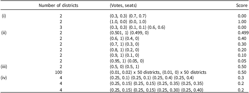
Table 1 presents stylized scenarios and their corresponding GeoDisp scores of a single party. Each section of the table compares two or more scenarios, each consisting of the shares of votes each district contributes to a party’s total votes and the share of seats it receives of the party’s total obtained seats. The right column of the table presents the GeoDisp score of the respective scenario. Section i presents three scenarios (two and three districts) and conveys the boundaries of our measure. In the first scenario, the share of the party’s seats is identical to the share of the party’s votes in each district, and unsurprisingly, a perfect geographic proportionality is attained (a GeoDisp score of 0). Conversely, in the second scenario, all votes contributed to a party originate from one district and all seats are assigned to another. This is obviously not consistent with electoral law and results in absolute disproportionality (GeoDisp = 1). The third scenario is similar to the first, only with more districts, and it demonstrates the invariability of our measure to the number of districts, a point we return to in Section iii.
Configurations of geographic disproportionality

Table 1. Long description
This publication-style table presents electoral district scenarios divided into four categories labeled (i) through (iv). Across three main columns—Number of districts, (Votes, seats), and Score—it compares how vote-seat distribution pairs relate to a final calculated score. Scenarios test varying district counts (2, 3, 4, or 100). Scores range from 0.00 (perfect proportional match) up to 1.00. As district vote shares fluctuate against winning seat shares, scores scale accordingly.
Section ii presents six scenarios of two districts each. In the first scenario, one district contributes 0.501 of the party’s votes and receives all its seats, while the other contributes 0.499 of its votes and receives none of the party’s seats. This scenario results in a GeoDisp score of 0.499. As we move from the first to the last scenario, the discrepancies decline, and the GeoDisp score declines accordingly, reaching a score of 0.05 in the last one. Plainly put, the smaller the discrepancy, the smaller the score.
Section iii provides two examples whereby the vote–seat discrepancies amount to a score of 0.5. In the first, the country is divided into only two districts, each contributing to the party 0.5 of its votes and receiving either zero or all of them. In the second, the country is divided to 100 districts, each contributing 0.01 of its votes and receiving either 0.02 or none of the party’s seats. This example, in which in both scenarios half of the voters do not get a seat in return for their vote and half get twice as many albeit under dramatically different district constellations, demonstrates the general property whereby our measure is invariant to the number of districts. This property enables us to draw on our measure to compare disproportionality across countries with drastically different numbers of districts.
Lastly, Section iv presents three scenarios with a varying degree of misrepresentation. The discrepancy in all districts declines from a total of 0.6 in the first scenario to a total of 0.4 in the second, and GeoDisp declines respectively from 0.3 to 0.2. The third scenario builds on the second, increasing and decreasing the discrepancy by the same amount in two of the districts, thus maintaining the total discrepancy at 0.4. As can be seen in the table, GeoDisp does not change, demonstrating that it captures the total geographic discrepancy a party embodies regardless of the relative degrees of the district-level discrepancies it consists of.
Disproportionality Across Parties and Countries
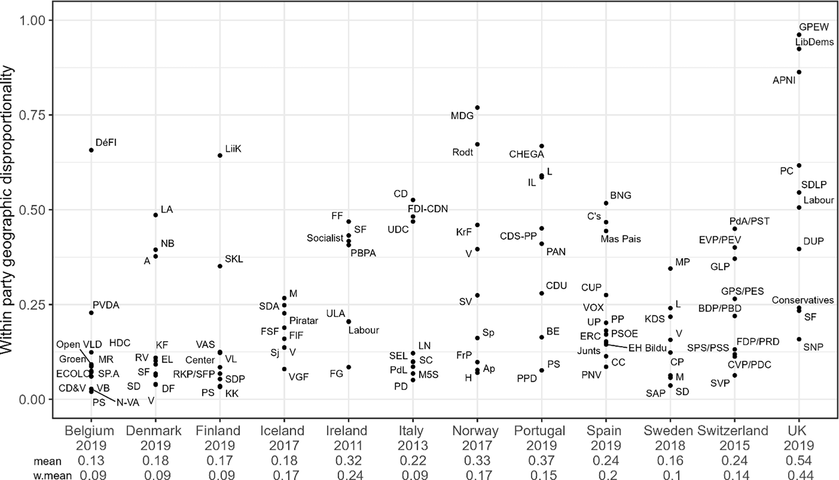
Given our theoretical focus, our analysis below is at the party level. We utilize raw data of district-level votes and seats (Kollman et al Reference Kollman, Hicken, Caramani, Backer and Lublin2019a) drawn upon in Figure 2. Figure 5 presents 113 party-level GeoDisp indices in our twelve countries. The overall average party-level GeoDisp score is 0.25 (SD = 0.21), with 36 per cent of the parties scoring higher than average. While we calculate geographic disproportionality as a party-level measure, we also consider countries as characterized by different levels of and degree of variation in geographic misrepresentation. First, countries vary in their average party score, with Belgium and the United Kingdom at the low and high end of the distribution, respectively (figures and vote-share weighted figures are noted under Figure 5). Secondly, they differ in how much variation there is within them, with countries such as Iceland and Sweden exhibiting little difference in their parties’ disproportionality scores, and others such as Norway and Portugal exhibiting a wide range.
Geographic disproportionality across twelve Western democracies.
Note: Geographic disproportionality within parties by country. Mean and weighted mean (by party vote-share) are noted per country. Geographic disproportionality is calculated based on Equation (3).

Figure 5. Long description
Panel A: A scatter plot representing the relationship between within-party geographic disproportionality and various political parties across twelve Western democracies. The horizontal axis represents different countries and years, while the vertical axis represents the within-party geographic disproportionality. The data points are labeled with the abbreviations of the political parties. The plot shows a range of disproportionality values, with some parties exhibiting higher disproportionality than others. There are visible clusters and outliers, indicating variations in geographic disproportionality among the parties.
Although small parties are less representative than their larger counterparts (more on this below), geographic disproportionality is not a property reserved for small parties only. Moderate-size parliamentary parties with a relatively high disproportionality score include, among others, the Icelandic Center Party and SD Alliance (with 11 per cent of the seats in parliament and scores of 0.27 and 0.25, respectively), and Fianna Fail and Labour in Ireland (with scores of 0.47 and 0.2 respectively). In the United Kingdom, the large Labour and Conservative parties also have high disproportionality scores (31 and 56 per cent of the seats in parliament and scores of 0.51 and 0.24, respectively). Lastly, the results vary substantially both across and within party families (see Figure A4 in the appendix). While some party families are characterized by low levels of geographic disproportionality (for example, the radical right), others exhibit significant discrepancy between where their votes originate and where their seats are assigned (for example, the left). Additionally, party families differ in the variation of their geographic disproportionality (for example, the Conservatives v. the Liberals).
The analysis of GeoDisp scores at the party level reported here is consistent with the results of misrepresentation by rural–urban groupings presented above. They correlate at 0.73, with the absolute value of the rural–urban gaps presented in Figure 2 (the correlation is positive in all twelve countries, with a median score of 0.76). This obviously does not imply that our rural–urban intraparty cleavage illustration is the only manifestation of geographic disproportionality, yet it is reassuring that GeoDisp tightly captures representational gaps in this prominent cleavage.
Putting Geographic Disproportionality in Context
To shed light on the relative quality of party-level geographic representation, we conduct two comparisons of GeoDisp scores and revisit the Norwegian case presented at the outset.
Geographic disproportionality at the party and national levels
A comparison of our party-level GeoDisp index (avg. GeoDis p = 0.25) to the national-level one (the empirical versions of Equations (3) and (4), respectively) corroborates our premise of party-level misalignment of votes and seats. Unsurprisingly, compared to the party-level indices, national-level scores are negligible, hovering around an average of 0.06 (s.d. = 0.03), showing near perfect geographic congruence between votes and seats (see Table A5 in the appendix for all twelve scores). The stark gap between the scores at the two levels is an indication that substantial geographic distortion within parties is masked by the pooling of votes and of seats across parties at the national level.
Partisan v. geographic disproportionality
Drawing on the same data, we switch to comparing the two dimensions: our party-level geographic disproportionality score and partisan disproportionality at the national level (Taagepera and Shugart Reference Taagepera and Shugart1989, 105). We calculate the partisan disproportionality at the national level, as is commonly done (see, for example, Taagepera and Shugart Reference Taagepera and Shugart1989, Table 10.1, 106–7; Gallego et al Reference Gallego, Rico and Anduiza2012). This is akin to comparing the empirical versions of Figures 4(c) (party level) and 4b (national level), respectively, in our cross-section of cases.
The average national-level partisan disproportionality score is 0.08, ranging from 0.005 and 0.008 (Sweden and Denmark, respectively) on the low end to 0.23 (Italy), with the United Kingdom second (0.15), on the upper end. Seven of our countries score 0.07 or lower. Lastly, both countries characterized by a high partisan disproportionality and ones characterized by a low one have parties with a range of geographic disproportionality scores, and, as seen in the Norwegian case at the outset, in some cases the two dimensions are even in tension with one another.
Norway 2017 revisited
Finally, we return to the Norwegian case highlighted at the outset and examine the party scores of GeoDisp in it. The Liberal Party (Venstre) and the Christian Democratic Party (KrF), whose geographic (mis)representation is presented in Figure 1, score 0.4 and 0.46, respectively, with a nine-party average GeoDisp score of 0.33 (weighted average = 0.17). The three largest parties – the Conservative, Labor, and Progress – show relatively high levels of geographic congruence between where their votes originate and where their seats are assigned (with GeoDisp scores of 0.07, 0.08, and 0.1, respectively). On the opposite end of the distribution, the Greens and the Left (Rødt), with a single seat each, are particularly unrepresentative geographically (0.77 and 0.67, respectively). This is hardly surprising, given that a single-seat party is almost inevitably geographically incongruent with the party’s origins of votes.
The two comparisons above, along with the Norwegian results, underscore the value added of analyzing geographic representation at the party level. Partisan representation highlights discrepancies in representation of supporters of different parties, overlooking ideological and interest-based differences between co-partisans residing in different districts. Geographic representation at the national level (through either GeoDisp or malapportionment) highlights discrepancies in representation between voters residing in different districts, overlooking differences between neighbors supporting different parties. Our analysis of party-level geographic representation complements the two. It focuses on representational discrepancy between voters residing in different districts while also considering within-party differences.
Systematic Variation in Disproportionality
What accounts for the variation in geographic disproportionality across parties? The discrepancy between the origin of a party’s votes and the location of its seats depends on both idiosyncratic factors (for example, turnout and vote-shares of different parties in the district) and systematic ones. In what follows, we address the latter.
GeoDisp consists of district-level gaps between votes the party wins and seats it obtains and is therefore affected by discontinuity in the conversion of votes to seats. While such discontinuity takes place for both small and large parties, any given set of votes (and seats) that are not accurately translated into seats constitute a larger fraction of the total votes (and seats) of small parties than of large ones. Our first expectation is therefore that GeoDisp declines with party size. Secondly, given that votes are more accurately converted to seats in large-magnitude districts, we expect that GeoDisp will increase with the share of a party’s votes originating from small districts. Lastly, this logic is traceable to the electoral system. We expect that countries where a large fraction of the parliament is elected via small-magnitude districts will be characterized by parties with greater geographic disproportionality compared to countries with fewer seats elected in small districts.Footnote 12 We therefore examine three hypotheses.
HYPOTHESIS 1. Small parties will be characterized by greater geographic disproportionality compared to large ones.
HYPOTHESIS 2. Parties whose votes originate from small-magnitude districts will be characterized by greater geographic disproportionality compared with parties whose votes originate from large ones.
HYPOTHESIS 3. The larger the fraction of parliamentary seats elected via small-magnitude districts, the greater geographic disproportionality will be.
To analyze the systematic component of GeoDisp, we regress party-level GeoDisp scores against the party’s vote-share (H1), the fraction of the party’s votes originating from small-magnitude districts (equal to or smaller than three up to seven seats, H2), and the share of parliamentary seats originating from small-magnitude districts (three up to seven, H3). Importantly, our different specifications control for key suspects. Given the analysis of the Norwegian Venstre and the KrF above, we include in the analysis the fraction of the party’s obtained seats that are leveling seats as well as the country-level comparable quantity: the fraction of parliamentary seats that are leveling seats. We also include malapportionment. In all specifications, standard errors are clustered by country.
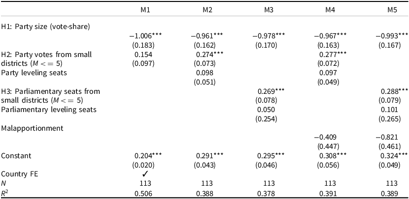
Table 2 presents the results of this analysis. As can be seen in the table, consistent with H1, geographic disproportionality is negatively correlated with party vote-share. The effect is remarkably stable across specifications and is substantial in its magnitude: an increase of one percentage point in vote-share is associated with a decline of one percentage point in GeoDisp. With respect to district magnitude, in the interest of space, the table presents a cut-off of districts with a magnitude smaller than 5 (more on the other cut-offs below). An increase in the share of a party’s votes originating from small districts results in greater geographic disproportionality (H2). Thirdly, the country-level reflection of the latter (H3) holds as well: countries in which a greater share of parliamentary seats are elected in small districts are characterized by parties with greater geographic disproportionality. The latter two results hold controlling for party and parliamentary leveling seats, respectively. Lastly, note that while Models 3 and 5 include country-level indicators as controls (parliamentary leveling seats and parliamentary share of seats in small districts), in Model 1 we replace those with country fixed effect. Our results for H1 hold, and our results for H2 hold in their direction, though statistical significance is lower. The coefficients on our control variables tell a similar story across models: malapportionment, leveling seats in the parliament as a whole, and leveling seats which the party won are not systematically correlated with geographic disproportionality.
Geographic disproportionality, party size, and small-M districts

Table 2. Long description
This regression table reports results across five statistical models (M1–M5) with N = 113. It tests hypotheses (H1–H3) on party size, small-district votes/seats ($M \le 5$), leveling seats, and malapportionment. Across all models, party size (vote-share) shows a consistent, highly significant negative effect (around -0.96 to -1.01). Small-district votes (H2) and seats (H3) have significant positive impacts (0.26–0.29). M1 includes country fixed effects and achieves the highest R2 at 0.506.
Note: Dependent variable: geographic disproportionality. Standard errors clustered by country in parentheses. *p < .05, **p < .01, ***p < .001.
Robustness
We conducted a set of analyses similar to those reported in Table 2, albeit with different cases and different cut-offs.
Countries included
We reran the analysis eliminating the United Kingdom and keeping only PR cases. We also ran it eliminating both the United Kingdom and Ireland. The results (reported in the online appendix Table A6) hold when the United Kingdom is omitted, and, with the exception of H3 which keeps its direction but loses its statistical significance, when both cases are omitted.
Cut-offs
We reconducted the analysis with all other cut-offs of district magnitude between 3 and 7 (see Tables A7 in the online appendix). The results reported in Table 2 are stable: in almost all specifications, GeoDisp is negatively associated with parties’ vote-shares, and positively associated with their shares of seats originating in small districts and with the share of parliamentary seats in small districts.
Additional Analyses
In this section, we bolster our findings by turning to two additional analyses. First, we further investigate the relationship between GeoDisp and malapportionment. We then move to analyze GeoDisp over time in a subset of our cases.
Malapportionment
One might wonder whether malapportionment is at the heart of within-party amplification of districts. After all, if a district is nationally overrepresented by the electoral system, it might be, by extension, amplified within parties. In addition to the multivariate analysis above, we calculate for each of the 906 districts in our data the degree of their parliamentary over/underrepresentation. Specifically, we calculate the district’s share of seats in parliament minus the district’s share of eligible voters in the country, such that a positive (negative) difference implies that the district is over(under)represented in parliament:
 ${\matrix{Dist.\; \textit{overrepresentation} \cr w/i\; \textit{country}}}={\textit{district}\; \textit{seats}\; (M) \over \textit{seats},\; \textit{total}\; (S)}-{\textit{eligible} \;\textit{voters} \;in\; \textit{district} \over \textit{eligible} \;\textit{voters},\; \textit{total}}$
Applying a similar logic, we then calculate for each district the degree to which it is amplified within each of the parties competing in it (the difference between the district’s share of the party’s seats and its share of the party’s votes), such that a positive (negative) difference implies that the district is geographically amplified (diminished) within the party:
 ${\matrix{Dist.\; \textit{amplification} \cr w/i\; \textit{party}}}={\textit{party}\; \textit{seats}\; in\; \textit{district} \over \textit{party}\; \textit{seats},\; \textit{total}}-{\textit{party}\; \textit{votes}\; in\; \textit{district} \over \textit{party}\; \textit{votes},\; \textit{total}}$
Thus, each district has a single national representation score indicating its over/underrepresentation in parliament and a set of party-level amplification scores.
First, we examine if nationally overrepresented districts tend to be amplified within parties. 51 per cent of the districts (465/906) are nationally overrepresented per Equation (5). Among those, none are amplified within all parties that compete in them. Rather, they each exhibit a mix, amplified within some parties and diminished within others.Footnote 13 Of the 441 underrepresented districts, twenty-three are diminished within all parties in their country, and the rest are diminished within some and amplified within others.
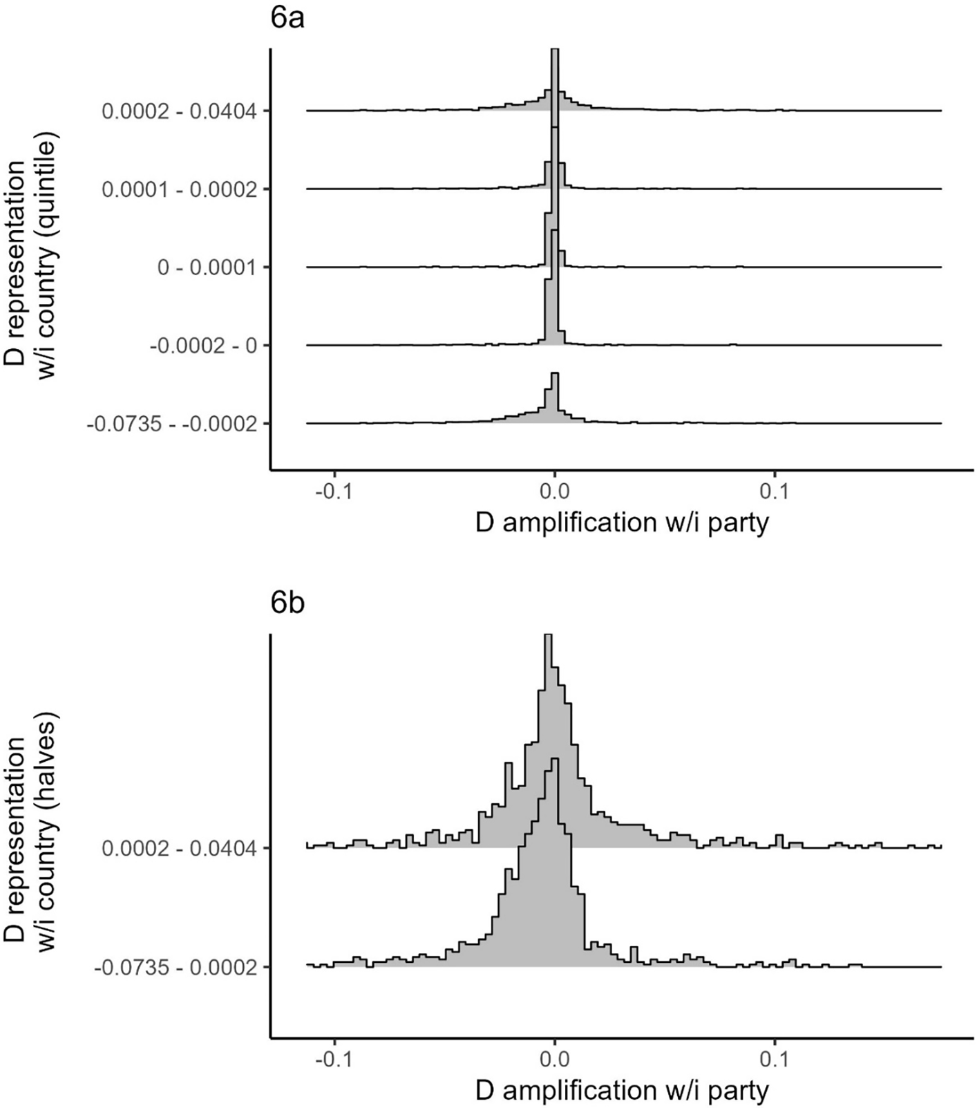
Next, we divide districts into quintiles according to their national representation score per Equation (5). For each fifth of our 906 districts, we examine the distribution of within-party amplification scores per Equation (6).Footnote 14 If the two are strongly related, we should find a systematic difference among the five groups of districts: the nationally most overrepresented quintile should be on average the most amplified within parties, and the nationally least represented quintile should be on average diminished within parties. Figure 6 presents these five distributions in descending order of national over/under representation. As is shown in the figure, the distributions of party-level amplifications hover around zero regardless of the district quintile at the national level and overlap almost in their entirety. They do not exhibit a systematic difference that correlates with national representation by the electoral system. For robustness, we drop the United Kingdom, our only majoritarian case, and repeat this exercise (panel b), only this time dividing the remaining 256 districts into two groups by the median of their national representation score. The results hold: we see no systematic pattern whereby nationally overrepresented districts are amplified within parties.
District representation within country and party.
Note: The figure sorts districts by their national-level over/underrepresentation and presents the amplifications within parties for each district. Panel a groups the districts to quintiles and panel b excludes the United Kingdom and splits the remaining districts by the median. For presentation, both panels exclude the 1 per cent most amplified and 1 per cent most diminished districts within parties.

Overall, both these analyses suggest that within-party amplification or diminishing of a district hold empirically both in cases where the district is overrepresented by the electoral system and in ones where it is underrepresented.
GeoDisp over Time
So far, we analyzed GeoDisp cross-sectionally, drawing on a wide range of parties and one time-slice per party. One might wonder, however, if geographic disproportionality is a stable characteristic over time. To this end, we analyze three consecutive elections in Norway (2009, 2013, 2017) and in Sweden (2010, 2014, 2018), and four in Portugal (2009, 2011, 2015, and 2019). These three cases experienced no changes in district boundaries since 2000 and have a medium number of districts compared to others in our data.
The analysis (reported in Figure A8 in the appendix) shows that in all three cases parties’ GeoDisp scores exhibit little change over time, except when the parties’ electoral fortunes change dramatically (for example, the Norwegian Venstre between 2009 and 2013, and the SV between 2013 and 2017). When this is the case, consistent with the analysis in Table 2, the score decreases with an over-time increase in party size. Furthermore, as expected, such electoral changes result in greater changes in GeoDisp scores for smaller parties than for larger ones.
How Many Seats? A Thought Experiment
The analysis above demonstrates a substantial degree of geographic disproportionality. In this last step of our analysis, we seek to transform it to a more tangible quantity of interest and examine its implications in terms of misassigned parliamentary seats.
To address this question, we conduct a simple thought experiment drawing on the intuition of GeoDisp: for each party, we calculate the difference between its share of votes originating from and share of seats obtained in each district. We then calculate for each party the variance in this difference and iteratively reassign its seats from amplified to diminished districts, reducing the variance in this gap and thus the inequality in geographic representation till no further reassignment can reduce it any more. Importantly, we impose two constraints on this exercise: seats are assigned in full integers, as is the assignment of real representatives, and partisan disproportionality is unchanged (that is, the number of seats each party obtained is given).
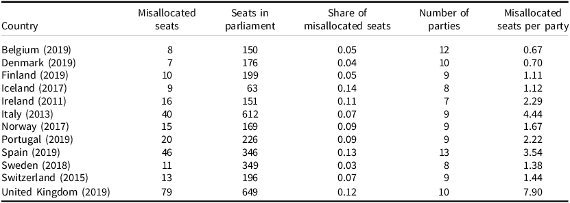
Table 3 presents the results of this analysis for each of our countries. The first column presents the number of parliamentary seats that would have been assigned to supporters of the same parties residing in a different district were parties to more accurately geographically represent their supporters residing in different districts. The third column presents this figure as a fraction of all parliamentary seats. Our exercise suggests that on average 8.3 per cent or 23 of the seats in parliament (7.9 per cent or 18 without the United Kingdom, respectively) should have been reassigned to supporters of the same parties residing in o ther districts, ranging between 3 per cent in Sweden to 14 per cent in Iceland. Seventy-nine parties (70 per cent) have at least one seat that should have been reassigned according to our exercise.
A thought experiment: geographically misallocated seats

Table 3. Long description
This table details electoral seat misallocations across 12 European countries between 2011 and 2019. It tracks total seats in parliament, misallocated seats, their share, total parties, and misallocated seats per party. The United Kingdom (2019) has the highest misallocated seats (79) and per-party average (7.90), while Spain (2019) follows with 46 misallocated seats (13% share across 13 parties). Iceland (2017) records the highest share of misallocated seats at 14% (9 of 63 seats). Conversely, Sweden (2018) and Denmark (2019) show the lowest shares of misallocated seats at 3% and 4%, respectively.
Note: Parties’ total seats are unchanged, only reassigned to districts in accordance with the party’s share of votes cast in the different districts.
Overall, this analysis demonstrates that in all countries included in our analysis, geographic disproportionality in the assignment of parliamentary seats is not merely about the discontinuity stemming from their assignment in integers. Rather, a sizeable number of party seats are misaligned with their vote origin.
Conclusion and Implications
In this paper, we offer a new prism through which the ubiquitous translation of votes to seats can be evaluated: the disproportionate representation of voters supporting the same party and residing in different districts. That some voices among party supporters are amplified and others diminished raises questions about the implications of discrepancies in geographic representation for both voter behavior and policy outcomes. With regard to voters, one might wonder if lacking representation for their region might serve as a disincentive for voters to support a particular party. Geographic (mis)representation might also affect congruence between parliament and public opinion as well as government responsiveness. If, for example, dyadic representation affects the latter, it is likely that greater geographic disproportionality will lead to less responsiveness.
Geographic representation can be analyzed along various dimensions unexplored in this study. Co-partisans residing in geographically peripheral regions of a country might have different priorities regarding investment in geographically based infrastructure (railways, roads, and even airports). Residential interests might also result in differences in positions on environmental preservation v. economic development, and occupations related to residence might affect one’s positions on tariffs and trade. Any such ideological or interest-based dimension on which co-partisans might differ and within-party geographic representation is distorted may have implications for this newly identified dimension of representation.
Geographic representation is likely linked to party-system nationalization. In non-nationalized party-systems, parties run and compete only in some regions, avoiding waste of votes that would not have been converted to seats in other regions for lack of massive support there. We would therefore expect geographic disproportionality to be smaller where politics and the party system accordingly are regionalized. At the same time, other things equal, regional parties are smaller than national ones, and hence they are expected to suffer from greater geographical disproportionality. Overall, then, the actual empirical link between geographic disproportionality and party-system nationalization is unclear, and further investigation is needed.
Last but not least, the analysis in this paper carries normative implications. When evaluating electoral systems, political scientists have taken a clear stand on the value of partisan representation (see, for example, Carey and Hix Reference Carey and Hix2011): high partisan disproportionality, an indication that votes for some parties translate to more seats than others, is a challenge for equal political representation. Our study highlights that the underlying assumption of that analysis, that parties represent all their supporters and do so equally, masks both ideological and representational discrepancies within parties. Thus, geographic disproportionality in itself is an important challenge to equal representation. When considering the values that different electoral mechanisms promote and those they compromise on, geographic representation ought to be on the table of institutional designers.
Supplementary material
The supplementary material for this article can be found at https://doi.org/10.1017/S0007123426101616.
Data availability statement
Replication data for this paper can be found at https://doi.org/10.7910/DVN/Z59UUU
Acknowledgments
For helpful comments and suggestions, the authors thank Jon Slapin, Damien Bol, Pedro Riera, Jim Snyder, Gustavo Novoa, Clareta Treger, Thomas Gschwend, André Walter, and participants at the University of Zurich workshop on political representation, EPIC 2025, MZES seminar, ETH/UZH colloquium, and the annual meetings of the MPSA, EPSA, and ECPR.
Financial support
This work was supported by the Israel Science Foundation (grant number 3437/25).
Competing interests
None to disclose.





 Open access

