





Introduction
Cohort life tables, which follow the survival of a cohort from birth to death, provide the most reliable means of estimating stage-specific mortalities (Begon et al. Reference Begon, Mortimer and Thompson1996). In field studies of mobile insects, following a cohort of the same individuals throughout their lives is difficult. However, equivalent information can be obtained for a defined unit of population of univoltine insects by repeated estimation of population size from egg-hatch until death, thereby producing a horizontal stage-specific life table, also known as a budget (Richards Reference Richards1961). Accumulations of budgets over many years permit identification of key mortality factors responsible for population change, detection of density dependence (Varley and Gradwell Reference Varley and Gradwell1960; Varley et al. Reference Varley, Gradwell and Hassell1973), and examination of how environmental factors affect mortality (e.g., Harcourt Reference Harcourt1971). Stiling (Reference Stiling1988) summarised information from 63 published life tables involving 58 insect species, of which 25 were Lepidoptera, 18 were Homoptera, and only six were Coleoptera, none of which were carabid beetles.
Development of life tables for Carabidae is problematic because quantitative sampling of all life stages is difficult. In many carabid species, the adults are surface-active, but the larval stages are not (Lövei and Sunderland Reference Lövei and Sunderland1996; Luff Reference Luff, Lövei and Toft2005), and estimating numbers of eggs and pupae is extremely difficult (Heessen and Brunsting Reference Heessen and Brunsting1981). Carabid adults are usually sampled by pitfall trapping (Lövei and Sunderland Reference Lövei and Sunderland1996); however, catches depend not only on numbers of insects but also on their surface activity (Mitchell Reference Mitchell1963; Greenslade Reference Greenslade1964), which is affected by environmental factors (Briggs Reference Briggs1961; Nève Reference Nève, Desender, Dufrêne, Loreau, Luff and Maelfait1994; Saska et al. Reference Saska, van der Werf, Hemerik, Luff, Hatten and Honek2013) and beetles’ physiological state (Gilbert Reference Gilbert1956; Murdoch Reference Murdoch1966). Annual indices of adult carabid population size may be derived from “year-catches” in pitfall traps (Baars Reference Baars1979). Alternatively, mark–recapture techniques, often in conjunction with beetle-proof enclosures (e.g., Grüm Reference Grüm1975; Nelemans et al. Reference Nelemans, den Boer and Spee1989; Baumgartner et al. Reference Baumgartner, Bechtel, Van Den Boom, Hockman, Horstmann and Kliewe1997), may be used to estimate populations of carabid adults from pitfall trap catches. Long-term studies of population dynamics of carabid beetle populations have relied on these annual indices or estimates of adult numbers (e.g., Baumgartner et al. Reference Baumgartner, Bechtel, Van Den Boom, Hockman, Horstmann and Kliewe1997; Hockmann et al. Reference Hockmann, Horstmann, van den Boom, Landwehr, Bechtel, Kliewe, Baumgärtner, Brandmayr and Manly1998), which in some cases have been augmented by laboratory or field enclosure–based studies of mortality of immature stages (e.g., Nelemans et al. Reference Nelemans, den Boer and Spee1989; van Dijk and den Boer Reference van Dijk and den Boer1992). Such studies do not provide the insights into stage-specific mortalities that can be derived from budgets.
Carabids of many species inhabit lacustrine (lakeside) beaches (Larochelle and Larivière Reference Larochelle and Larivière2003), yet little is known about their population dynamics. Beaches and similar coastal habitats are often unsuitable for pitfall traps because of wave action, variations in water level, and the absence of a stable surface into which traps can be sunk. But the simplicity of these habitats makes it possible to sample multiple life stages of some carabids by searching the refuges they use during periods of inactivity (Gilbert Reference Gilbert1956; King and Stabins Reference King and Stabins1971; Holliday Reference Holliday2025a) The objective of the current study was to investigate population processes of a common carabid beetle inhabiting stony lacustrine beaches, using quantitative quadrat sampling of three life stages to produce stage-specific life tables for analysis. It presents results of a 16-year study of Chlaenius cordicollis Kirby (Coleoptera: Carabidae) focusing on analysis of mortality factors, including tests for density dependence, key factor analysis, and investigation of the influence of environmental variables.
Methods
Study organism
Chlaenius cordicollis is univoltine, and its natural history in Manitoba, Canada, is described in detail in Holliday (Reference Holliday2025a). Both larvae (Holliday et al. Reference Holliday, Mattingly and Holliday2015) and adults (Eisner et al. Reference Eisner, Hurst and Meinwald1963; Holliday et al. Reference Holliday, Mattingly, Toro, Donald and Holliday2016) produce defensive chemicals, which deter a range of natural enemies. Adult beetles are nocturnal and spend the day under limestone slabs; larvae are less exclusively nocturnal but also frequently hide under stones during daylight hours. Both larvae and adults are primarily scavengers that feed on insect remains that are washed ashore by the lake (Larochelle and Larivière Reference Larochelle and Larivière2003; Holliday Reference Holliday2025a).
In Manitoba, “spring adults” emerge from overwintering sites in May and move down the stony beaches that the beetles inhabit in the summer months. Cues for oogenesis are photoperiodic, and the majority of females in samples in June and July are gravid. In the laboratory, there is a single episode in which females lay all their eggs within a few days, and no more eggs are developed thereafter. There is a peak of larval numbers in samples in mid-summer; almost all of these are “late larvae” in the third instar because first- and second-instar larvae move within the substrate and are small and infrequently seen. Eggs, the lethargic prepupal stage of the third instar, and pupae have not been detected in the field (Holliday Reference Holliday2025a). Overwintered adults do not survive after reproduction (Holliday et al. Reference Holliday, Mattingly, Toro, Donald and Holliday2016). New-generation “fall adults” appear during and following the larval peak and, from late August onwards, move up the beach into overwintering sites, where they are not detectable by quadrat sampling. Winter is spent buried in beach-top gravel ridges in aggregations that can contain more than 100 individuals (Holliday Reference Holliday2025a).
Study site and field sampling
The study site was a beach on the east coast of Hecla Island, Manitoba, which is on the western side of the south basin of Lake Winnipeg. The study site was representative of a 7-km stretch of stony beaches that are described in more detail in Holliday (Reference Holliday2025a). The beach at the study site consisted of limestone slabs (mainly 10–100 cm in diameter) overlaying a mixture of sand and gravel and interspersed with glacial erratic boulders. At the top of the beach was an eroding cliff, above which was a forest stand of spruce, Picea (Pinaceae) and aspen, Populus tremuloides Michaux (Salicaceae).
The study was conducted over 16 years, from May 1984 until September 1999. Sampling took place at approximately weekly intervals during the period when C. cordicollis larvae or adults were active on the beach, with sampling beginning in May and usually extending into September. The sample universe for the study was a 100-m strip of beach centred at 51.0708° N, 96.6854° W and oriented approximately north–south. Although the north–south dimension of the sample universe was fixed, the width from the base of the cliff to the water’s edge varied from 1 m to 18 m, depending on the water level of the lake.
A stratified random sampling system was used, based on coordinates established along the length of the sample universe, with the coordinate origin at the midpoint. On each sample occasion, random numbers between 0 and 50 were taken, and transect samples were located at the selected number of metres north and the south of the origin. Transects extended from the cliff base at the top of the beach to the water’s edge. An average of six transects were taken on each sample occasion. Samples within each transect were taken using a 1-m × 1-m wire quadrat. The quadrat was initially placed at the top of the beach, and after each sample was completed, the quadrat was moved down the beach to sample the adjacent 1-m2 area; the process continued to the water’s edge. Quadrat coordinates included the transect coordinate and the number of metres from the top of the beach. At each quadrat location, C. cordicollis adults and larvae were collected into 120-mL plastic screw-capped containers containing moist gravel. All moveable stones were turned over, and beetles were collected by hand or herded into collection containers. Except where the substrate was sand or immovable boulders, the substrate was thoroughly wetted with lake water to aid in bringing insects to the surface. Collection efforts continued at each quadrat location until no more beetles were detected. For each quadrat, records were kept of its coordinates and the number of adults and larvae collected; the maximum quadrat coordinate for the transect yielded a measure of the beach width at the time and location of sampling. Collection containers were labelled with the quadrat coordinates, and at the end of the sampling session, beetles were released at the site of their collection.
Estimates of population densities
Beetles do not leave the sample universe in summer, so numbers per quadrat in the present study were higher when high lake levels reduced available habitat. To remove this source of variation, numbers of adults and larvae in each quadrat were summed to yield the density measure: numbers per transect. To separate effects of population processes from those of short-term changes in sampling efficiency related to variable weather and water levels, densities were averaged over 15-day intervals from 1 May each year. To depict seasonal patterns, the numbers of adults and larvae in each transect were log-transformed (log10[X + 1]), and the average and standard error of the transformed values for each 15-day interval were plotted against date.
Life tables were constructed using untransformed data. The peak of numbers of late-instar larvae was used to separate overwintered prereproductive and reproductive spring adults from new-generation fall adults. The density of spring adults was the maximum average density of adults per transect in a 15-day interval that occurred before the peak of late-instar larvae. The density of fall adults was the maximum average density of adults in a 15-day interval that occurred after the peak of late-instar larvae. Determinants of the date of the larval peak were investigated by multiple regression.
Numbers passing through the late larval stage were estimated using Southwood’s graphical method (Southwood and Jepson Reference Southwood and Jepson1962). The density of larvae was calculated for each 15-day interval, these numbers were plotted against time, and the area under the curve was calculated. Because almost all larvae detected in quadrats were third instars before the prepupal lethargic stage, the area under the curve was divided by (15.7−4.1)/15, where 15.7 days is the average total duration of the third instar at 21 °C, the average temperature experienced by larvae in the field in July (Holliday Reference Holliday2025a), and 4.1 days is the average duration of the lethargic stage (unpublished data); division by 15 converts the result to time units of 15 days.
The density of eggs that initiated each cohort in the life table was estimated using the method of Varley et al. (Reference Varley, Gradwell and Hassell1973), in which the density of reproducing females is multiplied by the egg content of dissected reproductive females. The sex ratio does not differ from 1:1 (Holliday Reference Holliday2025b), so the density of spring adults was divided by 2 and then multiplied by 49.3, which was the average number of eggs per gravid female in dissections (Holliday Reference Holliday2025a).
These estimates were used to construct life tables for 15 cohorts of C. cordicollis, beginning with annual egg estimates for 1984–1998 and with estimates of late-instar larvae, fall adults, and spring adults for each cohort. Cohorts are referred to by the year of the egg estimate; therefore, estimates for spring adults, although occurring in the following year, are referred to by the number of the previous year. The net reproductive rate, R 0, between densities in adjacent cohorts was calculated for late larvae, fall adults, and spring adults.
Estimates of mortality
Age-specific mortalities for the intervals between the four stages were expressed as k-values (Varley et al. Reference Varley, Gradwell and Hassell1973), obtained by subtracting the log-transformed number per transect at the end of each interval from the log-transformed number at the beginning of that interval. In this way, for each cohort, there were three mortality estimates that sum to the total mortality, K, for the cohort, where E represents the number of eggs, LL represents the number of late-instar larvae, FA represents the number of fall adult beetles, and SA represents the number of spring adult beetles:
 $$K=k({\rm E}-{\rm LL})+k({\rm LL}-{\rm FA})+k({\rm FA}-{\rm SA})$$
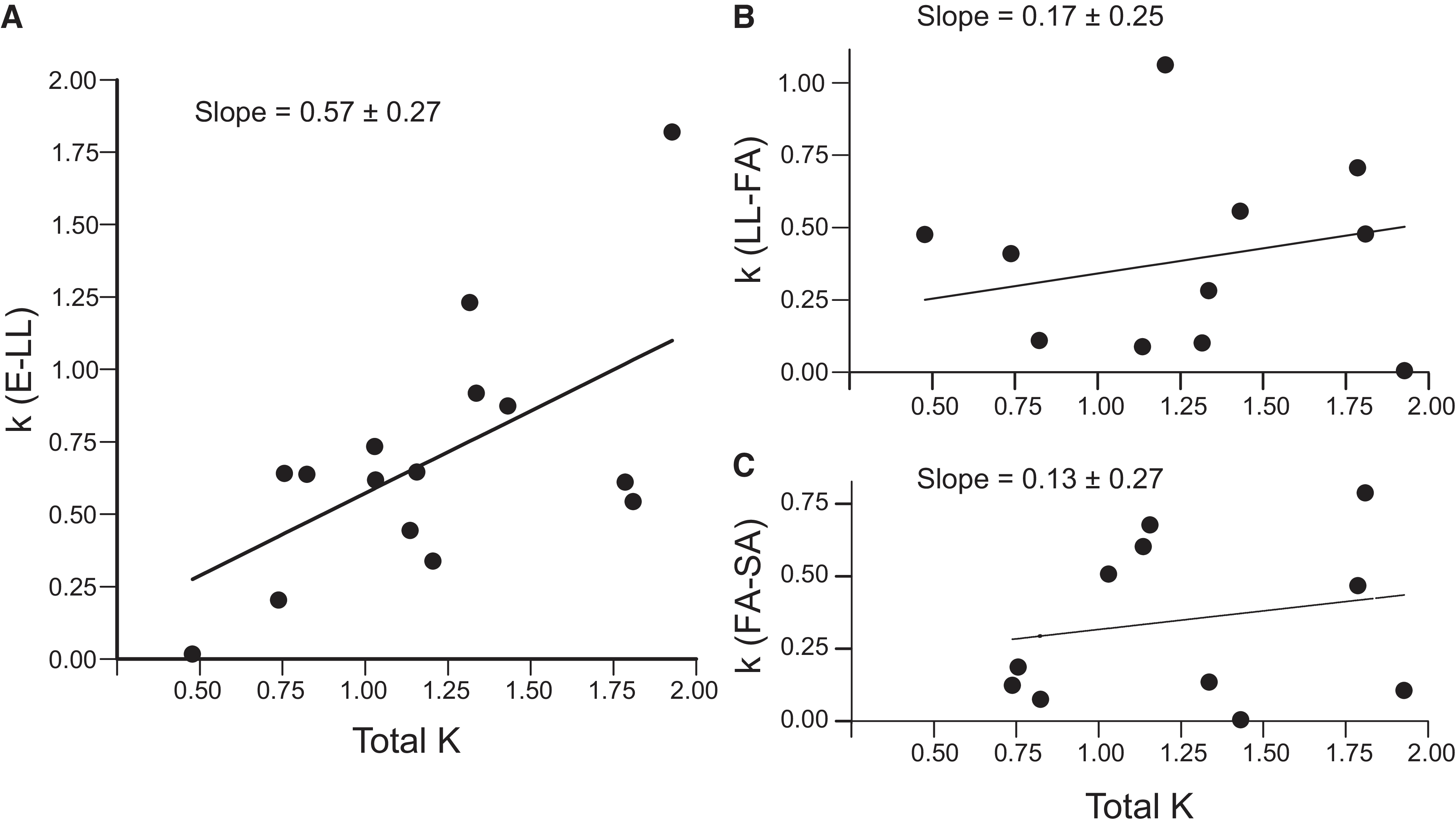
The mortality that was the key factor most influencing population change was identified by regressing each k-value against the total K for the cohort (Podoler and Rogers Reference Podoler and Rogers1975); the key factor has the greatest significant regression slope.
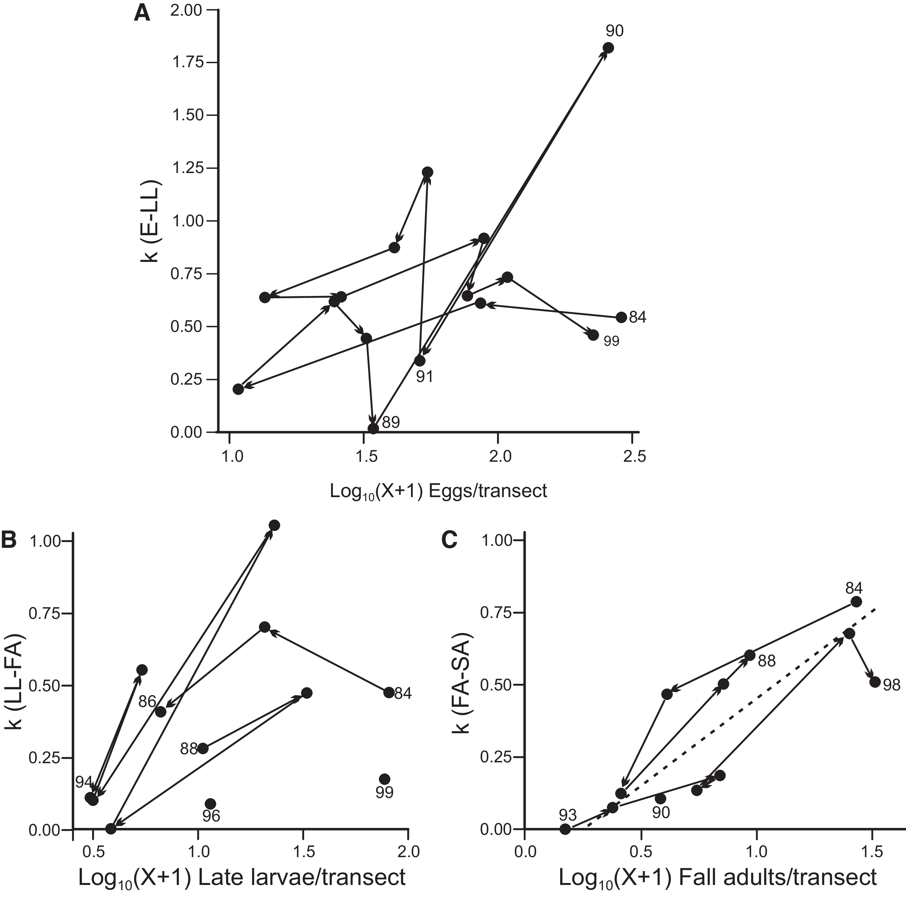
The density dependence of each k-value was investigated by regression of the k-value on the log density at the beginning of the interval in which the mortality occurred and by joining the points in a time sequence (Varley et al. Reference Varley, Gradwell and Hassell1973). Because Nelemans (Reference Nelemans1987) had demonstrated that limited resources for larvae increased mortality and reduced fecundity of later stages of Nebria brevicollis (Fabricius) (Coleoptera: Carabidae), delayed density-dependent effects were investigated in the present study by regressing k-values for later intervals on log densities of all earlier life stages. To assess whether density of a stage in a cohort influenced its subsequent fecundity, k(E − LL) for the following cohort was included in this investigation of delayed density dependence because a density-dependent deviation from the estimated average fecundity would influence this k-value.
Mortality and environmental variables
Multiple regression was used to investigate the relationship of k-values to variables of four types: dates of events in the life cycle of C. cordicollis; times of freeze-up and break-up of ice cover in the south basin of Lake Winnipeg; average beach width and its variability at the study site; and temperature, precipitation, and snow depth. Dates of events in the life cycle of C. cordicollis were expressed as the midpoint day-of-year of the 15-day interval in which they occurred. Dates of freeze-up of the south basin of Lake Winnipeg for each year in 1984–1990 were obtained from the Environment Canada weather observer in Gimli, Manitoba, as reported in McCullough (Reference McCullough2005). The same publication provided dates of ice break-up from 1987 to 1999, derived from satellite imagery. For years where observational data were unavailable, freeze-up and break-up dates for the south basin were estimated from McCullough’s (Reference McCullough2005) predictive regression equations, based on 40-day running averages of air temperatures at Berens River, Manitoba (Environment Canada 2025a).
As described in the “Study site and field sampling” section, beach width on each sample date was measured as the length of each transect. For the multiple regressions, a daily estimate of beach width for all days was required and was obtained from a regression of average transect lengths for each sample date against the average lake level for the same day, as measured at Gimli, Manitoba (Environment Canada 2024). The Gimli hydrological station reports lake levels as metres above sea level (m.a.s.l.). The station is located 58 km south of the study site; both are on the west side of the south basin of Lake Winnipeg and so are likely to respond similarly to seiches (wind-driven short-term oscillations in water level) that are common on the lake (Einarson and Lowe Reference Einarson and Lowe1968). The regression used to predict daily average beach width at the study site (Holliday Reference Holliday2025a), was as follows:
 $${Beach\;width\;(m) = 1465 - 6.697daily\;mean\;water\;level \;at \;Gimli \;(m.a.s.l.)}$$
Temperature, precipitation, and snow depth data were obtained from Environment Canada climate stations. The nearest station that collected temperature and precipitation data throughout the 16-year study was at Arborg, Manitoba, 42 km southwest of the study site and 16 km from the west shore of the south basin of Lake Winnipeg. The Arborg station (Environment Canada 2025b) provided temperature data for multiple regressions for all k-values and precipitation data for k(E − LL) and k(LL − FA). Beach-top overwintering sites of C. cordicollis adults have greater snow accumulations than elsewhere on beaches, and windblown snow from the ice-covered lake enhances accumulation (Holliday Reference Holliday2025a). Hence, the candidate environmental variables for inclusion in the multiple-regression model for k(FA − SA) were subdivided into three periods: before lake freeze-up, during the period of lake ice cover, and after ice break-up. The depth of snow was not measured at Arborg, so records of rainfall, snowfall, and snow depth from the Hodgson2 climate station (Environment Canada 2025c) were used in regressions for k(FA − SA). The Hodgson2 climate station was located 65 km west of the study site and 40 km from the nearest portion of Lake Winnipeg.
Statistical analyses
Statistical analyses were performed with Genstat (VSN International 2024a). Regressions of individual k-values against total K and those of k-values against the densities on which they act are type 2 regressions in which both variates are subject to error. For these, the three-group method of Bartlett (Reference Bartlett1949) was used, and the significance of slopes was determined by estimation of 95% confidence limits using bootstrapping with 200 resamplings (VSN International 2024a).
The focus of the multiple-regression investigations was to identify the environmental factors that were most closely associated with variation in k-values for each stage. A forward selection procedure was first adopted, in which terms were added if the resulting change in residual mean squares exceeded the residual mean squares of the model with the term added (VSN International 2024b). Frequently, this approach resulted in the regression model containing many correlated variables that added little to the overall fit. Consequently, to arrive at a final model, a backwards selection process was used to remove correlated variables that contributed little while retaining those that added most to the coefficient of multiple determination, r 2.
Results
Estimates of population densities
The numbers of late-instar larvae per transect typically followed a more-or-less triangular trajectory with a peak near the middle of the period of larval detection (Fig. 1). The peak usually occurred in July but ranged in date from late June to early August. The date of ice break-up and mean daily temperatures in May and June were candidate independent variables in the multiple-regression investigation of determinants of the date of the larval peak. Of these, the only significant influence was the mean daily temperature in June (F = 11.95; df = 1, 12; P = 0.005). For each 1 °C rise in June temperature, the late-instar larval peak was 4.1 ± 1.2 days earlier. In many years, the late-instar larval peak coincided with a local minimum in the density of adults. Adults counted before this minimum were presumed to be spring adults that had survived winter. The rise in adult densities during or following the larval period was considered to represent recruitment of new-generation fall adults.
Numbers per transect of adult and larval Chlaenius cordicollis from 1984 to 1999. Numbers per transect were log10(X + 1)-transformed, and the average and standard error were calculated for all transects in each 15-day interval during the period of activity. SEM, standard error of the mean.

Figure 1. Long description
The image contains multiple line graphs showing the numbers per transect of adult and larval Chlaenius cordicollis from 1984 to 1999. Each graph represents a different year, with the x-axis labeled as months from May to September and the y-axis labeled as Mean (+ SEM) Log10(X+1) Numbers per transect. The solid line represents adults, and the dashed line represents late larvae. Each graph shows the average and standard error calculated for all transects in each 15-day interval during the period of activity. The trends and patterns vary by year, with some years showing peaks in adult numbers during specific months and other years showing different patterns for larvae.
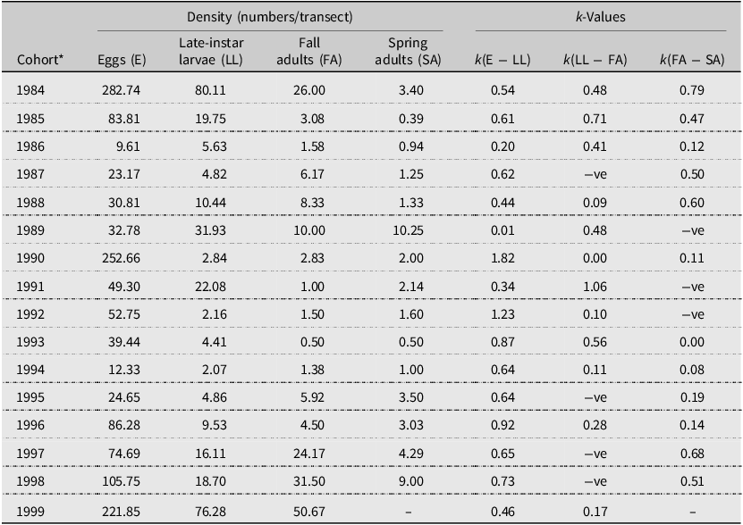
Densities of C. cordicollis varied considerably among years, with relatively large numbers in the first and last part of the study and small numbers in 1986 and 1992–1994 (Fig. 1). For late-instar larvae, the highest density (Table 1) was 39 times the lowest density; for fall adults, the corresponding relationship was 101 times, and for spring adults, it was 26 times. Over all cohorts, the net reproductive rate, R 0, on the basis of late-instar larval numbers was 1.89 ± 0.52 (mean ± standard error) with a maximum of 7.77 for the 1990 cohort; for fall adults, R 0 was 1.71 ± 0.42 (maximum 5.4; 1996 cohort), and for spring adults, R 0 was 1.77 ± 0.51 (maximum 7.71; 1988 cohort). Although all mean values appear to show population growth over the study, none differed significantly from R 0 = 1, the value that signifies constant population size (t-tests: P > 0.1).
Stage-specific life table for Chlaenius cordicollis on a beach on Hecla, Manitoba, Canada, showing densities and mortalities expressed as k-values. Density of eggs, fall adults, and spring adults are estimated maximum densities per transect; density of late-instar larvae is the estimated number passing through the third instar, expressed on a per-transect basis. Negative k-values (“–ve” in the table) would indicate the impossible situation in which densities increased in a stage at the time when reproduction is not occurring. See text for details.

Table 1. Long description
A table comparing densities and mortalities of Chlaenius cordicollis across different life stages and years. The table has 16 rows and 9 columns. The columns are labeled as follows: Cohort, Eggs (E), Late-instar larvae (LL), Fall adults (FA), Spring adults (SA), k (E - LL), k (LL - FA), k (FA - SA). The rows are labeled with years from 1984 to 1999. Each row provides the density values for eggs, late-instar larvae, fall adults, and spring adults, along with the corresponding k-values for each transition between life stages. Notable trends include variations in densities and k-values across different years, with some years showing higher densities and others showing lower densities. Negative k-values are indicated as ‘– ve’ in the table.
Note: Cohorts are designated by the year in which the eggs are laid. Spring adults occur in the year following the year designating the cohort and were not sampled in 2000.
Estimates of mortality
Three stage-specific mortality k-values were estimated for each cohort (Table 1). Mortality between the estimate of eggs and late-instar larvae, k(E − LL), represents the mortality of eggs and first- and second-instar larvae and may also be influenced by deviations in fecundity from the average number of eggs in dissected females, which was used to estimate egg numbers. Mortality from late-instar larvae to fall adults, k(LL − FA), represents mortality of the lethargic stage of third-instar larvae and of pupae and recently eclosed new-generation adults. Mortality from the peak of fall adults to that of spring adults, k(FA − SA), includes mortality in overwintering sites and during movement to and from those sites, as well as mortality in the sample universe during late fall and early spring. Some k-values that involved estimates of fall adults were negative, signifying an apparent increase in density at a time when reproduction was not occurring. These values were excluded from subsequent analyses.
The key factor responsible for most change in population size was k(E − LL) (Fig. 2A). The slope was greater than those for the other stage-specific k-values (Fig. 2B, 2C) and was the only slope that differed significantly from 0 (95% confidence limits; hereafter CL 95%: +0.127, +1.135). In the investigations of density dependence of the three stage-specific mortalities (Fig. 3), the slope of the regression for k(E − LL) did not differ significantly from 0 (CL 95%: −0.07, +1.03), and so there is no evidence of density dependence. The time sequence plot (Fig. 3A) exhibits a somewhat cyclic pattern interrupted by much higher mortality in 1990. The cyclic pattern could indicate a delayed response to egg density in the previous year. However, the nonsignificance of the slopes of regressions of k(E − LL) on log densities of eggs one year (CL 95%: −0.70, +0.36) and two years (CL 95%: −0.33, +0.80) previously did not support this hypothesis. Time sequence plots for k(LL − FA) (Fig. 3B) and k(FA–SA) (Fig. 3C) were discontinuous because of the omission of those estimates of k-values that were negative. Neither of these plots exhibited the cyclic or spiral pattern characteristic of a delayed response. The slope of the regression for k(LL − FA) on log late larval density was not significant (CL 95%: −0.07, +0.89). The slope for the regression of k(FA − SA) on the log of fall adult density differed significantly from 0 (CL 95%: +0.36, +0.81) and is plotted in Fig. 3C. The regression slope, 0.604 ± 0.118, indicates direct density dependence.
Identification of the key mortality factor, using the method of Podoler and Rogers (Reference Podoler and Rogers1975). Stage-specific k-values are plotted against total cohort mortality K: A, mortality from eggs to late larvae, k(E − LL); B, mortality from late larvae to fall adults, k(LL − FA); C, mortality from fall adults to spring adults, k(FA − LL). Each point represents a cohort; in B and C, cohorts with negative k-values are excluded.

Investigation of density dependence of mortality factors by plotting time sequences of k-values against the log-transformed density on which they operated: A, mortality between eggs and late-instar larvae, k(E − LL); B, mortality between late-instar larvae and fall adults, k(LL − FA); C, mortality between fall adults and spring adults, k(FA − LL); the dashed line represents a significant regression relationship. Numbers adjacent to points are the final two digits of the year in which the cohort began. In B and C, the time sequence is discontinuous because negative values of k are excluded.

Figure 3. Long description
Panel A: A line graph shows the mortality between eggs and late-instar larvae, k(E-LL), plotted against the log-transformed density of eggs per transect. The y-axis represents k(E-LL) values ranging from 0.00 to 2.00, and the x-axis represents the log-transformed density of eggs per transect. The graph includes multiple lines, each representing a different year, with the final two digits of the year labeled next to the points. Panel B: A line graph shows the mortality between late-instar larvae and fall adults, k(LL-FA), plotted against the log-transformed density of late larvae per transect. The y-axis represents k(LL-FA) values ranging from 0.00 to 1.00, and the x-axis represents the log-transformed density of late larvae per transect. The graph includes multiple lines, each representing a different year, with the final two digits of the year labeled next to the points. Panel C: A line graph shows the mortality between fall adults and spring adults, k(FA-SA), plotted against the log-transformed density of fall adults per transect. The y-axis represents k(FA-SA) values ranging from 0.00 to 1.00, and the x-axis represents the log-transformed density of fall adults per transect. The graph includes multiple lines, each representing a different year, with the final two digits of the year labeled next to the points. A dashed line represents a significant regression relationship.
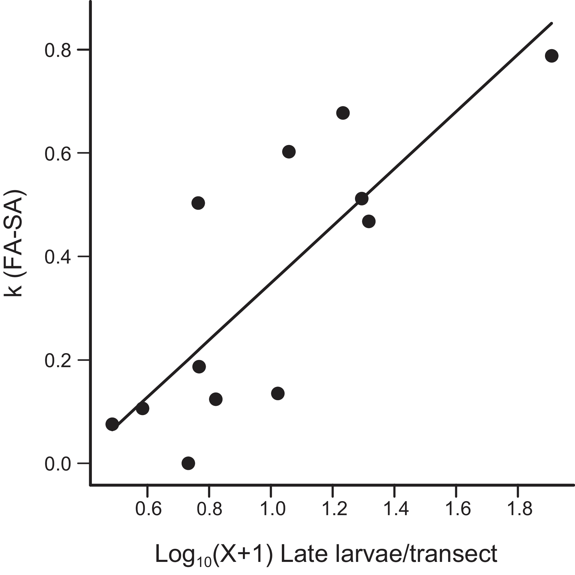
Of the regressions in which the k-values were plotted against the log densities of previous stages, the regression of k(FA − SA) on the log of late-instar larval density was significant, with a slope of 0.553 ± 0.153 (CL 95%: +0.33, +0.97; Fig. 4), as was the regression of all mortality from late-instar larvae through to spring adults (k[LL − SA] = log10[LL] − log10[SA]) on the log density of late-instar larvae (slope = 0.628 ± 0.174; CL 95%: +0.35, 1.05). Log-transformed densities of late-instar larvae and fall adults were strongly correlated (r = +0.72; df = 14; P < 0.02). None of the other regressions involving responses of k-values to densities of previous life stages was significant (P > 0.05), nor were any of the regressions of the following cohort’s k(E − LL) significant on log densities in the previous cohort.
Regression of overwintering mortality, k(FA − SA), on the log-transformed density of late-instar larvae.

Mortality and environmental variables
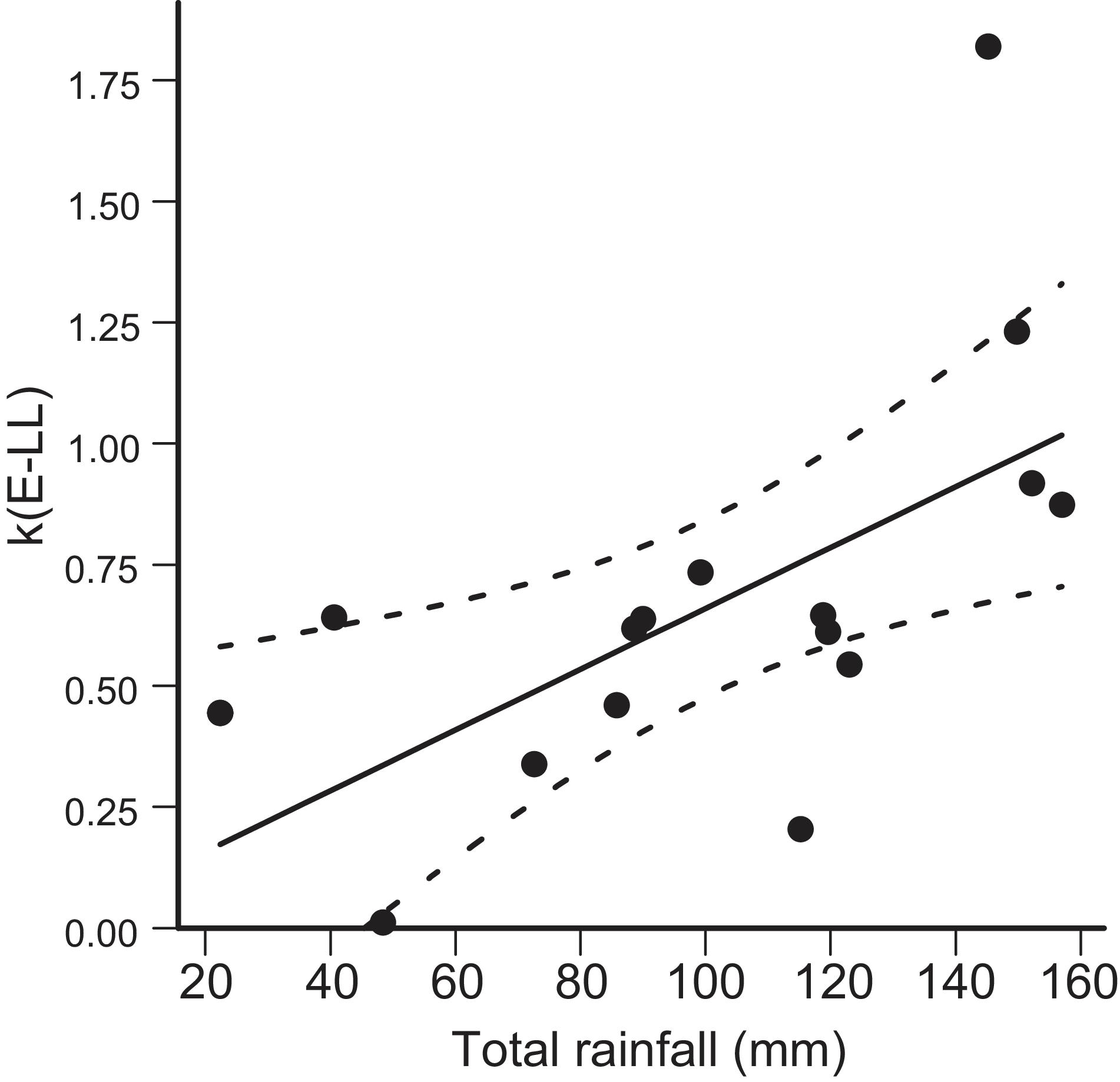
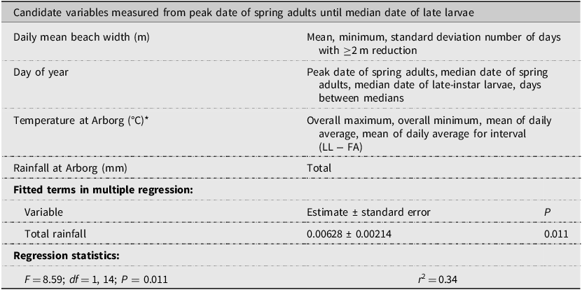
In the multiple-regression analysis of the relationships of k(E − LL), total rainfall was the only significant independent variable (Table 2). Increased rainfall was associated with increased mortality (Fig. 5), and the relationship explained 34% of the variation in k(E − LL). Among the candidate variables, there was a negative correlation of rainfall with average daily temperature (correlation coefficient, r = −0.62; df = 14; P = 0.01) and a positive correlation of rainfall with the standard deviation of daily mean beach width (r = +0.59; df = 14; P = 0.02), neither of which were included in the regression model. The relationship of rainfall to k(E − LL) is not well represented by the linear model of the multiple-regression procedure: mortalities seem relatively independent of rainfall below 130 mm; the four highest k-values occurred when rainfall exceeded 145 mm (Fig. 5).
Result of multiple-regression investigations of environmental variables associated with mortality between eggs and late-instar larvae, k(E − LL), showing the relationship between k(E − LL) and rainfall. The solid line is the fitted regression, and the dashed lines are the 95% confidence limits for the regression line.

Summary of multiple-regression analysis of the relationship between candidate environmental variables and k-values for mortality from eggs to late-instar larvae, k(E − LL).
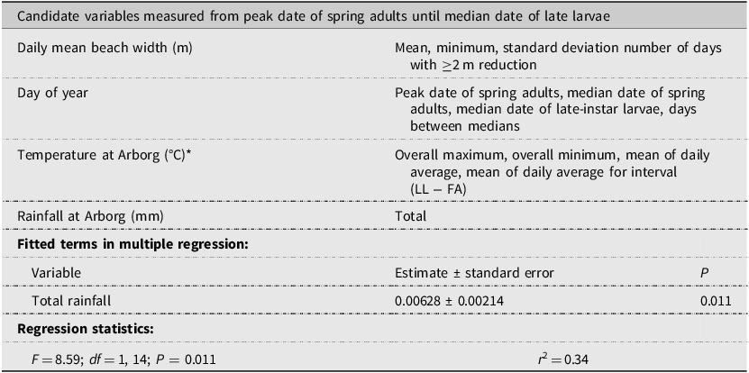
Table 2. Long description
The table presents candidate variables measured from the peak date of spring adults until the median date of late larvae. It includes daily mean beach width in meters, day of the year, temperature at Arborg in degrees Celsius, and rainfall at Arborg in millimeters. The table also lists fitted terms in multiple regression and regression statistics. The candidate variables section has four rows and two columns, detailing measurements like mean, minimum, standard deviation, and number of days with a 2-meter reduction for beach width; peak and median dates for spring adults and late-instar larvae; overall maximum, minimum, mean of daily average temperature, and mean of daily average for interval; and total rainfall. The fitted terms section has one row and three columns, showing the estimate, standard error, and P-value for total rainfall. The regression statistics section provides F-value, degrees of freedom, P-value, and R-squared value.
*Temperature records were not available for Arborg on 6 June 1990: those from Hodgson2 were used on this date instead.
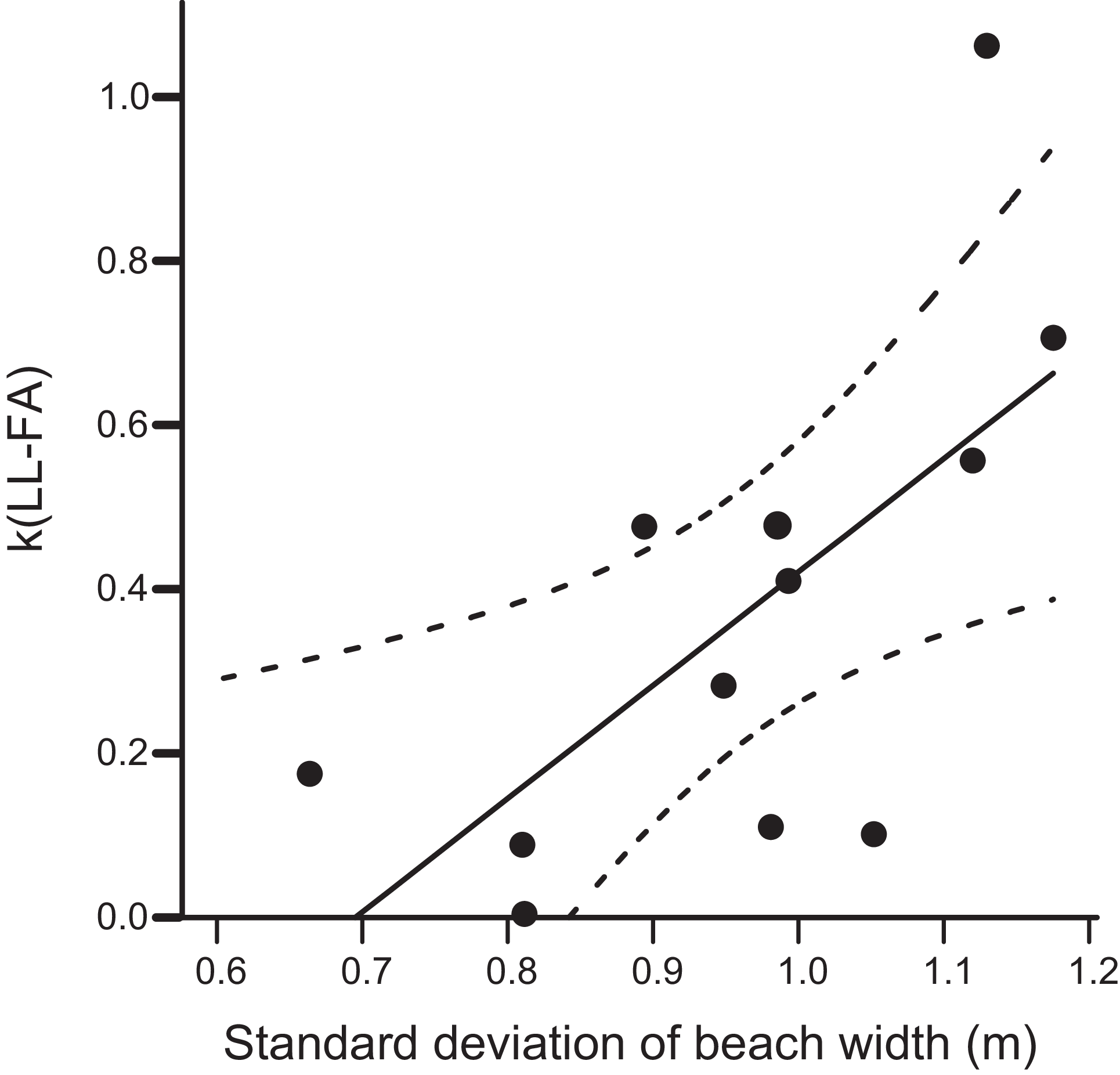
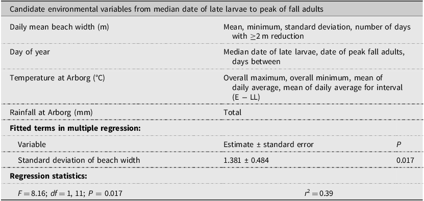
In the multiple-regression model (Table 3) for k(LL − FA), the standard deviation of daily beach width was the only significant independent variable, and the relationship explained 39% of the variance of k(LL − FA). Increased mortality is associated with increasing variability in beach width (Fig. 6). Standard deviation of beach width was not significantly correlated with any other candidate environmental variable.
Result of multiple-regression investigations of environmental variables associated with mortality between late-instar larvae and fall adults, k(LL − FA), showing the relationship between k(LL − FA) and the standard deviation of beach width. The solid line is the fitted regression, and the dashed lines are the 95% confidence limits for the regression line.

Summary of multiple-regression analysis of the relationship between candidate environmental variables and k-values for mortality from late-instar larvae to fall adults, k(LL − FA).
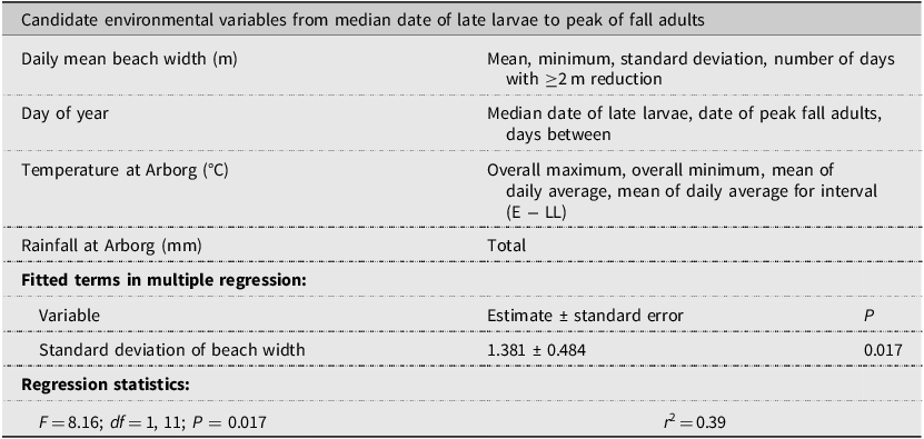
Table 3. Long description
The table presents a summary of multiple-regression analysis of the relationship between candidate environmental variables and mortality rates from late-instar larvae to fall adults. It includes four rows and three columns. The columns are labeled Candidate environmental variables from median date of late larvae to peak of fall adults, Day of year, Temperature at Arborg (degrees C), Rainfall at Arborg (mm), Fitted terms in multiple regression, and Regression statistics. The rows under Candidate environmental variables from median date of late larvae to peak of fall adults include Daily mean beach width (m), Day of year, Temperature at Arborg (degrees C), and Rainfall at Arborg (mm). The row under Fitted terms in multiple regression includes Variable, Estimate ± standard error, and P. The row under Regression statistics includes F, d.f., P, and r squared. The table provides specific values and statistical measures related to the analysis.
Note: Temperature and rainfall records were not available for Arborg for 1–19 August 1997: those for Hodgson2 were used for these dates instead.
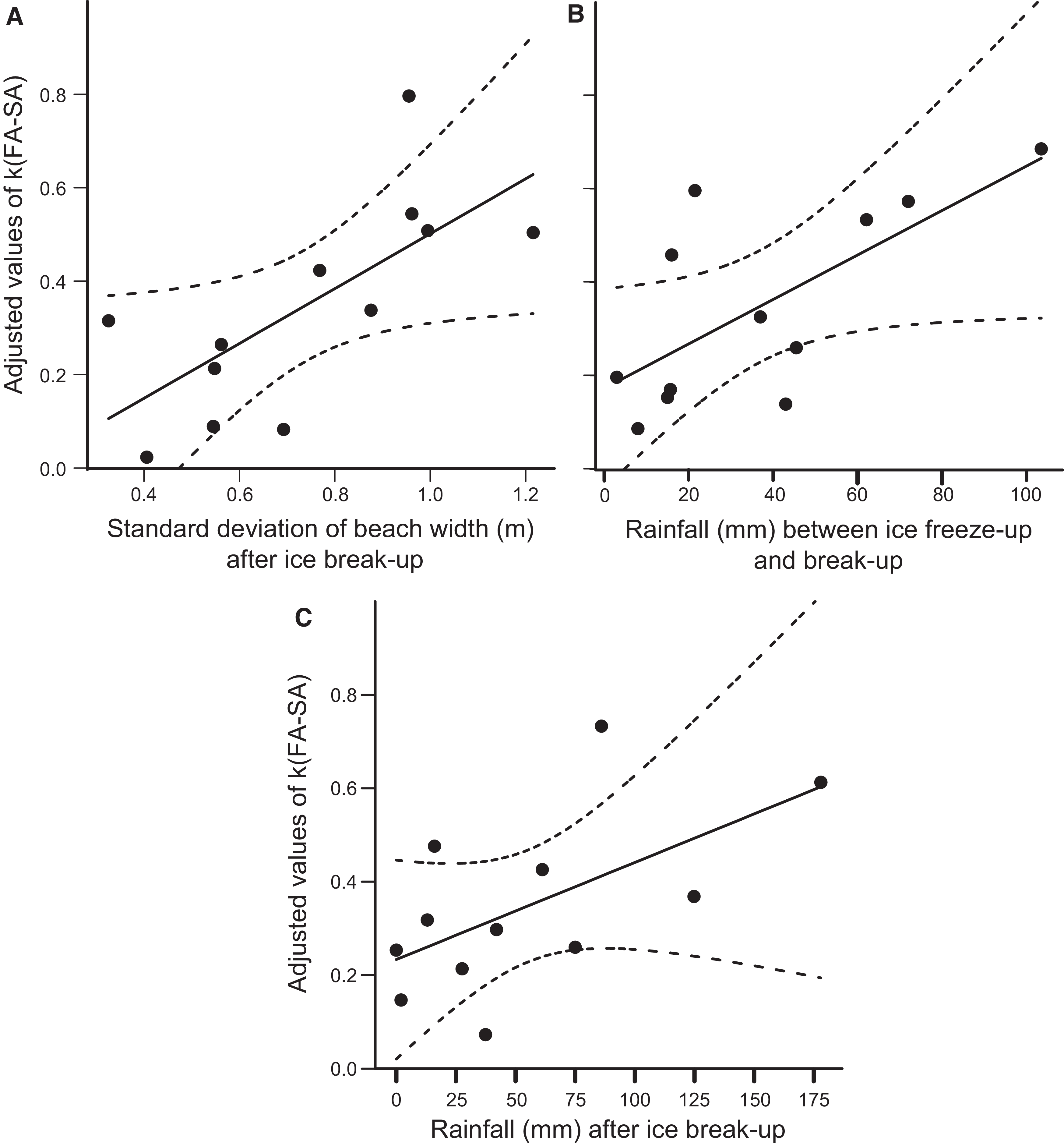
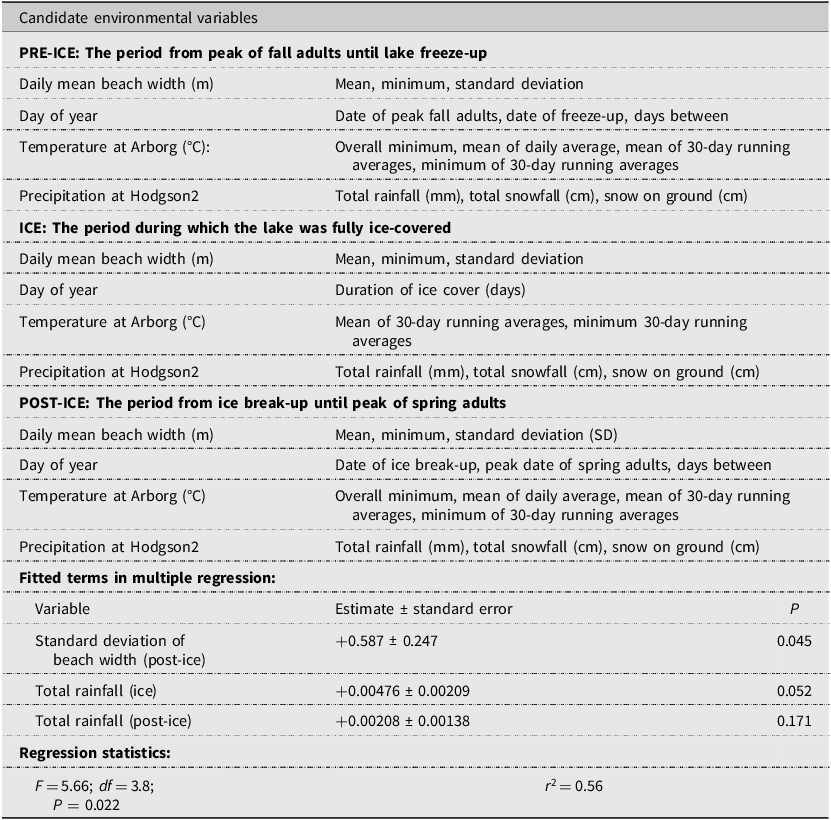
For k(FA − SA), a multiple-regression model including the standard deviation of beach width after spring ice break-up, rainfall during the period when the lake was ice-covered, and rainfall after ice break-up explained 56% of the variance (Table 4). Estimates from these three variables were not significantly correlated (P > 0.1). Increased variability of beach width in early spring was associated with higher mortality, as was increased rainfall during or after the period when the lake was frozen (Fig. 7). Of the three included independent variables, standard deviation of beach width after ice break-up was positively correlated with the 30-day running average temperature during the period that the lake was ice-covered (r = +0.66; df = 13; P = 0.03); rainfall after ice break-up was positively correlated both with average beach width before (r = +0.69; df = 13; P = 0.02) and during (r = +0.60; df = 13; P = 0.02) the period of ice cover and with the interval between the dates of ice break-up and peak numbers of spring adults (r = +0.66; df = 13; P = 0.03). None of these correlated variables was included in the regression model because none of them explained as much variance in k(FA − SA) as the correlated variables that were included in the model did.
Results of multiple-regression investigations of environmental variables associated with mortality between fall adults and spring adults, k(FA − SA): A, relationship between k(FA − SA) and standard deviation of beach width after ice break-up; B, relationship between k(FA − SA) and rainfall during the period when the lake was ice-covered; C, relationship between k(FA − SA) and rainfall after ice break-up. In each plot, values of k(FA − SA) are adjusted to remove the influence of the other variables in the regression model. The solid line is the fitted regression, and the dashed lines are the 95% confidence limits for the regression line.

Figure 7. Long description
Three scatter plots depict relationships between environmental variables and mortality rates in carabid beetles. Panel A: A scatter plot shows the relationship between the adjusted values of k(FA-–SA) and the standard deviation of beach width after ice break-up. The x-axis represents the standard deviation of beach width in meters, ranging from 0.4 to 1.2. The y-axis represents the adjusted values of k(FA-–SA), ranging from 0.0 to 0.8. The solid line is the fitted regression, and the dashed lines are the 95% confidence limits for the regression line. Panel B: A scatter plot shows the relationship between the adjusted values of k(FA-–SA) and rainfall during the period when the lake was ice-covered. The x-axis represents rainfall in millimeters, ranging from 0 to 100. The y-axis represents the adjusted values of k(FA-SA), ranging from 0.0 to 0.8. The solid line is the fitted regression, and the dashed lines are the 95% confidence limits for the regression line. Panel C: A scatter plot shows the relationship between the adjusted values of k(FA-–SA) and rainfall after ice break-up. The x-axis represents rainfall in millimeters, ranging from 0 to 175. The y-axis represents the adjusted values of k(FA-SA), ranging from 0.0 to 0.8. The solid line is the fitted regression, and the dashed lines are the 95% confidence limits for the regression line.
Summary of multiple-regression analysis of relationship between candidate environmental variables and k-values for mortality between the peak densities of fall adults and spring adults, k(FA − SA).
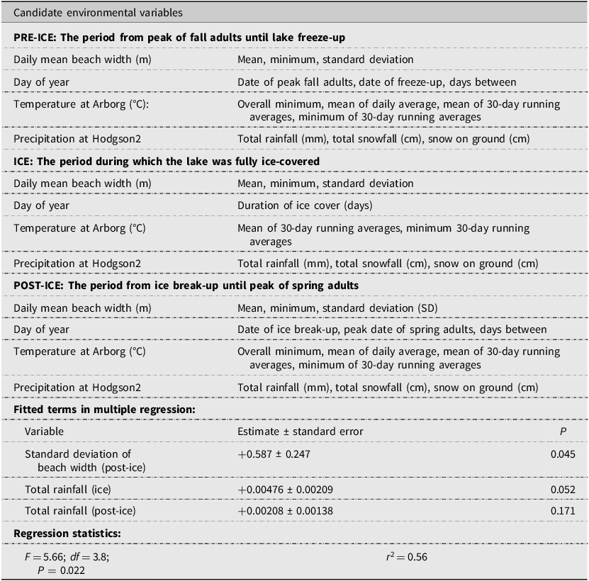
Table 4. Long description
A table comparing candidate environmental variables and their impact on mortality rates. The table has 15 rows and 4 columns. Column headers are Candidate environmental variables, PRE-ICE, ICE, and POST-ICE. Row labels include Daily mean beach width (m), Day of year, Temperature at Arborg (°C), Precipitation at Hodgson, Fitted terms in multiple regression, and Regression statistics. The table lists various environmental variables measured during different periods and their respective mean, minimum, standard deviation, and other relevant statistics. It also includes estimates, standard errors, and P-values for fitted terms in multiple regression, along with regression statistics such as F-value, degrees of freedom, P-value, and r-squared value.
Note: Temperature records were unavailable for Arborg on the following dates, and temperatures for Hodgson2 were used instead: 7–12 November 1984, 11 November 1985, 10–17 March 1993, and 1–21 May 1994.
Discussion
The sample universe for this population was part of a continuum of stony beaches along which sampling was performed. Immediately north and south of the sample universe were similar areas of beach that appeared to have similar numbers of C. cordicollis. It is certain that some interchange by walking occurred at the boundaries of the sample universe, but it is assumed that the interchange was bidirectional and therefore probably did not produce significant change in the numbers in the sample universe. Beetles were never found in intensive searches and pitfall trapping on the lower slopes or on the crest of the beach-top cliff (unpublished data), suggesting that C. cordicollis is confined to the beach habitat. Movement to beach-top overwintering sites effectively removes adult beetles from the sampling universe, because beetles are not recovered in transect samples when in overwintering sites (Holliday Reference Holliday2025a). However, it seems reasonable to assume that beetles that leave the sampling universe in the fall and survive winter return to the sample universe in the spring. Dispersal by flight may occur shortly before the reproductive season, but the flight period follows closely after ice break-up, so in many years, flight is possible on few or no days because air temperatures are below the threshold for flight (Holliday Reference Holliday2025b).
Samples in May and early June typically showed an increasing trend as adults were recruited from beach-top overwintering sites. In many – but not all – years, there followed a period of relatively similar densities, suggesting that, in those years, mortality was not significantly depleting the population at this time. Subsequently, densities of adults declined, and late-instar larval densities increased; the adult decline is likely due to postreproductive mortality because overwintered adults do not survive after reproduction (Holliday et al. Reference Holliday, Mattingly, Toro, Donald and Holliday2016). The estimates of peak densities of spring adults, lying as they do between the time of recruitment from overwintering sites and the postreproductive decline, are probably reliable estimates of densities of adults surviving winter and becoming reproductive.
Estimates of densities of eggs depend on the estimated number of spring females and the average number of eggs per gravid female determined by dissection. In the laboratory, females mature large numbers of eggs and have distended abdomens before beginning oviposition; after oviposition begins, females rapidly become less distended (Holliday Reference Holliday2025a). There is no evidence of additional eggs being developed (unpublished data), and so it is assumed that the number of eggs in fully gravid females adequately estimates fecundity. For Pterostichus madidus (Fabricius) (Coleoptera: Carabidae) and Harpalus aeneus (Fabricius) (Coleoptera: Carabidae), the average maximum egg content of females is very similar to the total number of eggs laid per female (Luff Reference Luff1982), but this is not so in Pterostichus caerulescens (Linnaeus) (Coleoptera: Carabidae) and Calathus melanocephalus (Linnaeus) (Coleoptera: Carabidae) (van Dijk Reference van Dijk, den Boer, Thiele and Weber1979).
Reproductive development is initiated in response to photoperiod and, in years when not delayed by late ice break-up, 50% of females are expected to be fully gravid on 10 June (Holliday Reference Holliday2025a). At average July temperatures, the interval from oviposition to the beginning of the third larval instar is about 19 days (Holliday Reference Holliday2025a), but eggs and larvae in June would typically experience cooler temperatures that would be expected to slow development, an expectation that is supported by the relationship of June temperatures with the peak date for late-instar larvae. Temperature would also affect the duration of the late-instar larval stage that is detectable in quadrat samples. Warmer temperatures would shorten that duration, which would result in the method of Southwood and Jepson (Reference Southwood and Jepson1962) underestimating the number passing through the late-instar larval stage. Strong temperature dependence of the estimate of late-instar larvae could influence values of k(E − LL) and k(LL − FA). Temperatures during these two intervals were candidates in the analyses of the association of environmental variables with k-values, but for neither interval was a significant effect observed. So, it may be concluded that temperature-related errors in estimation of numbers of late-instar larvae did not greatly influence analyses.
Holliday et al. (Reference Holliday, Mattingly, Toro, Donald and Holliday2016) concluded that, in Manitoba, adult C. cordicollis die after reproduction. New-generation beetles remain teneral, with soft and highly iridescent elytra for 2–3 weeks after eclosion (Holliday Reference Holliday2025a), and are readily distinguishable from overwintered beetles, which are dull from abrasion with their stony habitat. In addition, the amount of 2,3-dimethylphenol in the defensive secretion of adult beetles declines exponentially with time since eclosion and so can be used to assess adult age. Discriminant analysis using the amount of 2,3-dimethylphenol was 97% accurate in determining the generational status of beetles and confirmed that, in three years of sampling in Manitoba, there were no overwintered beetles in samples after 24 August (Holliday et al. Reference Holliday, Mattingly, Toro, Donald and Holliday2016). Population patterns observed in the current study are consistent with the conclusion that postreproductive beetles do not survive to reproduce again: in three of the 16 years, there was a period of at least 15 days in mid-summer in which no adult beetles were collected, suggesting that collections after that interval were entirely new-generation beetles.
Peak adult densities following the larval peak were considered to represent new-generation fall adults; however, the pattern of fall adults varied considerably among years, with the date of peak fall adult density occurring any time between early August and late September. In years without a mid-summer period with no adults in samples, surviving spring adults may have been present after the larval peak and could result in an overestimation of fall adults when the peak for “fall adults” was early. In September, beetles are found nearer the top of the beach than they are from June to August (Holliday Reference Holliday2025a), and it is probable that movement to overwintering sites begins earlier than the downturn in density that was seen in most years in September. Based on this, there may be years when peak fall adults is an underestimate because not all fall adults are available for sampling at any one time: some have moved to overwintering sites and others have not yet completed pupal eclosion. In mark–recapture studies, dispersal of adults in August and September averaged 2.5 m/day, which was higher than in spring (unpublished data), and may also have contributed to the variability of estimates of peak fall adults. These uncertainties suggest that estimates of fall-adult densities are less reliable than are estimates for other stages and likely account for the negative k-values and the greater range of annual density estimates than are shown by other stages.
Although average net reproductive rates, R 0, did not indicate a trend for population growth over the course of the present study, the maximum values of R 0 indicated that the populations of late-instar larvae and of spring adults had the capacity to increase 7.7-fold per generation under favourable conditions. Therefore, in the absence of regulatory processes, a succession of two generations under favourable conditions could result in a 60-fold population increase – a much larger increase than was observed in the present study. Hassell (Reference Hassell1986) argued that the absence of unbounded growth in populations is evidence for the universality of some form of density-dependent regulation, but that author acknowledged that detecting density-dependent processes is challenging. The noted carabid ecologist P.J. den Boer vigorously disputed the pervasiveness of density dependence (e.g., den Boer Reference den Boer1990) and favoured mechanisms involving spreading of risk (den Boer Reference den Boer1968).
The key mortality factor responsible for population change in the present study was k(E − LL), mortality in the stages between eggs and late-instar larvae. Mortality of larvae is considered a key factor in population dynamics of many carabid species, and cannibalism among larvae is common (Lövei and Sunderland Reference Lövei and Sunderland1996; Luff Reference Luff, Lövei and Toft2005). In Pterostichus oblongopunctatus (Fabricius) (Coleoptera: Carabidae), larval cannibalism is an important contributor to density regulation (Heessen and Brunsting Reference Heessen and Brunsting1981). However, some species of Chlaenius do not exhibit larval cannibalism (Zetto Brandmayr et al. Reference Zetto Brandmayr, Bonacci, Massolo and Brandmayr2004), and C. cordicollis larvae are not aggressively cannibalistic, given that they can be successfully reared in groups in simple beach-like microcosms (Holliday et al. Reference Holliday, Mattingly and Holliday2015). Because k(E − LL) is not density-dependent, there is no evidence that larval cannibalism is an important source of mortality in the study population.
Mortality k(E − LL) was significantly related to rainfall, and the four highest k-values for mortality were all associated with total rainfall of more than 145 mm during the interval between the peak of spring adults and the median date of occurrence of late-instar larvae. The 1990 cohort suffered almost 99% mortality during this stage; 75 mm of rain fell in the first 12 days of June 1990 (Environment Canada 2025b), a time when the majority of the study population would be eggs or first-instar larvae (Holliday Reference Holliday2025a). In the other years with high rainfall, mortality was somewhat less than in 1990, and the rainfall was more dispersed throughout the egg and young-larval period. Excessive moisture increases immature mortality in other carabid beetles. For example, soil moisture content above 20% reduces larval survival in Poecilus cupreus (Linnaeus) (Coleoptera: Carabidae), and no larvae survive 60% soil moisture (Theiss and Heimbach Reference Theiss and Heimbach1994); also, high moisture levels increase larval mortality of Pterostichus oblongopunctatus (Fabricius) (Coleoptera: Carabidae) (den Boer et al. Reference den Boer, Szyszko and Vermeullen1993). Eggs survived flooding in laboratory studies of the riparian beetle, Bembidion velox (Linnaeus) (Coleoptera: Carabidae) and, at substrate moisture contents of 5–11%, larval mortality was 20–30%; however, larval mortality was 50–75% at a minimum of 25% moisture, with most mortality occurring in the first instar (Kleinwächter and Bürkel Reference Kleinwächter and Bürkel2008).
Mortality k(LL − FA) was significantly associated with variability in beach width. The highest mortality occurred in 1991, when, in the period between the median date of late-instar larvae and the peak of fall adults, there were five occasions when daily mean beach width diminished by more than 2 m over a 24-hour period, with a maximum daily reduction of 3.3 m and a two-day event when beach width declined by 4.8 m (Environment Canada 2024). Because changes in water content of the south basin of Lake Winnipeg occur over a time scale of months not days, these fluctuations are the result of wind-driven seiches, to which Lake Winnipeg is prone (Einarson and Lowe Reference Einarson and Lowe1968). The daily mean beach width is based on the 24-hour average lake level and so does not capture either short-term minima in beach width or the effects of waves, which would normally be high if the seiche was driven by onshore winds on the east-facing beach. Because lethargic third-instar larvae, pupae, and newly eclosed teneral adults have limited or no mobility (Holliday Reference Holliday2025a), they would be either immersed and drown if they were close to the waterline at the onset of a seiche or crushed by the wave-agitated movement of beach stones.
No significant association of mortality k(FA − SA) with variability of beach width before freeze-up was observed, probably because adults are located high on the beach in fall (Holliday Reference Holliday2025a). However, after spring ice break-up, greater variability of beach width was found to be associated with greater mortality. In early spring, air temperatures adjacent to the recently thawed lake are much lower than they are further inland (Holliday Reference Holliday2025b): in the first half of May, lakeside average temperatures are 7.5 °C and average overnight minima are 3.1 °C; in the second half of the month, corresponding averages are 16.2 °C and 7.8 °C (Environment Canada 2025d). As agility and walking speed of C. cordicollis adults decline steeply at temperatures below 10 °C (Holliday Reference Holliday2025a), ability to escape an early spring seiche would be impaired. Mortality also increased during years with higher total rainfall after ice break-up. As rainfall did not affect mortality in the period before the peak of fall adults, it is not clear how rainfall affects adult survival.
Rainfall can occur in winter during warm episodes between periods when air temperatures below −20 °C are common. Larger amounts of rainfall while there was ice on the lake were associated with increased mortality k(FA − SA). Once ice covers the lake, snow can blow off the ice and accumulate in drifts over C. cordicollis overwintering sites. The drifts provide insulation, resulting in temperatures at overwintering sites that are higher than those elsewhere on the beach; these warmer microclimates are critical to the overwintering survival of C. cordicollis, which is intolerant of temperatures below approximately −7 °C (Holliday Reference Holliday2025a). Rainfall on snow transfers heat to the snowpack both because the rain is above 0 °C and because the rain freezes releasing latent heat of fusion (Marchand Reference Marchand2013); consequences include changes in snow crystal structure, formation of ice layers, and reduced insulating capacity of the snow. Therefore, if substantial rainfall occurs and is not immediately followed by fresh insulating snow, temperatures in overwintering sites may drop below C. cordicollis’s range of tolerance.
Abiotic influences are considered the principal mortality factors for carabid beetles (Lövei and Sunderland Reference Lövei and Sunderland1996); in the current study, only abiotic factors were studied because field investigations of natural enemies and competition are problematic in an environment where enclosures are difficult to establish in the stony substrate and can be overwhelmed by seiches or ice. However, abiotic mechanisms are unlikely to account for density dependence of mortality, which usually involves biotic processes, such as competition for resources or effects of natural enemies (Hassell Reference Hassell1986).
Overwintering mortality, k(FA − SA), was dependent on the mutually correlated densities of fall adults and late-instar larvae. As all mortality from late-instar larvae to spring adults, k(LL − SA), was also dependent on density of late-instar larvae, the density dependence was not a result of unreliability in estimates of density of fall adults. The slopes of the regressions indicating density dependence were less than 1, which signifies that the effect of the mortality would be undercompensating regulation of population density (Varley et al. Reference Varley, Gradwell and Hassell1973).
The density dependence of overwintering mortality appears unlikely to be attributable to competition or predation in overwintering sites. Overwintering beetles are often found in aggregations of more than 100 individuals (Holliday Reference Holliday2025a), so there are unlikely to be disadvantages to locally high densities in suitable sites. Indeed, aggregation of chemically defended adults is thought to provide enhanced protection from predators (Bonacci et al. Reference Bonacci, Mazzei, Zetto Brandmayr and Brandmayr2004; Zetto Brandmayr et al. Reference Zetto Brandmayr, Bonacci, Massolo and Brandmayr2006). The phenolic pygidial defensive secretions of C. cordicollis deter ants, lizards (Eisner et al. Reference Eisner, Hurst and Meinwald1963), and frogs (unpublished data), all of which are common potential predators in the summer but, as ectotherms, are probably not a threat to overwintering beetles. No evidence was seen of predators excavating overwintering aggregations (unpublished data). The prevalence of parasitic nematodes and fungi is low in gravelly or stony riparian habitats (Andersen and Skorping Reference Andersen and Skorping1991), and they were not detected during dissections of C. cordicollis larvae or adults. In numerous laboratory rearings of field-collected adults, parasitoids such as Euphorinae that emerge from adult Carabidae (Loan and Holliday Reference Loan and Holliday1979) were not detected (unpublished data). Based on this, competition and natural enemy impacts while beetles are in overwintering sites appear improbable, and the beetles’ chemical defences are likely to deter predators both before and after they are in overwintering aggregations. Therefore, the mechanism of density dependence probably involves competition for a limiting resource before entry into the overwintering sites.
A likely mechanism of density dependence is that some of the adults entering overwintering sites have insufficient metabolic reserves for them to survive the 7–8 months until they can feed in spring. Competition for food could be restricted to the few weeks between pupal eclosion of fall adults and their entry into overwintering aggregations. Shortly after eclosion, fall adults move to the top of the beach, located beyond the reach of most seiches at a time when temperatures may be too low for the beetles to flee them (Holliday Reference Holliday2025a). However, beetles at the top of the beach are distant from their major food source of dead or dying insects washed ashore by the lake (Larochelle and Larivière Reference Larochelle and Larivière2003; Holliday Reference Holliday2025a), and the less abundant food sources near the top of the beach could be depleted when densities of fall adults are high. There may be additional influences of competition for food among larvae if, as in N. brevicollis (Nelemans Reference Nelemans1987), there are long-term effects of larval nutrition. That k(LL − FA) was independent of larval density suggests that larval competition for food is not severe enough to cause mortality before the peak of fall adults. However, feeding by fall adults may not be able to compensate for preexisting stress caused by competition between larvae for food. Because larval and fall adult densities are correlated, it is not possible to determine whether competition occurs at only one stage or at both stages.
Conclusions
The ability to sample multiple stages of C. cordicollis quantitatively in the variable environment of a stony beach made it possible to develop the first published series of budgets – stage-specific life tables – for a carabid beetle. The series provided evidence that, as in many carabid species, early juvenile mortality is the key mortality factor, and that high mortality at this stage is associated with high rainfall. Short-term variations in beach width during wind-driven seiches that rapidly raise lake levels are associated with mortality of stages that have limited mobility, including larvae about to pupate, pupae, newly emerged teneral adults, and adults in early spring when cool temperatures inhibit rapid movement. Contributing to winter mortality is the reduced insulating capacity of snow drifts covering the beetles’ overwintering sites that occurs when rain falls on the snow. Overwintering mortality is density-dependent, which seems likely to be a consequence of competition for food by fall adults, larvae, or both, resulting in some beetles entering wintering sites with insufficient metabolic reserves to survive until spring.
Acknowledgements
Technical assistance was provided by D. Holder, D. Wright, S. Heuchert, G. Marino, L. Klymochko, L. Donald, and numerous summer student assistants. R. Lamb and L. Donald provided valuable critiques of an early draft of the manuscript. Funding was provided by the Natural Sciences and Engineering Research Council of Canada and the University of Manitoba. Permission to work in the study site was granted by Manitoba Environment and Climate Change.
Competing interests
The author declares no competing interests.


 Open access

