1. Introduction
Fishing effort, as measured by the number of fishing days for a given trip, is probably one of the most important decisions for any fisherman. Studies on fishing effort have been widely published. To the best of our knowledge, most of these studies use the standard assumptions of economic theory, namely that economic agents are rational and self-interested. In this paper, we explore the fishermen's decision-making behavior on the number of fishing days per trip by applying an alternative framework using the target revenue model.Footnote 1 We will see how having a target revenueFootnote 2 may influence the fishermen's decision regarding trip length and how this may result in a different prediction from the standard economic model regarding the relationship between daily fishing revenue and the number of fishing days. To investigate which model provides a more reasonable description of reality, we observe the empirical evidence from the Hawaii-based longline fisheries.
Regarding the literature on labor supply, the question of how much workers respond to change in wages is fundamental. Recent studies have moved towards analyzing an alternative determinant of labor supply hypothesis that deviates from the conventional framework: reference-dependent preferences (see Kahneman and Tversky, Reference Kahneman and Tversky2000 for a selection of papers on this topic). With such preferences, an individual's utility for any given period depends on an income target: if income falls below this target, then the worker's marginal utility of income is higher than if income is above the target. Hence, a temporary increase in earnings may (but not necessarily) lower labor supply because the desired reference-income can then be achieved with less work effort.
There are factors that make fisheries an interesting case study. First, anecdotal evidence seems to suggest that fishermen may exhibit income-targeting behavior (Lynham et al., Reference Lynham, Siegel and Costello2007; Holland, Reference Holland2008). However, there has been no empirical study to investigate this evidence. Second, fishermen face capacity constraints for fuel and food supplies. These constraints may result in shortening the trip despite not having achieved the target revenue goal for a given trip as predicted by the target revenue model. Third, Hawaii-based longline fisheries consist of owners from different ethnic groups, each one potentially behaving differently in the decision-making process. Accordingly, certain groups of owners may be more likely to behave in accordance with the standard economic model, whereas others are more likely to behave according to the target revenue model. Finally, Hawaii's longline fishermen generally vary in terms of fishing experience, which allows for estimation of correlation between experience and observed behavior.
As far as fishery management is concerned, the idea that fishermen seek target revenue could have important policy implications. First, to achieve the target the fishermen may be willing to make risky and unsafe decisions. For instance, due to stormy conditions, it may take longer for the vessel to achieve the target. Thus, the captain may be willing to prolong the trip rather than return to port despite the storm. That decision would threaten the lives of the whole crew. Likewise, the fishermen may be willing to take the risk of being fined so they can fish in a restricted area in order to achieve the preset target. Along this line, Holland (Reference Holland2008) suggests that fishery management officials may consider two alternatives in establishing compliance strategies: policies with high probability of detection and moderate fine, or policies with low probability of detection and high fine.
Another relevant aspect of revenue targeting in fishery management relates to a popular policy experiment aimed at preventing further entry and rebuilding the stock once the fishing stock reaches a steady state. Given this scenario, Lynham et al. (Reference Lynham, Siegel and Costello2007), using a simulation model, show that in a fishery which includes both income maximizers and income targeters, incumbent fishermen would not be better off by closing the fishery and rebuilding the stock. Accordingly, fishermen rarely support such a policy proposal (Lynham et al., Reference Lynham, Siegel and Costello2007).
We proceed with the remainder of the paper as follows. In the next section, we discuss the literature which has a special focus on the target revenue model in fisheries. We then present a simple target revenue model in a fishery. Next, we investigate the following questions: (1) how well does the target revenue model describe the fishing behavior of Hawaii's longline fishermen? and (2) how do capacity constraints impact fishermen's behavior under the target revenue model framework? We then conclude the paper.
2. A literature review
A great number of recent studies on labor supply have followed the intertemporal formulation of the standard neoclassical model (Camerer et al., Reference Camerer, Babcock, Loewenstein and Thaler1997; Chou, Reference Chou2002; Farber, Reference Farber2005). The model predicts, under the standard framework, that there is a positive correlation between the number of working hours and wage rate.
Studies on the supply of labor have empirically shown little support for the standard model's prediction. Although most studies have found a positive correlation between labor wages and labor supply, the results are not significant. This insignificant relationship found in the empirical studies can be attributed to a number of factors. For instance, in many settings workers are required to work a fixed number of hours per day regardless of their hourly wage. Another question is whether changes in wages are temporary or permanent with respect to the time horizon of the decision-making framework. Under the standard model of labor supply, decisions are made under a long-run or lifelong horizon.
Most empirical studies in fisheries, however, assume that decision making is short term (i.e., a fishing trip). This short-run time horizon, for example, certainly impacts on the standard model's predictions of fishermen's behavior (Eggert and Lokina, Reference Eggert and Lokina2007). In a seminal paper to describe the labor supply behavior of fishery captains, Gautam et al. (Reference Gautam, Strand and Kirkley1996) develop a model that highlights both contemporaneous and intertemporal trade-offs between labor and leisure. They then test the theory based on data from a sea-scallop fishery. The key finding is that the short-run labor supply exhibits a backward-bending property. More specifically, captains were found to increase time at sea and decrease time onshore in response to higher current-period profits per day. At sufficiently high levels of profits per day, captains reduce time at sea and increase time onshore. The findings suggest that labor supply is backward bending in current daily profits, whereas leisure demand is forward falling.
In the search for a model to bridge the gap between theoretical prediction and empirical evidence, increasing attention has been paid to the target revenue model, which offers an alternative description of labor supply. In what follows, we will briefly review the labor supply studies based on the target revenue model.
2.1. Revenue target model: a prospect theory-based model
The seminal paper by Camerer et al. (Reference Camerer, Babcock, Loewenstein and Thaler1997) on the labor supply of taxi drivers in New York City is the first study on labor supply under the prospect theory framework. Camerer and colleagues find a negative elasticity for the taxi drivers’ working hours with respect to hourly wage in the range of [−0.61, −0.18]. According to the authors, the negative relationship between the number of working hours and average wage rate results from the fact that each taxi driver has a daily target income level. On a given day, drivers continue driving until they achieve their target income levels. On a productive day with many customers, it takes only a few hours to meet that target goal. Conversely, on days with fewer customers, it takes more hours to reach that same target level.
Following Camerer et al.’s paper, numerous researchers have conducted labor supply studies based on the target revenue model. Using a similar approach, Chou (Reference Chou2002) finds that Singaporean cab drivers exhibit exactly the same decision-making behavior on time allocation as those in New York City. Fehr and Goette (Reference Fehr and Goette2007) provide an innovative method to conduct a labor supply study. They use a randomized field experiment to explore how bike messengers respond to changes in hourly wages. They estimate the loss aversion parameters of the participants and find that messengers with strong loss aversion behaved in accordance with the target revenue model. Conversely, messengers with less loss aversion appear to follow the standard model of labor supply, i.e., they increase effort levels in response to an increase in the piece rate.
In support of the standard intertemporal model, Farber (Reference Farber2005, Reference Farber2008) also conducts a study on New York taxi drivers. Farber's approach focuses on the probability of continuing to drive at any given time by asserting that the greater the number of accumulated driving hours, the lower the probability that a driver will continue to drive. He argues that the key factor in determining the cab driver's daily driving hours is the number of hours driven. Farber finds a positive but not significant effect of cumulative earning on the probability of stopping driving. This finding is qualitatively consistent with the target income model. Farber also finds a significant and positive impact of cumulative working hours on the probability of stopping which gives support for the standard model of labor supply.
The most recent study by Crawford and Meng (Reference Crawford and Meng2011) offers a convincing reason for the validity of the target revenue model despite Farber's finding. Based on the framework of expectation-based reference-dependent preferences developed by Köszegi and Rabin (Reference Köszegi and Rabin2006), Crawford and Meng argue that, as the workers work longer than the targeted hours, they also experience loss as income is below the income target level. Crawford and Meng use the same set of data and apply the same structural model approach as that utilized by Farber. The important distinction is that they consider targets as the agent's rational expectations rather than the latent variables as Farber does. More specifically, Crawford and Meng use the average of realized incomes and working hours as a proxy for the targets. Their main finding is that the probability of stopping work is determined by income when the realized income is higher than expected as supported by Camerer et al.'s study. When the realized income is less than expected, the probability is determined by the number of worked hours as shown by Farber. In either case the agents are likely to behave according to the target revenue model.
2.2. Target revenue model in the context of fisheries
How relevant is the target revenue model to fisheries? As discussed above, the target revenue model is drawn from a literature in which an individual (taxi driver) makes optimizing choices that are self-interested. The decision-making process in a fisheries context is rather more complicated. Most fishing vessels, including those in the longline fishery, employ three kinds of labor: owner, captain and crew. However, in the context of this study (Hawaii's longline fishery), the decision of whether to continue fishing or return to port is made by the owner and captain.Footnote 3 Like Gautam et al. (Reference Gautam, Strand and Kirkley1996), we assume that to remain employed, captains make the same choices that owners would have made. Put differently, we can think of a vessel owner/captain as an individual decision maker just like a taxi driver.
The main reason that allows fisheries to serve as an ideal application for the target revenue model is probably the short time horizon of the decision-making process and the uncertainties surrounding each trip. Decisions on the length of a fishing trip are made one trip at a time. This short time horizon differs from the standard model's assumption of using a lifelong horizon. There is also a great deal of uncertainty surrounding each trip, as it is possible that a vessel can have a highly profitable trip followed by a very unprofitable trip, and the reasons may be due to uncontrollable factors such as bad weather or poor fishing grounds. For these reasons, it is not easy for a vessel operator to expect a certain return for each fishing trip and, thus, the operator also will not know how long each trip will last. A possible strategy for the vessel operator is to establish a target revenue goal. This goal acts as a reference point to help decide whether to continue the fishing trip or not.
From interviews with vessel operators in Hawaii's longline fisheries, we found that a majority of vessel operators have a mentally constructed target revenue goal for each fishing trip. The target revenue is typically the vessel's average trip revenue realized in previous years. For example, operators of average size longline vessels mentioned aiming for a revenue of $20,000 per trip. Once the operator has reached this goal, he will very likely conclude the trip and return home. The probability of continuing the fishing trip after achieving $19,000 is much greater than continuing after receiving $21,000 of revenue. Psychologically, it is true that people are more likely to work harder prior to reaching a goal than after exceeding that goal (Fehr and Falk, Reference Fehr and Falk2002). Following the insight of Goette et al. (Reference Goette, Huffman and Fehr2004), we can say that this type of decision-making behavior makes the Kahneman–Tversky prospect theory a relevant framework in our study.
There are also other features that make fisheries an interesting case for the study of labor supply under the target revenue model. First, fishermen have the flexibility to choose their work schedules (Gautam et al., Reference Gautam, Strand and Kirkley1996), which in turn allows for variability in the number of fishing days between trips and vessels. Variation in the number of fishing days makes it possible to use trip length as the dependent variable. Second, a typical feature of decision making in the longline fishery is to consider each fishing trip in isolation. If the vessel operator made decisions based on two trips as opposed to one, for instance, the additional revenue from one productive trip could offset the loss in the other unproductive trip. In order to reach the revenue target for the two trips, the vessel operator may fish longer during the productive trip and shorter during the unproductive trip. Despite having a revenue target (for the two trips together), the vessel operator's behavior follows suit with the intertemporal model of labor supply.
2.3. Other considerations
In general, the fishing trip length decision is complex due to a number of factors, including vessel capacity and auction fish prices. A vessel's physical capacity determines the length of time that the vessel can fish. The ability to produce ice during a trip is crucial in lengthening the amount of time a vessel is out at sea. Fish price, which is controlled by market supply and demand forces, can directly impact trip revenue and induce uncertainty regarding trip length. Fish prices are determined by a high level of competition at the local United Fishing Agency fish auction and are also influenced by the number of fishing boats choosing to offload on a particular day. Depending on the number of boats offloading to the fish auction, vessel operators may gamble by shortening a trip and catching fewer pieces of fish, and offloading on a day when fewer boats are at the auction in hopes of securing higher prices to compensate for the lower quantity in fish pieces.
This paper greatly simplifies the complex process above by assuming that the vessel operator has a revenue target, as opposed to a target quantity of fish pieces caught. This assumption may cause one to ask how the vessel operator can estimate the accumulated revenue of the trip, especially when the auction fish price fluctuates on a daily basis. This is possible thanks to the constant communication between the captain who is monitoring the boat in the ocean and the owner who closely follows what is happening at the auction. Focusing solely on revenue rather than on fish prices will significantly simplify this complex price mechanism. Regarding the vessel's physical constraint to stay longer in the ocean, we use icemaker and vessel size as a proxy for vessel capacity. Having an icemaker enables larger and typically shallow-set vessels to fish longer, as does being a larger vessel. When fish are placed in an ice hold and regularly repacked to maintain a desired level of freshness over the course of many weeks out at sea, ice will melt and will have to be replaced by fresh ice from an icemaker. Otherwise, there exists a trade-off between the fish quality and the trip length.
3. A revenue target model in fishery
Our primary interest is in seeing how having a target revenue goal impacts trip length. Decisions on trip length are made one trip at a time rather than over an entire lifecycle. Hence, our model is based on a single trip. To incorporate revenue targeting, we build upon Farber (Reference Farber2008) to assume that the captain's preference takes the following form:
 $$U\lpar w\comma \; d\rpar = \left\{\matrix{\lpar wd - T\rpar - \displaystyle{{\theta}\over{1+\gamma}}d^{1 + \gamma}\hfill & \hbox{if} \, \lpar wd \gt T\rpar \cr \lambda\lpar wd - T\rpar - \displaystyle{{\theta}\over{1+\gamma}}d^{1 + \gamma} & \quad \hbox{if} \, \lpar wd \gt T\rpar }\right.$$
where U(w, d) is the utility function under prospect theory, d is the number of fishing days and w is the average daily fish revenue. T is the reference (target) revenue level. λ is a parameter representing how sensitive the captain is to deviation from the reference revenue. We assume λ > 1 to reflect loss aversion. θ is a parameter for the disutility of fishing effort (θ > 0). γ is the inverse elasticity parameter of revenue with respect to fishing days (γ > 0).
There are two elements in the utility function. The first element represents utility, which varies depending on how much the actual fishing revenue exceeds the target (wd − T). The second element is the standard disutility function. The utility function is kinked at wd = T. When the captain achieves a catch revenue exceeding the target (wd > T), the marginal utility is 1, which implies that a revenue increase of $1 results in a 1 unit increase in utility. When the captain has not achieved the target revenue level (wd < T), the marginal utility is λ, which is greater than 1, which implies that a revenue increase of $1 leads to more than a 1-unit increase in utility. In this case, the captain places more value on a $1 revenue increase because the captain has yet to reach the point where wd = T and, thus, is more willing to continue fishing. A productive fishing trip shortens the time in which the captain can achieve the target goal (i.e., wd > T), whereas an unproductive trip lengthens the time the captain has to achieve the target goal as there is incentive to fish longer as long as wd < T. Intuitively, this depicts the negative relationship between daily fishing revenue and trip length. We will formally show under what circumstances this relationship will occur.
Case 1: wd < T
From (1), we can express the prospect utility function as follows:
 $$U\lpar w\comma \; d\rpar = \lambda \lpar wd - T\rpar - \displaystyle{{\theta} \over {1+\gamma}} d^{1+\gamma}$$
Solving the first-order condition (FOC) for d to optimize the captain's utility, we have:
 $$\displaystyle{{\partial U\lpar w\comma \; d\rpar }\over{\partial d}} = 0 \Leftrightarrow \lambda w = \theta\lpar d^\ast\rpar ^{\gamma} \Leftrightarrow\, d^\ast = \left(\displaystyle{{\lambda w}\over{\theta}}\right)^{1/\gamma}$$
The above optimal value for d has to satisfy the condition wd* < T. Substituting
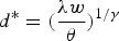 $d^{\ast} =\lpar \displaystyle{{\lambda w}\over{\theta}}\rpar ^{1/\gamma}$ this condition becomes
 $w\lpar \displaystyle{{\lambda w}\over{\theta}}\rpar ^{1/\gamma } \lt T \Rightarrow w \lt T^{{{\gamma}\over{1+\gamma}}}\lpar \displaystyle{{\theta }\over{\lambda}}\rpar ^{{{1}\over{1+\gamma}}}$.
Define 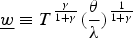 $\underline{w} \equiv T^{{{\gamma}\over{1+\gamma}}}\lpar \displaystyle{{\theta}\over{\lambda}}\rpar ^{{{1}\over{1+\gamma}}}$.
In summary, we can derive the labor supply function to be  $d^\ast = \lpar \displaystyle{{\lambda w}\over{\theta}}\rpar ^{{{1}\over{\gamma}}}$.
Case 2: wd > T
In this case, λ = 1, and the captain's utility becomes:
 $$U\lpar w\comma \; d\rpar = \lpar wd - T\rpar - \displaystyle{{\theta}\over{1+\gamma}}d^{1+\gamma}$$
Solving the FOC for d, we have 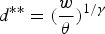 $d^{\ast\ast} = \lpar \displaystyle{{w}\over{\theta}}\rpar ^{1/\gamma}$. This optimal value of d has to satisfy the condition
 $$wd^{\ast\ast} \gt T \Rightarrow w\left(\displaystyle{{w}\over{\theta}}\right)^{1/\gamma} \gt T\Rightarrow w \gt T^{{{\gamma}\over{1+\gamma}}}\theta^{{1}\over{1+\gamma}}. \hbox{ Define }\overline{w}\equiv T^{{\gamma}\over{1+\gamma}}\theta^{{1}\over{1+\gamma}}.$$
In summary, given  $w \gt \overline{w}$ we can derive the labor supply function to be
 $d^{\ast\ast} = \lpar \displaystyle{{w}\over{\theta}}\rpar ^{1/\gamma}$.
Case 3: wd = T
Case 3 also corresponds to the case in which the daily revenue satisfies the condition:  $\underline{w} \lt w \lt \overline{w}$. Put differently, the labor supply is
 $d = \displaystyle{{T}\over{w}}$ given
 $\underline{w} \lt w \lt \overline{w}$.
From cases 1, 2 and 3 we can derive the labor supply function of the captain as follows:
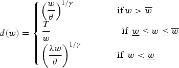 $$d\lpar w\rpar = \left\{\matrix{ \left(\displaystyle{{w}\over{\theta}}\right)^{1/\gamma} \hfill & \hbox{if} \, w \gt \overline{w} \cr \displaystyle{{T}\over{w}} \hfill & \quad \quad \quad \hbox{ if } \, \underline{w} \le w\le \overline{w} \cr \left(\displaystyle{{\lambda w}\over{\theta}}\right)^{1/\gamma} & \hbox{ if } \, w \lt \underline{w}}\right.$$
where 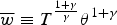 $\overline{w}\equiv T^{{1+\gamma}\over{\gamma}}\theta^{1+\gamma}$ and
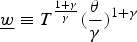 $\underline{w}\equiv T^{{1+\gamma}\over{\gamma}}\lpar \displaystyle{{\theta}\over{\gamma}}\rpar ^{1+\gamma}$.
In addition to the positive relationship between daily revenue and labor supply as predicted by standard models of labor supply, we can see that this relationship is negative when  $w\in\lpar \underline{w}\comma \; \overline{w}\rpar $. Thus, the revenue target model can address a broader range of impacts that daily revenue may have on the fishing trip length. Under the revenue target model, it is plausible that an increase in daily fishing revenue results in shorter trips. The following section empirically explores how closely the revenue target model describes the behavior of Hawaii's longline fishermen.
4. Characteristics of the Hawaii-based longline fishery
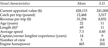
The longline fishery in Hawaii can be characterized as a multi-species targeted fishery. The industry was first introduced by Japanese immigrants in the early 1900s. For a relatively long time the fleet had included a small number of vessels with simple technology. Significant change happened in the late 1980s when a large number of high capital intensive vessels from the U.S. mainland entered Hawaii's longline fishery. The number of active vessels has also been on the rise. There are 135 active longline vessels at present. Table 1 presents basic characteristics of vessels surveyed in the 2004 Hawaii-based longline technology survey. As can be seen from table 1, Hawaii's longline vessels vary greatly in most of the basic characteristics. Some vessels are very large and capital intensive, while others are small and more labor intensive. Some vessels were built around the 1940s while others were built just a few years ago. Variations in vessels’ characteristics may result in a large standard deviation (S.D.) in catch per trip and trip's revenue.
Basic characteristics of Hawaii's longline vessels

Notes: aData is provided by the Coast Guard.
5. Empirical evidence
5.1. Data source and model specifications
Information on the number of fishing days by trip and trip revenue is obtained from 2004 logbook data and 2004 auction data, respectively. It is worth noting that the swordfish fishery was closed in Hawaii from 2002 to 2004 and was re-opened in 2004 under a ‘set cap’ program. Given this special feature of Hawaii's swordfish fishery, our data includes information on the tuna fishery only. Hereafter, longline fishery refers to only the tuna fishery. The logbook is compiled by the National Oceanic and Atmospheric Administration (NOAA). The auction data is collected by the Hawaii Division of Aquatic Resources (HDAR). The logbook data contains information on the number of fishing days for every longline trip in 2004, and the auction data records the trip revenue for each longline vessel in that same year. These two data sets were combined for the estimation of the empirical model.
It is worth noting that there are a number of limitations in the data that make it difficult to parse the underlying reason for the observed data patterns, i.e., a lack of information on dockside prices or contractual shares. Thus, we are cautious when drawing inferences from the associated results.
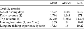
Table 2 presents the summary statistics of the main variables. The average length of a fishing trip in Hawaii's longline fishery is about 19 days. Variation in the number of fishing days is relatively large. An average vessel earns about $32,000 per trip or $1,800 per fishing day.
Summary statistics

The S.D. in fish revenues are relatively large, reflecting the diversity of vessel characteristics within the fisheries. About 50 per cent of captains have spent 16 years in longline fishing. In terms of the vessels’ capacity, about 35 per cent of vessels have an icemaker.
5.2. Model specifications
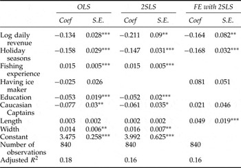
Given that the number of fishing days is count data, one can use a generalized linear model such as a Poisson model to investigate the relationship between the number of fishing days and daily revenue. In this study, we are more interested in the elasticity of fishing days with respect to daily revenue; thus we take the log of fishing days, in turn making the dependent variable continuous. We then use a standard linear model accordingly. Our approach is the same as the one used in the studies of taxi drivers (e.g., Camerer et al., Reference Camerer, Babcock, Loewenstein and Thaler1997; Chou, Reference Chou2002). To check the robustness of the results, we also run the Poisson model. As can be seen from table 3a, the finding indicates a more significant negative relationship between number of fishing days and daily revenue than other model specifications.
Estimated daily fishing revenue elasticity from OLS, 2SLS and fixed effect with instrumental variable models

Notes: ***p < 0.01; **p < 0.05; *p < 0.1.
We conducted robust regression and adjusted S.E. for correlations within individuals.
We start with the basic empirical model, which takes the following form:
 $$\ln D_{it} =\eta \ln w_{it} + X_{it} \beta + \varepsilon_{it}$$
where D u represents the number of fishing days by vessel i on trip t, w it is the average daily revenue of vessel i on trip t, X it are the vessel's characteristics that may impact the trip's fishing length; and ɛit is the standard random error term. Camerer et al. (Reference Camerer, Babcock, Loewenstein and Thaler1997) point out that this method of estimating w it is very similar to that used in the labor supply literature, where wage rate is estimated by dividing yearly (monthly) income by yearly (monthly) working hours. Thus, η is interpreted as the daily revenue elasticity.
We include a binary variable indicating the presence of an icemaker as well as the vessel's length to proxy for the vessel's capacity to stay longer in the ocean; hereafter we term it ‘staying power’. To account for the high demand for fish during the holiday season, we use a binary variable to represent the holiday seasons of Thanksgiving, Christmas and New Year.
In terms of model specification, ideally one should look at the daily revenue in a given trip. This makes it possible to estimate the accumulated revenue on any given fishing day. The cumulative revenue is the deciding factor influencing whether the captain continues to fish or not. However, we do not have information on daily revenue for each individual fishing trip; thus we use the average daily revenue instead as the independent variable.
The use of the average daily revenue may cause potential measurement error. Camerer et al. (Reference Camerer, Babcock, Loewenstein and Thaler1997) and Chou (Reference Chou2002), in their studies on taxi drivers, mention that there may have been measurement errors in the recorded number of driving hours. This problem is known as division bias in labor economics studies (Borjas, Reference Borjas1980). Likewise, one may suspect potential measurement errors in the number of fishing days compiled in the logbook. If such is the case, inflated records may increase the number of fishing days and deflate average trip revenue, while deflated records may decrease the number of fishing days and inflate average trip revenue. Both cases of misreporting fishing days lead to spurious negative elasticity. On the other hand, the daily revenue elasticity may be biased towards zero due to an overreporting of total trip revenue. These two sources of bias will either reinforce or counteract each other, depending on whether the true daily revenue elasticity is positive or negative. Therefore, the net effect is uncertain.
In the fisheries context, the logbook contains the record of the number of fishing days made by each vessel, as it is required by law for fishermen to complete their logs. After every trip, NOAA collects the logbook directly from the captain and ensures that key information, such as fishing days, is recorded correctly. Thus, the data quality, particularly regarding fishing trip days, is quite accurate. Potential measurement errors are more likely to come from the trip revenue data.
Greene (Reference Greene2004) points out that measurement error in the dependent variable is less serious than in the independent variable. Accordingly, we will mainly focus on correcting potential measurement errors in the independent variable (i.e., the daily revenue). The corrections are made by finding an appropriate instrumental variable. Given the data available, we use the average daily fish revenue of other vessels landing on the same day as the instrument for daily revenue. In theory, a good instrument has the covariance of zero, or is unrelated to total fishing days, and has a strong correlation with the daily revenue of the concerned vessel. We believe that the chosen variable has minimal or no impact on the captain's decision to adjust the trip length (dependent variable) and is not highly correlated with the error terms in the trip length equation. We have also found that the greater (lower) the daily revenue of other vessels, the higher (lower) the daily revenue of the concerned vessel, since they face the same market conditions at the auction. Understandably, this interpretation is made under the assumption that there is not much variation in the fishing conditions.
Another practical consideration is whether the chosen instrument is strong. Cameron and Trivedi (Reference Cameron and Trivedi2006) point out that the weak instrumental variable (IV) estimator may be markedly biased in finite samples even though it is asymptotically consistent. To check whether or not the IV is weak, we use the Cragg–Donald Wald statistics, which is an F-statistic in the first stage of the two-stage least squares (2SLS) model, and compare it with the Stock and Yogo (Reference Stock, Yogo, Andrews and Stock2005) critical values to check whether the IV is weak or not. The Cragg–Donald Wald statistics of 21.75 from our 2SLS model indicate a reasonably strong IV.
We realize that the above chosen IV is not perfect in any way. That being said, we believe that it is the best IV we can have given the data at hand. Also, we present both models with and without the IVs in all analyses to check whether the findings are consistent.
As a final comment in this section, note that our data has the underlying panel structure. Following Stock and Watson (Reference Stock and Watson2006), we cluster S.E.s at the vessel level to have S.E.s that are robust to both heteroskedasticity and intra-group correlation.
5.3. Main empirical results
Table 3a presents the results of the estimation from OLS, 2SLS and fixed effect with IV models. The key finding is that daily fishing revenue has a negative and significant impact on the number of fishing days in all models. That is, the higher the daily revenue is, the shorter the fishing trip. This finding is consistent with the studies of taxi drivers by Camerer et al. (Reference Camerer, Babcock, Loewenstein and Thaler1997) and Chou (Reference Chou2002). From the insights of Heath et al. (Reference Heath, Larrick and Wu1999), we can infer that fishermen seem more motivated to reach the revenue target than to surpass it.
We also find that the absolute value of the estimated revenue elasticity for the 2SLS model is marginally greater than the OLS. This result implies that there may be marginal measurement error in the IV (Cameron and Trivedi, Reference Cameron and Trivedi2006). In comparison with the Camerer et al. (Reference Camerer, Babcock, Loewenstein and Thaler1997) and Chou (Reference Chou2002) studies, the elasticity of labor supply with respect to daily revenue in the fisheries is smaller in magnitude. The smaller elasticity may reflect that fishermen have less flexibility in choosing the length of a fishing trip due to the vessel capacity constraints.
In addition to daily revenue, other variables also have significant and expected effects on the number of fishing days. Bigger vessels, as indicated by having greater length, are capable of longer fishing trips. From the estimations, we can also infer that trip length is significantly shorter during the holiday seasons. One possible reason is that fishermen receive higher profits due to higher prices from the increased demand for fish during the holidays. Accordingly, there is an incentive to shorten the fishing trip, in exchange for increasing the number of fishing trips.
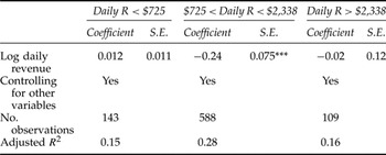
Before moving on to the next section, it is worth noting that, from equation (4) in the model, one would expect the captain to behave differently depending on the daily revenue level.Footnote 4 To verify this prediction empirically, one way is to run the model separately for different samples of vessels by their daily revenues. Table 3b shows that the majority of fishing trips (588 out of 840) indicate a negative correlation between fishing length and daily revenue. Smaller samples of trips show a positive correlation; however, the findings are not significant. Overall, the results seem consistent with the model's prediction and with those presented in table 3a for the sample as a whole.
Estimated daily fishing revenue elasticity from OLS by range of daily revenue

Notes: ***p < 0.01.
We conducted robust regression and adjusted S.E. for correlations within individuals.
$725 and $2,338 correspond to the 25th and 75th percentiles of the daily revenue distribution, respectively.
6. Capacity constraints and the revenue target model
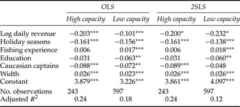
Vessel captains face capacity constraints that prevent them from fishing past a certain amount of time, such as fuel and the preservation of fish quality. Therefore, the prediction of a positive revenue elasticity by the standard model of labor supply may not apply to fishing vessels because their capacity constraints are lower. For instance, the captain might decide to return to the dock even on a good trip to preserve the fish's freshness. To proxy for the dependence of vessels on capacity constraint, we use a ‘staying capacity’ binary variable to indicate whether the vessel has an icemaker and has a median or greater length.Footnote 5 Because of their lesser dependence on capacity constraints, high capacity vessels are more likely to behave according to the standard model of labor supply provided the standard model correctly describes Hawaii's longline captains’ fishing behavior.
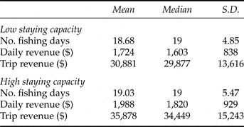
Table 4 summarizes statistics of vessels by staying capacity. As expected, vessels with high staying capacity fish longer than low-capacity vessels, though the difference is insignificant. High staying capacity vessels are also more profitable on a per-trip and per-day basis.
Summary statistics of vessels by staying capacity

To investigate the effect of capacity constraints on fishing behavior under the target revenue framework, we run the regression models by the vessels’ staying capacity (table 5). The results suggest that both groups of vessels with high and low staying capacity seem to behave in accordance with the target revenue model. Also, the difference in daily revenue elasticity among these two groups of vessels is not statistically significant using the Wu–Hausman test (Davidson and MacKinnon, Reference Davidson and MacKinnon1993). Put differently, Hawaii's longline captains follow the same fishing behavior independent of the vessel's ‘staying capacity’.
Estimated daily fishing revenue elasticity by vessel's ‘staying capacity’ using OLS and 2SLS models

Notes: ***p < 0.01; **p < 0.05; *p < 0.1.
We conducted robust regression and adjusted S.E. for correlations within individuals.
7. Conclusions
In this paper we attempt to provide another perspective within the existing labor supply literature. We developed a simple target revenue model to show, under certain conditions, that increases in daily fishing revenue lead to decreases in trip length. Using different model specifications, we found a significantly negative correlation between daily revenue and trip length. The more productive their fishing trip is, the shorter the captains will choose to make their fishing trip. This finding implies that Hawaii's fishermen tend to have a revenue target for their fishing trips. Our study, like those of Camerer et al. (Reference Camerer, Babcock, Loewenstein and Thaler1997), Chou (Reference Chou2002) and Fehr and Goette (Reference Fehr and Goette2007), highlights the relevance of integrating prospect theory into the framework of labor economics.
We also investigated how unique features of the fisheries impact fishermen's behavior under the target revenue framework. We separated the vessels into groups by their staying capacity. We found that Hawaii's longline captains follow the same fishing behavior independent of vessel's ‘staying capacity’.
An interesting finding is that the revenue target model seems to fit the data better. This is consistent with other studies showing that prospect theory is a better description of individual preference than expected utility. Given that fishermen have the flexibility of choosing working duration, having a target of revenue plays a key role in deciding the fishing trip length. By incorporating the target revenue, the prospect theory gives a better description of decision-making behavior in fisheries and occupations that share a similar nature of work duration flexibility such as taxi driving.
This paper can be improved in a number of respects. The use of an imperfect IV may lead to less biased estimations at the expense of an efficiency loss. In some estimations, the results from the 2SLS model became less significant than the OLS due to increase in the S.E.s. An approach based on a system of structural equations and natural experiments may help to solve this problem (Cameron and Trivedi, Reference Cameron and Trivedi2006).
As a potential extension of the paper, we can conduct further field experiments with Hawaii's longline fishermen to measure the loss aversion parameter for each participant and identify a model that best describes the fishermen's risk behavior. Fehr and Goette (Reference Fehr and Goette2007) suggest either a reference dependence model or a neoclassical model with non-separable preferences. They also find that loss-averse participants are more likely to behave in accordance with the target model. Integrating the risk behavior of fishermen under prospect theory, of which loss aversion is an important aspect, into the framework of fisheries decision making is a promising area in fisheries research.
Another potential extension of this study is to investigate how well the revenue target model performs relative to the hazard model by Farber. In his study of taxi cab drivers, Farber (Reference Farber2005, Reference Farber2008) finds the standard model more favorable than the target revenue model. Our study of Hawaii's longline fisheries reveals that the target revenue model gives robust findings under different model specifications. Accordingly, we believe that our results will probably hold under Farber's approach. That being said, the current study would be more complete if we could also use Farber's approach to check the robustness of the results. However, we presently do not have information on the daily vessel revenue for a given fishing trip. Improvement in logbook data collection will allow us to investigate the relative performance of the target revenue model against the standard model of labor supply.
Finally, like Farber (Reference Farber2005, Reference Farber2008) and Crawford and Meng (Reference Crawford and Meng2011), we take targets as givens rather than modeling them as endogenously determined. Further analysis on how these targets are formed and adjusted over time is a promising direction for future research.