1 Introduction
For flows whose unsteadiness proceeds from an intrinsic instability mechanism, linear and weakly nonlinear stability analyses provide a rigorous mathematical foundation to explain the initial growth of disturbances of a certain scale and frequency, and the leading-order nonlinear effects associated with small-amplitude disturbances. The quality of the prediction, however, deteriorates rapidly with increasing distance from the instability threshold, as the perturbative nature of these approaches imposes the condition to build the fluctuation as successive-order corrections to the leading eigenmode of the base flow (i.e. the steady state sustaining the instability), whose spatial structure can differ considerably from that of the nonlinearly saturated oscillation (Dušek, Le Gal & Fraunié Reference Dušek, Le Gal and Fraunié1994; Noack et al.
Reference Noack, Afanasiev, Morzynski, Tadmor and Thiele2003). As an illustration, the vortex street of shed vortices that form the wake of a circular cylinder sets in at Reynolds number
 $Re=47$
, but the inaccuracy in the frequency computed by linear stability analysis is already
 $30\,\%$
at values of
 $Re$
as low as
 $80$
(Barkley Reference Barkley2006), while that on the weakly nonlinear oscillation amplitude exceeds
 $100\,\%$
(Mantič-Lugo, Arratia & Gallaire Reference Mantič-Lugo, Arratia and Gallaire2014).
It is the time-averaged mean flow, not the base flow, that is key in understanding the growth of disturbances while encompassing the nonlinearity of the system (Maurel, Pagneux & Wesfreid Reference Maurel, Pagneux and Wesfreid1995; Zielinska et al. Reference Zielinska, Goujon-Durand, Dušek and Wesfreid1997; Noack et al. Reference Noack, Afanasiev, Morzynski, Tadmor and Thiele2003). A simplified model for the saturation of the cylinder flow has been proposed recently by Mantič-Lugo et al. (Reference Mantič-Lugo, Arratia and Gallaire2014) using a so-called self-consistent approach coupling the mean flow and its leading eigenmode via formation of Reynolds stresses. The authors show that saturation occurs when the eigenmode has zero linear growth rate, wherein the model predicts accurately the mean flow, Reynolds stresses, frequency, amplitude and structure of the fluctuation obtained by direct numerical simulation (DNS). The model is also relevant to describe the transient development of the instability (Mantič-Lugo, Arratia & Gallaire Reference Mantič-Lugo, Arratia and Gallaire2015), which formalizes the intuitive picture invoked to describe the growth and saturation of disturbances, dating back to Malkus (Reference Malkus1956) and Stuart (Reference Stuart1971): perturbations feed on the unstable base flow and grow first according to the linear theory. When they reach a size large enough for nonlinearities to set in, they feed back via their Reynolds stresses, and distort the base flow into an increasingly stable mean flow, up to the point where the mean flow is linearly marginally stable and perturbations stop growing and saturate. It also rationalizes the fact that the mean flow eigenfrequency agrees well with the exact oscillation frequency, as noticed early in cylinder flows and related bluff-body wakes (Hammond & Redekopp Reference Hammond and Redekopp1997; Pier Reference Pier2002; Barkley Reference Barkley2006).
The above scenario anticipates a linearly marginally stable mean flow because it reduces the consequences of the nonlinearity to mean flow distortions, and neglects another important mechanism that may alter the predictions of the linear theory: the generation of harmonics. The model of Mantič-Lugo et al. (Reference Mantič-Lugo, Arratia and Gallaire2014) relies on the same simplifying assumption. It is thus relevant to the cylinder case, whose mean flow is linearly marginally stable (Barkley Reference Barkley2006) only because vortex shedding is almost monochromatic (Dušek et al. Reference Dušek, Le Gal and Fraunié1994). For flows whose nonlinearity unveils strong higher harmonics, e.g. open cavity flows (Sipp & Lebedev Reference Sipp and Lebedev2007), turbulent wakes (Meliga, Sipp & Chomaz Reference Meliga, Sipp and Chomaz2009b ; Meliga, Pujals & Serre Reference Meliga, Pujals and Serre2012; Meliga, Cadot & Serre Reference Meliga, Cadot and Serre2016b ), or certain regimes of thermosolutal convection flows (Turton, Tuckerman & Barkley Reference Turton, Tuckerman and Barkley2015), the mean flow is generally strongly linearly unstable and a simplified formulation capable of similarly accurately unravelling the mechanics of saturation is lacking. This research intends to fill in the gap using augmented self-consistent models coupling the mean flow to multiple harmonic linear disturbances interacting nonlinearly with one another and feeding back on the mean flow via formation of Reynolds stresses. Such an approach is applied to the flow over a square cavity, for which we show that only the second harmonic needs to be retained.
The paper is organized as follows. The configuration is described in § 2, and the unsteady cavity flow is characterized in § 3 using DNS and classical linear stability analysis. The second-order self-consistent model is derived in § 4, and its ability to describe the mechanics of saturation is assessed in § 5 from exhaustive comparison to time and phase averages of DNS data. Connection with weakly nonlinear analysis is addressed in § 6, where we also evidence the ability of the method to encompass the effect of higher-order harmonics, and discuss how to anticipate an appropriate truncation order.
2 Flow configuration
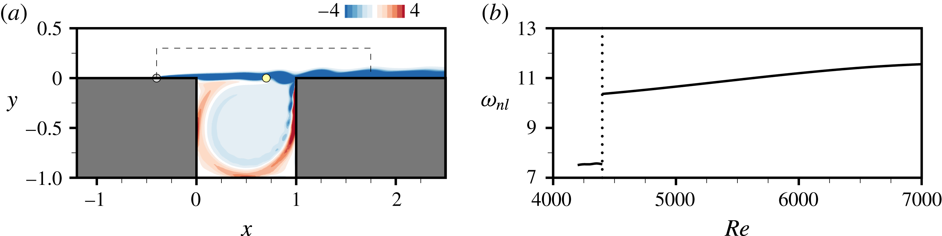
We consider the two-dimensional incompressible flow over the open square cavity described in detail by Sipp & Lebedev (Reference Sipp and Lebedev2007). Suffice it to say here that a uniform velocity field is imposed at the inlet boundary and that a laminar boundary layer starts to develop between the inlet and the upstream edge of the cavity, the exact position being adjustable via an appropriate choice of boundary conditions; see figure 1(a). The free-stream velocity and cavity width (or height) are used to make all quantities non-dimensional. We denote by
 $\boldsymbol{u}=(u,v)$
the velocity field of components
 $u$
and
 $v$
in the streamwise
 $x$
and cross-stream
 $y$
directions and by
 $p$
the pressure. The flow is governed by the Navier–Stokes equations (NSE) written in compact form as
 $$\begin{eqnarray}\unicode[STIX]{x2202}_{t}\boldsymbol{u}+\boldsymbol{N}(\boldsymbol{u})=\mathbf{0},\end{eqnarray}$$
where
 $$\begin{eqnarray}\boldsymbol{N}(\boldsymbol{u})=\boldsymbol{u}\boldsymbol{\cdot }\unicode[STIX]{x1D735}\boldsymbol{u}+\unicode[STIX]{x1D735}p-Re^{-1}\unicode[STIX]{x1D6FB}^{2}\boldsymbol{u}\end{eqnarray}$$
is the Navier–Stokes operator, whose dependence on
 $p$
is omitted to ease the notation. Because of incompressibility, it is understood that all velocity fields are divergence-free; therefore we will not write this condition explicitly.
All calculations are performed on the same computational domain made of
 $194\,447$
triangles, equipped with the
 $L^{2}$
inner product
 $(\cdot |\cdot )$
and related norm
 $\Vert \cdot \Vert$
. We perform DNS of (2.1) with the finite-element solver presented in Meliga et al. (Reference Meliga, Boujo, Pujals and Gallaire2014). Time integration is achieved using a second-order-accurate Crank–Nicolson scheme with time step
 $\unicode[STIX]{x0394}t=10^{-2}$
. Unless specified otherwise, all time-averaged quantities (as denoted by
 $\overline{\,\cdot \,}\,$
) are obtained by averaging on-the-fly over
 $200$
time units after the flow has settled down to a periodic regime, which represents
 ${\sim}300$
cycles depending on the Reynolds number. We also use the Newton method to compute the base cavity flow
 $\boldsymbol{u}_{b}$
, i.e. the solution to the steady NSE
 $$\begin{eqnarray}\boldsymbol{N}(\boldsymbol{u}_{b})=\mathbf{0},\end{eqnarray}$$
whose stability is analysed using the Arnoldi method. In the following, we denote by
 $\hat{\boldsymbol{u}}_{10b}$
the leading eigenmode of linear growth rate
 $\unicode[STIX]{x1D70E}_{0b}$
and eigenfrequency
 $\unicode[STIX]{x1D714}_{0b}$
; hence, the solution to the eigenvalue problem
 $$\begin{eqnarray}(\unicode[STIX]{x1D70E}_{0b}^{}+\text{i}\unicode[STIX]{x1D714}_{0b}^{})\hat{\boldsymbol{u}}_{10b}+\boldsymbol{L}(\boldsymbol{u}_{b})\hat{\boldsymbol{u}}_{10b}=\mathbf{0},\end{eqnarray}$$
where
 $$\begin{eqnarray}\boldsymbol{L}(\boldsymbol{u}_{b})\hat{\boldsymbol{u}}=\boldsymbol{u}_{b}\boldsymbol{\cdot }\unicode[STIX]{x1D735}\hat{\boldsymbol{u}}+\hat{\boldsymbol{u}}\boldsymbol{\cdot }\unicode[STIX]{x1D735}\boldsymbol{u}_{b}+\unicode[STIX]{x1D735}\hat{p}-Re^{-1}\unicode[STIX]{x1D6FB}^{2}\hat{\boldsymbol{u}},\end{eqnarray}$$
is the linearized Navier–Stokes (LNS) operator. We also determine the linear stability of the time-averaged mean flow
 $\overline{\boldsymbol{u}}$
, whose leading eigenmode
 $\hat{\boldsymbol{u}}_{10m}$
of linear growth rate
 $\unicode[STIX]{x1D70E}_{0m}$
and eigenfrequency
 $\unicode[STIX]{x1D714}_{0m}$
is the solution to the eigenvalue problem
 $$\begin{eqnarray}(\unicode[STIX]{x1D70E}_{0m}+\text{i}\unicode[STIX]{x1D714}_{0m})\hat{\boldsymbol{u}}_{10m}+\boldsymbol{L}(\overline{\boldsymbol{u}})\hat{\boldsymbol{u}}_{10m}=\mathbf{0}.\end{eqnarray}$$
3 Direct numerical simulations and eigenmode analysis
Figure 1(a) shows a snapshot of vorticity at
 $Re=6000$
. The shear layer rolls up into large-scale vortices that ultimately impact the downstream edge of the cavity. A pressure wave forms, travels upstream via the recirculating flow in the cavity, and excites the shear layer at the upstream edge. This causes new perturbations to grow again into large-scale vortices via Kelvin–Helmholtz instability. This feedback loop leads to a linear global instability, and the flow settles on a periodic limit cycle (Åkervik et al.
Reference Åkervik, Ehrenstein, Gallaire and Henningson2008; Barbagallo, Sipp & Schmid Reference Barbagallo, Sipp and Schmid2009). The curve of the oscillation frequency against
 $Re$
shown in figure 1(b) presents a discontinuity at
 $Re=4400$
, which is because the base flow undergoes successive Hopf bifurcations at
 $Re_{c1}=4114$
(in good agreement with the threshold value
 $4140$
reported by Sipp & Lebedev Reference Sipp and Lebedev2007) and
 $Re_{c2}=4348$
. Both eigenmodes exchange dominance at
 $Re=4567$
, after which the mode selection follows the ‘largest growth rate’ criterion. This bifurcation sequence is robust in the sense that, while small changes in the set-up (especially the position at which the boundary layer starts to develop) yield small variations in the instability thresholds, the flow oscillations systematically end up being driven by the second eigenmode at sufficiently high Reynolds numbers (not shown here). The focus in the sequel is thus on the range
 $Re\geqslant 4400$
, with default value set to
 $Re=6000$
.
(a) Isocontours of vorticity showing the periodic ejection of vortices from the upstream edge of the cavity,
 $Re=6000$
. The streamwise velocity spectrum in figure 3 is measured at the position
 $(x,y)=(0.7,0)$
of the grey symbol, and the boundary layer develops from the position
 $(x,y)=(-0.4,0)$
of the yellow symbol. The dashed line delimits the inner domain
 $(x,y)\in [-0.4,1.75]\times [-1,0.3]$
. (b) Oscillation frequency
 $\unicode[STIX]{x1D714}_{nl}^{}$
against
 $Re$
.

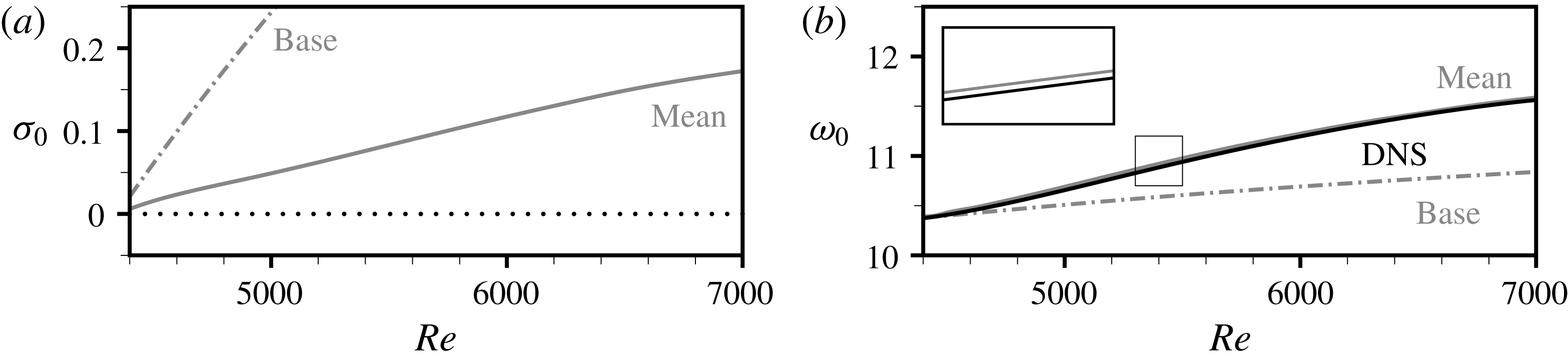
The mean cavity flow fails to comply with the linear marginal stability criterion of Mantič-Lugo et al. (Reference Mantič-Lugo, Arratia and Gallaire2014), as evidenced by the large positive growth rate
 $\unicode[STIX]{x1D70E}_{0m}=0.117$
of the leading eigenmode at
 $Re=6000$
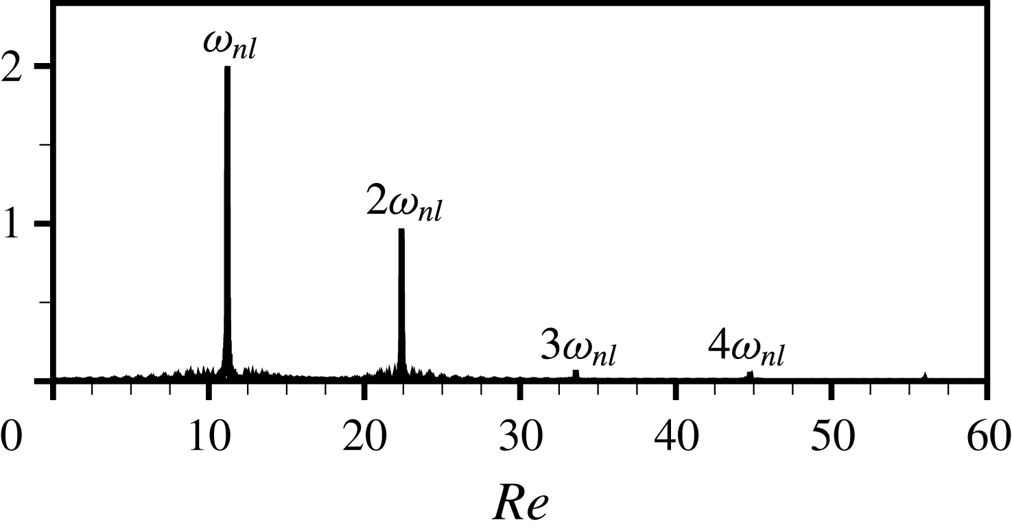
. Figure 2(a) unveils a similar behaviour regardless of the Reynolds number, which is because the nonlinearity generates strong higher harmonics, as evidenced in figure 3 by the spectrum of the streamwise velocity measured in the shear layer at
 $(x,y)=(0.7,0)$
, almost midway between the two edges of the cavity: beyond the peak at the fundamental frequency
 $\unicode[STIX]{x1D714}_{nl}^{}=11.19$
, we notice a substantial second harmonic at
 $2\unicode[STIX]{x1D714}_{nl}^{}$
, and even third and fourth harmonics (although the peaks at
 $3\unicode[STIX]{x1D714}_{nl}^{}$
and
 $4\unicode[STIX]{x1D714}_{nl}^{}$
are of much smaller magnitudes). Interestingly, the eigenfrequency of the mean flow
 $\unicode[STIX]{x1D714}_{0m}=11.22$
does predict well the nonlinear oscillation frequency (unlike that,
 $\unicode[STIX]{x1D714}_{0b}=10.69$
, of the base flow; see also figure 2(b)), which is a little surprising because, according to Sipp & Lebedev (Reference Sipp and Lebedev2007), the mean flow eigenfrequency is expected to miss the exact frequency in the presence of strong higher harmonics. Such an interpretation, however, issues from an asymptotic analysis valid only close to the instability threshold, while linearly unstable mean flows whose eigenfrequency somehow manages to do well in predicting the frequency have been documented in the context of strongly nonlinear turbulent wakes (Meliga et al.
Reference Meliga, Sipp and Chomaz2009b
, Reference Meliga, Pujals and Serre2012, Reference Meliga, Cadot and Serre2016b
). It is part of the objectives of this research to show that the nonlinearity induced by the higher-order harmonics can help straighten out this apparent contradiction.
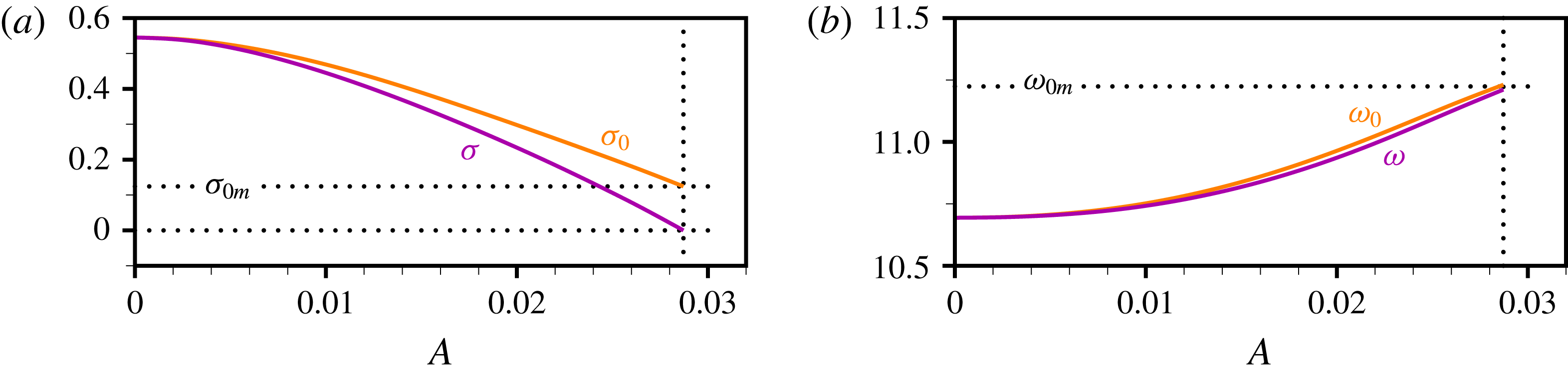
(a) Linear growth rate against
 $Re$
. The value
 $\unicode[STIX]{x1D70E}_{0m}$
(respectively
 $\unicode[STIX]{x1D70E}_{0b}$
) obtained by linear stability analysis of the time-averaged mean flow (respectively of the base flow) is shown by the grey line (respectively the dash-dotted grey line). (b) Same as (a) for the eigenfrequency
 $\unicode[STIX]{x1D714}_{0}$
. The nonlinear frequency
 $\unicode[STIX]{x1D714}_{nl}^{}$
extracted from the DNS is shown by the black line.

4 Self-consistent model
4.1 Theoretical formalism
The self-consistent theory is meant to describe the development and saturation of the instability based on a parametrized approximation of the mean flow–fluctuation interaction. Consider the general situation of a DNS whose initial condition consists of the base flow
 $\boldsymbol{u}_{b}$
plus its unit-norm leading eigenmode
 $\hat{\boldsymbol{u}}_{10b}$
with (real) amplitude
 $A_{0}$
but arbitrary phase
 $\unicode[STIX]{x1D719}_{0}$
, i.e.
 $$\begin{eqnarray}\boldsymbol{u}(t=0,\unicode[STIX]{x1D719}_{0})=\boldsymbol{u}_{b}+A_{0}(\hat{\boldsymbol{u}}_{10b}\text{e}^{\text{i}\unicode[STIX]{x1D719}_{0}}+\text{c.c.}).\end{eqnarray}$$
Following Mantič-Lugo et al. (Reference Mantič-Lugo, Arratia and Gallaire2015), we study here the evolution of a time-dependent mean flow constructed by averaging at each time instant over the phase of the initial disturbance, i.e.
 $$\begin{eqnarray}\langle \boldsymbol{u}\rangle (t)=\frac{1}{2\unicode[STIX]{x03C0}}\int _{0}^{2\unicode[STIX]{x03C0}}\boldsymbol{u}(t)\,\text{d}\unicode[STIX]{x1D719}_{0}.\end{eqnarray}$$
As a first step, we substitute
 $\langle \boldsymbol{u}\rangle +\boldsymbol{u}^{\prime }$
for
 $\boldsymbol{u}$
in the NSE, where
 $\boldsymbol{u}^{\prime }$
is the zero-mean (in the sense of phase average) fluctuation, to give
 $$\begin{eqnarray}\displaystyle & \displaystyle \unicode[STIX]{x2202}_{t}\langle \boldsymbol{u}\rangle +\boldsymbol{N}(\langle \boldsymbol{u}\rangle )=-\langle \unicode[STIX]{x1D73B}(\boldsymbol{u}^{\prime })\rangle , & \displaystyle\end{eqnarray}$$
 $$\begin{eqnarray}\displaystyle & \displaystyle \unicode[STIX]{x2202}_{t}\boldsymbol{u}^{\prime }+\boldsymbol{L}(\langle \boldsymbol{u}\rangle )\boldsymbol{u}^{\prime }=-\unicode[STIX]{x1D73B}(\boldsymbol{u}^{\prime })+\langle \unicode[STIX]{x1D73B}(\boldsymbol{u}^{\prime })\rangle , & \displaystyle\end{eqnarray}$$
 $\unicode[STIX]{x1D73B}(\boldsymbol{u})=\boldsymbol{u}\boldsymbol{\cdot }\unicode[STIX]{x1D735}\boldsymbol{u}$
the nonlinear advection operator. The second step is to approximate the fluctuation by a Fourier series expansion. We elaborate further on this matter in § 6.2, but we settle here for a second-order expansion, as we anticipate from figure 3 that the effect of the higher-order harmonics will be of a much smaller magnitude. This yields
 $$\begin{eqnarray}\boldsymbol{u}^{\prime }(t)=A(t)\boldsymbol{u}_{1}(t)\text{e}^{\text{i}\unicode[STIX]{x1D714}t}+A^{2}(t)\boldsymbol{u}_{2}(t)\text{e}^{2\text{i}\unicode[STIX]{x1D714}t}+\text{c.c.},\end{eqnarray}$$
where
 $\unicode[STIX]{x1D714}$
is the fundamental oscillation frequency,
 $\boldsymbol{u}_{1}$
is the structure of the first harmonic, parametrized by its (real) amplitude
 $A$
,
 $\boldsymbol{u}_{2}$
is the structure of the second harmonic, coming (with no loss of generality) with amplitude
 $A^{2}$
, and we allow both the amplitude and the structure of the harmonics to vary in time to reflect the distortions of the fluctuation throughout the development of the instability.
Spectrum of the streamwise shear-layer velocity at
 $(x,y)=(0.7,0)$
for
 $Re=6000$
. All results are normalized for the second harmonic to peak at unity.

As explained in Mantič-Lugo et al. (Reference Mantič-Lugo, Arratia and Gallaire2015), the premise of the self-consistent theory is that there exists a separation of scales between the fast time scale on which the flow oscillates, and the slow time scale on which the oscillations grow in amplitude (similar to the assumption made in weakly nonlinear analysis to compute the amplitude of the unstable eigenmode from an amplitude equation). For the cavity flow, the relevance of this assumption is supported by the results documented in § 5.2; therefore we invoke a quasi-static approximation to slave the (phase-averaged) mean flow
 $\langle \boldsymbol{u}\rangle$
and the harmonics
 $\boldsymbol{u}_{1}$
and
 $\boldsymbol{u}_{2}$
to their forcing by the self-interaction of the fluctuation, as described by the right-hand sides (RHS) of system (4.3). In practice, this amounts to assuming at each time instant a steady mean flow and purely oscillating harmonics, for which averaging over the phase is equivalent to averaging in time over a period. Substituting in (4.3) and neglecting all higher interactions yields
 $$\begin{eqnarray}\displaystyle & \displaystyle \boldsymbol{N}(\langle \boldsymbol{u}\rangle )=-A^{2}\unicode[STIX]{x1D74D}(\boldsymbol{u}_{1})-A^{4}\unicode[STIX]{x1D74D}(\boldsymbol{u}_{2}), & \displaystyle\end{eqnarray}$$
 $$\begin{eqnarray}\displaystyle & \displaystyle (\unicode[STIX]{x1D70E}+\text{i}\unicode[STIX]{x1D714})\boldsymbol{u}_{1}+\boldsymbol{L}(\langle \boldsymbol{u}\rangle )\boldsymbol{u}_{1}=-A^{2}\unicode[STIX]{x1D753}(\boldsymbol{u}_{1}^{\ast },\boldsymbol{u}_{2}), & \displaystyle\end{eqnarray}$$
 $$\begin{eqnarray}\displaystyle & \displaystyle 2(\unicode[STIX]{x1D70E}+\text{i}\unicode[STIX]{x1D714})\boldsymbol{u}_{2}+\boldsymbol{L}(\langle \boldsymbol{u}\rangle )\boldsymbol{u}_{2}=-\unicode[STIX]{x1D73B}(\boldsymbol{u}_{1}), & \displaystyle\end{eqnarray}$$
 $\unicode[STIX]{x1D753}(\boldsymbol{u},\boldsymbol{v})=\boldsymbol{u}\boldsymbol{\cdot }\unicode[STIX]{x1D735}\boldsymbol{v}+\boldsymbol{v}\boldsymbol{\cdot }\unicode[STIX]{x1D735}\boldsymbol{u}$
is the linearized advection operator,
 $^{\ast }$
indicates complex conjugation, and we note
 $\unicode[STIX]{x1D74D}(\boldsymbol{u})=\unicode[STIX]{x1D753}(\boldsymbol{u},\boldsymbol{u}^{\ast })$
. In (4.5b
),
 $\unicode[STIX]{x1D70E}$
is the growth rate of the first harmonic (assumed to be relative neither to a particular point in space, nor to a particular component of the solution), and we take the second harmonic to grow at the same rate
 $2\unicode[STIX]{x1D70E}$
as the source term
 $\unicode[STIX]{x1D73B}(\boldsymbol{u}_{1})$
in (4.5c
), hence
 $$\begin{eqnarray}\unicode[STIX]{x2202}_{t}(A\boldsymbol{u}_{1})=\unicode[STIX]{x1D70E}A\boldsymbol{u}_{1}\quad \text{and}\quad \unicode[STIX]{x2202}_{t}(A^{2}\boldsymbol{u}_{2})=2\unicode[STIX]{x1D70E}A^{2}\boldsymbol{u}_{2}.\end{eqnarray}$$
Equation (4.5a
) now defines the mean flow as a solution to the steady NSE forced by the Reynolds stresses of the fluctuation, while (4.5b
) and (4.5c
) conversely define the harmonics as forced solutions to the NSE linearized about the mean flow, with the RHS of (4.5b
) (respectively the RHS of (4.5c
)) accounting for the self-interaction of the fluctuation at frequency
 $\unicode[STIX]{x1D714}$
, that feeds back on the first harmonic (respectively the self-interaction at frequency
 $2\unicode[STIX]{x1D714}$
that generates the second harmonic).
System (4.5) does provide a self-consistent description of the mean flow–fluctuation interaction, in the sense that all perturbation structures are those whose Reynolds stresses force the mean flow in a manner such that the mean flow generates exactly the aforementioned perturbations. However, it cannot be solved as is, because both
 $\unicode[STIX]{x1D70E}$
and
 $\unicode[STIX]{x1D714}$
are part of the unknowns. Therefore, we further decompose the first harmonic into
 $$\begin{eqnarray}\boldsymbol{u}_{1}=\hat{\boldsymbol{u}}_{10}+\boldsymbol{u}_{1\bot },\end{eqnarray}$$
where
 $\hat{\boldsymbol{u}}_{10}$
is the leading eigenmode of the mean flow, of linear growth rate
 $\unicode[STIX]{x1D70E}_{0}$
and eigenfrequency
 $\unicode[STIX]{x1D714}_{0}$
, hence solution to the eigenvalue problem
 $$\begin{eqnarray}(\unicode[STIX]{x1D70E}_{0}+\text{i}\unicode[STIX]{x1D714}_{0})\hat{\boldsymbol{u}}_{10}+\boldsymbol{L}(\langle \boldsymbol{u}\rangle )\hat{\boldsymbol{u}}_{10}=\mathbf{0},\end{eqnarray}$$
and
 $\boldsymbol{u}_{1\bot }$
is the projection on the hyperplane spanned by the remaining eigenmodes. It is worth insisting that (4.8) reflects by no means the time dependence of the eigenmode. The model takes both
 $\hat{\boldsymbol{u}}_{10}$
and
 $\boldsymbol{u}_{1\bot }$
to have the same growth rate
 $\unicode[STIX]{x1D70E}$
and frequency
 $\unicode[STIX]{x1D714}$
as the first harmonic, as we shall clarify that those precisely differ from the values
 $\unicode[STIX]{x1D70E}_{0}$
and
 $\unicode[STIX]{x1D714}_{0}$
obtained by linear stability analysis on behalf of the resonance between the first harmonic and its nonlinear interaction with the second harmonic. In the following, we term
 $\boldsymbol{u}_{1\bot }$
the orthogonal component of the first harmonic, which is a small misuse of language because, owing to the non-normality of the LNS operator (Chomaz Reference Chomaz2005),
 $\boldsymbol{u}_{1\bot }$
is orthogonal not to the leading eigenmode, but to the adjoint leading eigenmode of the mean flow, i.e. the solution
 $\hat{\boldsymbol{u}}_{10}^{\dagger }$
to the eigenvalue problem
 $$\begin{eqnarray}(\unicode[STIX]{x1D70E}_{0}-\text{i}\unicode[STIX]{x1D714}_{0})\hat{\boldsymbol{u}}_{10}^{\dagger }+\boldsymbol{L}^{\dagger }(\langle \boldsymbol{u}\rangle )\hat{\boldsymbol{u}}_{10}^{\dagger }=\mathbf{0},\end{eqnarray}$$
where
 $$\begin{eqnarray}\boldsymbol{L}^{\dagger }(\langle \boldsymbol{u}\rangle )\hat{\boldsymbol{u}}=-\langle \boldsymbol{u}\rangle \boldsymbol{\cdot }\unicode[STIX]{x1D735}\hat{\boldsymbol{u}}+\hat{\boldsymbol{u}}\boldsymbol{\cdot }\unicode[STIX]{x1D735}\langle \boldsymbol{u}\rangle ^{\text{T}}+\unicode[STIX]{x1D735}\hat{p}-Re^{-1}\unicode[STIX]{x1D6FB}^{2}\hat{\boldsymbol{u}},\end{eqnarray}$$
is the adjoint of the LNS operator. The governing equation for
 $\boldsymbol{u}_{1\bot }$
is obtained by subtracting (4.8) from (4.5b
), hence
 $$\begin{eqnarray}(\unicode[STIX]{x1D70E}_{0}+\text{i}\unicode[STIX]{x1D714}_{0})\boldsymbol{u}_{1\bot }+\boldsymbol{L}(\langle \boldsymbol{u}\rangle )\boldsymbol{u}_{1\bot }=-A^{2}\unicode[STIX]{x1D753}(\boldsymbol{u}_{1}^{\ast },\boldsymbol{u}_{2})-\unicode[STIX]{x1D6FE}\boldsymbol{u}_{1},\end{eqnarray}$$
where the detuning parameter
 $$\begin{eqnarray}\unicode[STIX]{x1D6FE}=\unicode[STIX]{x1D6FE}_{r}+\text{i}\unicode[STIX]{x1D6FE}_{i}=(\unicode[STIX]{x1D70E}-\unicode[STIX]{x1D70E}_{0})+\text{i}(\unicode[STIX]{x1D714}-\unicode[STIX]{x1D714}_{0})=-A^{2}\frac{(\hat{\boldsymbol{u}}_{10}^{\dagger }\mid \unicode[STIX]{x1D753}(\boldsymbol{u}_{1}^{\ast },\boldsymbol{u}_{2}))}{(\hat{\boldsymbol{u}}_{10}^{\dagger }\mid \hat{\boldsymbol{u}}_{10})}\end{eqnarray}$$
is made explicit by taking the inner product of (4.11) with
 $\hat{\boldsymbol{u}}_{10}^{\dagger }$
and integrating by parts.
We can now recast (4.5) into the alternative, closed system
 $$\begin{eqnarray}\displaystyle & \displaystyle \boldsymbol{N}(\langle \boldsymbol{u}\rangle )=-A^{2}\unicode[STIX]{x1D74D}(\hat{\boldsymbol{u}}_{10}+\boldsymbol{u}_{1\bot })-A^{4}\unicode[STIX]{x1D74D}(\boldsymbol{u}_{2}), & \displaystyle\end{eqnarray}$$
 $$\begin{eqnarray}\displaystyle & \displaystyle (\unicode[STIX]{x1D70E}_{0}+\text{i}\unicode[STIX]{x1D714}_{0})\hat{\boldsymbol{u}}_{10}+\boldsymbol{L}(\langle \boldsymbol{u}\rangle )\hat{\boldsymbol{u}}_{10}=\mathbf{0}, & \displaystyle\end{eqnarray}$$
 $$\begin{eqnarray}\displaystyle & \displaystyle (\unicode[STIX]{x1D70E}_{0}-\text{i}\unicode[STIX]{x1D714}_{0})\hat{\boldsymbol{u}}_{10}^{\dagger }+\boldsymbol{L}^{\dagger }(\langle \boldsymbol{u}\rangle )\hat{\boldsymbol{u}}_{10}^{\dagger }=\mathbf{0}, & \displaystyle\end{eqnarray}$$
 $$\begin{eqnarray}\displaystyle & \displaystyle (\unicode[STIX]{x1D70E}_{0}+\text{i}\unicode[STIX]{x1D714}_{0})\boldsymbol{u}_{1\bot }+\boldsymbol{L}(\langle \boldsymbol{u}\rangle )\boldsymbol{u}_{1\bot }=-A^{2}\unicode[STIX]{x1D753}(\hat{\boldsymbol{u}}_{10}^{\ast }+\boldsymbol{u}_{1\bot }^{\ast },\boldsymbol{u}_{2})-\unicode[STIX]{x1D6FE}(\hat{\boldsymbol{u}}_{10}+\boldsymbol{u}_{1\bot }), & \displaystyle\end{eqnarray}$$
 $$\begin{eqnarray}\displaystyle & \displaystyle 2(\unicode[STIX]{x1D70E}_{0}+\text{i}\unicode[STIX]{x1D714}_{0}+\unicode[STIX]{x1D6FE})\boldsymbol{u}_{2}+\boldsymbol{L}(\langle \boldsymbol{u}\rangle )\boldsymbol{u}_{2}=-\unicode[STIX]{x1D73B}(\hat{\boldsymbol{u}}_{10}+\boldsymbol{u}_{1\bot }), & \displaystyle\end{eqnarray}$$
 $$\begin{eqnarray}\displaystyle & \displaystyle \unicode[STIX]{x1D6FE}=-A^{2}\frac{(\hat{\boldsymbol{u}}_{10}^{\dagger }\mid \unicode[STIX]{x1D753}(\hat{\boldsymbol{u}}_{10}^{\ast }+\boldsymbol{u}_{1\bot }^{\ast },\boldsymbol{u}_{2}))}{(\hat{\boldsymbol{u}}_{10}^{\dagger }\mid \hat{\boldsymbol{u}}_{10})}, & \displaystyle\end{eqnarray}$$
 $\langle \boldsymbol{u}\rangle$
,
 $\{\hat{\boldsymbol{u}}_{10},\unicode[STIX]{x1D70E}_{0},\unicode[STIX]{x1D714}_{0}\}$
,
 $\boldsymbol{u}_{1\bot }$
,
 $\boldsymbol{u}_{2}$
,
 $\hat{\boldsymbol{u}}_{10}^{\dagger }$
and
 $\unicode[STIX]{x1D6FE}$
. Those are the equations of our second-order self-consistent model, whose sole free parameter for given Reynolds number is the amplitude
 $A$
of the first harmonic (of course, if
 $\boldsymbol{u}_{2}=\mathbf{0}$
, then
 $\unicode[STIX]{x1D6FE}$
and
 $\boldsymbol{u}_{1\bot }$
are trivially zero and the model consistently reduces to the first-order model of Mantič-Lugo et al. (Reference Mantič-Lugo, Arratia and Gallaire2014)). As further developed in the sequel, solving the model equations for increasing values of the amplitude shapes implicit relationships, e.g.
 $\unicode[STIX]{x1D70E}_{0}=\unicode[STIX]{x1D70E}_{0}(A)$
,
 $\unicode[STIX]{x1D714}_{0}=\unicode[STIX]{x1D714}_{0}(A)$
,
 $\unicode[STIX]{x1D6FE}=\unicode[STIX]{x1D6FE}(A)$
, etc., that link the obtained family of solutions to the development in time of the instability.
4.2 Numerical resolution
System (4.13) can be solved using a simple nested-loop scheme: assuming relevant guesses are at hand for all quantities of interest, an outer loop solves iteratively
 $\langle \boldsymbol{u}\rangle$
to a precision of
 $10^{-12}$
(in
 $L^{2}$
norm) with the Newton method, then updates
 $\unicode[STIX]{x1D70E}_{0}$
,
 $\unicode[STIX]{x1D714}_{0}$
,
 $\hat{\boldsymbol{u}}_{10}$
and
 $\hat{\boldsymbol{u}}_{10}^{\dagger }$
with the Arnoldi method and normalizes the eigenmodes to
 $\Vert \hat{\boldsymbol{u}}_{10}\Vert =1$
and
 $(\hat{\boldsymbol{u}}_{10}^{\dagger }\mid \hat{\boldsymbol{u}}_{10})=1$
. This is done using the first-order self-consistent solver presented in Meliga, Boujo & Gallaire (Reference Meliga, Boujo and Gallaire2016a
). An inner loop then solves iteratively
 $\boldsymbol{u}_{1\bot }$
and
 $\boldsymbol{u}_{2}$
, also with the Newton method, except that the inner convergence threshold starts from an
 $O(1)$
value and decreases down to
 $10^{-12}$
(also in
 $L^{2}$
norm) following a geometric-progression series. After the first 5–10 outer passes, this was found to allow convergence of
 $\boldsymbol{u}_{1\bot }$
and
 $\boldsymbol{u}_{2}$
to the desired precision within one single iteration of the inner Newton method and thereby to speed-up considerably the resolution process. At each inner iteration,
 $\unicode[STIX]{x1D6FE}$
is updated using the compatibility condition (4.13f
), which is mandatory to ensure that (4.13d
) admits a solution, as
 $(\unicode[STIX]{x1D70E}_{0}+\text{i}\unicode[STIX]{x1D714}_{0})\boldsymbol{I}+\boldsymbol{L}$
is otherwise non-invertible. The orthogonality between
 $\boldsymbol{u}_{1\bot }$
with
 $\hat{\boldsymbol{u}}_{10}^{\dagger }$
is ultimately enforced by retaining the contribution
 $(\hat{\boldsymbol{u}}_{10}^{\dagger }\mid \boldsymbol{u}_{1\bot })\,\hat{\boldsymbol{u}}_{10}-\boldsymbol{u}_{1\bot }$
of the obtained numerical solution (
 $\boldsymbol{u}_{1\bot }$
can be obtained in one go by moving the
 $\unicode[STIX]{x1D6FE}\boldsymbol{u}_{1\bot }$
term on the left-hand side of (4.13d
), as
 $(\unicode[STIX]{x1D70E}+\text{i}\unicode[STIX]{x1D714})\boldsymbol{I}+\boldsymbol{L}$
is generally invertible, but the computational cost then soars because a different operator must be inverted at each inner iteration). Provided the corrections made at each outer iteration are under-relaxed, the present scheme achieves robust convergence within
 $40$
outer iterations at
 $Re=4500$
(using relaxation factors of
 ${\sim}0.9$
), and within up to
 $400$
iterations at
 $Re=7000$
(using relaxation factors of
 ${\sim}0.15$
). This dramatic increase in the numerical cost is due to the fact that strong nonlinearities considerably slow down the convergence rate of iterative methods. Mantič-Lugo et al. (Reference Mantič-Lugo, Arratia and Gallaire2015) also report difficulties in solving their first-order model for values of
 $Re$
beyond
 $120$
, while Fornberg (Reference Fornberg1980) discusses similar issues computing steady solutions to the NSE at increasingly large Reynolds numbers.
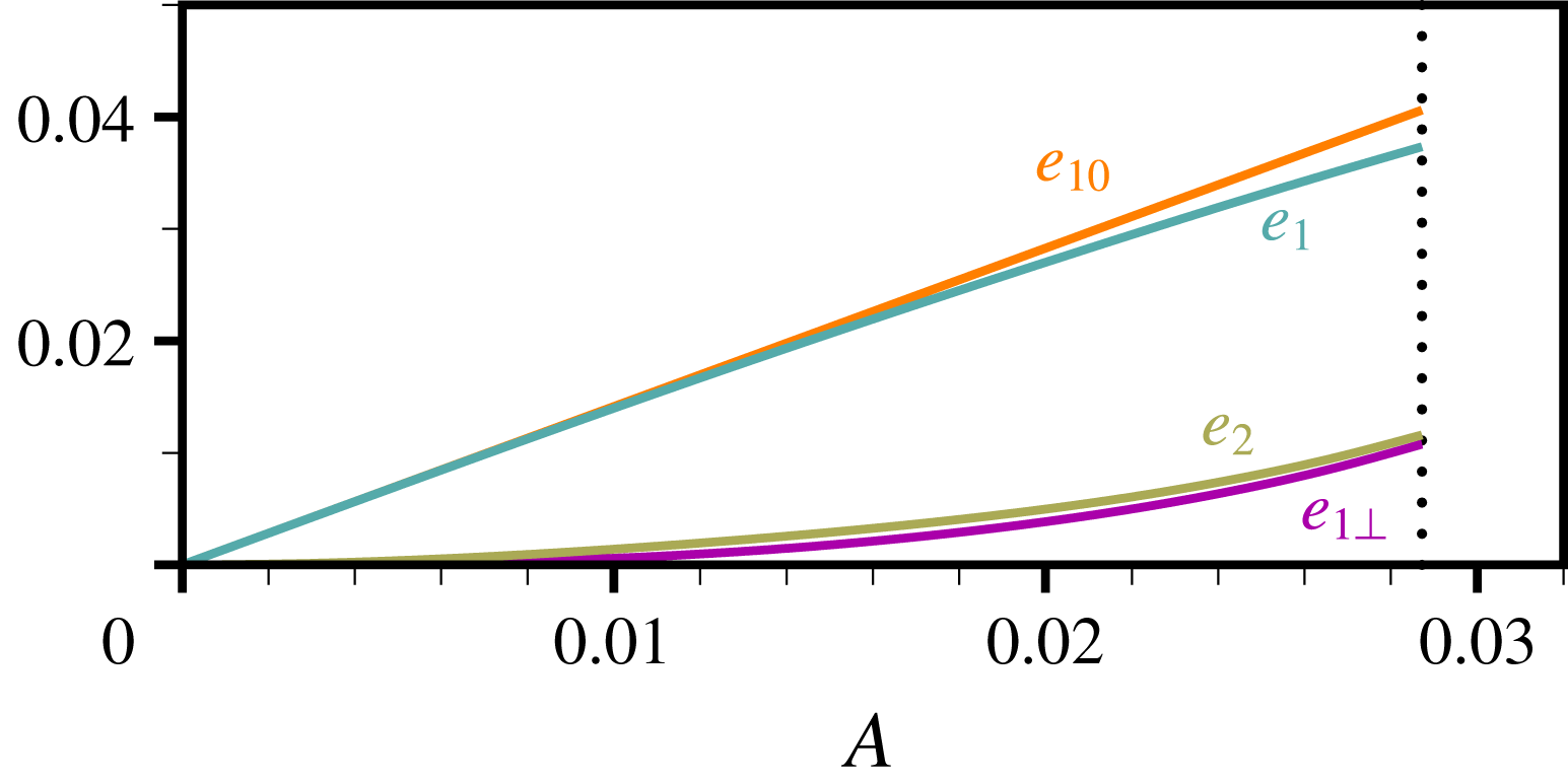
Phase-averaged mean oscillation amplitude of the leading eigenmode,
 $e_{10}=\sqrt{2}A\Vert \hat{\boldsymbol{u}}_{10}\Vert$
, of the orthogonal component,
 $e_{1\bot }=\sqrt{2}A\Vert \boldsymbol{u}_{1\bot }\Vert$
, of the first harmonic
 $e_{1}=\sqrt{2}A\Vert \hat{\boldsymbol{u}}_{10}+\boldsymbol{u}_{1\bot }\Vert$
and of the second harmonic
 $e_{2}=\sqrt{2}A\Vert \boldsymbol{u}_{2}\Vert$
. All amplitudes are measured by the root-mean-square of the corresponding fluctuating energy, and obtained by solving the self-consistent system (4.13) for increasing values of the amplitude
 $A$
; here
 $Re=6000$
.

(a) Linear growth rate
 $\unicode[STIX]{x1D70E}_{0}$
of the leading eigenmode and growth rate
 $\unicode[STIX]{x1D70E}$
of the first harmonic, as obtained by solving the self-consistent system (4.13) for increasing values of the amplitude
 $A$
. (b) Same as (a) for the eigenfrequency
 $\unicode[STIX]{x1D714}_{0}$
of the leading eigenmode and the oscillation frequency
 $\unicode[STIX]{x1D714}$
of the first harmonic; here
 $Re=6000$
.

Typical results obtained by solving system (4.13) at
 $Re=6000$
for increasing values of the amplitude are reported in figures 4 and 5. The amplitude of a given component is conveniently measured by the root-mean-square of its (phase-averaged) mean fluctuation energy, i.e.
 $e_{1}=\sqrt{2}A\Vert \boldsymbol{u}_{1}\Vert$
for the first harmonic,
 $e_{2}=\sqrt{2}A^{2}\Vert \boldsymbol{u}_{2}\Vert$
for the second harmonic, etc. Note that the obtained values are a priori mesh-dependent, but we have checked that computing all integrals on an inner domain defined arbitrarily as
 $(x,y)\in [-0.4,1.75]\times [-1,0.3]$
(dashed line in figure 1) produces identical values within
 $1.5\,\%$
. For
 $A=0$
, the mean flow reduces to the unstable base flow
 $\boldsymbol{u}_{b}$
and the structure of the first harmonic is given by the eigenmode
 $\hat{\boldsymbol{u}}_{10b}$
, whose growth rate
 $\unicode[STIX]{x1D70E}_{0b}=0.55$
and eigenfrequency
 $\unicode[STIX]{x1D714}_{0b}=10.69$
are those predicted by the linear theory. When
 $A$
increases, the leading eigenmode and the orthogonal component grow steadily (with
 $e_{10}>e_{1\bot }$
; see figure 4), and the harmonics follow suit (with
 $e_{1}>e_{2}$
, i.e. the first harmonic dominates even though
 $e_{1}^{}<e_{10}$
, because of the non-orthogonality of
 $\hat{\boldsymbol{u}}_{10}$
and
 $\boldsymbol{u}_{1\bot }$
). The growth rates
 $\unicode[STIX]{x1D70E}_{0}$
and
 $\unicode[STIX]{x1D70E}$
concurrently decrease while departing increasingly from each other (with
 $\unicode[STIX]{x1D70E}<\unicode[STIX]{x1D70E}_{0}$
; see figure 5), meaning that the base flow is progressively distorted into an increasingly stable mean flow. Meanwhile,
 $\unicode[STIX]{x1D714}_{0}$
and
 $\unicode[STIX]{x1D714}$
increase but remain close to each other (with
 $\unicode[STIX]{x1D714}\lesssim \unicode[STIX]{x1D714}_{0}$
). For
 $A=2.87\times 10^{-2}$
,
 $\unicode[STIX]{x1D70E}$
is exactly zero and the fluctuation (4.4) is purely harmonic, just like the saturated fluctuation of the DNS. The underlying mean flow is strongly linearly unstable with
 $\unicode[STIX]{x1D70E}_{0}=0.124$
, a value close to that,
 $\unicode[STIX]{x1D70E}_{0m}=0.117$
, obtained by linear stability analysis of the time-averaged mean flow. The frequency
 $\unicode[STIX]{x1D714}=11.21$
of the first harmonic is very close to that,
 $\unicode[STIX]{x1D714}_{nl}^{}=11.19$
, extracted from the DNS, but so is the leading eigenfrequency of the mean flow,
 $\unicode[STIX]{x1D714}_{0}=11.23$
, as further discussed in § 6.1.
The following picture comes out. In the linear regime, the first harmonic is parallel to the leading eigenmode
 $\hat{\boldsymbol{u}}_{10}$
. When nonlinearities set in, the self-interaction of
 $\hat{\boldsymbol{u}}_{10}$
generates a second harmonic
 $\boldsymbol{u}_{2}$
whose nonlinear interaction with the eigenmode feeds back and forces the growth of an orthogonal component
 $\boldsymbol{u}_{1\bot }$
. The latter distorts
 $\hat{\boldsymbol{u}}_{10}$
into an increasingly modified first harmonic
 $\boldsymbol{u}_{1}$
, while turning its linear growth rate
 $\unicode[STIX]{x1D70E}_{0}$
and eigenfrequency
 $\unicode[STIX]{x1D714}_{0}$
into
 $\unicode[STIX]{x1D70E}$
and
 $\unicode[STIX]{x1D714}$
. Both
 $\boldsymbol{u}_{1}$
and
 $\boldsymbol{u}_{2}$
feed back on the mean flow via their Reynolds stresses, and the growth rate of the first harmonic decreases, up to the point where it becomes exactly zero. At this stage, the base flow has been distorted into a strongly linearly unstable mean flow
 $(\unicode[STIX]{x1D70E}_{0}>0)$
, but perturbations stop growing and saturate because their linear growth is nonlinearly balanced by the stabilizing effect of the second harmonic. It is thus the distorted growth rate
 $\unicode[STIX]{x1D70E}=\unicode[STIX]{x1D70E}_{0}+\unicode[STIX]{x1D6FE}_{r}$
, not just the linear growth rate
 $\unicode[STIX]{x1D70E}_{0}$
, that is relevant to the mechanics of saturation. The oscillation frequency is similarly given by the distorted frequency
 $\unicode[STIX]{x1D714}=\unicode[STIX]{x1D714}_{0}+\unicode[STIX]{x1D6FE}_{i}$
, meaning that the eigenfrequency
 $\unicode[STIX]{x1D714}_{0}$
alone is not expected to be predictive, consistently with the argument of Sipp & Lebedev (Reference Sipp and Lebedev2007).
5 Comparison with results of direct numerical simulations
5.1 Saturated regime
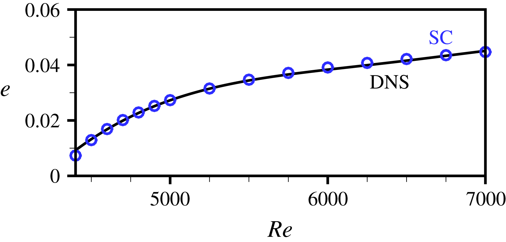
In the saturated regime, averaging over the phase is equivalent to averaging in time over a period of the oscillation; therefore the model predictions can be compared to time-averaged data from a single DNS. Here, the total self-consistent oscillation amplitude,
 $$\begin{eqnarray}e=\sqrt{e_{1}^{2}+e_{2}^{2}},\end{eqnarray}$$
shown in figure 6 is almost identical to its DNS counterpart
 $\overline{\Vert \boldsymbol{u}^{\prime }\Vert ^{2}}^{1/2}$
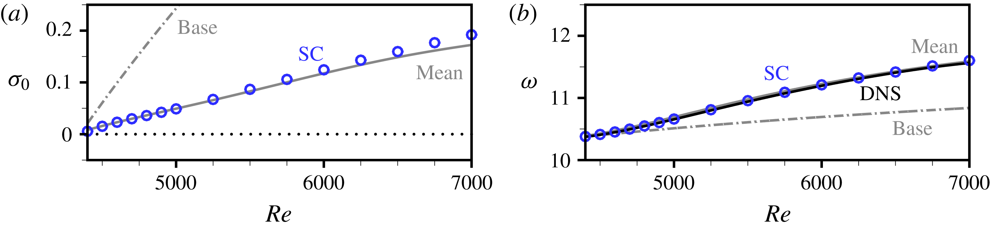
. Similarly, the linear growth rate
 $\unicode[STIX]{x1D70E}_{0}$
of the leading eigenmode and the oscillation frequency
 $\unicode[STIX]{x1D714}$
fall onto the values
 $\unicode[STIX]{x1D70E}_{0m}$
and
 $\unicode[STIX]{x1D714}_{nl}^{}$
extracted from the time-averaged mean flow; see figure 7.
Mean oscillation amplitude
 $e$
in the saturated regime against
 $Re$
: self-consistent (blue circles) versus DNS (black line).

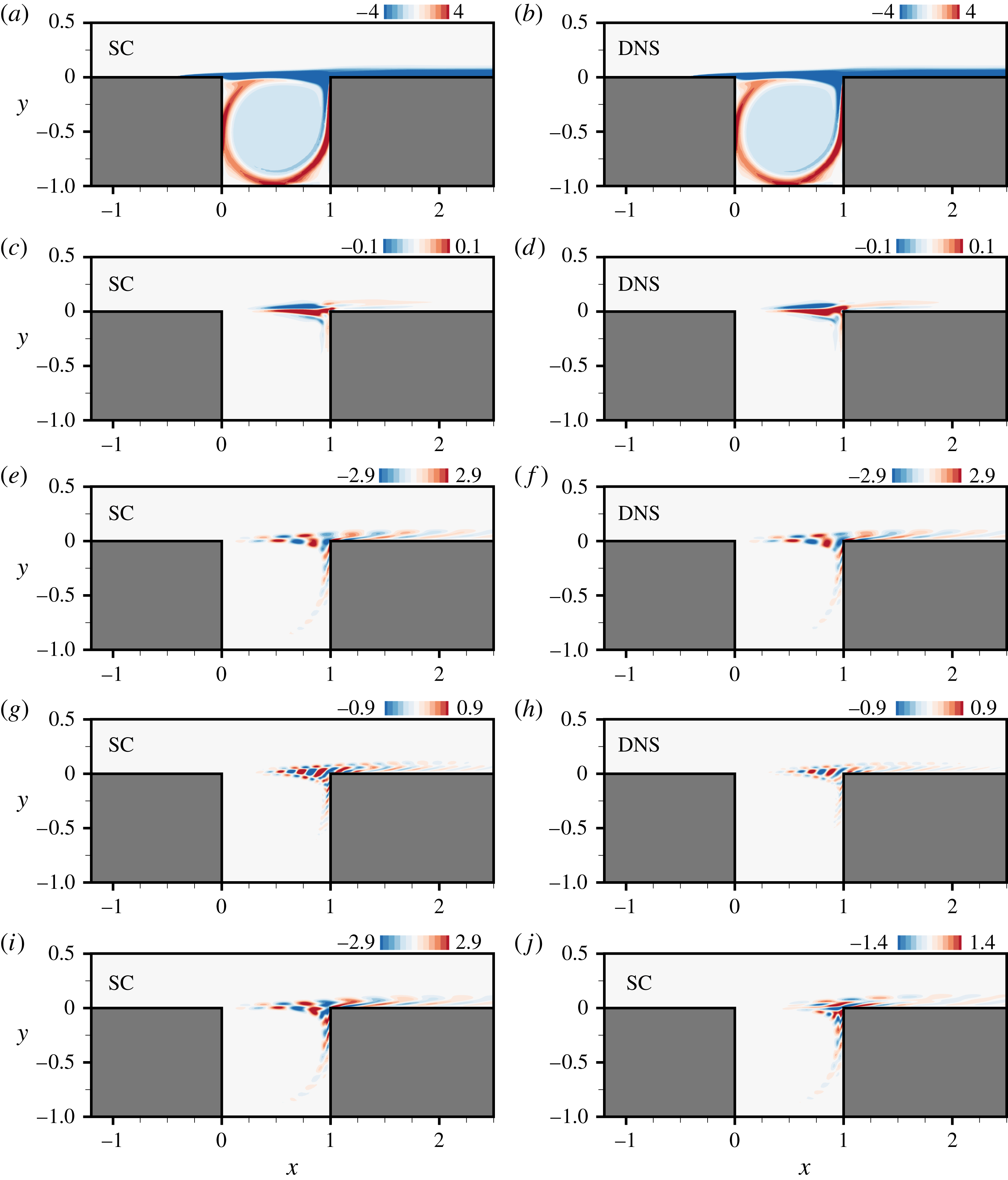
We show in figure 8(a,b) that the self-consistent mean flow
 $\langle \boldsymbol{u}\rangle$
reproduces remarkably well the time-averaged mean flow
 $\overline{\boldsymbol{u}}$
, and the same striking agreement is observed in figure 8(c,d) for the Reynolds stress divergence, calculated either from the model as
 $$\begin{eqnarray}A^{2}\unicode[STIX]{x1D74D}(\hat{\boldsymbol{u}}_{10}+\boldsymbol{u}_{1\bot })+A^{4}\unicode[STIX]{x1D74D}(\boldsymbol{u}_{2})\end{eqnarray}$$
or from the DNS as
 $\overline{\unicode[STIX]{x1D73B}(\boldsymbol{u}^{\prime })}$
. We also compare in figure 8(e–h) the self-consistent approximations of
 $\boldsymbol{u}_{1}$
and
 $\boldsymbol{u}_{2}$
to those harmonics obtained by performing a fast Fourier transform (FFT) of the instantaneous velocity at each point of the computational grid and retaining the terms at frequencies
 $\unicode[STIX]{x1D714}_{nl}^{}$
and
 $2\unicode[STIX]{x1D714}_{nl}^{}$
. For the first harmonic, the agreement is excellent, in terms of both magnitude and spatial distribution. At first sight, the structure resembles that of the leading eigenmode, whose self-consistent approximation
 $A\hat{\boldsymbol{u}}_{10}$
is documented in figure 8(i). There exist subtle differences, however, as the first harmonic precisely differs from the eigenmode by the orthogonal component
 $A\boldsymbol{u}_{1\bot }$
shown in figure 8(j), otherwise the cavity flow would comply with the linear marginal stability criterion. Locally, the magnitude of the orthogonal component can reach up to
 $50\,\%$
of that of the leading eigenmode, but its structure is more concentrated in the vicinity of the downstream edge, hence a ratio
 $e_{1\bot }/e_{10}\sim 25\,\%$
of the mean oscillation amplitudes, consistently with the results of figure 4. The spatial distribution of the second harmonic is also well predicted, but we notice a small discrepancy in magnitude, found to be slightly higher using the model. A possible explanation is that the FFT is performed over a time span of
 $100$
time units to avoid tremendous computational costs. This can alter the estimation of the higher Fourier coefficients, which is supported by the fact that the oscillation amplitude reconstructed from the first six FFT modes is lower by
 $6\,\%$
than the value documented in figure 6, obtained by averaging the DNS solution over
 $200$
time units.
Same as figure 6 for the (a) linear growth rate of the leading eigenmode and (b) the oscillation frequency. The results obtained by linear stability analysis of the time-averaged mean flow (respectively of the base flow) are shown by the grey line (respectively the dash-dotted grey line).

(a,b) Mean vorticity of the saturated cavity flow, as obtained by (a) solving the self-consistent system (4.13) and (b) averaging in time the instantaneous DNS solution. (c,d) Same as (a,b) for the
 $x$
-component of the Reynolds stress divergence. (e,f) Same as (a,b) for the first harmonic
 $A\boldsymbol{u}_{1}$
. (g,h) Same as (a,b) for the second harmonic
 $A^{2}\boldsymbol{u}_{2}$
. The fields in (f–h) have been obtained by FFT of the DNS solution and retaining the terms at frequencies
 $\unicode[STIX]{x1D714}_{nl}^{}$
and
 $2\unicode[STIX]{x1D714}_{nl}^{}$
. (i,j) Vorticity of the self-consistent (i) leading eigenmode
 $A\hat{\boldsymbol{u}}_{10}$
and (j) orthogonal component
 $A\boldsymbol{u}_{1\bot }$
. Here
 $Re=6000$
. Only the real part of a complex field is shown.

5.2 Transient regime
In the transient regime, the model predictions are compared to phase-averaged quantities computed from several DNS triggered by a different phase
 $\unicode[STIX]{x1D719}_{0}$
of the initial disturbance. We use here eight such values of
 $\unicode[STIX]{x1D719}_{0}$
uniformly distributed in
 $[0;2\unicode[STIX]{x03C0}]$
, which suffice to converge meaningful averages (it has been checked that identical results are obtained by using up to
 $16$
values), together with
 $A_{0}=5\times 10^{-6}$
as the controlled amplitude of the initial disturbance. It is easy to verify that the mean oscillation amplitudes
 $e_{1}$
and
 $e_{2}$
grow in time at rates
 $\unicode[STIX]{x1D70E}$
and
 $2\unicode[STIX]{x1D70E}$
, respectively. The quasi-static evolution of the self-consistent amplitude is thus determined by marching in time the equations
 $$\begin{eqnarray}\text{d}_{t}e_{1}=\unicode[STIX]{x1D70E}e_{1}\quad \text{and}\quad \text{d}_{t}e_{2}=2\unicode[STIX]{x1D70E}e_{2},\end{eqnarray}$$
from the knowledge of
 $\unicode[STIX]{x1D70E}(A)$
,
 $e_{1}(A)$
and
 $e_{2}(A)$
, following which (5.1) is used to recover the total amplitude. For the results to be comparable, we start from the initial condition
 $A(t=0)=\sqrt{2}A_{0}$
, and proceed with a fourth-order Runge–Kutta scheme, using polynomial interpolation at each time step to calculate
 $\unicode[STIX]{x1D70E}$
from the three closest neighbours.
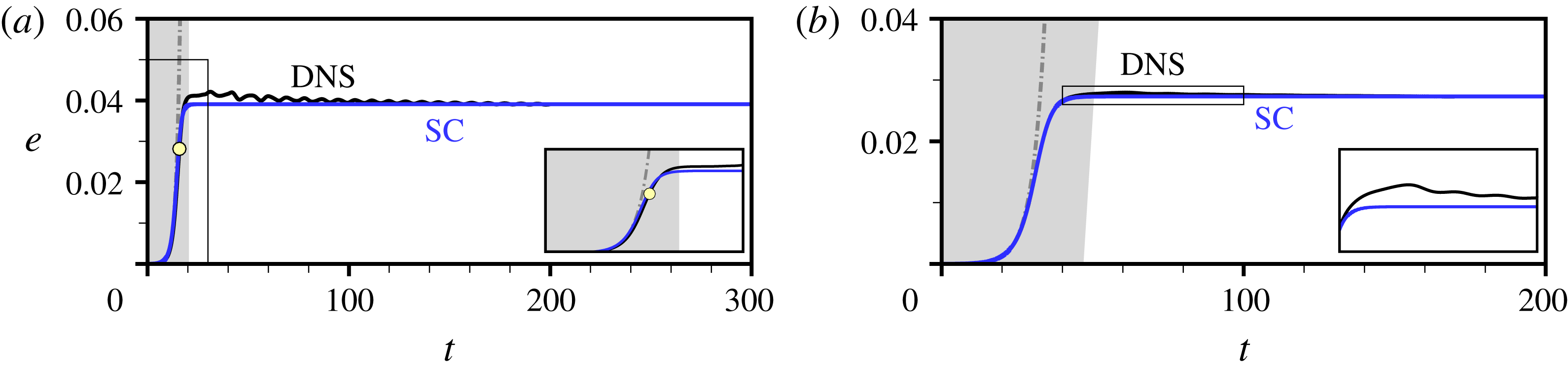
Transient evolution of the mean oscillation amplitude, as obtained by solving the self-consistent system (4.13) for various amplitudes and marching equations (5.3) in time (blue line), and averaging the instantaneous DNS solution over the phase of the initial perturbation (black line). The light grey shading marks the transient domain defined as the time interval for which the amplitude is less than
 $99\,\%$
of its saturated value. The grey dash-dotted line corresponds to the linear prediction of exponential growth at rate
 $\unicode[STIX]{x1D70E}_{0b}$
. (a) For
 $Re=6000$
. The yellow symbol marks the time
 $t=15.8$
for which figure 10 compares the model and exact mean flows. (b) For
 $Re=5000$
, together with a close-up on the overshoot region.

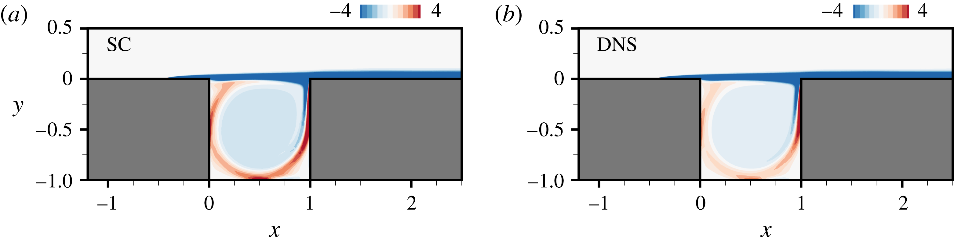
(a,b) Mean vorticity of the saturated cavity flow, as obtained by (a) solving the self-consistent system (4.13) for
 $A=2\times 10^{-2}$
, and (b) phase-averaging the instantaneous DNS solution at the corresponding time
 $t=15.8$
.

Figure 9(a) shows that the obtained self-consistent amplitude matches remarkably well the exact DNS value
 $\langle \Vert \boldsymbol{u}^{\prime }\Vert ^{2}\rangle ^{1/2}$
, up to
 $t=20$
where the amplitude has reached
 $99\,\%$
of its saturation value. This defines the length of the transient, as indicated by the light grey shading in figure 9(a), and completes the proof that the model properly captures the main mechanisms responsible for the transient growth and saturation of the instability. During the transient, the flow achieves almost
 $30$
flow oscillations (not shown here), which reasonably advocates the assumption about decoupling of scales made to derive the model. The nonlinearity becomes apparent midterm, at
 $t\sim 10$
, whereupon the self-consistent and DNS data deviate from the linear prediction of exponential growth at rate
 $\unicode[STIX]{x1D70E}_{0b}$
(grey dash-dotted line). Interestingly, there exist subtle differences in the dynamical paths taken by both solutions. For instance, we show in figure 10 that the self-consistent mean flow obtained for the amplitude
 $A=2\times 10^{-2}$
(which differs from the saturated solution by a lower magnitude of vorticity in the recirculating flow, and a thinner vorticity sheet close to the downstream edge) resembles a lot the DNS mean flow, phase-averaged at the corresponding time instant
 $t=15.8$
. The model, however, slightly overestimates the inner vorticity, which appears mandatory to better approximate the structure of the oscillation from the first two harmonics only.
Note that, for
 $20<t<30$
, the DNS data exhibit an overshoot that the self-consistent model fails to reproduce (probably because the quasi-static assumption is somehow faulty), whereupon the amplitude decreases while slowly oscillating towards its saturated value, reached at
 $t\sim 200$
. Such oscillations may reflect the destabilization of additional eigenmodes, as the base cavity flow undergoes a third Hopf bifurcation at
 $Re_{c3}=5698$
, but similar oscillations show up at
 $Re=5000$
, albeit with an amplitude so small that they are barely visible in figure 9(b). Another possibility is that the system amplifies the energy of the initial condition by non-normal mechanisms (Chomaz Reference Chomaz2005; Schmid Reference Schmid2007), which may cause transient, yet significant, mean flow distortions (Pralits, Bottaro & Cherubini Reference Pralits, Bottaro and Cherubini2015). Either way, the present model is meant to describe the growth of the sole bifurcating eigenmode, and is by construction unable to capture the mode interactions involved in these scenarios.
6 Discussion
6.1 Connection with weakly nonlinear analysis
There are several similarities (and also key differences) between the present approach and weakly nonlinear analyses meant to figure out the leading-order nonlinear effects associated with small-amplitude disturbances from the canonical Stuart–Landau amplitude
 $$\begin{eqnarray}d_{t}A=\unicode[STIX]{x1D706}\unicode[STIX]{x1D6E5}A-(\unicode[STIX]{x1D707}_{0}+\unicode[STIX]{x1D707}_{2})A|A|^{2},\end{eqnarray}$$
where
 $A$
is now the (complex) amplitude of the bifurcating eigenmode,
 $\unicode[STIX]{x1D6E5}=Re_{c}^{-1}-Re^{-1}$
measures the departure from the instability threshold,
 $\unicode[STIX]{x1D706}$
is the (complex) linear growth rate such that the leading eigenvalue is linearly approximated by
 $\text{i}\unicode[STIX]{x1D714}_{0b}(Re_{c})+\unicode[STIX]{x1D706}\unicode[STIX]{x1D6E5}$
, and
 $\unicode[STIX]{x1D707}_{0}$
(respectively
 $\unicode[STIX]{x1D707}_{2}$
) is the (complex) Landau coefficient determined by the nonlinear interaction of the eigenmode with the mean flow distortion induced by its Reynolds stresses (respectively with its second harmonic). All coefficients can be determined numerically by applying multiple time-scale analysis (Sipp & Lebedev Reference Sipp and Lebedev2007; Meliga, Chomaz & Sipp Reference Meliga, Chomaz and Sipp2009a
) at the second threshold of instability
 $Re_{c2}=4348$
(since we recall that the first two eigenmodes to bifurcate exchange dominance at
 $Re=4567$
). This yields
 $\unicode[STIX]{x1D706}=7689+4645\text{i}$
,
 $\unicode[STIX]{x1D707}_{0}=583.0-129.8\text{i}$
and
 $\unicode[STIX]{x1D707}_{2}=228.8+98.98\text{i}$
.
Weakly nonlinear analysis also invokes a scale separation argument (fast time scale for the flow oscillations versus slow time scale for the growth of the oscillation amplitude) to derive (6.1) from a hierarchy of equations at various orders in a small parameter, physically representing the order of magnitude of the flow disturbances. However, the time-averaged mean oscillation amplitude computed from the (real) limit-cycle amplitude,
 $$\begin{eqnarray}|A|=\sqrt{\frac{\unicode[STIX]{x1D706}_{r}\unicode[STIX]{x1D6E5}}{\unicode[STIX]{x1D707}_{0r}+\unicode[STIX]{x1D707}_{2r}}},\end{eqnarray}$$
departs rapidly from the DNS and self-consistent data for
 $Re\gtrsim 4600$
. This is because the aforementioned asymptotic hierarchy of equations becomes invalid when the size of the disturbances becomes large enough for nonlinearities to set in. There is no such hierarchy in self-consistent modelling, where the fluctuation is built as successive-order corrections to the leading eigenmode of the mean flow, and all effects are encompassed rigorously regardless of their orders of magnitude; hence the ability to support an arbitrary level of supercriticality.
Valuable insights can still be gained from weakly nonlinear analysis. For instance, the above values of
 $\unicode[STIX]{x1D707}_{0r}$
and
 $\unicode[STIX]{x1D707}_{2r}$
indicate that both the mean flow distortion induced by the Reynolds stresses of the leading eigenmode and the second harmonic are stabilizing (
 $\unicode[STIX]{x1D707}_{0r}>0$
and
 $\unicode[STIX]{x1D707}_{2r}>0$
), and it can be inferred that both mechanisms contribute to saturate the instability since
 $\unicode[STIX]{x1D707}_{2r}/\unicode[STIX]{x1D707}_{0r}=O(1)$
. This is true also of the present self-consistent results: in the absence of a second harmonic, the stabilizing effect of the Reynolds stresses is evidenced by the mean flow becoming increasingly linearly stable when solving the self-consistent system of Mantič-Lugo et al. (Reference Mantič-Lugo, Arratia and Gallaire2014) for increasing values of the amplitude
 $A_{sc1}$
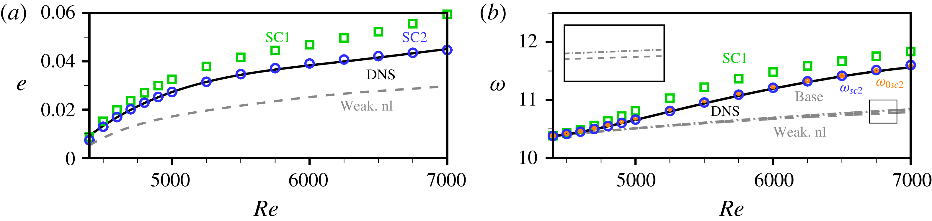
(not shown here). As for the stabilizing effect of the second harmonic, it shows in figure 11(b) through the fact that the amplitude
 $A_{sc2}$
obtained with the present model is systematically smaller than
 $A_{sc1}$
, just like the amplitude (6.2) is systematically smaller than that,
 $|A_{0}|=\sqrt{\unicode[STIX]{x1D706}_{r}\unicode[STIX]{x1D6E5}/\unicode[STIX]{x1D707}_{0r}}$
, obtained by retaining only the mean flow distortion.
(a) Mean oscillation amplitude in the saturated regime against
 $Re$
: second-order self-consistent (blue circles) versus first-order self-consistent (green squares) versus DNS (black line) versus weakly nonlinear analysis (grey dashed line). (b) Same as (a) for the oscillation frequency. The second-order self-consistent results feature both the nonlinear oscillation frequency
 $\unicode[STIX]{x1D714}$
(blue circles), and the mean flow eigenfrequency
 $\unicode[STIX]{x1D714}_{0}$
(smaller orange dots). The value obtained by linear stability analysis of the base flow is shown as the grey dash-dotted line.

The weakly nonlinear limit-cycle frequency is given by
 $$\begin{eqnarray}\unicode[STIX]{x1D714}_{wnl}-\unicode[STIX]{x1D714}_{0b}=-\frac{\unicode[STIX]{x1D707}_{0i}+\unicode[STIX]{x1D707}_{2i}}{\unicode[STIX]{x1D707}_{0r}+\unicode[STIX]{x1D707}_{2r}}\unicode[STIX]{x1D706}_{r}\unicode[STIX]{x1D6E5}=\underbrace{-\unicode[STIX]{x1D707}_{0i}|A_{0}|^{2}}_{\text{(i)}}\underbrace{-\unicode[STIX]{x1D707}_{0i}(|A|^{2}-|A_{0}|^{2})}_{\text{(ii)}}\underbrace{-\unicode[STIX]{x1D707}_{2i}|A|^{2}}_{\text{(iii)}}.\end{eqnarray}$$
The nonlinear frequency correction on the RHS brings out three contributions: (i) due to the mean flow distortions induced by the Reynolds stresses of the leading eigenmode; (ii) due to the second harmonic changing the amplitude of the Reynolds stresses from
 $|A_{0}|^{2}$
to
 $|A|^{2}$
; and (iii) due to the nonlinear interaction between the second harmonic and the leading eigenmode. The above values of
 $\unicode[STIX]{x1D707}_{0i}$
and
 $\unicode[STIX]{x1D707}_{2i}$
suggest that the mean flow distortion increases the frequency (
 $\unicode[STIX]{x1D707}_{0i}<0$
). The stabilizing effect of the second harmonic tends to decrease it (
 $|A|<|A_{0}|$
), while the nonlinear interaction between harmonics yields additional frequency reduction (
 $\unicode[STIX]{x1D707}_{2i}>0$
). Quite fortuitously, all three effects balance each other almost exactly because
 $|\unicode[STIX]{x1D707}_{0i}+\unicode[STIX]{x1D707}_{2i}|/|\unicode[STIX]{x1D707}_{0r}+\unicode[STIX]{x1D707}_{2r}|\ll 1$
; hence the weakly nonlinear frequency is almost identical to the leading eigenfrequency of the base flow
 $\unicode[STIX]{x1D714}_{0b}$
, as can be seen by comparing the grey dashed and dash-dotted lines in figure 11(b). We insist that the nonlinearity itself is significant, otherwise the weakly nonlinear frequency would fall onto the self-consistent and DNS data regardless of the value of
 $Re$
. These interpretations essentially carry over to the strongly nonlinear regime provided the self-consistent frequency
 $\unicode[STIX]{x1D714}_{sc2}^{}$
is recast into
 $$\begin{eqnarray}\unicode[STIX]{x1D714}_{sc2}^{}-\unicode[STIX]{x1D714}_{0b}^{}=(\unicode[STIX]{x1D714}_{0sc2}^{}-\unicode[STIX]{x1D714}_{0sc1}^{})+(\unicode[STIX]{x1D714}_{0sc1}^{}-\unicode[STIX]{x1D714}_{0b}^{})+\unicode[STIX]{x1D6FE}_{i},\end{eqnarray}$$
where
 $\unicode[STIX]{x1D714}_{0sc1}^{}=\unicode[STIX]{x1D714}_{sc1}^{}$
is the mean flow eigenfrequency predicted by the first-order model of Mantič-Lugo et al. (Reference Mantič-Lugo, Arratia and Gallaire2014). The mean flow distortion induced by the Reynolds stresses of the leading eigenmode is seen in figure 11(b) to increase the oscillation frequency (
 $\unicode[STIX]{x1D714}_{0sc1}^{}>\unicode[STIX]{x1D714}_{0b}^{}$
). The modification of the Reynolds stresses induced by the second harmonic conversely decreases it (
 $\unicode[STIX]{x1D714}_{0sc1}^{}>\unicode[STIX]{x1D714}_{0sc2}^{}$
), which is similar to the interpretation of the Landau coefficients, although we reiterate that the physics captured by weakly nonlinear analysis on this is very limited. Finally, the nonlinear interaction of the harmonics with the leading eigenmode yields additional frequency reduction for
 $Re<6500$
(
 $\unicode[STIX]{x1D714}_{sc2}^{}\lesssim \unicode[STIX]{x1D714}_{0sc2}^{}$
) but conversely an additional frequency increase for
 $Re>6500$
(
 $\unicode[STIX]{x1D714}_{sc2}^{}\gtrsim \unicode[STIX]{x1D714}_{0sc2}^{}$
). This is barely visible in figure 11(b) because of the smallness of the frequency detuning
 $\unicode[STIX]{x1D6FE}_{i}$
, which explains why the mean flow eigenfrequency ends up doing well on the frequency prediction. Anyhow, this is likely to be fortuitous, as Turton et al. (Reference Turton, Tuckerman and Barkley2015) report specific regimes of thermosolutal convection in which the eigenfrequency is not predictive, which we infer is because the related value of
 $\unicode[STIX]{x1D6FE}_{i}$
is
 $O(1)$
.
The nonlinearity at play in a given flow can be identified from the linear stability properties of the time-averaged mean flow: a strongly linearly unstable leading eigenmode or one whose eigenfrequency approximates poorly the nonlinear frequency reflects both mean flow distortions and generation of higher-order harmonics. In this case, the main features of the related oscillation are best predicted using a multi-order model to encompass the
 $O(1)$
value of the underlying detuning parameter. A leading eigenmode close to marginal linear stability and whose eigenfrequency approximates well the nonlinear frequency conversely reflects pure mean flow distortions, in which case relevant predictions can be obtained with the model of Mantič-Lugo et al. (Reference Mantič-Lugo, Arratia and Gallaire2014) because the detuning parameter is close to zero. Both conditions are required, as the present cavity flow serves as a reminder that the mean flow eigenfrequency can quite fortuitously predict the nonlinear frequency, if
 $\unicode[STIX]{x1D6FE}_{i}\ll 1$
, even though the nonlinearity is not restricted to mean flow distortion, if
 $\unicode[STIX]{x1D6FE}_{r}=O(1)$
. This generalizes the distinction introduced by Sipp & Lebedev (Reference Sipp and Lebedev2007) in their analysis of the amplitude equation, the weakly nonlinear equivalent of the present model being an amplitude equation with
 $|\unicode[STIX]{x1D707}_{2}|/|\unicode[STIX]{x1D707}_{0}|=O(1)$
, while that of the model of Mantič-Lugo et al. (Reference Mantič-Lugo, Arratia and Gallaire2014) is an amplitude equation with
 $|\unicode[STIX]{x1D707}_{2}|/|\unicode[STIX]{x1D707}_{0}|\ll 1$
.
6.2 Effect of the truncation order
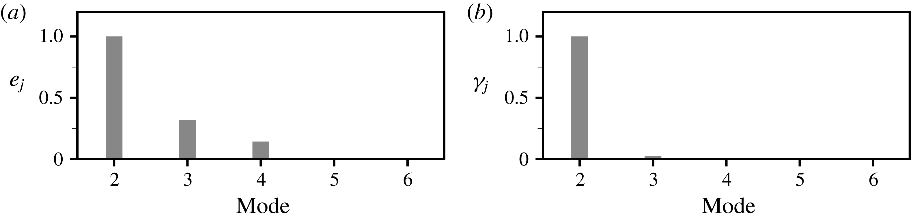
Caution should be used in generalizing the present results to other cases involving significant generation of higher harmonics. If the flow is not within the scope of the first-order model, then we expect a valuable (albeit incomplete) description of the main nonlinear mechanisms at play to be obtained from a second-order model. Still, higher-order Fourier expansions of the fluctuation may be necessary to obtain more accurate, quantitative predictions, which requires the model to be augmented with linear equations for the higher harmonics forced by relevant nonlinear terms describing the interactions of the lower harmonics. In this eventuality, an interesting point to discuss is whether or not it is possible to anticipate the proper number of harmonics to be retained. Spectra can be useful to unravel the existence (or the absence) of harmonics, but they are not very insightful for the intended purpose because they give only a local, partial vision of the nonlinearity. For instance, velocity spectra measured in the recirculating flow unveil essentially a single peak at the fundamental frequency (not shown here), which merely reflects the low magnitude of the second harmonic in this specific flow region; see figure 8. While a more global perspective is achieved by resorting to FFT to extract the structure of the various harmonics (as has been done for the first and second harmonics in § 5.1), it may not be relevant to rest on the sole oscillation amplitude
 $e_{j}=\Vert \boldsymbol{u}_{j}\Vert$
, as we show in figure 12(a) that the amplitude of the third (and even the fourth) mode of the cavity is not necessarily obviously negligible. This is because the nonlinear correction induced by the higher-order harmonic via the detuning parameter
 $\unicode[STIX]{x1D6FE}$
depends not only on the structure of the harmonics, but also on their recombination via the advection operator (which yields the forcing terms acting at each frequency) and on the orientation of these forces with respect to the adjoint eigenmode. Assuming that
 $n$
harmonics are available from the FFT, the definition (4.13f
) of the detuning parameter generalizes easily to
 $$\begin{eqnarray}\unicode[STIX]{x1D6FE}=\mathop{\sum }_{j=2}^{n}\unicode[STIX]{x1D6FE}_{j},\quad \text{with }\unicode[STIX]{x1D6FE}_{j}=-\frac{(\hat{\boldsymbol{u}}_{10}^{\dagger }\mid \unicode[STIX]{x1D753}(\boldsymbol{u}_{j-1}^{\ast },\boldsymbol{u}_{j}))}{(\hat{\boldsymbol{u}}_{10}^{\dagger }\mid \boldsymbol{u}_{1})},\end{eqnarray}$$
where each individual detuning
 $\unicode[STIX]{x1D6FE}_{j}$
accounts for additional distortions to the linear growth rate and eigenfrequency of the leading eigenmode induced by the
 $j$
-th harmonic. We have computed the individual detuning coefficients of the first six FFT modes, using the leading adjoint eigenmode of the time-averaged mean flow to evaluate numerically all inner products. The results shown in figure 12(b) clearly stress that only the contribution
 $\unicode[STIX]{x1D6FE}_{2}$
of the second harmonic needs to be retained, with marginal correction of the third harmonic, and no effect of the higher-order harmonics. This is as close as one can get to identify a relevant order of truncation without any input from the self-consistent model.
(a) Amplitude
 $e_{j}$
of the first six harmonics, as obtained by FFT of the DNS solution. (b) Contribution
 $\unicode[STIX]{x1D6FE}_{j}$
of each mode to the detuning parameter, as defined by (6.5). Here
 $Re=6000$
. All results normalized for the second harmonic to peak at unity.

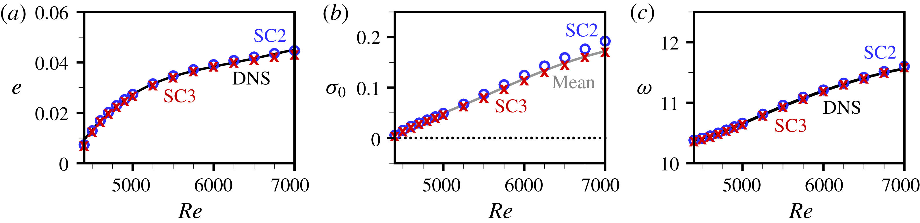
As a proof of feasibility (and also as an attempt to assess the relevance of the above criterion), we show in figure 13 that all values obtained by solving the third-order self-consistent model are almost identical to those presented above, hence confirming that the second-order results come with little to no truncation effect. Of course, the computational cost increases with the order of the model because an inner loop needs to be added in the iterative algorithm for the computation of each additional harmonic (hence three nested loops for the third-order model, and so on). For our case, converging the third harmonic to the same precision yields an increase in the number of iterations by roughly
 $30\,\%$
. Finding ways to improve the numerical resolution of the self-consistent equations in the foreseeable future is thus a major stake, as increasing the number of harmonics may be a much needed step towards extending the scope of the method to more complex turbulent regimes.
(a) Mean oscillation amplitude in the saturated regime against
 $Re$
: second-order self-consistent (blue circles) versus third-order self-consistent (red crosses) versus DNS (black line). (b,c) Same as (a) for (b) the linear growth rate of the leading eigenmode and (c) the oscillation frequency. The grey line in (b) is the value obtained by linear stability analysis of the time-averaged mean flow.

6.3 Concluding remarks
The present model provides a consistent picture of the saturation process in unsteady flows whose nonlinearity involves not only mean flow distortions but also production of higher harmonics. Saturation occurs when the growth rate of the first harmonic is zero, at which point the second harmonic balances exactly the non-zero linear growth rate of the leading eigenmode. This rationalizes the existence of strongly linearly unstable mean flows, and paves the way for new analysis techniques of such flows, including model reduction and flow control, just like the model of Mantič-Lugo et al. (Reference Mantič-Lugo, Arratia and Gallaire2014) did for systems whose mean flow is linearly marginally stable (Meliga et al. Reference Meliga, Boujo and Gallaire2016a ). It is worth noticing that the relevance of this type of model, in which perturbation equations are linearized around a mean flow determined simultaneously from the Reynolds stress of the perturbations, goes well beyond limit cycles. In particular, we expect the method to be capable of tackling extrinsic unsteady dynamics, for which a first step has been taken by Mantič-Lugo & Gallaire (Reference Mantič-Lugo and Gallaire2016) using their first-order model. Also, several papers in the recent literature have used similar coupled models retaining the Reynolds stresses of transiently unstable linear and weakly nonlinear disturbances to explain the emergence of coherent structure in otherwise linearly stable, parallel shear flows (Farrell & Ioannou Reference Farrell and Ioannou2012; Beaume et al. Reference Beaume, Chini, Julien and Knobloch2015; Pralits et al. Reference Pralits, Bottaro and Cherubini2015; Farrell et al. Reference Farrell, Ioannou, Jiménez, Constantinou, Lozano-Durán and Nikolaidis2016).
Acknowledgements
This work is supported by the ‘Investissements d’Avenir’ French Government programme, managed by the French National Research Agency (ANR) through the A*MIDEX grant (ANR-11-IDEX-0001-02) and the LABEX MEC project (ANR-11-LABX-0092).