1. Introduction
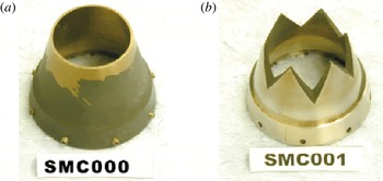
Jet noise is a concern for the continued expansion of aviation, and several passive and active control techniques are being researched to address the issue. One such solution that has been actually deployed on production aircraft is the addition of serrations called chevrons at the nozzle trailing edge (see figure 1). The chevron tips impinge on the jet shear layer and generate streamwise vortices that enhance mixing and shorten the potential core (Bridges & Brown Reference Bridges and Brown2004; Alkislar, Krothapalli & Butler Reference Alkislar, Krothapalli and Butler2007). In fact, the time-averaged jet cross-section becomes serrated corresponding to the chevrons on the nozzle. The nozzle serrations reduce the low-frequency mixing noise at aft angles (the loudest component of jet noise), but typically increase high-frequency noise at all angles (Bridges & Brown Reference Bridges and Brown2004).
Round (a) and serrated (b) nozzles (among many) evaluated in experiments by Bridges & Brown (Reference Bridges and Brown2004).

The low-frequency aft-angle mixing noise in round jets has been linked with the kinematics of large-scale coherent structures within the turbulent jet plume, as reviewed recently by Jordan & Colonius (Reference Jordan and Colonius2013). The convecting coherent fluctuations appear as wavepackets in narrow-band-frequency-filtered two-point cross correlations, especially in the irrotational near pressure field, as observed first by Mollo-Christensen (Reference Mollo-Christensen1967). The low-frequency wavepackets display significant coherence over streamwise domains that are several times the nozzle exit diameter. Such observations have since prompted many attempts at modelling turbulent coherent structures as linear instability modes of the time-averaged flow field – the Kelvin–Helmholtz instability. As examples, we cite the works of Crighton & Gaster (Reference Crighton and Gaster1976), Mankbadi & Liu (Reference Mankbadi and Liu1984), Tam & Burton (Reference Tam and Burton1984) and Goldstein & Leib (Reference Goldstein and Leib2005). Recent rigorous validations, made possible by the current availability of detailed experimental data and well-validated large-eddy simulation (LES) databases, have leant renewed credence to the linear stability model (Jordan & Colonius Reference Jordan and Colonius2013). Cavalieri et al. (Reference Cavalieri, Rodríguez, Jordan, Colonius and Gervais2013) also provide empirical support for the assumption of linearity of the low-frequency low-azimuthal mode turbulent fluctuations, which are responsible for most of the mixing noise due to their high coherence.
The models for coherent fluctuations in round jets have been constructed both from the classical parallel-flow linear stability theory (LST) (e.g. Suzuki & Colonius Reference Suzuki and Colonius2006) and the parabolized stability equation (PSE). PSE represents an improvement over LST whereby mildly non-parallel base flows in convectively unstable flows (like jets) can be addressed at little additional computational cost (Herbert Reference Herbert1997). The instability wave ansatz is allowed to have slow streamwise variations in shape, growth rate and phase speed of the order of the variations in the mean flow. Suitable numerical considerations (Li & Malik Reference Li and Malik1997) then allow the solution to be marched downstream. Linear PSE has been applied successfully to predict the coherent wavepackets extracted from data of round jets, both subsonic and supersonic (Gudmundsson & Colonius Reference Gudmundsson and Colonius2011; Cavalieri et al. Reference Cavalieri, Rodríguez, Jordan, Colonius and Gervais2013; Sinha et al. Reference Sinha, Rodríguez, Brès and Colonius2014).
Based on the previous modelling success in round jets, we pursue herein the modelling of the low-frequency low-azimuthal mode coherent wavepackets observed in turbulent jets issuing from serrated nozzles with PSE. These calculations are initiated near the nozzle with the LST solution, so that the latter are also described. The LST problem for round jets is one-dimensional – only the radial direction is inhomogeneous. The major point of difference of the LST problem for jets issuing from serrated nozzles is its two-dimensionality, given that the azimuthal direction is also inhomogeneous. Kawahara et al. (Reference Kawahara, Jiménez, Uhlmann and Pinelli2003) studied the inviscid temporal LST for a corrugated vortex sheet with application to boundary-layer stability. Gudmundsson & Colonius (Reference Gudmundsson and Colonius2007) were the first to solve the inviscid spatial LST problem for serrated jets, wherein they explicitly used the azimuthal regularity of the serrations to substantially simplify and elucidate the theory. In particular, they showed that the two-dimensional eigenproblem reduces to a set of coupled Rayleigh equations in one (radial) dimension. Our approach in LST hews closely to this earlier work, but we extend it to the viscous problem. The same framework is also extended to the PSE calculations for tracking the downstream evolution of the unstable wavepackets. In particular, the normally three-dimensional PSE problem for serrated jets is simplified to a coupled set of two-dimensional ones. Recently, Uzun et al. (Reference Uzun, Alvi, Colonius and Hussaini2015) revisited the two-dimensional version of the inviscid LST and the three-dimensional version of the inviscid PSE problem for serrated jets. Our formulation here allows significant simplification but is otherwise equivalent, except for viscous effects. The closeness of our mutual stability results reflects the minor role that viscosity plays in the problem.
Apart from the above-mentioned theoretical advances made in the present work, the other major contribution is a detailed validation of the model predictions using empirical data. The time-averaged flow data for the stability calculations come from the parametric experiments of Bridges & Brown (Reference Bridges and Brown2004), who also acquired the near-field hydrodynamic pressure on a phased array since it reveals the wavepacket nature of the shear-layer fluctuations most clearly (Suzuki & Colonius Reference Suzuki and Colonius2006; Jordan & Colonius Reference Jordan and Colonius2013). Following Gudmundsson & Colonius (Reference Gudmundsson and Colonius2011), the pressure data is filtered with proper orthogonal decomposition (POD) to extract the coherent wavepackets existing in the turbulence, which are then used to validate the stability results. Another novel comparison pursued here is with an LES database of the same serrated jet (Xia, Tucker & Eastwood Reference Xia, Tucker and Eastwood2009; Xia & Tucker Reference Xia and Tucker2012). The pressure component of this data (extracted in a cylindrical domain containing the jet plume) is also POD-filtered to identify the wavepacket structure within the shear layer. Reasonable agreement is demonstrated in both validation exercises, which lends confidence to the proposed PSE-based model for coherent wavepackets in serrated jets.
2. Linear parabolized stability equations for serrated jets
The flow field of the jet is described in cylindrical coordinates
 $\boldsymbol{x}=(x,r,{\it\theta})$
by
 $\boldsymbol{q}=(u_{x},u_{r},u_{{\it\theta}},p,{\it\zeta})^{\text{T}}$
, which respectively denote the axial, radial and azimuthal components of velocity, pressure, and specific volume. Length dimensions are non-dimensionalized by the nozzle exit diameter
 $D$
, velocities by the ambient speed of sound
 $c_{\infty }$
, and pressure by
 ${\it\rho}_{\infty }c_{\infty }^{2}$
(
 ${\it\rho}_{\infty }$
is the ambient density). PSE starts by decomposing
 $\boldsymbol{q}$
into a time-invariant base flow (herein the turbulent mean flow)
 $\overline{\boldsymbol{q}}$
, and the residual fluctuations
 $\boldsymbol{q}^{\prime }$
. The set of five non-dimensional governing equations for the viscous compressible flow linearized about
 $\overline{\boldsymbol{q}}$
, are compactly represented in matrix form as
 $$\begin{eqnarray}\left\{\overline{\unicode[STIX]{x1D647}}^{0}+\overline{\unicode[STIX]{x1D647}}^{t}\frac{\partial }{\partial t}+\overline{\unicode[STIX]{x1D647}}^{x}\frac{\partial }{\partial x}+\overline{\unicode[STIX]{x1D647}}^{r}\frac{\partial }{\partial r}+\overline{\unicode[STIX]{x1D647}}^{{\it\theta}}\frac{\partial }{\partial {\it\theta}}+\mathop{\sum }_{{\it\sigma},{\it\tau}\in \{x,r,{\it\theta}\}}\overline{\unicode[STIX]{x1D647}}^{{\it\sigma}{\it\tau}}\frac{\partial ^{2}}{\partial {\it\sigma}\partial {\it\tau}}\right\}\boldsymbol{q}^{\prime }=\mathbf{0}.\end{eqnarray}$$
The
 $5\times 5$
coefficient matrices
 $\overline{\unicode[STIX]{x1D647}}$
are linear functions of
 $\overline{\boldsymbol{q}}$
, and are parametrized by the Reynolds number, Mach number and Prandtl number of the flow.
Since
 $\overline{\unicode[STIX]{x1D647}}$
’s are time invariant, the solution is separable into its frequency components (normal modes). Moreover,
 $\overline{\boldsymbol{q}}$
is assumed to have gradual variations in the axial direction. With this, the preliminary PSE ansatz for
 $\boldsymbol{q}^{\prime }$
in the serrated mean flow field is
 $$\begin{eqnarray}\boldsymbol{q}^{\prime }(\boldsymbol{x},t)=\hat{\boldsymbol{q}}_{{\it\omega}}(\boldsymbol{x})\text{e}^{-\text{i}{\it\omega}t}+\text{c.c.},\quad \hat{\boldsymbol{q}}_{{\it\omega}}(\boldsymbol{x})=\mathscr{B}_{{\it\omega}}\underbrace{\text{e}^{\text{i}\int _{x_{0}}^{x}{\it\alpha}_{{\it\omega}}({\it\xi})\,\text{d}{\it\xi}}}_{=:{\it\chi}_{{\it\omega}}}\mathop{\sum }_{m=-\infty }^{\infty }\tilde{\boldsymbol{q}}_{{\it\omega},m}(x,r)\text{e}^{\text{i}m{\it\theta}}.\end{eqnarray}$$
Here, the symbol
 $m$
is the Fourier azimuthal mode. The frequency
 ${\it\omega}$
will be reported subsequently in terms of the Strouhal number
 $St$
based on the nozzle exit velocity
 $U_{j}$
and diameter
 $D$
. Further,
 $\tilde{\boldsymbol{q}}_{{\it\omega},m}$
is the wavepacket shape function and
 ${\it\alpha}_{{\it\omega}}$
is its complex axial wavenumber, both assumed to have mild axial variation (commensurate with the mildly non-parallel base flow), on scales that are significantly longer than the modal wavelength. The real and imaginary parts of
 ${\it\alpha}_{{\it\omega}}$
, denoted
 ${\it\alpha}_{{\it\omega}}^{r}$
and
 ${\it\alpha}_{{\it\omega}}^{i}$
, signify the local wavenumber and growth rate, respectively. For later convenience, we denote the wave part of the solution by
 ${\it\chi}_{{\it\omega}}$
. The complex amplitude of the wavepacket is set by
 $\mathscr{B}_{{\it\omega}}$
.
The nozzles typically have
 $L$
chevrons distributed uniformly around the azimuth (e.g.
 $L=6$
for SMC001 in figure 1). The resulting mean flow field has an
 $L$
-fold rotational symmetry so that the
 $m$
th azimuthal Fourier mode of
 $\overline{\boldsymbol{q}}$
(denoted
 $\check{\overline{\boldsymbol{q}}}_{m}$
) vanishes for all
 $m$
that are not integer multiples of
 $L$
:
 $$\begin{eqnarray}\overline{\boldsymbol{q}}(x,r,{\it\theta})=\mathop{\sum }_{j=-\infty }^{\infty }\check{\overline{\boldsymbol{q}}}_{Lj}(x,r)\text{e}^{\text{i}Lj{\it\theta}}.\end{eqnarray}$$
Substituting the foregoing ansatz in the linearized governing equations (2.1), we obtain
 $$\begin{eqnarray}\displaystyle & & \displaystyle \mathop{\sum }_{j=-\infty }^{\infty }\left[\left\{\check{\overline{\unicode[STIX]{x1D647}}}_{Lj}^{0}-\text{i}{\it\omega}\check{\overline{\unicode[STIX]{x1D647}}}^{t}+\check{\overline{\unicode[STIX]{x1D647}}}_{Lj}^{r}\frac{\partial }{\partial r}+\check{\overline{\unicode[STIX]{x1D647}}}_{Lj}^{rr}\frac{\partial ^{2}}{\partial r^{2}}\right.\right.\nonumber\\ \displaystyle & & \displaystyle \quad +\left.\text{i}(m-Lj)\left(\check{\overline{\unicode[STIX]{x1D647}}}_{Lj}^{{\it\theta}}+\check{\overline{\unicode[STIX]{x1D647}}}_{Lj}^{r{\it\theta}}\frac{\partial }{\partial r}\right)-(m-Lj)^{2}\check{\overline{\unicode[STIX]{x1D647}}}_{Lj}^{{\it\theta}{\it\theta}}\right\}\nonumber\\ \displaystyle & & \displaystyle \quad +\,\text{i}{\it\alpha}\left\{\check{\overline{\unicode[STIX]{x1D647}}}_{Lj}^{x}+\check{\overline{\unicode[STIX]{x1D647}}}_{Lj}^{xr}\frac{\partial }{\partial r}+\text{i}(m-Lj)\check{\overline{\unicode[STIX]{x1D647}}}_{Lj}^{{\it\theta}x}\right\}+\left\{\!\left(-{\it\alpha}^{2}+\text{i}\frac{\partial {\it\alpha}}{\partial x}\right)\check{\overline{\unicode[STIX]{x1D647}}}_{Lj}^{xx}\right\}\nonumber\\ \displaystyle & & \displaystyle \quad +\left.\left\{\check{\overline{\unicode[STIX]{x1D647}}}_{Lj}^{x}+2\text{i}{\it\alpha}\check{\overline{\unicode[STIX]{x1D647}}}_{Lj}^{xx}+\check{\overline{\unicode[STIX]{x1D647}}}_{Lj}^{xr}\frac{\partial }{\partial r}+\text{i}(m-Lj)\check{\overline{\unicode[STIX]{x1D647}}}_{Lj}^{{\it\theta}x}\right\}\frac{\partial }{\partial x}\right]\tilde{\boldsymbol{q}}_{{\it\omega},m-Lj}=\mathbf{0}.\end{eqnarray}$$
Here,
 $\check{\overline{\unicode[STIX]{x1D647}}}_{m}$
is the
 $m$
th azimuthal Fourier mode of the corresponding
 $\overline{\unicode[STIX]{x1D647}}$
, and it inherits the sparsity of
 $\overline{\boldsymbol{q}}$
indicated in (2.3). The neglect of
 $\partial ^{2}\tilde{\boldsymbol{q}}/\partial x^{2}$
(with the assumed slow
 $x$
-variation of
 $\tilde{\boldsymbol{q}}$
in PSE) renders the equations approximately parabolic for convectively-unstable flows such as the jet under consideration (Li & Malik Reference Li and Malik1997).
Equation (2.4) indicates that a given azimuthal mode, say
 $\tilde{\boldsymbol{q}}_{{\it\omega},m}$
, is only coupled with other azimuthal modes in the set
 $\{\tilde{\boldsymbol{q}}_{{\it\omega},m-Ll}\}_{l=-\infty }^{\infty }$
. Evidently, there are only
 $L$
unique sets of this kind, each of which represents a separable solution of (2.4). We index these sets by the lowest azimuthal mode appearing in them; i.e.
 $\tilde{\boldsymbol{Q}}_{{\it\omega}}^{M}:=\{\tilde{\boldsymbol{q}}_{{\it\omega},M-Ll}\}_{l=-\infty }^{\infty }$
, for
 $-L/2<M\leqslant L/2$
. The set
 $\tilde{\boldsymbol{Q}}^{M}$
is termed the
 $M$
th ‘azimuthal order’ of the PSE solution. These azimuthal orders also represent the
 $L$
separable normal mode solutions:
 $$\begin{eqnarray}\hat{\boldsymbol{q}}_{{\it\omega}}^{M}(x,r,{\it\theta})=\mathscr{B}_{{\it\omega}}^{M}\underbrace{\text{e}^{\text{i}\int _{x_{0}}^{x}{\it\alpha}_{{\it\omega}}^{M}({\it\xi})\,\text{d}{\it\xi}}}_{=:{\it\chi}_{{\it\omega}}^{M}}\mathop{\sum }_{l=-\infty }^{\infty }\tilde{\boldsymbol{q}}_{{\it\omega},M-Ll}(x,r)\text{e}^{\text{i}(M-Ll){\it\theta}}.\end{eqnarray}$$
The dense
 $m$
-coupling implied by (2.2) is thus clarified to be a set of sparse couplings, with separate axial wavenumbers
 ${\it\alpha}_{{\it\omega}}^{M}(x)$
. Moreover, the chevrons are usually mirror symmetric about their tip (and root) centre planes. These symmetries of
 $\overline{\boldsymbol{q}}$
bestow corresponding symmetries to the stability solutions as delineated in appendix A.
The decomposition in (2.2) is ambiguous since the axial variation can be subsumed in either
 $\tilde{\boldsymbol{q}}$
or
 ${\it\alpha}$
. Following Herbert (Reference Herbert1997), the following constraint is prescribed
 $$\begin{eqnarray}\int _{0}^{\infty }\mathop{\sum }_{l=-\infty }^{\infty }\tilde{\boldsymbol{q}}_{{\it\omega},M-Ll}^{\dagger }\mathscr{W}\frac{\partial \tilde{\boldsymbol{q}}_{{\it\omega},M-Ll}}{\partial x}r\,\text{d}r=0,\quad \mathscr{W}:=\text{diag}(1,1,1,0,0),\end{eqnarray}$$
where
 $(\cdot )^{\dagger }$
denotes the complex-conjugate transpose. This aims to remove any exponential dependence on
 $x$
from
 $\tilde{\boldsymbol{q}}$
(in the sense of a turbulent kinetic energy norm).
The infinite sums in the azimuthal modal domain indicated above must be truncated in the computation. We assume that the azimuthal complexity of
 $\overline{\boldsymbol{q}}$
(and hence
 $\overline{\unicode[STIX]{x1D647}}$
’s) is such that the summation in (2.3) can be truncated to
 $\pm J$
. The summation in (2.5) (and hence the degree of azimuthal coupling in (2.4)) is also truncated to
 $\pm N$
 $({\geqslant}J)$
, mirroring the usual azimuthal discretization invoked in solving (2.1).
Since the mean flow loses its serrated character far enough away from the chevrons, the boundary conditions in the radial direction carry over from those in the round jet. These, and other details of the PSE implementation (e.g. radial discretization and iterative axial marching scheme), have been described by Gudmundsson & Colonius (Reference Gudmundsson and Colonius2011) and Sinha et al. (Reference Sinha, Rodríguez, Brès and Colonius2014).
An upstream condition (akin to the initial condition for time marching) is required to begin the axial march at
 $x=x_{0}$
. For this the classical parallel-flow LST problem is solved based on the mean flow profile close to the nozzle exit, and the Kelvin–Helmholtz eigensolution is retrieved as the upstream condition. For the LST, (2.4) is modified in the following ways. The last term in braces is neglected since the wave shape is assumed to be unchanging in
 $x$
. The second last term in braces is also neglected owing to the unimportance of the
 ${\it\alpha}^{2}$
term in the high Reynolds number jets considered (Khorrami & Malik Reference Khorrami and Malik1993; Li & Malik Reference Li and Malik1997), and the constancy of
 ${\it\alpha}$
in
 $x$
. Finally, the radial and azimuthal components of mean velocity are neglected in the operators, as in the classical parallel-flow theory. The other viscous terms are retained to avoid special treatment of the critical layer (Lin Reference Lin1955). The resulting matrix eigenvalue problem is solved with the Arnoldi algorithm using the parallel computing version of ARPACK (Lehoucq, Sorensen & Yang Reference Lehoucq, Sorensen and Yang1998). The solution of sparse linear systems arising in both LST and PSE are done using the MUMPS package (Amestoy et al.
Reference Amestoy, Duff, L’Excellent and Koster2001).
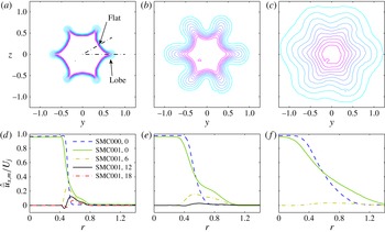
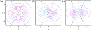
(a–c) Contour plots of mean axial velocity in the serrated jet (SMC001) at selected axial stations; contour levels are equally spaced between 0.1 and
 $0.9U_{j}$
. (d–f) Non-trivial azimuthal Fourier modes (indicated by the numbers in the legend) at these stations. The radial profiles of the round jet (SMC000) at these axial locations are also depicted in (d–f). (a,d)
 $x=0.5$
, (b,e)
 $x=2.0$
, (c,f)
 $x=5.0$
.

3. Experimental data and its analysis
Bridges & Brown (Reference Bridges and Brown2004) performed a systematic parametric study of the effect of nozzle chevrons on single flow jets in the Small Hot Jet Acoustic Rig (SHJAR) at the NASA Glenn Research Center. The jets considered here are from this database; they were operated at acoustic Mach number
 $M_{a}=0.9$
and temperature ratio
 $T_{j}/T_{\infty }=0.84$
(the SP7 set-point of Tanna (Reference Tanna1977)). The Reynolds number was
 $Re_{j}=1.5\times 10^{6}$
. Of the several nozzles that were tested by Bridges & Brown (Reference Bridges and Brown2004), we restrict our study to the round nozzle (code SMC000) and the baseline chevron nozzle (SMC001) (see figure 1). The latter had 6 isosceles chevrons distributed uniformly around the periphery that tapered into the flow at 5° resulting in a radial penetration of 0.985 mm. This nozzle combined the benefit of aft angle low-frequency noise reduction with a low noise penalty at sideline angles and higher frequencies. Both nozzles had a nominal exit diameter of 50.8 mm.
3.1. Velocity measurements and their processing
The three components of jet velocity were measured using stereoscopic particle image velocimetry (PIV) at 12 different cross-stream planes. The set-up of the PIV system has been documented by Opalski, Wernet & Bridges (Reference Opalski, Wernet and Bridges2005). A total of 200 image pairs were recorded at each cross section, and we extracted the ensemble-averaged axial velocity fields,
 $\overline{u}_{x}$
. Figure 2(a–c) depicts these fields for the SMC001 nozzle at representative axial stations. The ensemble-averaged
 $\overline{u}_{r}$
and
 $\overline{u}_{{\it\theta}}$
fields were approximately 100 times smaller in maximum magnitude compared to
 $\overline{u}_{x}$
, and hence were neglected in the stability calculations.
The PSE formulation requires the mean velocity in polar coordinates,
 $\overline{\boldsymbol{u}}(x,r,{\it\theta})$
. The first step to obtain this was to shift the
 $\overline{u}_{x}$
data so that the axis of the polar coordinates matches best with the geometric centre of the velocity profiles (see Gudmundsson & Colonius Reference Gudmundsson and Colonius2011). Subsequently,
 $\overline{u}_{x}$
was transformed from the original Cartesian grid to a polar grid using 2-D cubic-spline interpolation in MATLAB®. After azimuthal Fourier transform of the
 $\overline{u}_{x}$
data, the modes that are not integer multiples of the chevron count (6 for SMC001) were indeed found to be close to zero. The remaining non-trivial azimuthal modes are shown in figure 2(d–f) at the axial stations corresponding to figure 2(a–c). As expected, the azimuthal complexity
 $J$
decreases with downstream distance from the nozzle exit. In fact, at
 $x=5$
, only modes 0 and 6 show significant values. Even at the most upstream station considered in this work (
 $x=0.5$
), the only non-trivial azimuthal modes are 0, 6, 12 and 18. The axisymmetric mode of the mean flow in the SMC000 case is also presented in figure 2(d–f). At all the axial stations depicted, higher radial gradients are displayed by the round jet compared to the
 $m=0$
serrated jet mode.
To facilitate PSE calculations, the SMC001
 $\overline{u}_{x}$
profiles (in the azimuthal Fourier domain) were fitted with smoothing functions consisting of two (possibly truncated) Gaussian curves (see appendix B). The fit coefficients were, in turn, linearly interpolated to the desired axial stations in the PSE calculations to recreate the
 $\overline{u}_{x}$
thereat. The Crocco–Busemann relation along with the ideal gas law (applied to the mean flow quantities) were used to calculate the mean specific volume
 $\overline{{\it\zeta}}$
(which was not available from the experiments).
3.2. Pressure measurements and their processing
Pressure data were acquired on a 78-microphone phased array at SHJAR that was specifically designed to detect instability waves in the hydrodynamic near field of the jet (Suzuki & Colonius Reference Suzuki and Colonius2006). The microphone tips form a cone with a half-angle of 11.3° that intercepts the
 $x=0$
plane at
 $r=0.85$
. Six microphones were uniformly distributed around the azimuth on each of thirteen axial planes spaced
 $0.625D$
apart, starting from
 $x=0.125$
. This allowed the detection of the most energetic azimuthal modes of near-field pressure, viz.
 $m=0$
, 1 and 2.
The microphone signals were simultaneously sampled at 50 kHz for 10 s. This time series is divided into 2976 contiguous segments, each with 168 samples. The consequent frequency resolution in temporal Fourier transform is
 ${\rm\Delta}St=0.05$
. Azimuthal Fourier transform is also applied to this data, so that 2976 realizations of complex pressure fluctuations are obtained in the
 $St{-}m$
domain, each realization having information simultaneously at all axial stations. In each
 $St{-}m$
mode, the pressure amplitude (whose dimensional unit is
 $\text{Pa}~\text{Hz}^{-1/2}$
, but is herein reported in non-dimensional form) is computed as the root mean square of the realizations.
4. LES database
The LES database used in this work was developed to simulate the jet issuing from the SMC001 chevron nozzles at the same operating conditions as in the experiments reported in § 3. The numerical scheme was a hybrid of implicit LES coupled with Spalart–Almaras near-wall RANS modelling. The flow solver, FLUXp, was based on a cell-centred finite-volume discretization for arbitrarily unstructured meshes. However, hexahedral body-fitted meshes with conformed multi-block structured topologies were used to avoid excessive cell skewness around the challenging chevron geometry. The time integrator consisted of a three-step backward Euler implicit scheme for the physical time and a three-stage Runge–Kutta scheme for the pseudo time. The original calculation (Xia et al.
Reference Xia, Tucker and Eastwood2009) was performed on a 12.5 million cell mesh. Following the subsequent success in simulating the SMC006 chevron case on a 20 million cell mesh (Xia & Tucker Reference Xia and Tucker2012), the SMC001 case was also rerun on a mesh having 20 million cells. The simulation time step was
 $5\times 10^{-4}D/U_{j}$
, and it was run for a flow time duration of
 $200D/U_{j}$
beyond the initial transients.
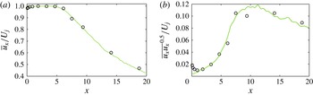
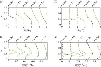
Comparisons of the LES data with the experiments are presented in appendix C. Overall, the statistics are replicated well. However, the LES displays a laminar boundary layer at the nozzle exit that transitions to turbulence by
 $x\approx 0.7$
, whereas the experiments had a turbulent shear layer throughout. The discrepancies with experiment are deemed acceptable given that (a) the LES database is only used to validate the modelling approach, and (b) the base flow for this validation is the mean of the LES data itself.
For the purpose of the present validation, the simulation data was extracted on a structured cylindrical grid having 200 radial grid points in
 $0\leqslant r\leqslant 5$
, with clustering near the lip line. The uniform azimuthal grid had 120 points. The axial domain in
 $0<x<10$
was sampled at 130 planes. In a departure from the experimental data, the mean radial and azimuthal components of velocity of the LES data were found to be non-trivial (about
 $1/10$
th of the mean axial velocity in maximum). This difference from experimental observation may be attributed to the initial laminar state of the LES jet. The mean flow data was processed for PSE calculations using the smoothing procedure described in appendix B.
The LES pressure fluctuation data must be transformed to the frequency domain for comparison with the PSE solution. To obtain statistically significant results, the LES time series (which was sampled at intervals of
 $0.02D/U_{j}$
) was first divided into 75 %-overlapping Hann-windowed segments. For estimating the
 $St=0.25$
mode, each segment length was chosen to be sufficient for resolving
 $1/4$
th of this frequency (i.e. it was
 $16D/U_{j}$
long). Thirty-four such segments were obtained from the available data record, and they were considered independent realizations. Similar considerations yielded 41 and 49 realizations of the
 $St=0.3$
and 0.35 modes, respectively, and so on. Further discussion of the data processing is deferred to § 5.3.
5. Results
5.1. Modal solutions from parallel-flow LST applied to experimental data
The PSE calculations are initiated from the appropriate LST eigensolutions near the nozzle exit. Thus, we start by describing the characteristics of the latter. The base flow for the results presented in this sub-section come from the experimental database discussed in § 3. Converged eigensolutions were found with 800 radial grid points and
 $N=8$
(the degree of azimuthal modal coupling in (2.5)).
Unstable portions of eigenspectra (growth rates
 $-{\it\alpha}^{i}$
versus phase speeds
 $c_{p}={\it\omega}/{\it\alpha}^{r}$
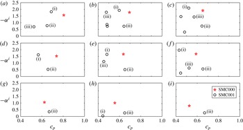
) for the round (SMC000) and serrated (SMC001) jets in
 $St=0.35$
mode, computed from experimental data. (a,d,g)
 $M=0$
, (b,e,h)
 $M=1$
, (c,f,i)
 $M=2$
. (a–c)
 $x=0.5$
, (d–f)
 $x=1.0$
, (g–i)
 $x=2.0$
.

Figure 3 presents the unstable portion of the eigenspectra at three axial stations for the representative
 $St=0.35$
mode. We observe significant differences between the results for the round and serrated jets. The round jet has at most one unstable mode in each
 $St{-}m$
pair, as has been repeatedly shown earlier (e.g. Batchelor & Gill Reference Batchelor and Gill1962). The most striking difference in the serrated jet is the multitude of unstable modes in several of the
 $St{-}M$
pairs shown. At
 $x=0.5$
, there are three unstable modes in
 $M=0$
but five each in
 $M=1$
and 2. On the other hand, at
 $x=2$
only the case of
 $M=1$
has more than one unstable modes. The eigenspectra at
 $x=1$
present an intermediate picture. The
 $M=3$
results are omitted for brevity in this article.
Near the nozzle, the most unstable mode for each
 $M$
in the serrated jet has a slightly higher growth rate but lower phase speed than that in the round jet. At
 $x=1$
(the next axial station for which mean flow data was available), the maximum growth rates of the two jets are more comparable. By
 $x=2$
and beyond, however, the serrated jet has significantly reduced instability compared with the round jet. The phase speeds of unstable modes in the serrated jet exceed those in the round jet at
 $x=2$
.
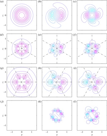
Real parts of pressure eigenfunctions computed at
 $x=1$
in
 $St=0.35$
mode for the round jet SMC000 (a–c) and serrated jet SMC001 (d–l). The dark solid lines are positive contours; light dotted lines are negative ones. Contour levels are equally spaced between
 $\pm 0.95$
of the maximum magnitudes of the respective eigenfunctions. Azimuths of maxima are overlaid for reference. The chevron tips are in the
 $y=0$
plane. (a,d,g,j)
 $M=0$
, (b,e,h,k)
 $M=1$
, (c,f,i,l)
 $M=2$
. With reference to figure 3, where the unstable eigenvalues of the serrated jet are numbered, we present the eigenfunctions of mode (i) (d–f), mode (ii) (g–i), and mode (iii) (j–l).

The rapid modification of the eigenspectrum with axial distance from the nozzle exit reflects the rapidity of the mean flow changes in this region of the serrated jet. Since the LST assumes a parallel flow, one is led to question the physical meaning of the LST results in this zone of rapid change. We choose to initiate the PSE calculations from
 $x=1.0$
. Initiation from further downstream (where the instabilities grow milder) stands to overlook the interesting effects of the serrated mean flow on stability.
The geometrical structure of pressure fluctuations in the most unstable
 $St=0.35$
eigenmodes at
 $x=1$
are shown in figure 4. The presentation is more intuitive in the
 $r-{\it\theta}$
space rather than the coupled azimuthal Fourier domain. The eigenfunctions of the round jet have the expected monopole, dipole and quadrupole character in
 $m=0$
, 1 and 2, respectively. Owing to coupling with higher-order azimuthal Fourier modes, the results for the corresponding azimuthal orders in the serrated jet display greater azimuthal complexity. (Although not shown here, the magnitudes of the pressure eigenfunctions have the 6-fold azimuthal symmetries established in (A 1).) Since the mean flow is axisymmetric away from the lip line, the higher-order coupled
 $m$
-behaviour of the pressure eigenfunctions is strongest only within the shear layer. That is, the
 $m=M$
mode dominates the centreline region as well as the far field.
Next we consider the different instability modes of the serrated jet (only modes (i) to (iii) are depicted). Although modes (i) and (ii) differ in their radial extents and relative azimuthal orientations, they display similar azimuthal complexity. Mode (iii) (and the remaining instabilities that are not shown) have higher azimuthal complexities, and typically display narrower radial support; these suffer rapid damping downstream (see figure 3), and hence will not be discussed in further detail.
The relative azimuthal orientations of modes (i) and (ii) are significant since they are with respect to the lobes in the mean flow. In the mean flow contours presented in figure 2(a), two extremal azimuthal angles are depicted – 0° corresponds to a ‘lobe’ whereas the contours are relatively ‘flat’ around 30°. Of course, this pattern repeats every 60°. The eigenfunctions in mode (i), which are the most unstable at
 $x=1$
, are seen to reach their maxima (in absolute value) at the flats. Conversely, mode (ii) eigenfunctions, which are significantly less unstable, have maxima at the lobes. This is true for all azimuthal orders depicted in figure 4. The analysis in appendix D proposes a tentative explication of the multiple instabilities.
Real parts of pressure eigenfunctions of most unstable
 $St=0.35$
modes computed at
 $x=2$
for the serrated jet (SMC001). The scheme of contour plots follow figure 4. (a)
 $M=0$
, (b)
 $M=1$
, (c)
 $M=2$
.

The most unstable
 $St=0.35$
eigenfunctions calculated at
 $x=2$
are presented in figure 5. The azimuthal orientations of the most unstable modes at
 $x=2$
resembles those of mode (ii) at
 $x=1.0$
. Compared with the latter, the major difference is the increase of radial support of the eigenfunctions, corresponding to the spread of the shear layer. This result justifies the labelling of the unstable eigenmodes at
 $x=2$
in figure 3.
In summary, the most unstable eigenmode near the nozzle, mode (i), displays peaks at the flats of the mean flow contours. However, this eigenmode stabilizes by
 $x\approx 2$
. The other unstable eigenmode with broad radial support, mode (ii), has peaks at the lobes, and has much lower growth rate near the nozzle. However, this mode doesn’t decay very quickly, and in fact becomes the most unstable mode by
 $x=2$
. The other eigenmodes that are unstable near the nozzle have all stabilized by this axial station (see figure 3).
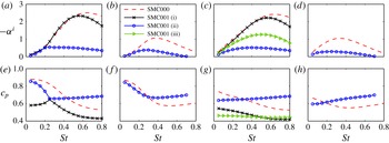
(a–d) Growth rates and (e–h) phase speeds of the unstable modes in the round (SMC000) and serrated (SMC001) jets in
 $M=0$
(a,b,e,f) and
 $M=1$
(c,d,g,h) azimuthal orders and
 $x=1$
(a,c,e,g) and
 $x=2$
(b,d,f,h).

The discussion of the eigenspectra of serrated jets is broadened to include other
 $St$
-modes in figure 6. The
 $St$
-variation of the growth rates and phase speeds of the unstable eigenmodes are shown for
 $M=0$
and 1 at two axial stations. These plots bear out the statements made previously regarding the relative instabilities of the round and serrated jets. In particular, the serrated jet is slightly more unstable near the nozzle (for lower frequencies), but this scenario is inverted by
 $x=2$
. The conclusions regarding the relative phase speeds drawn from the
 $St=0.35$
result are also replicated at all the
 $St{-}M$
modes studied.
5.2. Comparison of PSE solutions with near-field pressure recorded in experiments
The PSE method is now applied to the experimental mean flow data. The PSE formulation forces the solution to approach the most unstable LST mode at each axial station in the downstream march. Since the mode (ii) has been found to be the only unstable mode for
 $x>2$
, we initiate the PSE calculations from the mode (ii) LST solutions computed at
 $x=1$
; the choice of this axial station has been explained above. It is theoretically possible to consider multiple modes in nonlinear PSE (Herbert Reference Herbert1994), but the indeterminacy of their relative initial amplitudes as well as the closure problem in the turbulent flow being considered make this approach unsuitable.
The near-field pressure signature predicted by PSE is compared with the microphone array measurements described in § 3.2. The phased microphone array, having six microphones at each axial station, can resolve Fourier azimuthal modes up to
 $m=2$
; however, we restrict the study to
 $m=0$
and 1 since they are sufficient for clarifying the trends.
The instability waves being modelled here are coherent over large domains. However, the pressure record contains fluctuations over a range of spatial scales. Thus, the two are not directly comparable. Proper orthogonal decomposition is a filtering tool for extracting the energetically-dominant coherent fluctuation modes from turbulent flows. Gudmundsson & Colonius (Reference Gudmundsson and Colonius2011) have described the application of the technique to the round jet’s near-field pressure data sampled on the conical surface formed by the microphone array; the filtered signature is termed ‘cone-POD’ mode herein. These authors demonstrated superior match of the instability waves (predicted using PSE) with the first (most dominant) cone-POD mode rather than the unfiltered pressure signals. The POD filtering is no different for the serrated jet; it is described briefly in appendix E. For reference,
 ${\it\lambda}_{{\it\omega},m}^{(1)}$
and
 $\breve{{\it\psi}}_{{\it\omega},m}^{(1)}$
respectively denote the first cone-POD eigenvalue and corresponding pressure eigenfunction in the Fourier mode pair
 ${\it\omega}{-}m$
.
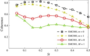
Coherence of the near-field pressure in the round (SMC000) and serrated (SMC001) jets in
 $m=0$
and 1 over a range of
 $St$
-modes. Coherence is measured as the fraction of the pressure fluctuation energy accounted for by the first POD mode, i.e.
 ${\it\lambda}_{{\it\omega},m}^{(1)}/\!\sum _{i}{\it\lambda}_{{\it\omega},m}^{(i)}$
.

The significance of the cone-POD modes is established in figure 7, which displays the relative energy (a fraction between 0 and 1) represented by the first POD mode in the two jets for salient
 $St{-}m$
modes. A fast POD-spectral decay, reflected in a larger value for
 ${\it\lambda}_{{\it\omega},m}^{(1)}/\!\sum _{i}{\it\lambda}_{{\it\omega},m}^{(i)}$
, indicates greater coherence in the data. Conversely, a randomly composed data set will show a flat spectrum, and thus a small value for this fraction. In general, the round jet is more coherent than the serrated one. Thus, the impingement of the nozzle chevrons on the shear layer makes this turbulent jet measurably more ‘complex’. The decrease in coherence at higher frequencies is due to the narrowness of the energetic portion of the corresponding wavepacket (which we discuss later) compared to the microphone spacing and array extent. The minimum in coherence of the serrated jet around
 $St=0.15$
is unexplained at this time. Overall, however, we conclude that the first POD modes represent a substantial portion of the near-field pressure dynamics even in the serrated jet.
The PSE model in (2.4) being linear and homogeneous, neither depends on nor determines the complex amplitude
 $\mathscr{B}$
of the wavepackets (see (2.5)). These are now determined from a least-squares fit with the data (specifically the first pressure POD mode) as
 $$\begin{eqnarray}[\mathscr{B}_{{\it\omega}}^{M}]_{\mathit{Cone}}=\frac{\langle \breve{{\it\psi}}_{{\it\omega},M}^{(1)},\hat{p}_{{\it\omega}}^{M}\rangle _{\mathit{Cone}}}{\Vert \hat{p}_{{\it\omega}}^{M}\Vert _{\mathit{Cone}}^{2}}.\end{eqnarray}$$
We have used the azimuthal sparsity of the microphone array to retain the lowest-order azimuthal mode of the PSE wavepacket in the solution. Also, the inner product and norm are per the definition in (E 1), with the PSE pressure solution
 $\hat{p}$
(defined as in (2.5) but with arbitrary amplitude) extracted at the microphone array.
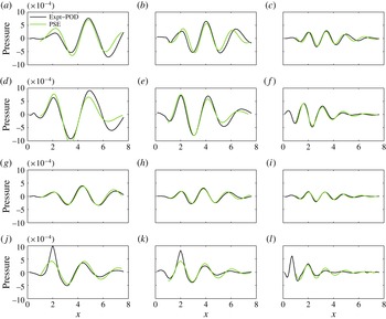
Real part of (Fourier-transformed) pressure along the NASA microphone array for the round (SMC000; a–c, g–i) and serrated (SMC001; d–f, j–l) jets in azimuthal orders (a–f)
 $M=0$
, and (g–l)
 $M=1$
. The first POD mode of the data and the PSE predictions are shown for selected Strouhal numbers. (a,d,g,j)
 $St=0.25$
, (b,e,h,k)
 $St=0.35$
, (c,f,i,l)
 $St=0.5$
.

The real parts of the PSE solution in various
 $St{-}M$
modes are compared with the real parts of the corresponding first POD modes of the data for both round and serrated jets in figure 8. The results from both the experiments and the model are interpolated for presentation. Several differences are observed in the pressure data between the two jets in figure 8 that will be discussed now; the validity of the model will be addressed subsequently. In general, the round jet displays lower levels near the nozzle but retains larger amplitudes further downstream. This effect is linked to the corresponding differences in the streamwise evolution of turbulent kinetic energy in the two jets that have been noted by several researchers (e.g. Bridges & Brown Reference Bridges and Brown2004; Opalski et al.
Reference Opalski, Wernet and Bridges2005; Xia et al.
Reference Xia, Tucker and Eastwood2009). A related observation is the gradual amplification in the round jet vis-à-vis the more abrupt rise in the serrated jet. This is due to the outward jetting effect of the flow through the gaps in between the serrations of the nozzle. An observation of interest is the overall similarity of the phase speeds (proportional to the wavelengths) in the round and serrated jets, although the latter displayed slightly higher phase speeds at
 $x=2$
in figure 6.
Contours of total turbulence amplitude (normalized by
 $c_{\infty }$
) for the (a) round (SMC000) and (b) serrated (SMC001) jets, along with the microphone ring at
 $x=2$
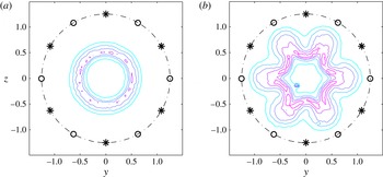
. The circles on the ring denote its six microphones while the stars denote those on an adjacent ring. Five contour levels are equally spaced between 0.04 and 0.2.

An aspect of the pressure evolution curves shown in figure 8 that is an artefact of the geometry of the phased-array measurement system, is the oscillation of amplitudes recorded on alternate axial rings for
 $M=1$
, as evidenced by the localized spikes. Figure 9 shows that the azimuthal position of the microphones relative to the turbulence is different in the two jets. For the serrated jet, all six microphones come equally close to the lobes at
 $x=2$
, so that they yield an overestimate of the pressure fluctuations that would be measured had there been more sensors in between. Conversely, at the previous and next rings, the microphones are located near the troughs of the contours, and thus deliver underestimates. The oscillations are strongest near the nozzle since the lobes of the jet are most pronounced thereat. Actually the oscillations are more pronounced in the original data prior to POD filtering (not shown), and also appear in the unfiltered
 $M=0$
amplitude envelopes.
We now turn to the comparison of prime interest in this work, which is the validation of the PSE predictions for the serrated jet. Considering the
 $St=0.35$
,
 $M=0$
mode, the match between the model and the first POD mode is noteworthy in figure 8. The significantly earlier saturation of the instability waves in the serrated jet (compared to those in the round jet) is faithfully replicated by the model. The phase variations of the wavepacket are also captured well. The match is good in these respects for the
 $St=0.5$
,
 $M=0$
wavepacket too, although minor discrepancies are apparent in the downstream decaying portion. However, the model reproduces the faster decay of the wavepackets, compared to those at
 $St=0.35$
. The model is less successful for the lower frequency of
 $St=0.25$
,
 $M=0$
– a trend that carries over from the round jet model; see discussion below.
Apart from the ring-to-ring oscillations of the POD modes (which our model is not intended to replicate), the agreement is also quite satisfactory for the wavepacket at
 $St=0.35$
,
 $M=1$
. The POD wavepacket at
 $St=0.5$
,
 $M=1$
is dominated by the artificial near-nozzle oscillation described above, which degrades the overall match with the PSE model. The instability wave model is also less accurate at
 $St=0.25$
,
 $M=1$
as in the axisymmetric mode discussed above.
Considering the round jet results, figure 8 demonstrates that the PSE model predictions are generally in good agreement with the first cone-POD mode. The model predictions at
 $St=0.25$
, particularly in
 $m=0$
, are less accurate; this trend continues to lower frequencies. Gudmundsson & Colonius (Reference Gudmundsson and Colonius2011) reported similar deficiencies of the PSE model for the round jet instabilities, and Baqui et al. (Reference Baqui, Agarwal, Cavalieri and Sinayoko2013) observed the same behaviour for instability waves derived from linearized Euler equations. The discrepancy is likely due to nonlinear effects on these modes, as well as a possible inadmissibility of the mildly non-parallel assumption for these long-wavelength wavepackets (Gudmundsson & Colonius Reference Gudmundsson and Colonius2011; Baqui et al.
Reference Baqui, Agarwal, Cavalieri and Sinayoko2013; Sinha et al.
Reference Sinha, Rodríguez, Brès and Colonius2014).
To quantify the foregoing comparisons, we propose the following ‘alignment’ metric
 $$\begin{eqnarray}[\mathbb{A}_{{\it\omega}}^{M}]_{\mathit{Cone}}=\frac{|\langle \breve{{\it\psi}}_{{\it\omega},M}^{(1)},\hat{p}_{{\it\omega}}^{M}\rangle _{\mathit{Cone}}|}{\Vert \breve{{\it\psi}}_{{\it\omega},M}^{(1)}\Vert _{\mathit{Cone}}\Vert \hat{p}_{{\it\omega}}^{M}\Vert _{\mathit{Cone}}},\end{eqnarray}$$
where the notation carries over from (5.1). The intent is to determine, for a given
 ${\it\omega}{-}M$
pair, the degree of closeness (in the vector alignment sense) of the fundamental Fourier azimuthal mode (
 $m=M$
) in the PSE pressure wavepacket with the corresponding first cone-POD mode of the experimental pressure data. The result is a number between 0 and 1, with 1 indicating perfect prediction and 0 representing failure of the model. An analogous metric was considered by Sinha et al. (Reference Sinha, Rodríguez, Brès and Colonius2014).
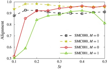
Alignment of the near-hydrodynamic pressure of the PSE wavepackets with the first POD modes of the corresponding experimental data for the round (SMC000) and serrated (SMC001) jets in azimuthal orders
 $M=0$
and 1 for various
 $St$
modes.

The alignment metrics are presented in figure 10 for a range of
 $St$
-modes, computed for both the round and serrated jets. A high degree of alignment (
 ${>}0.84$
) is verified in the serrated jet for
 $0.2\leqslant St\leqslant 0.45$
, both for
 $M=0$
and 1. This reinforces the qualitative agreement of the model demonstrated in figure 8. Also, the model predictions display similar accuracy in the serrated jet as in the round jets. However, the relative accuracies in the
 $M=0$
and 1 are inverted in the two jets. This is due to the artificial ring-to-ring oscillation that is prominent in the
 $M=1$
POD modes of the serrated jet. This is most apparent in the
 $St=0.5$
case, which has been discussed in the context of figure 8. The drastic degradation of accuracy of the serrated jet model for
 $St<0.2$
may be explained thus. The intense mixing generated by the chevrons results in a quick growth of the shear layer. Compared to the round jet, this further belies the mildly non-parallel base flow assumption for long-wavelength low-frequency wavepackets in serrated jets.
Lastly, we note that the alignment metric for the low-frequency modes in the round jet is not as low as the results in figure 8 may have led one to expect. Actually, for a fairer quantitative comparison across frequencies, the axial domain of the inner product should be modified to include a certain number of wavelengths for each modal frequency being studied. However, the limited axial extent of the microphone array as well as its axial resolution disallow this exercise.
5.3. Comparison of PSE solutions with pressure extracted from the LES database
We now investigate the degree to which the PSE wavepackets describe the flow fluctuations within the turbulent shear layer. Time-resolved experimental data are unavailable for this purpose, so we turn to the LES database of the serrated jet with its space- and time-resolved flow information. It has been remarked in § 4 that the near-nozzle region of the flow observed in experiments is not replicated completely by the LES database. This affects the LST eigenmodes that constitute the initial condition of the PSE, as well as the PSE calculations themselves.
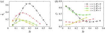
(a) Growth rates and (b) phase speeds of unstable LST eigenmodes of the serrated (SMC001) LES jet evaluated at
 $x=1$
and 2.

The LST eigenvalues computed from the LES mean flow field at
 $x=1$
and 2 are presented in figure 11. The most prominent difference in the results is the presence of only one unstable eigenmode at each
 $St{-}M$
condition in the case of the LES, instead of the multitude found with experimental mean flow. Moreover, although the trends with
 $St$
,
 $M$
and
 $x$
are similar to the results for instability mode (ii) obtained with experimental data (see figure 6), the growth rates are diminished. Both these discrepancies may be attributed to the increased thickness of the shear layer in the LES jet. The differences in the phase speeds between the two cases do not follow any distinct pattern.
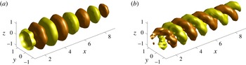
Representative positive and negative isosurfaces of the real part of pressure in the PSE solution for the serrated (SMC001) LES jet for
 $St=0.3$
corresponding to azimuthal orders (a)
 $M=0$
, and (b)
 $M=1$
. The chevron tips are in the
 $y=0$
plane.

A depiction of the wavepacket nature of the PSE solution is presented in figure 12. This clearly shows the serrated nature of the near-nozzle PSE solution that couples higher-order azimuthal modes. The solution tends to lose the serrated character further downstream, and resembles those computed in round jets.
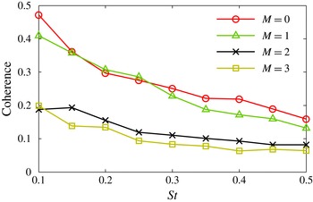
Coherence of the pressure field in the serrated (SMC001) LES jet, measured as the fraction of the pressure fluctuation energy accounted for by the first POD mode, i.e.
 ${\it\Lambda}_{{\it\omega}}^{M,(1)}/\sum _{i}{\it\Lambda}_{{\it\omega}}^{M,(i)}$
.

The wavepacket structure embedded in turbulence is clearest in the pressure fluctuation field (Sinha et al.
Reference Sinha, Rodríguez, Brès and Colonius2014). To identify the wavepackets, ‘volumetric’ POD filtering is performed on the pressure data extracted on the structured cylindrical grid mentioned in § 4 using the method described in appendix F. For reference,
 ${\it\Lambda}_{{\it\omega}}^{M,(1)}$
and
 $\hat{{\it\phi}}_{{\it\omega}}^{M,(1)}$
respectively denote the first volume-POD eigenvalue and corresponding pressure eigenfunction in the frequency
 ${\it\omega}$
and azimuthal order
 $M$
.
The coherence of this data, as measured by
 ${\it\Lambda}_{{\it\omega}}^{M,(1)}/\sum _{i}{\it\Lambda}_{{\it\omega}}^{M,(i)}$
, is shown in figure 13. The
 $M=0$
and 1 fluctuations are more ordered than those in higher azimuthal orders, an observation that carries over from supersonic round jets (Sinha et al.
Reference Sinha, Rodríguez, Brès and Colonius2014). There is also a monotonic decrease of coherence with frequency – a phenomenon that was not observed in the supersonic round jets. The impingement of the nozzle serrations on the jet shear layer appears to be selectively reducing the organization of the turbulent structures at higher frequencies.
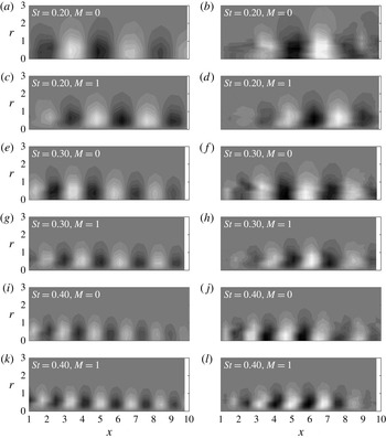
Real parts of least-order azimuthal modes of pressure in PSE solution (a,c,e,g,i,k) compared with corresponding components of first POD mode from LES database (b,d,f,h,j,l) for
 $St=0.2$
, 0.3 and 0.4 and azimuthal orders
 $M=0$
and 1 as labelled. Contour levels are identical between each pair of (left and right panels), but not across rows.

As in the case of near-field pressure comparisons in § 5.2, the complex amplitudes of the PSE modes are fitted to the LES pressure data as follows
 $$\begin{eqnarray}[\mathscr{B}_{{\it\omega}}^{M}]_{\mathit{Vol}}=\frac{\langle \hat{{\it\phi}}_{{\it\omega}}^{M,(1)},\hat{p}_{{\it\omega}}^{M}\rangle _{\mathit{Vol}}}{\Vert \hat{p}_{{\it\omega}}^{M}\Vert _{\mathit{Vol}}^{2}}.\end{eqnarray}$$
Note that all the coupled azimuthal modes of the solution and data are considered in the above. The inner product and norm are per the definition in (F 1).
The real parts of the lowest-order azimuthal modes (i.e.
 $m=0$
in case of
 $M=0$
and
 $m=1$
in case of
 $M=1$
) of pressure in the PSE solution are depicted in figure 14 alongside the corresponding first POD modes from the LES data. The wavelength (and hence the phase speeds) of the predicted wavepackets are seen to resemble those in the data in all cases. The amplitude of the wavepackets also display a fair match, although the decaying zones are typically under predicted. This behaviour of stability-based models has been discussed by Rodríguez et al. (Reference Rodríguez, Cavalieri, Colonius and Jordan2015). The
 $m=1$
mode comparisons are better than those for
 $m=0$
, an observation that carries over from PSE models of round jets (Sinha et al.
Reference Sinha, Rodríguez, Brès and Colonius2014).
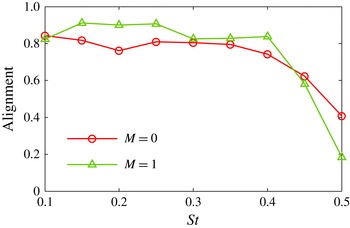
Alignment of the pressure component of the PSE wavepackets with the first POD modes of the corresponding LES data for the serrated (SMC001) jets in azimuthal orders
 $M=0$
and 1 for various
 $St$
modes.

The following ‘alignment’ metric quantifies the comparison between the PSE pressure solution and the corresponding first POD mode of LES (see also (5.2))
 $$\begin{eqnarray}[\mathbb{A}_{{\it\omega}}^{M}]_{\mathit{Vol}}:=\frac{|\langle \hat{p}_{{\it\omega}}^{M},\hat{{\it\phi}}_{{\it\omega}}^{M,(1)}\rangle _{\mathit{Vol}}|}{\Vert \hat{p}_{{\it\omega}}^{M}\Vert _{\mathit{Vol}}\Vert \hat{{\it\phi}}_{{\it\omega}}^{M,(1)}\Vert _{\mathit{Vol}}}.\end{eqnarray}$$
The calculated values of the alignment metric are presented in figure 15 for two azimuthal orders over a range of frequencies. Overall, we demonstrate a high degree of alignment, further justifying the use of PSE for predicting wavepackets that are actually present in the turbulent serrated jet. The alignment is generally better in case of
 $M=1$
, as also noted from figure 14. The apparent inversion of this trend in the near-field pressure results of § 5.2 has been explained as an artefact of the microphone array design.
The drastic degradation of alignment of the PSE solutions for frequencies beyond
 $St=0.4$
can be explained with reference to the LST results at the initial axial station. Figure 11 shows that these modes are close to stable already, and in fact they are stable at the next axial step. Thus, these wavepackets start to decay very close to the nozzle exit, and the PSE method is unable to replicate the decay behaviour well. In the LST solution, the
 $M=1$
mode stabilizes at a lower frequency compared to the
 $M=0$
mode (see figure 11) – a fact that explains the corresponding poorer alignment of the
 $M=1$
PSE solutions for
 $St>0.4$
in figure 15.
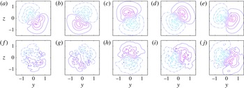
Real parts of pressure in PSE solution (a–e) and first POD mode of LES data (f–j) at various cross sections in the
 $St=0.3$
,
 $M=1$
case. Contour levels are equally spaced between
 $\pm 0.9$
of the maximum value found in the entire domain. (a,f)
 $x=2.2$
, (b,g)
 $x=2.6$
, (c,h)
 $x=3.4$
, (d,i)
 $x=3.7$
, (e,j)
 $x=4.0$
.

A detailed picture of the azimuthal variation of a wavepacket is presented in figure 16. The PSE pressure solution for the
 $St=0.3$
,
 $M=1$
case is scaled by the complex amplitude
 $\mathscr{B}$
found in (5.3), and its real part is compared with the corresponding first pressure POD mode of the LES data at various cross sections. The POD modes retain some uncertainty, which could have been reduced if a longer time record were available. We note significant similarities in the rotational phase variation and the radial shape. The quantitative comparison of these cross-sectional shapes is a part of the alignment metric of (5.4).
6. Summary and conclusions
We solve the mildly non-parallel linear PSE for a natural turbulent jet issuing from a nozzle with serrations (chevrons) distributed uniformly around the periphery. The time-averaged flow field, which displays corresponding serrations in its contour plots, is used as the base flow for the stability calculations. The streamwise evolution of linear perturbations of this base flow is intended to model the large-scale coherent structures in the serrated jet. The PSE calculations are initiated near the nozzle from eigensolutions of the classical parallel-flow linear stability theory (LST). In the past, this approach has delivered a good match with experimental and numerical datasets of turbulent round jets.
Unlike the 2-D (i.e.
 $x{-}r$
) PSE of round jets wherein the Fourier azimuthal modes (in addition to the frequency modes) are decoupled, the non-axisymmetry of the serrated jets leads to a 3-D (i.e.
 $x{-}r{-}{\it\theta}$
) PSE problem. However, we show here that due to the regular arrangement of the serrations (say
 $L$
in number), the corresponding serrations of the mean flow field have an
 $L$
-fold rotational symmetry. An additional mirror symmetry exists in the mean flow since the individual serrations are typically mirrored about a centre plane. These symmetries are exploited here to derive a series of equivalent 2-D PSE problems, each with sparse coupling in the Fourier azimuthal domain. Compared to the 3-D problem, the individual 2-D problems have reduced dimensionality by a factor of
 $L$
or
 $L/2$
, depending on the particular member of the series considered. Aside from the computational efficiency, an advantage of the coupled 2-D PSE formulation is the clarification it provides regarding the geometrical structure of the solutions. The LST problem, which is solved at the near-nozzle cross section of the jet to initiate the PSE calculations, also has corresponding simplifications.
We investigate the nominal (SMC001) serrated jet and the corresponding (SMC000) round jet that were operated cold at Mach 0.9 in experiments at NASA by Bridges & Brown (Reference Bridges and Brown2004). Using their ensemble-averaged velocity fields as base flows, the LST reveals multiple unstable eigenmodes in the serrated jet at cross sections very near the nozzle; round jets have at most one unstable mode at any cross section. These new instability modes arise due to the azimuthal shear in the mean flow field. Alternatively, they can be viewed as consequences of the Fourier azimuthal coupling of the 1-D eigenproblems. Very near the nozzle exit (i.e. at
 $x=0.5D$
), the most unstable modes in the serrated jet display slightly higher growth rates compared to the corresponding round jet modes. However, the growth rates of the serrated jet modes decrease dramatically by
 $x=2D$
, and are much less unstable than their round jet counterparts thereat. In fact, beyond
 $x=2D$
, the most unstable eigenmode observed near the nozzle stabilizes and a less unstable mode prevails. The phase speeds of the most unstable serrated jet modes start out as lower than the corresponding round jet modes near the nozzle, but become approximately similar further downstream.
The recent literature has provided a method to educe wavepackets from a natural turbulent flow by filtering its near-field hydrodynamic pressure data with POD. The PSE solutions are compared with the wavepackets thus extracted from the NASA experiments on the serrated jet. A reasonable match is demonstrated between the two over the Strouhal number range of
 $0.2\leqslant St\leqslant 0.45$
. The failure at higher frequencies is arguably attributable to the data, but that at lower frequencies possibly implicates nonlinear effects. The degree of matching in serrated jets is quite similar to that in round jets, even though the POD spectral decay is considerably slower in the former case (which indicates its lower coherence). The data (which the PSE model replicates) reveals that the near-field hydrodynamic pressure fluctuations are more energetic in the round jet compared to the serrated jet.
To validate the detailed structure of the wavepackets predicted by our PSE model within the shear layer of the jet, we utilize an LES database that simulates the same serrated jet. The LES jet has a transitional nature up to
 $x\approx 0.7$
, so that the near-nozzle region of the experimental jet is not replicated exactly. In particular, at most one unstable mode is obtained in the LST of this jet at all relevant cross sections. The shapes of the PSE pressure solution are compared visually and quantitatively with the POD-filtered pressure modes of the LES data over a cylindrical domain extending from
 $x=1$
to
 $x=10$
. Encouraging agreement is obtained across the
 $St$
-range mentioned above.
We conclude that the PSE model captures the major features of the coherent wavepackets observed in the hydrodynamic pressure field of the turbulent serrated jet.
Acknowledgements
We thank Dr J. Bridges and C. Brown of NASA Glenn Research Center for providing the experimental database. We are also grateful to Drs A. Samanta and D. Rodríguez for contributing to the development of the PSE code for the round jet. Discussions with Dr A. Uzun were useful in the course of this work. A.S. and T.C. acknowledge support from the Office of Naval Research under contract N0014-11-1-0753 with Dr B. Henderson as technical monitor. A.S. is also grateful for support from the Industrial Research and Consultancy Center of Indian Institute of Technology Bombay, via the seed grant program. H.X. acknowledges the HPC time and file storage on the Hydra system of Loughborough University.
Appendix A. Properties of the stability solution
The rotational and mirror symmetries of the mean flow field delineated in § 2 result in the following properties of the linear PSE solutions.
Property 1.
 $L$
-fold rotational symmetry
 $$\begin{eqnarray}\hat{\boldsymbol{q}}_{{\it\omega}}^{M}(x,r,{\it\theta}+2{\rm\pi}k/L)=\text{e}^{\text{i}2{\rm\pi}kM/L}\hat{\boldsymbol{q}}_{{\it\omega}}^{M}(x,r,{\it\theta}),\quad k\in \mathbb{Z}.\end{eqnarray}$$
Property 2. Mirror symmetry
 $$\begin{eqnarray}{\it\alpha}_{{\it\omega}}^{-M}={\it\alpha}_{{\it\omega}}^{M},\end{eqnarray}$$
 $$\begin{eqnarray}\tilde{q}_{{\it\omega},-m}=\tilde{q}_{{\it\omega},m},\quad \tilde{q}\in \{\tilde{u}_{x},\tilde{u}_{r},\tilde{p},\tilde{{\it\zeta}}\};\quad (\tilde{u}_{{\it\theta}})_{{\it\omega},-m}=-(\tilde{u}_{{\it\theta}})_{{\it\omega},m},\end{eqnarray}$$
 $$\begin{eqnarray}\hat{q}_{{\it\omega}}^{-M}(\cdot ,{\it\theta})=\hat{q}_{{\it\omega}}^{M}(\cdot ,-{\it\theta}),\quad \hat{q}\in \{\hat{u}_{x},\hat{u}_{r},\hat{p},\hat{{\it\zeta}}\};\quad (\hat{u}_{{\it\theta}})_{{\it\omega}}^{-M}(\cdot ,{\it\theta})=-(\hat{u}_{{\it\theta}})_{{\it\omega}}^{M}(\cdot ,-{\it\theta}).\end{eqnarray}$$
As a corollary of (A 2d,e
), we only need to solve for azimuthal orders in the range
 $0\leqslant M\leqslant L/2$
. Moreover, (A 2b,c
) indicates that only
 $N+1$
out of the
 $2N+1$
coupled azimuthal modes in
 $\tilde{\boldsymbol{Q}}^{0}$
are independent, and that
 $(\tilde{u}_{{\it\theta}})_{{\it\omega},0}\equiv 0$
. Finally, for the Nyquist azimuthal order
 $\tilde{\boldsymbol{Q}}^{L/2}$
, only half of the coupled modes are independent. These symmetries further reduce the stability problem dimensionality in the respective azimuthal orders.
Appendix B. Mean flow field fitting functions
The following are the fitting functions for the mean flow variables (in the Fourier azimuthal domain), chosen after studying the data (e.g. figure 2 b).
 $$\begin{eqnarray}\displaystyle & \displaystyle (\check{\overline{u}}_{x})_{m=0}=\left\{\begin{array}{@{}ll@{}}U_{x0}, & r\leqslant r_{x0},\\ U_{x0}[a_{x0}\text{e}^{-(r-r_{x0})^{2}/{\it\delta}_{x01}^{2}}+(1-a_{x0})\text{e}^{-(r-r_{x0})^{2}/{\it\delta}_{x02}^{2}}], & r>r_{x0}.\end{array}\right. & \displaystyle\end{eqnarray}$$
 $$\begin{eqnarray}\displaystyle & \displaystyle (\check{\overline{u}}_{x})_{m>0}=(U_{xm1}\text{e}^{-(r-r_{xm1})^{2}/{\it\delta}_{xm1}^{2}}+U_{xm2}\text{e}^{-(r-r_{xm2})^{2}/{\it\delta}_{xm2}^{2}}){\it\sigma}(r). & \displaystyle\end{eqnarray}$$
 $$\begin{eqnarray}\displaystyle & \displaystyle (\check{\overline{u}}_{r})_{m=0}=\frac{U_{r0}}{1+\text{e}^{-(r-r_{r01})/{\it\delta}_{r01}}}\left(\frac{a_{r0}}{1+\text{e}^{(r-r_{r02})/{\it\delta}_{r02}}}-1\right)\text{e}^{-r/{\it\delta}_{r03}}{\it\sigma}(r), & \displaystyle\end{eqnarray}$$
 $$\begin{eqnarray}\displaystyle & \displaystyle (\check{\overline{u}}_{r})_{m>0}={\it\sigma}(r)U_{rm}\left\{\begin{array}{@{}ll@{}}\text{e}^{-(r-r_{rm})^{2}/{\it\delta}_{rm1}^{2}}, & r<r_{rm},\\ \text{e}^{-(r-r_{rm})^{2}/{\it\delta}_{rm2}^{2}}, & r\geqslant r_{rm}.\end{array}\right. & \displaystyle\end{eqnarray}$$
 $$\begin{eqnarray}\displaystyle & \displaystyle (\check{\overline{u}}_{{\it\theta}})_{m=0}=0. & \displaystyle\end{eqnarray}$$
 $$\begin{eqnarray}\displaystyle & \displaystyle (\check{\overline{u}}_{{\it\theta}})_{m>0}=(U_{{\it\theta}m1}\text{e}^{-(r-r_{{\it\theta}m1})^{2}/{\it\delta}_{{\it\theta}m1}^{2}}+U_{{\it\theta}m2}\text{e}^{-(r-r_{{\it\theta}m2})^{2}/{\it\delta}_{{\it\theta}m2}^{2}}){\it\sigma}(r). & \displaystyle\end{eqnarray}$$
 $$\begin{eqnarray}\displaystyle & \displaystyle \check{\overline{{\it\zeta}}}_{m=0}=\left\{\begin{array}{@{}ll@{}}1+{\it\zeta}_{01}, & r\leqslant r_{{\it\zeta}01},\\ 1+{\it\zeta}_{01}\text{e}^{-(r-r_{{\it\zeta}01})^{2}/{\it\delta}_{{\it\zeta}01}^{2}}+{\it\zeta}_{02}\text{e}^{-(r-r_{{\it\zeta}02})^{2}/{\it\delta}_{{\it\zeta}02}^{2}}, & r>r_{{\it\zeta}01}.\end{array}\right. & \displaystyle\end{eqnarray}$$
 $$\begin{eqnarray}\displaystyle & \displaystyle \check{\overline{{\it\zeta}}}_{m>0}=({\it\zeta}_{m1}\text{e}^{-(r-r_{{\it\zeta}m1})^{2}/{\it\delta}_{{\it\zeta}m1}^{2}}+{\it\zeta}_{m2}\text{e}^{-(r-r_{{\it\zeta}m2})^{2}/{\it\delta}_{{\it\zeta}m2}^{2}}){\it\sigma}(r). & \displaystyle\end{eqnarray}$$
 $$\begin{eqnarray}\displaystyle & \displaystyle {\it\sigma}(r)=2/(1+\text{e}^{-20r})-1. & \displaystyle\end{eqnarray}$$
The sigmoid function
 ${\it\sigma}(r)$
is designed to ensure vanishing values at the centreline for specific quantities. All the coefficients are functions of
 $x$
, and are obtained by least-squares fit from data.
Appendix C. LES database validation results
Figures 17 and 18 present the comparison of the time-averaged LES data against the NASA PIV data (described in § 3.1). The centreline velocity and the normal Reynolds stress component are matched well. The radial profiles of these quantities also show significant similarity. However, the LES predicts a somewhat thicker shear layer in the chevron tip plane, especially near the nozzle exit. Xia & Tucker (Reference Xia and Tucker2012) demonstrated favourable agreement of the far-field sound predictions (using a Ffowcs-Williams Hawkings solver) with measured values for the SMC006 nozzle case computed using the same numerical set-up.
(a) Mean axial velocity and (b) its standard deviation along the centreline from LES (curves) compared with experimental data (symbols).

Mean axial velocity (a,b) and its standard deviation (c,d) from LES (solid) compared with experimental data (dotted). The profiles for the root and tip planes of the chevrons are shown in (a,c) and (b,d), respectively.

Appendix D. Analysis of the multiple LST eigensolutions
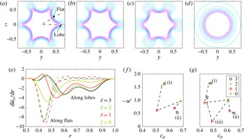
Figure 19 presents the results of an exercise undertaken to seek the origin of the two instability modes in the serrated jet – modes (i) and (ii) – described in § 5.1. The azimuthal complexity of the mean flow profile is identified by
 $J$
(see § 2), and it proves interesting to examine the eigenspectra resulting from separate computations where we retain successively fewer azimuthal modes in the mean flow at
 $x=1$
. The mean axial velocity contours are depicted in figure 19(a–d), and their radial derivatives along the two extremal azimuths (viz. flat and lobe) are presented in figure 19(e). The lobes become successively broader as
 $J$
is decreased from 3 to 1. However, the magnitude of the radial gradient at the lobe actually increases with decreasing
 $J$
. The flats, on the other hand, remain substantially unchanged for
 $1\leqslant J\leqslant 3$
.
(a–d) Contour plots of mean axial velocity in the serrated jet at
 $x=1.0$
for decreasing azimuthal complexity,
 $J$
(from
 $J=3$
in (a) to
 $J=0$
in (d)); contour levels are equally spaced between 0.1 and
 $0.9U_{j}$
. (e) Radial derivative of mean axial velocity for varying
 $J$
at the two extremal azimuthal angles shown in (a). (f,g) Effect of
 $J$
(indicated in legend) on the eigenspectra in
 $M=0$
and 1 modes for
 $St=0.35$
.

Figure 19(f,g) shows the effect of these mean flow modifications on modes (i) and (ii) in
 $M=0$
and 1 at
 $St=0.35$
. The growth rate in mode (i), which peaks at the flats, reduces successively. Conversely, the growth rate in mode (ii), which peaks at the lobes, is enhanced as
 $J$
is decreased. If we simplistically consider round jets consisting of either the flat or lobe profiles, and modes (i) and (ii) to be dictated solely by these respective profiles, then the modification of the mean flow gradients indicated above serve to explain the trends in these growth rates. We conclude that mode (i) is primarily associated with the maximum radial shear occurring at the flats of the mean flow profile (where it peaks in figure 4), and hence has the highest growth rate. Mode (ii), on the other hand, is associated with the second (much weaker) extremal of radial shear at the lobes, and hence displays lower growth rates. The other instability modes display higher azimuthal complexity, and are not covered by this explanation. Note the considerable reduction in both the number and growth rates of these other unstable modes as
 $J$
is decreased.
Appendix E. Cone-POD modes of the jet hydrodynamic near field
As described in § 3.2, the pressure time series recorded on the near-field phased microphone array encasing the jet is divided into segments that are considered independent realizations, and each of these are Fourier transformed in time and azimuth. Let us denote the consequent signal in the
 $k$
th segment at ring axial location
 $x$
, frequency
 ${\it\omega}$
and Fourier azimuthal mode
 $m$
as
 $\breve{\mathscr{P}}_{{\it\omega},m}^{[k]}(x)$
, the radial coordinate being redundant on the conical surface of the array. The azimuthal resolution of the array is not fine enough to evince the coupling due to the lobed azimuthal stochastic structure of the flow; thus the different
 $m$
-modes are considered independent. The inner product for the cone-POD is defined for two realizations
 $\breve{\mathscr{P}}_{{\it\omega},m}^{[i]}$
and
 $\breve{\mathscr{P}}_{{\it\omega},m}^{[j]}$
as
 $$\begin{eqnarray}\langle \breve{\mathscr{P}}_{{\it\omega},m}^{[i]},\breve{\mathscr{P}}_{{\it\omega},m}^{[j]}\rangle _{\mathit{Cone}}=\int \{\breve{\mathscr{P}}_{{\it\omega},m}^{[j]}(x)\}^{\dagger }\breve{\mathscr{P}}_{{\it\omega},m}^{[i]}(x)\,\text{d}x,\end{eqnarray}$$
where
 $(\cdot )^{\dagger }$
denotes complex conjugation, and the integration is over the axial domain of measurement. With this, the integral eigenvalue (POD) problem is (Lumley Reference Lumley, Yaglom and Tatarsky1967)
 $$\begin{eqnarray}\int E[\breve{\mathscr{P}}_{{\it\omega},m}^{[k]}(x_{1})\{\breve{\mathscr{P}}_{{\it\omega},m}^{[k]}(x_{2})\}^{\dagger }]\breve{{\it\psi}}_{{\it\omega},m}(x_{2})\,\text{d}x_{2}={\it\lambda}_{{\it\omega},m}\breve{{\it\psi}}_{{\it\omega},m}(x_{1}),\end{eqnarray}$$
where
 $E(\cdot )$
denotes the expectation over the different realizations, so that the kernel is the 2-point cross-correlation tensor. The eigenvalues
 ${\it\lambda}$
are non-negative, and the eigenfunction
 $\breve{{\it\psi}}$
corresponding to the largest
 ${\it\lambda}$
is the most energetic coherent structure in the data per POD theory. The normalization of the
 $n$
th POD eigenfunction is such that
 $\Vert \breve{{\it\psi}}_{{\it\omega},m}^{(n)}\Vert _{\mathit{Cone}}={\it\lambda}_{{\it\omega},m}^{(n)}$
, where
 $\Vert \cdot \Vert _{\mathit{Cone}}$
is the norm induced by the inner product in (E 1).
Appendix F. Volume-POD modes of the serrated jet
The complex pressure at frequency
 ${\it\omega}$
is denoted
 $\hat{P}_{{\it\omega}}(x,r,{\it\theta})$
. As explained in § 4, we obtain sufficient realizations of this from the LES data, the
 $k$
th being denoted
 $\hat{P}_{{\it\omega}}^{[k]}$
. The inner product for the volume-POD is defined for two such fields
 $\hat{P}_{{\it\omega}}^{[i]}$
and
 $\hat{P}_{{\it\omega}}^{[j]}$
as
 $$\begin{eqnarray}\langle \hat{P}_{{\it\omega}}^{[i]},\hat{P}_{{\it\omega}}^{[j]}\rangle _{\mathit{Vol}}=\int _{-{\rm\pi}}^{{\rm\pi}}\int _{0}^{\infty }\int _{X_{1}}^{X_{2}}\{\hat{P}_{{\it\omega}}^{[j]}(x,r,{\it\theta})\}^{\dagger }\hat{P}_{{\it\omega}}^{[i]}(x,r,{\it\theta})r\,\text{d}x\,\text{d}r\,\text{d}{\it\theta}.\end{eqnarray}$$
Here
 $X_{1}$
and
 $X_{2}$
are respectively the upstream and downstream extents of the data.
As in appendix E, the consequent POD problem is
 $$\begin{eqnarray}\iiint r_{1}^{1/2}E[\hat{P}_{{\it\omega}}^{[k]}(\boldsymbol{x}_{1})\{\hat{P}_{{\it\omega}}^{[k]}(\boldsymbol{x}_{2})\}^{\dagger }]r_{2}^{1/2}r_{2}^{1/2}\hat{{\it\phi}}_{{\it\omega}}(\boldsymbol{x}_{2})\,\text{d}\boldsymbol{x}_{2}={\it\Lambda}_{{\it\omega}}r_{1}^{1/2}\hat{{\it\phi}}_{{\it\omega}}(x_{1},r_{1},{\it\theta}_{1}).\end{eqnarray}$$
The integration limits are omitted for notational convenience. The
 $r^{1/2}$
weightings are introduced to make the problem Hermitian (Baker Reference Baker1977).
The serrated flow geometry has
 $L$
symmetric lobes. Thus, we expect that the cross correlation will be the same if the reference angle is shifted by
 $2{\rm\pi}k/L$
as long as the angular difference between the two correlated quantities is maintained. This symmetry is used to ‘augment’ the data ensemble size, in a manner analogous to POD in the presence of a homogeneous direction (Sirovich Reference Sirovich1987). With the usual definition of azimuthal Fourier transform, and introducing the notation
 $\boldsymbol{y}=(x,r)$
, this results in the simplified kernel
 $$\begin{eqnarray}\displaystyle E[\hat{P}_{{\it\omega}}^{[k]}(\boldsymbol{y}_{1},{\it\theta}+{\it\vartheta})\{\hat{P}_{{\it\omega}}^{[k]}(\boldsymbol{y}_{2},{\it\theta})\}^{\dagger }]=\mathop{\sum }_{m,l=-\infty }^{\infty }E[\breve{P}_{{\it\omega},m}^{[k]}(\boldsymbol{y}_{1})\{\breve{P}_{{\it\omega},m-lL}^{[k]}(\boldsymbol{y}_{2})\}^{\dagger }]\text{e}^{\text{i}(m{\it\vartheta}+lL{\it\theta})}. & & \displaystyle\end{eqnarray}$$
Substituting this in (F 2) and applying azimuthal Fourier transform to the result yields
 $$\begin{eqnarray}\displaystyle \mathop{\sum }_{l=-C}^{C}\iint r_{1}^{1/2}E[\breve{P}_{{\it\omega},m}^{[k]}(\boldsymbol{y}_{1})\{\breve{P}_{{\it\omega},m-lL}^{[k]}(\boldsymbol{y}_{2})\}^{\dagger }]r_{2}\breve{{\it\phi}}_{{\it\omega},m-lL}(\boldsymbol{y}_{2})\,\text{d}\boldsymbol{y}_{2}={\it\Lambda}_{{\it\omega},m}r_{1}^{1/2}\breve{{\it\phi}}_{{\it\omega},m}(\boldsymbol{y}_{1}). & & \displaystyle\end{eqnarray}$$
This represents the reduced POD problem in the presence of the serrated mean flow. The restriction of the summation to
 $\pm C$
reflects the limit of the azimuthal grid resolution of the data, or the vanishing of coupling across a large
 $m$
-range. As an aside, note that for the round jet
 $L\rightarrow \infty$
, so that
 $l$
can only be zero, and we retrieve the fully decoupled set of POD problems, as expected.
The azimuthal coupling exhibited by (F 4) is similar to the PSE problem in § 2. Invoking analogous arguments and using the definition of
 $M$
, we only need to solve for the sets
 $M\in [0,\lceil (L-1)/2\rceil ]$
, the corresponding eigensolutions being denoted by
 ${\it\Lambda}_{{\it\omega}}^{M}$
,
 $\hat{{\it\phi}}_{{\it\omega}}^{M}(\boldsymbol{x})$
. Owing to the mirror symmetry of the serrations, the
 $+m$
and
 $-m$
will have the same statistics, which is to be used to augment the expectation operation in the computation of the kernel (Sirovich Reference Sirovich1987). In the actual implementation, the equivalent snapshot method is used (Sirovich Reference Sirovich1987; Sinha et al.
Reference Sinha, Rodríguez, Brès and Colonius2014).