1. Introduction

Water is found in polycrystalline ice at temperatures close to 0°C within the grains in internal melt-figures and inside bubbles, in the grain boundaries in the form of lenses, and along the lines where three grains meet, the grain edges. At the grain edges, the water resides in channels, or veins, that generally extend along the whole length of the grain edge. Four veins meet in a node at a four-grain intersection, thereby forming an interconnected network of veins known as the vein system.

The presence of the vein system in glacial ice has been drawn on to explain a number of the physical properties of glacial ice. Reference Nye and FrankNye and Frank (1973) suggested that the veins would cause a temperate glacier to be permeable to water and impurities, although Reference LliboutryLliboutry (1971), Reference RaymondRaymond (1976) and Reference MaderMader (1992) proposed mechanisms that might limit the connectedness of the vein system. Reference Glen, Homer and ParenGlen and others (1977) studied the flow of temperate glacier ice and found it to be similar to that of pure polycrystalline ice. They concluded that the grains in temperate ice must necessarily be very pure and suggested that the impurities deposited on a glacier in the annual precipitation are removed from the grains, first into the grain boundaries and then into the veins, during recrystallization processes. This purification mechanism may also account for the difference in the d.c. conductivities observed in temperate and polar ice. Reference Glen, Homer and ParenGlen and others (1977) argued that, in temperate ice, the impurities in the veins finally reach larger cavities and channels from whence they can be flushed out of the glacier altogether, leaving the glacier mechanically and dielectrically pure. Reference Wolff and ParenWolff and Paren (1984) have extended this line of argument to explain the high d.c. conductivity observed in polar ice, as compared to temperate ice. In cold ice the impurities are not flushed out of the glacier. Their model assumes that all the acids found in the ice are confined in a completely interconnected system of veins along the edges of semiregular truncated octahedral grains.

The vein system is also of particular interest when studying the thermal properties of ice as it is here that the solid and liquid phases are in thermal equilibrium. The problem of the temperature of a temperate glacier has been considered theoretically by Reference HarrisonHarrison (1972) and more recently by Reference NyeNye (1991a). In this paper, the response of the vein system to temperature changes in the environment of the polycrystal is observed. The data provide information concerning the thermal behaviour of polycrystalline ice, the distribution of impurities between the liquid and solid phases, and the transport and diffusion of impurities within the water-filled veins.

2. The Geometry of the Vein System

The vein system is observed here using photographic techniques and it is necessary to understand the equilibrium geometry of the vein system in order to interpret the photographs. The term equilibrium geometry refers to the shape of the vein system when there are no temperature or impurity concentration gradients in the veins.

The geometry of the water phase is governed by the interfacial energy of the solid–liquid surfaces γ _sl and the grain-boundary energy γ _ss. Reference Nye and FrankNye and Frank (1973) and Reference NyeNye (1989) considered the equilibrium geometry of the vein system for the case where the interfacial energies arc isotropic; that is, γ _sl and γ, are assumed to be constants that do not depend on the crystallographic orientation of the grains. In such an idealized system, the equilibrium geometry is uniquely determined by the value of the dihedral angle ϕ, which is the angle measured in the water, where the water meets a grain boundary, ϕ is directly related to the ratio γ _sl/ γ _ss and so, if both γ _sl and γ _ss are constants of the system, then ϕ is also. Furthermore, the curvature of the vein walls l/r _v gives rise to a temperature depression that is proportional to γ _sl/r _v. Therefore, provided γ _sl is constant then, in thermal equilibrium, r _v is everywhere the same.

A completely connected vein system occurs only for ϕ < 60°. The equilibrium geometry is then one in which the veins are equilateral in cross-section with almost cylindrical faces that are concave as viewed from the ice; see Figure 1a. The nodal structure is a tetrahedron with concave non-spherical faces and corners that open out into the veins; see Figure 1b. The equilibrium geometry in the idealized system is strictly uniform; that is, all the veins are identical as are all the nodes. The radius of curvature for a straight vein r _v is directly proportional to the vein width d _v:

(1)

Fig. 1.

Vein-system geometry for θ < 60°. (a) Vein cross-section for ϕ = 32° and (b) perspective drawing of a node for ϕ = 33.6° (from Reference NyeNye, 1989).

A photograph of a node is shown in Figure 2. It shows the six vein edges that belong to the node. The optics of the veins and the interpretation of these photographs have been discussed in detail in a previous paper (Reference MaderMader, 1992). The observable parameter of a vein is the perpendicular distance between the two outer vein edges and is called the apparent vein width a. a depends on the orientation of the vein with respect to the line of sight. In a system with uniform equilibrium geometry, a can be related to the other parameters of the vein cross-section from a single photograph. If x is the perpendicular distance from the central vein edge to one of the outer vein edges, then

(2)

where Ω is the angle of rotation of the vein about its axis from a symmetrical position and is given by

Fig. 2.

Vein-system geometry for θ < 60°. (a) Vein cross-section for ϕ = 32° and (b) perspective drawing of a node for ϕ = 33.6° (from Reference NyeNye, 1989).

However, observations of the vein system in ice show that the equilibrium geometry is in general non-uniform (Reference MaderMader, 1992). The veins are not equilateral in cross-section and nodes arc irregular in appearance, as in Figure 8 where the veins have very different apparent vein widths. The dihedral angle in ice has been measured by numerous workers, and values around 30° are typical. But ϕ is not constant and values as low as 10° (Reference Ketcham and HobbsKetcham and Hobbs, 1969) and as high as 105° (Reference MaderMader, 1992) have been reported. Very high values of ϕ lead to veins being absent from some of the grain edges. These absences were observed in glacier ice by Reference Raymond and HarrisonRaymond and Harrison (1975). In such cases, the vein pinches off, leaving a spike which extends only a short way down the grain edge. For example, Figure 6 shows two such spikes.

Fig. 6.

Results of experiment 1. (a) Photograph of the rotted vein system in a sample grown from singly-distilled water. There are seven veins, two of which (veins 6 and 7) are pinched-off. Thù is probably due to an unusually low grain-boundary energy in the grain boundary that is common to these veins. The best estimate for the radius of curvature of the vein walls is given by r_v = 0.86r_vl ± 10% where r_vl is calculated for vein 1 using Equation (1) and (2). (b) Graph of the temperature depression θ in the veins as a function of the apparent vein width a of vein 1. At the start of the experiment, the apparent width of vein 1 was a =130 ± 2 μm. This point is not shown as the temperature in the bath exceeded 0°C. During the warming phase, between points 11 and 12, the temperature in the bath again rose above 0°C. The lines of best fit are of the form θ = Caⁿ and have the following errors associated with them: first cooling curve n ± 6% and C ± 18%, and second cooling curve n ± 3% and C ± 9%.

Fig. 8.

Results of experiment 3. (a) Photograph of the rotted vein system in a sample grown from a solution containing 10⁻⁴ moll⁻¹ NaCl. This node is irregular; the best estimate for the radius of curvature of the veins walls is r_v = 0.87r_v3 ± 20%, where r_v3 is calculated for vein 3 using Equation (1) and (2). (b) Graph of the temperature depression θ in the veins as a function of the apparent vein width a of vein 3. At the start of the experiment, the apparent width of vein 3 was a = 206 ± 2μm. This point is not shown as the temperature in the bath exceeded 0°C. During the warming phase, between points 3 and 4, the temperature in the bath again rose above 0°C. The lines drawn through the points are derived from the theory assuming θ = Ca^−1.834. The error on C is ±10% for the first cooling curve and ±9% for the second.

As the vein system has a generally non-uniform equilibrium geometry, several photographs from different directions are needed if the vein cross-section is to be constructed exactly and this has been done in an earlier paper (Reference MaderMader, 1992). The deviations from uniform equilibrium geometry reported in that paper are found to be consistent with a uniform value of r _v, and hence γ _sl; that is, the variations are thought to arise primarily as a result of anisotropy in the grain-boundary energy γ _ss. For this reason, r _v is in this paper assumed to be uniform throughout the vein system. The cross-sectional area of a non-uniform vein that has such a uniform radius of curvature is given by A_v = α _v r ² _v, where α _v is a constant related to the exact geometry of the cross-section. For the special case of a system with uniform equilibrium geometry, α _v is given by

(3)

where 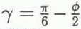. For a dihedral angle of ϕ = 32°, α _v = 0.0725.

3. The Thermal Behaviour of Polycrystalline Ice

The thermodynamics of polycrystalline ice are markedly different from that of a single crystal because it is a two-phase system. The melting point of the ice–water system depends on the pressure, the curvature of the solid–liquid interfaces and the presence of impurities. We can write for the temperature depression θ of the melting point below 0°C in a polycrystal of ice

(4)

where T₀ is the melting point of pure ice, L is the latent heat of pure water, ρ _i and ρ _w are the densities of pure ice and pure water, R is the universal gas constant, p is the excess pressure in the water and c is the impurity concentration in the water. (N.B. θ is the temperature depression below the melting point of pure ice, T₀ = 273.16 Κ = 0°C, and is therefore a positive quantity.)

By definition, a two-phase system can only be in equilibrium when it is at its melting point. A polycrystal of ice is therefore only in thermal equilibrium when its temperature is at θ below 0°C.

The experiments to be presented in this paper were conducted at atmospheric pressure and so Equation (4) reduces to

(5)

Reference NyeNye (1991a) considered the case where there are no flows in the system and assumed that the impurities are perfectly expelled from the crystal lattice and the grain boundaries. If r _sl is isotropic and hence r _v is a constant of the system as suggested in the previous section, then the concentration in the veins is given by

(6)

where M is the mass of solute per unit length of vein and is constant. Equation (5) then reduces to

(7)

where

(14)

The essential difference between the thermal behaviour of a polycrystal and that of a single crystal is encapsulated in Equation (7). The temperature depression in the polycrystal θ is expressed merely as a function of the vein size r _v. In other words, to change the equilibrium temperature of a polycrystal, we must change the vein size and so latent heat must be supplied. Reference NyeNye (1991a) showed that the heat flows in a polycrystal can be understood in terms of an effective specific heat σ _eff which contains two terms:

(9)

where σ is the specific heat of pure ice and l is the length of veins per unit volume. The second term is called the anomalous specific heat. It is a temperature-dependent term and is due to the latent-heat contribution of the veins. Nye showed that the heat-diffusion equation for a polycrystal is then

(10)

where

and is the diffusivity of heat in a pure single crystal of ice. Figure 3 shows D_eff as a function of temperature.

Fig. 3.

Ratio of the effective diffusivity of a polycrystal D_eff to the diffusivity of heat in ice D _h as a function of the temperature depression θ (after Reference NyeNye, 1991a). Schematic only; note the highly non-linear vertical scale.

The salinity and curvature contributions to the temperature depression are equal for θ = θ′ = 2A ²/B. For θ >> θ′, r _v is small, the salinity term dominates and we may write

(11)

Furthermore, as curvature effects are small, we can simplify the equation for the effective specific heat. We put A = 0 and use Equation (11) to substitute for r ² _v in Equation (9), from which

(12)

in agreement with Reference HarrisonHarrison (1972), where the transition temperature θ _t is defined as

(13)

When θ = θ _t, D _eff = D _h/2, Harrison suggested that θ _t should be used to mark the transition from cold to temperate ice.

So far, we have only considered diffusion of heat through the sample. However, diffusion of solutes also plays a role in the equilibration process. Reference NyeNye (1991a) showed that diffusion of impurities through the bulk sample is governed by a diffusivity of D _c/3, where D _c is the diffusivity of the solute in water and the factor arises because the solute can only diffuse along the veins. D _c is generally about three orders of magnitude less than D _h; for example, the diffusivity of salt in water is D _sw = 1.26 × 10^–9 m² s^–1. Therefore, when θ is large and D _eff ≈ D _h, heat diffusion is much faster than solute diffusion. However, at the other extreme, as θ tends to zero, D _eff also tends to zero. There comes a point when D _eff < D _c/3. Nye suggested that, for smaller values of θ, D _c rather than D _eff controls the approach to equilibrium. He called ice in this region deeply temperate.

We can see how the various equations relate to a typical sample that was grown in the laboratory from singly-distilled water. The radius of curvature was found to be r _v = 40 μm (vein width d _v ≈ 20 μm) at a temperature depression of θ = 0.1 deg. Using the values T₀ = 273 Κ, γ _sl = 0.034J m⁻², L = 3.06 × 10⁸ J m⁻³ and Equation (8), we get A = 3.0 × 10⁻⁸ deg m, and so A/r _v = 7.5 × 10⁻⁴ deg, which is much less than the measured value of the temperature depression. The curvature term may therefore be neglected at this temperature depression and the simplified formula Equation (11) applies. Substituting the measured values for θ and r _v into Equation (11) gives Β = θr ² _v = 1.6 × 10⁻¹⁰ deg m². The curvature term equals the salinity term when r _v = B/A which corresponds to a radius of curvature r _v′ ≈ 3.8 mm (vein width d _v′ ≈ 2.9 mm) and a temperature depression of θ′ = 2A ²/B = 1.1 × 10⁻⁵ deg.

The transition temperature θ _t requires an estimate for the total length of veins per unit volume in the sample. The grains in these samples are typically long and thin (see section 5). For grains which are about 4 mm across and 10 cm long, we have a total length of veins per unit volume of the order of l ≈ 7 × 10⁴ m⁻². Using the values α _v = 0.0725 and L/σ = 160 deg in Equation (13), we get θ_t = 0.011 deg for the transition temperature. This corresponds to a radius of curvature r _vt = 122μm (d_vt ≈ 59 μm). Now, θ _t >> θ′ and so for temperatures at least up to the transition temperature we can neglect curvature effects.

The temperature θ″ at which D _eff = D _sw/3 can be calculated from Equation (10) and Equation (7). For the typical sample, θ″ = 2 × 10⁻⁴ deg and 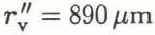(d _v ≈ 445 µm). The contribution due to curvature at this temperature depression is A/r"_v = 3.37 x 10⁻⁵ deg which is about 17% of θ″. We can see that curvature effects will become important when the diffusivity of the continuum is controlled by the diffusion of impurities along the veins.

Note that D _h = 1.19 × 10⁻⁶ m² s⁻¹ and D _sw = 1.26 × 10⁻⁹ m² s⁻¹ and so the diffusivity in a polycrystal and hence the time constant will vary, depending on the temperature, by three orders of magnitude. It would be extremely difficult to make reliable observations of changes in the equilibrium vein size with temperature in the deeply temperate region, because of the very small temperature depressions, θ < 2 × 10⁻⁴ deg, coupled with the very long time constant, which is of the order of 10 h. Consequently, all the experiments presented here look at ice in the cold to temperate region near the transition temperature where the temperature depression is controlled by the salinity term.

Now, in Equation (11), the mass of solute in the veins has been assumed to be constant. But we know that because of the volume expansion on freezing there will be flow of water along the veins out of the sample on cooling and into the sample on warming. This effect is called pumping. The result of the pumping is that the mass of the solute will not be constant. For each volume of water frozen, a fraction ϵ is expelled: ϵ = 1 − ρ _i/ρ _w = 0.083. The change in the mass of solute per unit length is then

(14)

Now, the concentration is simply c = M/α _v r ² _v. Substituting for c in Equation (14) and integrating gives

(15)

where M ₀ and r _v0 are the initial values. Combining Equations (8), (11) and (15) gives for the temperature depression

(16)

which is

(17)

where

(18)

Equation (17) shows that the effect of pumping is to reduce the exponent by 2ε = 0.166.

4. The Experimental Apparatus

The experiments were performed in a commercial walk-in freezer that was controlled to 0° ± 2°C. Figure 4 gives an overview of the experimental apparatus. A cylindrical, polycrystalline ice sample S (length 7 cm, diameter 3 cm) was suspended in a saline water bath A (capacity 1.51) The ice was clamped in the jaws of a sample holder H that was specially designed to hold and position ice. This holder has been described in detail by (Reference MaderMader 1990, Reference Mader1992). The contact pads are made of porous glass which allows any water created by pressure melting to flow away from the surface of the pads. Slip between the sample and the pad does not occur and so a piece of ice could be held immobilized for the duration of an experiment (3h). The water bath provided the sample with both a temperature and a salinity environment. It is conceptually simpler to eliminate the salinity effect and this was done by containing the ice in a plastic bag (not shown), thus isolating it from the salinity of the bath whilst maintaining thermal contact. The sample was viewed in transmission by an optical microscope M which has an attachment for a camera (not shown). A water-filled chamber F (thickness 3 cm) was placed between the white light source L (power 15W) and the mirror R, so that most of the infra-red radiation was absorbed before it reached the bath. The observation stage of the apparatus, i.e. the microscope, with lamp, filter and mirror, and the water bath, with sample, stirrer and temperature probes, were all mounted on a vibration-free tablet.

Fig. 4.

Schematic drawing of the experimental apparatus.

The temperature in the water bath was controlled by pumping water around a circuit that included another vessel Β (capacity 21) which contained a mixture of singly-distilled water and ice chips, which were also made from singly-distilled water. By adding saline solution to B, the temperature of the freezing mixture in it was lowered. Pumping this cold solution around the circuit then reduced the temperature in A. The peristaltic pump Ρ was always operated at the maximum throughput, about 370 ml min⁻¹, to minimize the time needed to change the temperature in the water bath. Both arms of the circuit could be accommodated in the pump which meant that the flow was the same around the circuit. The water levels in the two vessels therefore remained constant.

The temperature in A was kept uniform throughout the whole bath by a large stirrer (diameter 8 cm, 250 rpm). Temperatures several degrees below 0°C could be easily achieved using this arrangement. The best control of the temperature in the water bath was achieved by treating vessel Β as a supply of cold saline solution. The experimenter could add cold saline solution from Β to A via the pump, or warm water to A by hand, to achieve and maintain the desired temperature. Using this technique, the temperature in the water bath could be controlled to within ±0.0025°C.

The temperature in the water bath A was measured using a highly sensitive, integrated-circuit temperature transducer. This device acts as a high-impedance, constant-current regulator, passing 1 μΑ Κ⁻¹ with a specified linearity of ±3°C (for the AD590(IF) version of the transducer) over the full operating temperature range from −55° to + 150°C (for a detailed circuit description see Reference TimkoTimko (1976)). The output of the device is thus proportional to absolute temperature (PTAT). Figure 5 shows a simplified circuit diagram of the electronics associated with the temperature transducer. A stabilized ±15V supply is used to power the temperature probe, the reference voltage chip and a × 100 differential amplification stage. The resistor R _t (nom. R _t = 10 kΩ) converts the PTAT current output of the probe into a PTAT voltage V_s (nom. T × 10 mV K⁻¹). The reference voltage V _r (nom. + 2.732 V) provides the voltage appropriate to the zero of the Centigrade scale, 273.2 K, so that the difference V _s − V _r is a measure of the Centigrade temperature T′. After amplification, the final nominal output is V ₀ = Τ′ × 1 V °C⁻¹.

Fig. 5.

The electronics associated with the temperature measurement. (See text for definition of symbols.)

The calibration process involves setting the resistance R _t such that the signal voltage V _s = +2.732 V at T′ = 0°C. This is done by first setting the reference voltage to V_r = +2.732 V. The probe is then held in a well-stirred bath that contains a freezing mixture of distilled water and very small, distilled-water ice chips and the resistors are altered until the ouput V ₀(0°C) = 0 V, i.e. V _s(0°C) = V _r = + 2.732V. The probes are subject to self-heating effects which are eliminated from the measurement by calibrating the probes in an environment that is similar to the test environment. The calibration and test environments are similar here because they are both well-stirred water baths. The actual values after calibration were V _r = + 2.730 V and V ₀(0°C) = + 0.150 V, hence V _s(0°C) = 2.7315 V. Centigrade temperatures appear as voltages measured relative to V ₀(0°C) with a voltage temperature coefficient of 1 V°C⁻¹.

The accuracy of the temperature measurements is limited by the linearity of the device itself (max. 1.5%), by a possible error in the amplification (the resistances associated with the operational amplifier have tolerances of 0.1% giving an error of max. 0.2%), and by the calibration error. These three sources of error combined result in a scale-factor error, which causes a deviation in the final temperature-voltage coefficient from the ideal value of 1V °C⁻¹. The calibration error was 0.5mV, which gives a scale-factor error of only 0.02% due to calibration. The total scale-factor error is 1.72% and may be assumed constant.

The electronics were thermally insulated, but changes in the thermal environment of the electronics over long periods of time cause a slow drift in the value of V ₀(0°C). A knowledge of V ₀(0°C) is necessary, if we are to measure particular temperatures accurately. V ₀(0°C) was measured before and after each experiment using the calibration set-up. If the value had altered, then V ₀(0°C) at a particular time was deduced using linear interpolation. The linear approximation is highly accurate and the error on V ₀(0°C) is expected to be << 1%. Consequently, if we know how V ₀(0°C) changes with time, then the accuracy of a particular measurement of temperature is again limited by the total scale-factor error, max. 1.72%. In practice, a limit to the temperatures that could be measured was provided by the resolution of the voltage-detecting equipment. It is possible to resolve voltages of ±2.5 mV = ±0.0025°C on the chart-recorder trace.

Vein widths were determined from photographs of the veins taken using the microscope. The method was the same as in Reference MaderMader (1992). Measurements were taken off prints rather than directly off the negatives. Distances between two lines on a print can be determined to within about ±0.25 mm, i.e. about 1.4 µm at the maximum magnification of about × 180. This is therefore the resolution limit and is a consequence mainly of the graininess of the negative. Veins with apparent widths of less than about 3 μm therefore could not be resolved, as the vein edges start to overlap on the negative at this stage. Also, diffraction effects start to become important for such small veins.

5. The Samples

Clear, stress-free polycrystalline ice samples were grown in the laboratory by lowering a plastic bag filled with singly-distilled water into a freezer at a rate of 15 cm d⁻¹. The temperature in the freezer was −27°C. The resulting ice columns were typically about 45 cm long and 3.2 cm in diameter. The grain structure within the columns showed strong signs of preferential grain growth; the grains were typically long and thin and the grain-size in planes perpendicular to the direction of growth was seen to grow with height. The ice-growing technique and the grain structure have been described in more detail in Reference MaderMader (1992).

The distribution of the ionic impurities in the columns was investigated by measuring the electrical conductivity of meltwater samples taken from different regions in the columns (Reference MaderMader, 1990). The analysis shows that 89 ± 8.9% of the impurities reside in only 14.5 ± 1.5% of the volume, namely, within about 1 mm of the curved surface and in roughly the top 2 cm of the ice column, the last part of the column to freeze. The bulk of the ice is therefore very pure. An impurity concentration analysis was carried out by British Antarctic Survey chemists on a melted sample of polycrystalline ice taken from one of the ice columns. The central part of the ice sample was used in this analysis; the dirty surface layer had been melted away. Their measurements produced the values shown in Table 1. The bulk impurity concentration c _b, is of the order of 10⁻⁶ mol l⁻¹ and is consistent with the value estimated from the conductivity measurements (Reference MaderMader, 1990).

Table 1.

Results of impurity analysis performed on the core of a sample grown from singly-distilled water (courtesy of the British Antarctic Survey)

Na⁺ not measured. Thus, a typical salt of about 0.7 × 10⁻⁶mol l⁻¹.

The ice from the ice columns is similar in grain-size and bulk-impurity concentration to natural ice samples. Reference Harrison and RaymondHarrison and Raymond (1976) quoted values for natural ice samples from Blue Glacier, Mount Olympus, U.S.A.: fine ice (grain-size 1–3 mm) c _b ≈ 3 × 10⁻⁶ mol l⁻¹, and coarse ice (grain-size 10–30 mm) c _b ≈ 0.8 × 10⁻⁶ mol l⁻¹.

Ice columns were also grown from dilute solutions containing known impurities. NaCl and H₂SO₄ were the chosen dopants as these are common impurities in natural ice and also because there is evidence to suggest that acids congregate preferentially in the veins whereas salts do not (Reference Davies, Vincent and BrimblecombeDavies and others, 1982; Reference Wolff, Mulvaney and OatesWolff and others, 1988).

Ice samples 5–7 cm in length were taken from the ice columns. The preparation of these samples prior to an experiment has been described in Reference MaderMader (1992). The preparation process was called rotting. It involved placing the samples in individual, sealed plastic bags and immersing them in a freezing mixture for periods of days or weeks. The temperature of the freezing mixture was probably marginally below 0°C primarily because of residual impurities in the flask. In any case, it was always higher than the temperature of the samples at the time of immersion. During rotting, the temperature in the samples therefore increased and the veins grew. It was noted in Reference MaderMader (1992) that the vein size grew fast at first but, by the time a vein width of 100μm or more had been reached, the process was much slower. Samples could be kept for many days at this stage with very little change in the vein size. The vein width after a long time t depends on the temperature of the freezing mixture and on the mass of solute per unit length of vein in the vein system.

Table 2 shows the mean vein width after rotting of the nodes observed in experiments 1–4 (see section 7). A comparison of samples 1 and 2 is possible as they were taken from the same ice column and were rotted in the same flask. The measured vein width was essentially stable after 17 d. Comparison of these samples with the others is more difficult as samples 3 and 4 derived from different ice columns and were rotted in different flasks. The much larger vein size measured for sample 4 is thought to be primarily due to a higher mass of solute per unit length of vein in this sample than in any of the others (see section 8) rather than the longer rotting time.

Table 2.

Effect of rotting process on the samples studied in section 7.

The rotting situation described here is different from that studied by Reference NyeNye (1991b). In Nye’s model, the sample is in direct contact with a bath of fixed temperature and concentration rather than having only thermal contact. Nye, therefore, had to take account of diffusion of solutes between the bath and the sample. The resulting expression for the asymptotic (t → ∞) growth of the veins has the time dependence . It contains no adjustable parameters and is independent of the concentration of the surrounding bath and of how the process starts. As diffusion of solutes from the veins to the bath (or vice versa) is not possible in the rotting situation described in this paper, this asymptotic solution will not be reached. The mass of solute per unit length of vein is constant with time, provided the surface of the sample remains dry. This was generally the case for my samples as they were isolated from the freezing mixture, which was itself very pure, and so the differences between the samples were maintained during the rotting process.

6. Experimental Method

The experiments study the vein size as a function of temperature. We are only concerned with the conditions at thermal equilibrium. The temperature in the water bath was repeatedly altered. At each temperature, the sample was allowed to equilibrate for at least 3 min before a photograph was taken and the temperature in the water bath was measured. In thermal equilibrium, the temperature in the veins is the same as the temperature in the water bath.

The vein was in each case only photographed from one direction. If the equilibrium vein-system geometry was uniform, then the radius of curvature of the vein walls r _v could be calculated directly from the distances between the vein edges seen on the photograph. However, we have noted that the equilibrium vein-system geometry is generally non-uniform. Therefore, to gain a better estimate of r _v, the vein was usually photographed near a node. The radius of curvature was calculated independently for each vein observed using the equations derived for a uniform vein system. The average of these values r _v is the best estimate and the spread of the values indicates the likely error on the calculation.

7. Results

7.1. Experiments on Ice Grown from Singly-Distilled Water

The results of two experiments using samples that were grown from singly-distilled water are summarized in Figure 6 and 7. Each figure shows a photograph of the vein system observed and a graph of the vein size as a function of the temperature depression in the veins. The numbers next to the points on the graphs indicate the order in which the observations were made. In each experiment the samples were cooled, then warmed up again before being cooled once more. A number of data have been excluded from the graphs because the temperature measured in the water bath was above 0°C which is not an equilibrium condition as the temperature in the veins is always below 0°C. This applied to the starting point of both experiments. Also, the temperature in the water bath rose above 0°C during the warming phase between points 11 and 12 of experiment I. After the starting point of experiment 2, the temperature in the water bath was always below 0°C, which means that points 11 and 12 describe the conditions in the veins during the warming phase of the experiment. In both experiments, there has been an increase in vein size from the first to the second cooling phase. The lines drawn through the data points are the lines of best fit for each of the cooling phases. The main difference between the curves lies in the value of the constant C in the general equation θ = Caⁿ .

Fig. 7.

Results of experiment 2. (a) Photograph of the rotted vein system in a sample grown from singly-distilled water. Veins 3 and 4 are superimposed. The node can be assumed to have uniform geometry because the values for the radius of curvature calculated independently for veins 1 and 2 using Equation (1) and (2) are within the error of each other. (b) Graph of the temperature depression θ in the veins as a function of the apparent vein width a of vein 1. At the start of the experiment, the apparent width of vein 1 was a = 100 ± 2μm. This point is not shown as the temperature in the bath exceeded 0°C. The lines of best fit are of the form θ = Caⁿ and have the following errors associated with them: first cooling curve n ± 7% and C ± 21%, and second cooling curve n ± 4% and C ± 12%. Note the temperature oscillation between points 13 to 17.

7.2. Experiments on Ice Containing known Impurities

The results of two experiments using samples that were grown from solutions containing a known impurity are summarized in Figure 8 and 9; in experiment 3 the solution contained 10_–4 mol l^–1 NaCl and in experiment 4 10_–4 mol l^–1 H₂SO₄. The experiments were conducted in the same way as those presented in section 7.1.

Fig. 9.

Results of experiment 4. (a) Photograph of the rotted vein in a sample grown from a solution containing 10⁻⁴ mol l⁻¹ H₂SO₄. A node at one end of this vein was noted to be similarly regular in appearance to that observed in experiment 1. Therefore, the radius of curvature calculated for this vein using Equation (1) and (2) is probably accurate to within about ± 10%. (b) Graph of the temperature depression θ in the vein as a function of the apparent vein width a. At the start of the experiment, the apparent width of vein 3 was a = 343 ± 2 μm. This point is not shown as the temperature in the bath exceeded 0°C. The line of best fit is of the form θ = Caⁿ and has the following errors associated with it: n ± 7% and C ± 6%.

In experiment 3, there were insufficient observations during each cooling phase to allow an accurate curve fit. The lines drawn through the points are derived assuming θ ∝ a^−1.834. Unlike in experiments 1 and 2, there has been a decrease in the value of the constant C between the first and second cooling phases. In experiment 4, the sample was cooled only once. The value of C is an order of magnitude higher for this sample than for the previous samples.

7.3. Distorted Vein-System Geometries

At the outset of most of the thermal experiments, the temperature in the water bath exceeded 0°C. It has been noted that this is not an equilibrium condition. The shape of the nodes is sometimes seen to be distorted from the expected equilibrium shape. Experiment 5 is a test of the assertion that such a distorted nodal shape is a non-equilibrium configuration. The approach was simply to take such a distorted node, lower the temperature in the water bath to below 0°C, and then watch what happens to the shape. If our assertion is correct, then, as the sample reaches equilibrium, the distortions should disappear.

Figure 10 shows a node observed in a sample grown from a solution containing 10⁻² moll−1 NaCl. The photograph was taken at the outset of the experiment when the temperature in the water bath was slightly above 0°C. The nodal shape is very distorted. The apparent vein widths change with the distance from the node. Also, the arrow in the figure indicates a point on one of the vein edges of vein 4 where the curvature of the vein edge appears to change sign. It is unclear from the photographs what the detailed shape of the vein walls look like. The approach to equilibrium geometry of the node was observed and the results of the experiment are shown in the photographs of Figure 10 and c.

Fig. 10.

Results of experiment 5. (a) The distorted nodal structure (arrow) at the outset of the experiment when the temperature in the bath was above 0°C. (b) The temperature in the water bath was dropped to −0.105° + 0.005°C. The photograph shows the node after it had been held at this temperature for 10 min. Already, the distortion indicated by the arrow has disappeared and vein 3 has a constant apparent vein width along its length of a = 160 ± 2μm. However, veins 1 and 4 still have sizes that vary with the distance from the node. The sample was held stable at −0.105° ± 0.005°C for a further 15min, by which time the apparent width of vein 3 was a = 31 ± 2µm. Vein 1 was seen to have a constant apparent width along its length, and the variation in size of vein 4 was smaller although still evident, (c) The temperature in the water bath was raised to −0.030° + 0.005°C and after a further 15min this photograph was taken. The apparent width of vein 3 is now a = 63 ± 2 µm. The nodal shape is much closer to that expected. The variation in the apparent width of vein 4 persists, but is significantly reduced compared to that observed at the outset.

Experiment 6 (Fig 11) studied the behaviour of another example of a local distortion of the geometry of the vein system which was seen gradually to even out during the course of the experiment. The sample used had been grown from a solution containing 10⁻⁴moll⁻¹ NaCl. On scanning through the sample, two nodes were seen located about 2 cm from the front flat face. The initial observation was that the vein connecting the nodes had a dramatically different apparent width at each end. Also, in the immediate vicinity of each node, the vein size appeared to be constant with the distance away from the node. Scanning along the whole length of the interconnecting vein, the discontinuity shown in Figure 11 was discovered. The temperature in the water bath was varied and the behaviour of the vein in the vicinity of the discontinuity observed. The results are shown in Figure 11b and c.

Fig. 11.

Results of experiment 6. (a) This photograph was taken immediately after the temperature in the water bath had been dropped to −0.15° ± 0.02°C. The apparent vein width changes extremely suddenly from a = 16 ± 2 μm to a = 69 ± 2μm, i.e. by more than a factor of 4. (b) The water bath was then allowed to warm up to −0.11° ± 0.02°C over a period of about 30 min, at which point this photograph was taken. The discontinuity has already been replaced by a gradual change in the size of the vein along its length, from a = 59 ± 2μm to a = 22 ± 2μm. Note that the vein has actually frozen at the wider end despite the rise in temperature, (c) The temperature in the water bath was once more reduced to −0.127° ± 0.005°C, before being allowed to warm up again over a period of 45 min to −0.031° ± 0.030°C. The photograph shows the connecting vein at this point. There is still a variation in the apparent width along the vein from a = 113 ± 2μm to a = 91 ± 2 μm, but the change is gradual and by a factor of less than 2. After a further 50 min, the temperature in the bath was −0.090° ± 0.005°C and the variation in the vein-size was no longer observable. The apparent vein width was a = 22 ± 2 pm along its length.

8. Discussion and Conclusions

The cooling curves of experiments 1 to 4 are in agreement with the theoretically derived behaviour; from Equation (17), we have θ = C′r ^−1.834 _v and, as r _v ∝ a, then θ = Ca ^−1.834. The mass of the solute in the veins is only modified by the action of pumping. Experiments 1, 2 and 4 have sufficiently many points to allow the value of the exponent to be deduced from the data. We have five independent measurements of n from these three experiments — see Table 3. The mean value is n = −1.82±0.02, which is in agreement with the theoretical prediction. Experiment 3 provides additional data that are also consistent with an exponent of n = −1.834.

Table 3.

Measurements of the exponent n

It is important to distinguish carefully between the quantities Β and C′, or C. We see from Equation (8) that B is a measure of the mass of the solute per unit length of vein M. Now, C ∝ C′ and Equation (18) shows that C is also related to the mass of the solute per unit length of the vein, but it is a measure of the ratio M/r ^2ε _v. The temperature versus vein-size behaviour follows lines of constant C. These lines cut across lines of constant Β such that Β increases as the temperature depression decreases. Β and hence M are therefore temperature-dependent variables because of the action of pumping.

The cooling curves all follow the same functional form but values of C can vary, which implies that the ratio M/r ^2ε _v is different; that is, the value of M at a particular vein size (or temperature depression) is different. Generally, a change from one value of C to another is observed during the warming phase in an experiment. This is a secondary effect of pumping. When the sample is warmed up and the veins melt, water is sucked into the vein system from the surface of the sample. The impurity content in this water is, in general, different from that in the veins. Some of these impurities are imported into the vein system during the melting process.

The most frequent observation is of an increase in C, as in experiments 1 and 2. This is consistent with the fact that the impurities tend to congregate at the surface of the ice columns. In experiment 3, C was observed to decrease on melting. This sample had been treated rather differently from the others; the grain structure had been observed by placing it between crossed polaroids. During this process, melting occurred and so it is possible that a lot, if not all, of the contaminated surface layer was lost before the measurements were made.

Pumping, which is responsible for the increase in the exponent, should be observed throughout the vein network and during all temperature changes in these samples. But, at what point, or indeed whether, a change in the constant C is observed depends on the temperature change involved and on how far away from the surface, via the vein network, the observation point is. This is a consequence of the fact that the diffusion of solutes along the veins is small compared to the other processes involved. The change in C relies on the impurities being carried by a flow of water and solutes from the surface. The flow must reach as far as the observation point, which was as much as 2 cm or so from the surface. This deserves further investigation as it is not self-evident that the effect will be so large.

Further Considerations of Pumping

It is simpler, when discussing pumping, to consider the flow in a vein on freezing as this is a well-defined situation. The melting process is physically simply the reverse, but with the added complication of an unknown source of water and impurities at the surface of the sample.

We consider the simplest case of a single vein running down the length of a cylindrical sample, as shown in Figure 12a. The vein has a uniform cross-sectional area A _v. The solution in the vein has a uniform impurity concentration and is assumed to be incompressible. As the temperature of the sample is lowered, vein water freezes thereby reducing the cross-sectional area of the vein by an amount dA _v. The fractional expansion of water on freezing causes some of the water to be expelled at the outcrops. Obviously, the situation is symmetrical and so only one-half of the sample need be considered, as in Figure 12b.

The volume of water per unit length of vein that is expelled is simply εdA _v. In Figure 12, the expelled water is drawn as if still confined to an imaginary vein that has the same cross-section as the real vein. This is merely a constructional device. We consider the pocket of water that initially fills the vein from the midpoint to a coordinate at x which moves with the water as the vein cross-section expands and contracts. If the cross-sectional area of the vein reduces by dA _v, then the front of the pocket will move by dx, which is given by

(19)

Fig. 12.

Idealized motion of a front at x = x₀ due to volume expansion on freezing, (a) Vein before freezing with the cross-sectional area A_v and (b) after freezing with the cross-sectional area reduced by an amount dΑ_v.

We denote the initial and final values for A _v as A _vi and A _vf, and observe the total motion of a front that is initially at x = x ₀, i.e. when A _v = A _vi. Integrating Equation (19) we get

(20)

To get an idea of the scale of the effect, we can substitute in some typical values. We take the case of an experiment where the vein size changes from d _v = 60 μm to d _v = 10 μm. This is a change in A _v from A _v ≈ 10⁻⁹ m² to A _vf ≈ 10⁻¹¹ m⁻². Using ε ≈ 0.1, we get x ≈ 1.50x ₀. For a sample such as in experiment 1 which was about 8 cm long, the face at x ₀ ≈ 2.6 cm has been moved all the way to the outcrop at x as 4 cm. There has been a complete exchange of solution within the region 2.6 cm < x < 4cm. The situation on melting is the reverse; for observations made in the region 2.6 cm < x < 4 cm, we can expect to observe the influx of water and impurities from the surface.

On the basis of this very simple model, we would expect the influx of impurities at a particular observation point, i.e. the change from one curve of constant C to another, to be sudden. Also, the model, when followed through, implies that the process is completely reversible. Figure 13 shows a sketch of the temperature depression versus vein-size behaviour in a typical sample. The initial cooling cycle takes us from point A to point Β along the curve with constant C = C ₁. Warming the sample up again, we expect to follow the same curve back again up to a point P, which is when the influx of impurities from the surface reaches the observation point. The changeover to the new curve with C = C ₂ happens suddenly according to this model, taking us to point D. Now, when the sample is cooled again, our experimental observations follow the new curve to point E, whereas this model would take us back via point Ρ to point B.

Fig. 13.

Temperature depression versus vein-size behaviour in a typical vein.

The problem arises because the model assumes a plug flow; the velocity gradient across the vein is taken to be zero. This kind of flow occurs only in non-viscous situations. However, the flow here is highly viscous, as is indicated by the extremely small value of the Reynolds number Re = lV ρ/η ≈ 10⁻⁹, where ρ is the density of water (ρ ≈ 10³ kgm⁻³), η is its viscosity (77 ≈ 10⁻³ Pas), V is the mean velocity of the fluid in the veins (V ≈ 2 cm (3 min)⁻¹ ≈ 10⁻⁴ m s⁻¹; 2 cm is the typical distance to the observation point and 3 min is the equilibration time), and l is a typical length associated with the vein cross-section (l ≈ d _v ≈ 10⁻⁵ m). There will be a velocity profile with faster fluid at the vein axis and stationary fluid at the vein walls. This will modify our view in a number of ways:

• 1. Solution from the surface will be imported even deeper into the sample than implied by the simple model.

• 2. Different streamlines will have different impurity concentrations associated with them. There will be a concentration gradient across the vein.

• 3. The concentration gradient will drive diffusion of the solutes in the plane of the vein cross-section. The diffusivity of salt in water is D _sw ≈ 10⁻⁹ m ² s⁻¹ and is large enough to produce a uniform concentration over the vein cross-section d _v ≈ 10⁻⁵ m) in the usual equilibration time (τ sa ≈ 3 min).

The effect on the observations will be two-fold:

• 1. The change-over from one line of constant C to another will not be as abrupt as is implied by our simple model. In Figure 13, the line from P′ to D indicates the expected behaviour when this modification is included. This is consistent with the observations. In general, the changeover is sufficiently sudden that it was not possible to get measurements covering the P′ to D behaviour. All the points lie on one or other of the curves. However, in experiment 2, points 11 and 12 show the change-over.

• 2. The situation will not be reversible, because of the diffusion of solutes in the plane of the vein cross-section. Therefore, the vein behaviour on cooling will not return from D via P’ to Β but will proceed, as observed, from D down the line of constant C = C ₂ to point E.

The Effect of the Doping Agents

It is possible to calculate the mass of solute per unit length of vein M for a data point (θ, r _v). From Equation (17) and (18), we get

(21)

The value of M for θ = 0.1 deg has been determined for our samples. M ≈ 10⁻⁸ mol m⁻¹ for samples grown from singly-distilled water and also for samples grown from doubly-distilled water doped with small amounts of NaCl (10⁻⁴ mol l⁻¹ or 10⁻²mol l⁻¹). Samples grown from a solution of doubly-distilled water and 10⁻⁴mol l⁻¹H₂SO₄ produced a sample with a significantly higher mass of solute in the liquid phase, namely M ≈ 10⁻⁷ mol m⁻¹ for θ = 0.1 deg.

The value of M for samples grown from NaCl-doped water appears to be independent of the impurity concentration of the NaCl dopant in the solution from which the samples were grown; the two samples considered in experiments 3 and 6 came from solutions with impurity concentrations that are different from each other by two orders of magnitude, but the response of both these samples to changes in temperature was similar to that of samples grown from singly-distilled water. This suggests that the contamination level in the bulk crystal (that is, the impurities contained within the grains, in the grain boundaries and in the veins) was roughly the same for all these samples and that the majority of the impurities were located at the ice surface, as in the case of the ice columns grown from singly-distilled water. The additional impurities contained in the ice colums grown from the highly doped solution (10⁻²mol l⁻¹ NaCl) were most probably located at the ice surface, though there are no independent measurements to support this.

Given a knowledge of the mass of the solute per unit length of veins, typically M ≈ 10⁻⁸ mol m⁻¹ and the length of veins per unit volume of the ice, typically l ≈ 10⁵ m⁻², we can estimate the impurity concentration per unit volume due to the impurities in the veins, C _v = M × l ≈ 10⁻³ mol m⁻³ = 10⁻⁶ mol l⁻¹. Comparing this value with the estimates of the bulk impurity concentration (C _b in section 5, we see that it is possible for all the impurities in the samples to be contained in the veins.

9. Summary

The functional form of the temperature versus vein-size behaviour of the veins has been determined. The experiments have shown that θ = Ca ⁿ where ñ = —1.82 ± 0.02, θ is the temperature depression in the vein, a is the apparent vein width and C is a constant. This relationship implies that the mass of the solute per unit length of vein M remains in the liquid phase during a temperature change. In the theoretical derivation, it was assumed that the solid phase is pure and that no solute is incorporated into the ice lattice when the veins freeze. By taking account of the density change that occurs during a phase change, we obtained the relationship θ = C′r _v ^−1.834 = Ca ^−1.834 which is in agreement with the observations.

From the derivation, we found that the constant C ∝ M/r _v ^0.166. The mass of the solute per unit length of vein therefore varies with the vein-size. We have shown that this is solely an effect of the difference in the density of water and ice. The volume expansion (contraction) on freezing (melting) causes a flow of water and hence impurities and thereby leads to a decrease (increase) in M that is proportional to r _v ^0.166. This effect occurs over the whole temperature range. Furthermore, we have found that during the melting process the flows provide a mechanism for the transport of impurities from the sample surface into the vein system. The effect of this pumping on the vein system is, in general, to change the value of the constant C. That is, the mass of the solute per unit length of vein at a given vein size is altered. In our experiments, C generally increased, which is consistent with the fact that the samples were found to have a highly impure surface layer.

The influx of impurities from the surface is important in these samples, mainly because of their small size. In a large body of ice, such as a glacier, the effect would be peripheral. However, the M ∝ r _v ^0.166 variation is independent of the location of the observation point, and so we would expect this to occur throughout a glacier.

The value of M for θ = 0.1 deg has been determined for our samples. We found that M ≈ 10⁻⁸ mol m⁻¹ for samples grown from singly-distilled water. Similar experiments were performed on pure samples doped with small amounts of NaCl or H₂SO₄. The same general behaviour was observed but, in the case of the H₂SO₄-doped samples, we found that M was an order of magnitude greater. These measurements support the idea that acids are concentrated preferentially in the veins. Similar results have been reported in natural polar ice by other workers (Reference Mulvaney, Wolff and OatesMulvaney and others, 1988; Reference Wolff, Mulvaney and OatesWolff and others, 1988) using scanning electron-microscopy techniques. High concentrations of acids in the vein system can correctly predict the d.c. conductivity of polar ice (Reference Wolff and ParenWolff and Paren, 1984) and can explain the release of strong acids by melting snow reported by Reference Davies, Vincent and BrimblecombeDavies and others (1982).

The theory of Reference NyeNye (1989) studies the coupled heat and solute diffusion problem of the vein system in the polycrystal. The essential assumption in this theory is that the solute remains in the liquid phase during a phase change. Our observations have shown this to be true. Nye’s theory only differs from the experimental situation in that it neglects all flows.

A consequence of Nye’s continuum approach is that the effective diffusivity of a polycrystal of ice D _eff is strongly temperature-dependent, which is in agreement with Reference HarrisonHarrison (1972). D _eff varies by three orders of magnitude. This is a direct result of the latent heat required for melting or freezing at the vein walls during temperature changes and is not altered by the effects of pumping. The variation with temperature has been observed during the rotting process where the vein size was noted to grow increasingly slowly as the sample warmed up, indicating a gradually increasing diffusivity.

The diffusivity of solutes in water is three orders of magnitude less than the diffusivity of heat in ice. Also, the contribution to the temperature depression of the curvature term is much less than that due to the salinity term in these experiments. Nevertheless, it is important to include both these effects in a discussion of vein-system behaviour. This has been clearly demonstrated in experiments in which the behaviour of distorted veins has been observed. The approach to equilibrium vein-system geometry is controlled by the diffusion of solutes along the veins. Temperature changes in a system that has reached equilibrium geometry are governed by D _eff, that is heat diffusion, alone for all values of θ.

Both the observation and the theory we have given to explain them apply where the contribution to the temperature depression of the the curvature term is negligible compared to that of the salinity term. We have found that in a typical sample this is when θ >> 10⁻⁴ deg, which covers both the cold and the temperate regions. The temperatures in our experiments were in the range 0.005 deg < θ < 0.500 deg and are typical of the temperatures measured in a temperate glacier (Reference Harrison and RaymondHarrison, 1975). Furthermore, an investigation of the samples grown in the laboratory has shown them to have a similar grain-size and bulk impurity concentration to samples of natural ice from a temperate glacier.