


1. Introduction
Flow field measurements in the atmospheric boundary layer (ABL) have relevance for a broad spectrum of applications, ranging from fundamental turbulent boundary-layer research (Gal-Chen, Xu & Eberhard Reference Gal-Chen, Xu and Eberhard1992; Menut et al. Reference Menut, Flamant, Pelon and Flamant1999), to analysing turbulent wakes of wind turbines (Käsler et al. Reference Käsler, Rahm, Simmet and Kühn2010; Iungo, Wu & Porté-Agel Reference Iungo, Wu and Porté-Agel2013; Rhodes & Lundquist Reference Rhodes and Lundquist2013) to air quality studies (Wakimoto & McElroy Reference Wakimoto and McElroy1986), among others. Pulsed light detection and ranging (lidar) sensors allow taking flow field measurements almost simultaneously at multiple locations in space, at frequencies of around one Hertz, leading to a vast amount of measurement data (Peña & Hasager Reference Peña and Hasager2011). However, lidar sensors are limited to measuring the velocity component in the direction of the beam, the so called line-of-sight wind speed.
Several techniques exist for transforming these raw data into velocity vectors. A first category only deals with time-averaged flow statistics, based on the estimation of the parameters of an analytical wind speed model (see e.g. Aitken et al. Reference Aitken, Banta, Pichugina and Lundquist2014; Borraccino et al. Reference Borraccino, Schlipf, Haizmann and Wagner2017). In a second approach, the instantaneous velocity is reconstructed but only at discrete measurement points in space using simple algorithms to transform the measured wind speeds to velocities, e.g. assuming horizontal homogeneity, and stationarity of the velocity field between the measured points in combination with Doppler beam swinging lidar scan mode (Lundquist et al. Reference Lundquist, Churchfield, Lee and Clifton2015), or assuming zero spanwise and vertical velocity in combination with a spinning lidar (Simley et al. Reference Simley, Pao, Frehlich, Jonkman and Kelley2011; Mikkelsen et al. Reference Mikkelsen, Angelou, Hansen, Sjöholm, Harris, Slinger, Hadley, Scullion, Ellis and Vives2013; Schlipf, Schlipf & Kühn Reference Schlipf, Schlipf and Kühn2013).
All the previous approaches ignore the spatial correlations of the turbulent flow field, which are, e.g. known to extend up to  $20$ times the boundary-layer height in the streamwise direction for neutrally stratified ABLs (Fang & Porté-Agel Reference Fang and Porté-Agel2015). In three-dimensional variational data assimilation (3D-Var), these correlations are taken into account (Lorenc Reference Lorenc1981); a similar method named linear stochastic estimation has been simultaneously developed in the turbulence community (Adrian Reference Adrian1979; Adrian & Moin Reference Adrian and Moin1988). Recently, this has been applied to microscale flow fields (Krishnamurthy et al. Reference Krishnamurthy, Choukulkar, Calhoun, Fine, Oliver and Barr2013; Bos, Giyanani & Bierbooms Reference Bos, Giyanani and Bierbooms2016; Dimitrov & Natarajan Reference Dimitrov and Natarajan2017). In these last studies, the velocity correlation is modelled using a three-dimensional (3-D) homogeneous isotropic turbulence spectral correlation tensor. This is often justified in the horizontal directions; however, in boundary layers, the vertical direction shows strong anisotropic behaviour. A method to incorporate the time series of measurements for nonlinear systems has been independently and simultaneously developed in the geoscience and control community and is known as four-dimensional variational data assimilation (4D-Var) (Lewis & Derber Reference Lewis and Derber1985; Le Dime & Talagrand Reference Le Dimet and Talagrand1986; Lorenc Reference Lorenc1986; Talagrand & Courtier Reference Talagrand and Courtier1987) and nonlinear moving horizon state estimation (Jang, Joseph & Mukai Reference Jang, Joseph and Mukai1986), respectively in the two communities. This methodology minimises a linear combination of the mismatch between a time series of real and virtual observations, the model error, and the deviation from the background distribution.
The combination of large-eddy simulations (LES) and 4D-Var with lidar data to retrieve turbulent structures was first proposed in Lin, Chai & Sun (Reference Lin, Chai and Sun2001) conducting a series of twin experiments. Later in a series of papers this methodology was applied to a field measurement campaign, using two different lidars for reconstruction and validation of the methodology (Chai & Lin Reference Chai and Lin2003; Chai, Lin & Newsom Reference Chai, Lin and Newsom2004; Newsom & Banta Reference Newsom and Banta2004; Newsom et al. Reference Newsom, Ligon, Calhoun, Heap, Cregan and Princevac2005; Xia et al. Reference Xia, Lin, Calhoun and Newsom2008). To regularise the problem, a Laplacian-based penalty term was used. Continuity was not strictly enforced but added as an additional penalty term. The combination of 4D-Var with Taylor's frozen turbulence (TFT) model was shown in Raach et al. (Reference Raach, Schlipf, Haizmann and Cheng2014), however, in this work, spatial regularisation was not included.
In the current work, LES-based reconstruction of turbulence from lidar measurements is further investigated for the ABL, improving on the problem formulation. To this end, regularisation of the problem is based on the background covariance tensor, following a Bayesian inference framework. Moreover, we transform the problem into a Karhunen–Loève (KL) basis (or proper orthogonal decomposition (POD) basis), which is constructed from the covariance tensor. This leads to an unconstrained optimisation problem, since the POD basis is by construction divergence free. Moreover, in this case, the regularisation part of the optimisation problem generally leads to a better conditioned optimisation problem (Haben, Lawless & Nichols Reference Haben, Lawless and Nichols2011), which is known to speed-up the convergence of the Limited-memory Broyden–Fletcher–Goldfarb–Shanno (L-BFGS) optimisation method, used in this study (Nocedal & Wright Reference Nocedal and Wright2006, p. 180). We further restrict ourselves to horizontally homogeneous flow, which allows for an efficient computation and storage of the POD basis, since the modes correspond to Fourier modes in horizontal directions. We test the methodology based on virtual lidar measurements in fine-grid reference simulations, using a coarser LES reconstruction grid, as well as a smaller domain. This allows us to perform detailed out-of-sample comparisons of the reconstructed turbulence with the reference solution.
The paper is further organised as follows. In § 2, the lidar observation model is described. Section 3 discusses the state estimation methodology. Subsequently, § 4 introduces the LES and TFT models used for the state estimation. The adjoint-based optimisation methodology is discussed in § 5, and details of the case set-up are introduced in § 6. Results are presented in § 7; conclusions and future outlook in § 8.
2. Lidar measurements
Lidar sensors measure the velocity component along the laser beam direction. Here, we focus on pulsed lidar sensors, which measure the wind speed at different locations along the beam simultaneously (Peña & Hasager Reference Peña and Hasager2011). An example is the Lockheed Martin WindTracer (Krishnamurthy et al. Reference Krishnamurthy, Choukulkar, Calhoun, Fine, Oliver and Barr2013), which is considered in the current work as a reference. This lidar has a range gate width of  $\Delta r=105\ \textrm {m}$, a pulse length, defined as the full width at half-maximum, of
 $\Delta p_{1/2}=105\ \textrm {m}$, an initial blind zone of
 $r_0=436\ \textrm {m}$ and a total of
 $N_r=100$ range gates, see table 1 for a summary.
Summary of the lidar parameters of a Lockheed Martin WindTracer (Krishnamurthy et al. Reference Krishnamurthy, Choukulkar, Calhoun, Fine, Oliver and Barr2013).

Consider a lidar system mounted at location  $\boldsymbol {x}_{{m}}$ (extension to multiple lidar systems is straightforward, but not considered here), and a beam direction
 $\boldsymbol {e}_{{l}}(t)$ that follows a scanning pattern in time. The lidar measurement locations then correspond to
 \begin{equation} \boldsymbol{x}_{i}(t) =\boldsymbol{x}_{{m}}+(r_0+\Delta r(i-1))\boldsymbol{e}_{{l}}(t),\quad i=1,\ldots, N_r. \end{equation}
Due to the finite pulse, range gate width and sampling time, the space–time filtered wind speed around  $\boldsymbol {x}_{i}$ is measured, oriented in the direction of the lidar beam. For a single location, we can express (Banakh, Bodaruev & Smalikho Reference Banakh, Bodaruev and Smalikho1997)
 \begin{equation} h_{n,i}(\boldsymbol{u}(\boldsymbol{x},t)) \triangleq \frac{1}{T_{{s}}}\int_{t_{n-1}}^{t_n}\int_{\varOmega} \boldsymbol{u}(\boldsymbol{x},t)\boldsymbol{\cdot} \boldsymbol{e}_{l}(t) \ \mathcal{G}({\boldsymbol{\mathsf{Q}}}(t)(\boldsymbol{x}-\boldsymbol{x}_{i}(t))) \, \textrm{d}\boldsymbol{x}\,\textrm{d}t, \end{equation}
with  $\boldsymbol {u}(\boldsymbol {x},t)$ the three-dimensional and time-dependent turbulent velocity field defined on the domain
 $\varOmega$,
 $h_{n,i}$ the observation operator of the
 $i$th range gate collected at
 $t_n$, the end of the
 $n$th sampling interval
 $[t_{n-1},t_n]$, with
 $t_n = t_0 + nT_{{s}}$, and
 $1/T_s=f_s$ the sample frequency. Further,
 $\mathcal {G}$ is the lidar filter kernel oriented in the direction of the lidar beam, and
 ${\boldsymbol{\mathsf{Q}}}$ a coordinate transformation between the reference coordinate system
 $[\boldsymbol {e}_1,\boldsymbol {e}_2,\boldsymbol {e}_3]$, and a coordinate system aligned with the beam such that
 $\boldsymbol {e}_{l}={\boldsymbol{\mathsf{Q}}}\boldsymbol {e}_1$. We bundle the observation operators of the different range gates at
 $t_n$ in a single operator
 $\boldsymbol {h}_n=[h_{n,1}, \ldots , h_{n,N_r}]^*$, and similarly for the observations
 $\boldsymbol {y}_n \triangleq [y_{n,1}, \ldots , y_{n,N_r}]^*$, which differ by the measurement error
 $\boldsymbol {v}_n$, so that
 $\boldsymbol {y}_n = \boldsymbol {h}_n(\boldsymbol {u}(\boldsymbol {x},t))+\boldsymbol {v}_n$.
The lidar filter kernel corresponds to a convolution of a box function with width the range gate width  $\Delta r$, and a Gaussian filter kernel with width
 $\Delta p$ (Banakh et al. Reference Banakh, Bodaruev and Smalikho1997; Lundquist et al. Reference Lundquist, Churchfield, Lee and Clifton2015). Using
 $\boldsymbol {x}=[x_1, x_2, x_3]^*$, this corresponds to
 \begin{equation} \mathcal{G}(\boldsymbol{x}) = \frac{1}{2\Delta p_{1/2}}\left[\textrm{erf}\left(\frac{x_1 + \Delta r/2}{\Delta p_{1/e}}\right)-\textrm{erf}\left( \frac{x_1 - \Delta r/2}{\Delta p_{1/e}}\right)\right]\delta(x_2)\delta(x_3), \end{equation}
with  $\delta$ the Dirac delta function and
 $\Delta p_{1/e}= \Delta p_{1/2}/(2\sqrt {\log 2})$ the
 $1/e$ pulse width. We note that in the direction perpendicular to the beam, a Gaussian filter could be used, with a filter width that corresponds to the beam width. The maximum beam width occurs at
 $r_{{max}}$ and can be roughly estimated by
 $\lambda r_{{max}}/d=23\ \textrm {cm}$ (Frehlich, Hannon & Henderson Reference Frehlich, Hannon and Henderson1998), with
 $\lambda$ the wavelength of the lidar and
 $d$ the beam waist. Practical LES grid resolutions for ABL simulations typically range from 2 to 60 m, such that for simplicity, the Gauss kernel in perpendicular directions is approximated by a Dirac delta function.
3. State estimation approach
3.1. General methodology
Given an approximate state equation, the 4D-Var algorithm provides the best estimate of the time-dependent state given a series of measurements. Here, we introduce the method, mainly following ideas from Lorenc (Reference Lorenc1986), Courtier et al. (Reference Courtier, Andersson, Heckley, Vasiljevic, Hamrud, Hollingsworth, Rabier, Fisher and Pailleux1998) and Jazwinski (Reference Jazwinski2007), adapting them to the context of lidar measurements and LES-based state models and turbulent flows in the ABL.
Consider the (exact) space–time velocity field  $\boldsymbol {u}(\boldsymbol {x},t)$, and an approximate state equation (e.g. the LES equations). We then have
 \begin{equation} \frac{\partial \boldsymbol{u}}{\partial t} = \boldsymbol{f}(\boldsymbol{u},\boldsymbol{p}) + \boldsymbol{w}, \end{equation}
where  $\boldsymbol {f}$ is a shorthand notation for the momentum balance in the approximate flow model,
 $\boldsymbol {w}(\boldsymbol {x},t)$ is the model mismatch and
 $\boldsymbol {p}$ are additional parameters in the model set-up that are known and do not need to be estimated (cf. §§ 3.2, and 4 for more details). We presume that the state is divergence free (using the Boussinesq approximation for ABL flows), so that
 $\boldsymbol {\nabla } \boldsymbol {\cdot } \boldsymbol {u}=0$, and also
 $\boldsymbol {\nabla } \boldsymbol {\cdot } \boldsymbol {w}=0$. Further practical details on the state equation are discussed in § 4.
Given a measurement series  ${\boldsymbol{\mathsf{Y}}}\triangleq [\boldsymbol {y}_{0}, \,\dots , \boldsymbol {y}_{N_s}]$, a related series of states
 ${\boldsymbol{\mathsf{U}}} \triangleq [\boldsymbol {u}_{0},\,\dots , \boldsymbol {u}_{N_s}]$ is considered. Since both the measurements and the state equation contain errors (
 $\boldsymbol {v}_{n}$ and
 $\boldsymbol {w}(\boldsymbol {x},t)$ respectively) that are unknown random variables, both
 ${\boldsymbol{\mathsf{Y}}}$ and
 ${\boldsymbol{\mathsf{U}}}$ are statistical quantities. In order to avoid mathematical complexities related to the fact that
 ${\boldsymbol{\mathsf{U}}}$ is an element of an infinite-dimensional probability space (requiring the use of probability measures), we will directly consider a finite-dimensional (discrete) representation of
 ${\boldsymbol{\mathsf{U}}}$. We refer the reader to Stuart (Reference Stuart2010) and Li (Reference Li2015) for a more formal derivation. In principle any type of discrete representation of
 ${\boldsymbol{\mathsf{U}}}$ can be considered, provided it sufficiently approximates the continuous functions
 $\boldsymbol {u}_{i}$ (similar to a classical discretisation of (3.1)). However, here, it will be very convenient to consider a truncated KL decomposition. Given the mean of the velocity field
 $\boldsymbol {U}(\boldsymbol {x})=\langle \boldsymbol {u}(\boldsymbol {x}) \rangle$, and its two-point covariance
 ${\mathsf{R}}_{ij}(\boldsymbol {x},\breve {\boldsymbol {x}})= \langle u_i'(\boldsymbol {x}) u_j'(\breve {\boldsymbol {x}}) \rangle$ (with
 $\boldsymbol {u}'=\boldsymbol {u}-\boldsymbol {U}$), a truncated KL decomposition corresponds to (Berkooz, Holmes & Lumley Reference Berkooz, Holmes and Lumley1993)
 \begin{equation} \boldsymbol{u} \approx \boldsymbol{U}(\boldsymbol{x}) + \sum_{k=1}^{N_{{m}}}a_{k}(t) \lambda_{k}^{1/2}\boldsymbol{\psi}_{k}(\boldsymbol{x})=\boldsymbol{U} + \boldsymbol{\varPsi}\boldsymbol{\varLambda}^{1/2} \boldsymbol{a}, \end{equation}
where, by construction,  $\boldsymbol {a}(t)=[a_1(t), \ldots , a_{N_{{m}}}(t)]^{\intercal }$ are uncorrelated random variables with unit variance, and where
 $\lambda _k$ are the eigenvalues of
 ${\boldsymbol{\mathsf{R}}}$ (ordered such that
 $\lambda _1\geq \lambda _2\geq \cdots$), with
 $\boldsymbol {\varLambda } = \textrm {diag}(\lambda _1, \ldots , \lambda _{N_{{m}}})$ and
 $\boldsymbol {\psi }_k$ are the eigenvectors of
 ${\boldsymbol{\mathsf{R}}}$ with
 $\boldsymbol {\varPsi }= [\boldsymbol {\psi }_1, \ldots , \boldsymbol {\psi }_{N_{{m}}}]$. They are obtained by solving the following Fredholm eigenvalue problem:
 \begin{equation} \frac{1}{|\varOmega|}\int_{\varOmega}{\boldsymbol{\mathsf{R}}}(\boldsymbol{x},\breve{\boldsymbol{x}})\boldsymbol{\psi}_{k}(\breve{\boldsymbol{x}}) \,\textrm{d}\breve{\boldsymbol{x}} = \lambda_{k} \boldsymbol{\psi}_{k}(\boldsymbol{x}), \end{equation}
where the eigenfunctions are normalised such that  $\|\boldsymbol {\psi }_{k}(\boldsymbol {x})\| = 1$. Thus, the series of states
 ${\boldsymbol{\mathsf{U}}}$ is now fully represented by the series of KL coefficients
 ${\boldsymbol{\mathsf{A}}}\triangleq [\boldsymbol {a}_0,\ldots , \boldsymbol {a}_{N_s}]$. We note, that both
 $\boldsymbol {U}(\boldsymbol {x})$ and
 ${\boldsymbol{\mathsf{R}}}(\boldsymbol {x},\breve {\boldsymbol {x}})$ need to be known quantities, and refer to § 3.2 for further details.
Full information on the statistical distribution of errors on the states  ${\boldsymbol{\mathsf{A}}}$ is now embedded in the conditional probability density function
 $p({\boldsymbol{\mathsf{A}}}|{\boldsymbol{\mathsf{Y}}})$. Applying Bayes’ rule yields
 $p({\boldsymbol{\mathsf{A}}}|\boldsymbol {{\boldsymbol{\mathsf{Y}}}}) = p(\boldsymbol {{\boldsymbol{\mathsf{Y}}}}|{\boldsymbol{\mathsf{A}}})p({\boldsymbol{\mathsf{A}}})/p(\boldsymbol {{\boldsymbol{\mathsf{Y}}}})$. The best estimate of the states
 ${\boldsymbol{\mathsf{A}}}$ is arbitrary; commonly used criteria are (Rao & Rawlings Reference Rao and Rawlings2002) the mean
 ${\boldsymbol{\mathsf{A}}}^{\star } = \langle {\boldsymbol{\mathsf{A}}}|{\boldsymbol{\mathsf{Y}}}\rangle$, and the maximum a posteriori (MAP) estimation
 \begin{equation} {\boldsymbol{\mathsf{A}}}^{\star} = \text{arg max}_{{\boldsymbol{\mathsf{A}}}}\ p({\boldsymbol{\mathsf{A}}}|{\boldsymbol{\mathsf{Y}}}) = \text{arg max}_{{\boldsymbol{\mathsf{A}}}}\ p(\boldsymbol{{\boldsymbol{\mathsf{Y}}}}|{\boldsymbol{\mathsf{A}}})p({\boldsymbol{\mathsf{A}}}), \end{equation}
where the proportionality factor  $1/p(\boldsymbol {{\boldsymbol{\mathsf{Y}}}})$ can be dropped, since it does not depend on
 ${\boldsymbol{\mathsf{A}}}$, and thus does not affect the outcome
 ${\boldsymbol{\mathsf{A}}}^{\star }$. In this work we focus on the latter, since it leads to a computationally tractable problem in large nonlinear systems. However, finding the states
 ${\boldsymbol{\mathsf{A}}}$ that maximise (3.4), leads to an optimisation problem over the full space–time state space, that is very high-dimensional. Moreover, expressing
 $p({\boldsymbol{\mathsf{A}}}) = p(\boldsymbol {a}_0,\ldots ,\boldsymbol {a}_{N_s})$ requires knowledge of the space–time correlation function of the bias
 $\boldsymbol {w}(\boldsymbol {x},t)$, which is usually not straightforward.
Therefore, in an alternative approach, the modelled space–time velocity field  $\tilde {\boldsymbol {u}}(\boldsymbol {x},t)$ is considered, following from
 \begin{equation} \frac{\partial \tilde{\boldsymbol{u}}}{\partial t} = \boldsymbol{f}(\tilde{\boldsymbol{u}},\boldsymbol{p}), \end{equation}
 \begin{equation}\tilde{\boldsymbol{u}}(\boldsymbol{x},t_0) = \boldsymbol{u}_0(\boldsymbol{x}), \end{equation}
where we introduce the tilde to explicitly denote the difference between the modelled solution  $\tilde {\boldsymbol {u}}(\boldsymbol {x},t)$, which follows from solving the deterministic (3.5a), and the exact solution
 $\boldsymbol {u}(\boldsymbol {x},t)$ that can only be determined if the bias term
 $\boldsymbol {w}$ were exactly known in (3.1). In the current work, we will either use the LES equations, or the TFT model for (3.5a) (see § 4), and since the equation is deterministic, we also introduce the solution operator
 $\mathcal {M}_{t}(\boldsymbol {u}_0(\boldsymbol {x}))\triangleq \tilde {\boldsymbol {u}}(\boldsymbol {x},t)$. Further, since
 $\boldsymbol {h}_n$ is a linear function, and using
 $\boldsymbol {u}_0(\boldsymbol {x})=\boldsymbol {U} + \boldsymbol {\varPsi }\boldsymbol {\varLambda }^{1/2} \boldsymbol {a}_0$,
 \begin{equation} \boldsymbol{y}_n = \boldsymbol{h}_n(\mathcal{M}_{t}(\boldsymbol{U} + \boldsymbol{\varPsi}\boldsymbol{\varLambda}^{1/2} \boldsymbol{a}_0))+ \boldsymbol{h}_n(\boldsymbol{\epsilon}(\boldsymbol{x},t)) +\boldsymbol{v}_n, \end{equation}
with  $\boldsymbol {\epsilon } \triangleq \boldsymbol {u} - \tilde {\boldsymbol {u}} = \boldsymbol {u} - \mathcal {M}_{t}(\boldsymbol {u}_0)$. Note that, for linear systems, the error
 $\boldsymbol {\epsilon }$ is simply a linear transformation of the model bias
 $\boldsymbol {w}$. However, since the statistics of
 $\boldsymbol {w}$ are not known, we consider the distribution of
 $\boldsymbol {\zeta }_n \triangleq \boldsymbol {h}_n(\boldsymbol {\epsilon }(\boldsymbol {x},t)) +\boldsymbol {v}_n$, and use the strong assumption that
 $\boldsymbol {\zeta }_n$ are independent and Gaussian distributed with same variance
 $\gamma ^2$, which is further tuned during the set-up of the optimisation problem (cf. below). We again consider the state that maximises the conditional probability
 $p({\boldsymbol{\mathsf{A}}}|\boldsymbol {{\boldsymbol{\mathsf{Y}}}})\propto p(\boldsymbol {{\boldsymbol{\mathsf{Y}}}}|{\boldsymbol{\mathsf{A}}})p({\boldsymbol{\mathsf{A}}})$. First elaborating
 $p({\boldsymbol{\mathsf{A}}})$ yields
 \begin{equation} p({\boldsymbol{\mathsf{A}}}) \propto p(\boldsymbol{a}_0)\prod_{n=1}^{N_{{s}}} \delta(\tilde{\boldsymbol{a}}_n-\boldsymbol{a}_n), \end{equation}
with  $\delta$ the Dirac delta function, and where
 $\tilde {\boldsymbol {a}}_n$ represents the projection of
 $\tilde {\boldsymbol {u}}(\boldsymbol {x},t_n)=\mathcal {M}_{t_n}(\boldsymbol {U} + \boldsymbol {\varPsi }\boldsymbol {\varLambda }^{1/2} \boldsymbol {a}_0)$ on the KL basis. This results from (3.5a) being a deterministic equation, and allows us to formulate the MAP problem in terms of
 $\boldsymbol {a}_0$ only, which allows us to drop the Dirac delta functions in the eventual optimisation problem. Further elaborating
 $p(\boldsymbol {{\boldsymbol{\mathsf{Y}}}}|{\boldsymbol{\mathsf{A}}})$, using the assumed distribution for
 $\zeta _n$, leads to
 \begin{equation} p(\boldsymbol{{\boldsymbol{\mathsf{Y}}}}|{\boldsymbol{\mathsf{A}}}) = p(\boldsymbol{{\boldsymbol{\mathsf{Y}}}}|\boldsymbol{a}_0) \propto \prod_{n=1}^{N_{{s}}} \exp\left(-\frac{\|\boldsymbol{y}_n-\boldsymbol{h}_n(\mathcal{M}_{t}(\boldsymbol{U} + \boldsymbol{\varPsi}\boldsymbol{\varLambda}^{1/2} \boldsymbol{a}_0)) \|^2}{2\gamma^2}\right). \end{equation}
Finally, in order to find an expression for  $p(\boldsymbol {a}_0)$, we presume that velocity fluctuations are Gaussian distributed. Although turbulent velocity fluctuations are known to deviate from a Gaussian distribution in turbulent boundary layers, it is a valid first-order approximation (Meneveau & Marusic Reference Meneveau and Marusic2013). Since
 $\boldsymbol {a}_0$ follows from a linear combination of velocity fields, it is also Gaussian distributed, and since the KL coefficients have zero mean (
 $\langle \boldsymbol {a}_0 \rangle =\boldsymbol {0}$), and are uncorrelated with unit variance
 $\langle \boldsymbol {a}_0\boldsymbol {a}_0^*\rangle ={\boldsymbol{\mathsf{I}}}$, this leads to
 \begin{equation} p(\boldsymbol{a}_0)\propto\exp\left(-\tfrac{1}{2}\|\boldsymbol{a}_0 \|^2\right), \end{equation}
where the proportionality factor can again be removed in the MAP optimisation problem.
Bringing all above assumptions together, and formulating the optimisation in terms of  $-\log [p(\boldsymbol {a}_0|\boldsymbol {{\boldsymbol{\mathsf{Y}}}})]$, which does not change the optimum, leads to (see e.g. Jazwinski Reference Jazwinski2007)
 \begin{equation} \underset{\boldsymbol{a}_0}{\textrm{minimise}} \quad \mathscr{J}(\boldsymbol{a}_0) = \frac{1}{2}\|\boldsymbol{a}_0\|^2 + \frac{1}{2\gamma^2} \sum_{n=1}^{N_{{s}}} \left\|\boldsymbol{y}_n-\boldsymbol{h}_n(\mathcal{M}_{t}(\boldsymbol{U} + \boldsymbol{\varPsi}\boldsymbol{\varLambda}^{1/2} \boldsymbol{a}_0))\right\|^2. \end{equation}
We note that the value of  $\gamma ^2$ is at this point unknown – further selection is discussed in § 6.3.2. The above problem can be interpreted as minimising the model–measurement mismatch, given a regularisation
 $\|\boldsymbol {a}_0\|^2/2$, that is particularly important in areas where no measurement information is given. The formulation based on a KL decomposition as discussed above, leads to an optimisation problem that is often better conditioned (Haben et al. Reference Haben, Lawless and Nichols2011), since the Hessian of the regularisation term
 $\|\boldsymbol {a}_0\|^2/2$ is simply the identity matrix, such that all eigenvalues are equal to one.
3.2. Formulation of an efficient Karhunen–Loève basis
In order to use the approach proposed in § 3.1, a KL basis for the wind-field distribution is required. This can in principle be based on an ensemble of all possible wind fields that occur in the ABL assembled over many years. However, acquiring the covariance tensor for this would be non-trivial, and the resulting basis may require many modes for an accurate parametrisation of all possible states. Therefore, we envisage a different approach, in which the covariance tensor is parametrised depending on a number of background parameters  $\boldsymbol {p}$ (e.g. wind direction, friction velocity, surface roughness, Obukhov length, Rossby number, etc.). These parameters are presumed to change slowly in time, and are either given, or estimated using a different overarching algorithm.
In the current manuscript, we focus in particular on neutral conditions, and simplify the approach to that of estimating the wind field in a neutral pressure driven boundary layer in equilibrium (the extension to Ekman layers should be straightforward, but is not considered here). For this case, the relevant background parameters are given by  $\boldsymbol {p}=[u_*, z_0, H, \theta ]$, with
 $u_*$ the friction velocity,
 $z_0$ the surface roughness,
 $H$ the boundary-layer height and
 $\theta$ the mean wind direction. We further assume that the boundary layer is fully rough
 $z_0\gg \delta _{\nu }$, with
 $\delta _{\nu }\triangleq \nu /u_*$ the viscous length scale (with
 $\nu$ the kinematic viscosity), and that
 $z_0\ll H$, i.e. the roughness is small compared to the boundary-layer height, which is typically valid in open flat terrain. The mean velocity profile in the outer layer (
 $z\gg z_0$, with
 $z\triangleq x_3$), is then given by (see e.g. Pope Reference Pope2000)
 \begin{equation} \boldsymbol{U}(\boldsymbol{x}) = \frac{u_*}{\kappa}\left(\log\left(\frac{z}{z_0}\right) + F\left(\frac{z}{H}\right)\right){\boldsymbol{\mathsf{Q}}}_3\boldsymbol{e}_1, \end{equation}
with  $\kappa$ the von Kármán constant,
 $z\triangleq x_3$, and
 $F(z/H)$ an outer-layer velocity deficit function, that in the classical picture of inner–outer separation, can be uniquely determined from a single simulation. Further,
 ${\boldsymbol{\mathsf{Q}}}_3(\theta )$ is a rotation matrix around around the wall-normal direction that reorients the coordinate axes in the horizontal plane to a system with main wind direction
 $\theta$. Similarly, using outer-layer scaling arguments (Townsend Reference Townsend1980), and horizontal homogeneity, the covariance tensor can be expressed as
 \begin{equation} {\boldsymbol{\mathsf{R}}}(\boldsymbol{x},\breve{\boldsymbol{x}}) = u_*^2 \ {\boldsymbol{\mathsf{Q}}}_3 {\boldsymbol{\mathsf{R}}}^+\left(\frac{x_1-\breve{x}_1}{H},\frac{x_2-\breve{x}_2}{H},\frac{x_3}{H},\frac{\breve{x}_3}{H}\right){\boldsymbol{\mathsf{Q}}}_3^{\intercal} , \end{equation}
with  ${{\boldsymbol{\mathsf{R}}}}^+$ the covariance normalised by friction velocity and boundary-layer height, obtained in a system with the main wind direction oriented in the
 $x_1$ direction. We note that, as a result of outer-layer similarity,
 ${{\boldsymbol{\mathsf{R}}}}^+$ will not depend on the surface roughness
 $z_0$ (see e.g. Squire et al. Reference Squire, Morrill-Winter, Hutchins, Schultz, Klewicki and Marusic2016). Thus,
 ${{\boldsymbol{\mathsf{R}}}}^+$ can be determined offline, e.g. from measurement campaigns, or detailed simulations, and then be used to determine
 ${{\boldsymbol{\mathsf{R}}}}$ for a wide range of homogeneous terrain conditions, and wind speeds (given neutral conditions). In the current work, we will determine
 ${{\boldsymbol{\mathsf{R}}}}$ from a prior LES (see § 6.1).
It is easily shown that for horizontal homogeneous directions, as encountered approximately in ABL flows, eigenfunctions simply correspond to Fourier modes (Berkooz et al. Reference Berkooz, Holmes and Lumley1993), such that  $\boldsymbol {\psi }_{\boldsymbol {k},m}(\boldsymbol {x}) = \hat {\boldsymbol {\psi }}_{\boldsymbol {k},m}(x_3)\exp ({\textrm {i}}(k_1x_1+k_2x_2))$. Inserting this expression in (3.3) and integrating over
 $x_1$ and
 $x_2$ gives
 \begin{equation} \frac{1}{H}\int_{0}^{H}\hat{{\boldsymbol{\mathsf{R}}}}(\boldsymbol{k},x_3,\breve{x}_3)\hat{\boldsymbol{\psi}}_{\boldsymbol{k},m}(\breve{x}_3)\, \textrm{d}\breve{x}_3 = \hat{\lambda}_{\boldsymbol{k}, m} \hat{\boldsymbol{\psi}}_{\boldsymbol{k},m}(x_3), \end{equation}
normalised such that  $\|\hat {\boldsymbol {\psi }}_{\boldsymbol {k},m}\|=1$, where
 $\hat {{{\mathsf{R}}}}_{ij}(\boldsymbol {k},x_3,\breve {x}_3) = \langle \hat {u}_i(\boldsymbol {k},x_3)\hat {u}_j^*(\boldsymbol {k},\breve {x}_3) \rangle$ is the horizontal Fourier transform of the correlation tensor, with
 $\boldsymbol {k}=[k_1,k_2]^{\intercal }$.
In order to further elaborate, consider velocity fields that are discretised in space on a domain  $L_1\times L_2 \times H$. Consistent with our LES code (cf. § 4), we consider
 $N_1 \times N_2 \times N_3$ grid points that are uniformly distributed, and a grid that is staggered in the vertical direction for the
 $u_3$ component, leading to
 $N_1N_2(3N_3-1)$ degrees of freedom. Thus, wavenumbers in horizontal directions are integer multiples of
 $k_1^{\star }\triangleq 2{\rm \pi} /L_1$,
 $k_2^{\star }\triangleq 2{\rm \pi} /L_2$, with the cutoff wavenumber corresponding to
 $\boldsymbol {k}_c\triangleq [{\rm \pi} /\Delta _1, {\rm \pi}/\Delta _2]^{\intercal }$, with
 $\Delta _1=L_1/N_1$ and
 $\Delta _2=L_2/N_2$. Given this set-up, (3.13) requires the solution of
 $(N_1N_2)/4$ eigenvalue problems (factor
 ${1}/{4}$ because of symmetries), each of size
 $(3N_3-1)\times (3N_3-1)$. This allows an easier construction of higher-dimensional basis, compared to, e.g. the snapshot POD method (Sirovich Reference Sirovich1987), where the rank is limited to the number of samples used for the determination of
 $\hat {{{\boldsymbol{\mathsf{R}}}}}$. Further details on the computational set-up for the computation of
 ${{\boldsymbol{\mathsf{R}}}}$ can be found in § 6.1.
Expanding the velocity field using the POD eigenfunctions leads to
 \begin{align} \boldsymbol{u}'&=\sum_{\boldsymbol{k},m}c_{\boldsymbol{k},m}\hat{\lambda}^{1/2}_{\boldsymbol{k}, m}\boldsymbol{\psi}_{\boldsymbol{k},m} \nonumber\\ &=\sum_{m}c_{\boldsymbol{0}, m}\hat{\lambda}^{1/2}_{\boldsymbol{0}, m}\boldsymbol{\psi}_{\boldsymbol{0},m} + 2\sum_{\boldsymbol{k}^+,m}\hat{\lambda}^{1/2}_{\boldsymbol{k}, m}(\textrm{Re}(c_{\boldsymbol{k}, m})\textrm{Re}(\boldsymbol{\psi}_{\boldsymbol{k},m}) -\textrm{Im}(c_{\boldsymbol{k}, m})\textrm{Im}(\boldsymbol{\psi}_{\boldsymbol{k},m})), \end{align}
where in the second step the conjugate symmetry of  $\hat {{{\boldsymbol{\mathsf{R}}}}}$ is used. This transforms the complex modes
 $\boldsymbol {\psi }_{\boldsymbol {k},m}$ to an equivalent set of real orthogonal modes,
 $\textrm {Re}(\boldsymbol {\psi }_{\boldsymbol {k},m})$ and
 $\textrm {Im}(\boldsymbol {\psi }_{\boldsymbol {k},m})$, by adding together positive and corresponding negative wavenumbers. In this way conjugate symmetry constraints in the optimisation problem are avoided. The wavenumber
 $\boldsymbol {k}^+$ is chosen such that all coefficients are only used once, here we use
 $\boldsymbol {k}^+\!= \boldsymbol {k}\mid (k_1>0~\text {or}~k_1\!=\!0, k_2>0)$. For
 $\boldsymbol {k}=\boldsymbol {0}$ the modes are real, and therefore the complex coefficients are omitted. Grouping all coefficients, eigenvalues and modes gives
 \begin{gather} \hat{\boldsymbol{a}} = \begin{bmatrix}c_{\boldsymbol{0},1} & \cdots & \sqrt{2}\textrm{Re}(c_{\boldsymbol{k}_c,3N_3-1}) & \sqrt{2}\textrm{Im}(c_{\boldsymbol{k}_c,3N_3-1})\end{bmatrix}^{\intercal}, \end{gather}
 \begin{gather}\hat{\boldsymbol{\varLambda}} = \textrm{diag}\begin{pmatrix}\lambda_{\boldsymbol{0},1} & \cdots & \lambda_{\boldsymbol{k}_c,3N_3-1} & \lambda_{\boldsymbol{k}_c,3N_3-1}\end{pmatrix}, \end{gather}
 \begin{gather}\hat{\boldsymbol{\varPsi}}=\begin{bmatrix}\boldsymbol{\psi}_{\boldsymbol{0},1} & \cdots & \sqrt{2}\textrm{Re}(\boldsymbol{\psi}_{\boldsymbol{k}_c,3N_3-1}) & -\sqrt{2}\textrm{Im}(\boldsymbol{\psi}_{\boldsymbol{k}_c,3N_3-1})\end{bmatrix}, \end{gather}
where the scaling factor  $\sqrt {2}$ is added such that
 $\|\hat {\varPsi }_k \|=1$, and
 $\langle \hat {a}_k^2 \rangle =1$. Converting to a basis using the
 $N_{{m}}$ most energetic modes can be done by
 \begin{gather} \boldsymbol{a} = \boldsymbol{S}{\boldsymbol{\mathsf{P}}}\hat{\boldsymbol{a}}, \end{gather}
 \begin{gather}\boldsymbol{\varLambda} = {\boldsymbol{\mathsf{S}}}{\boldsymbol{\mathsf{P}}}\hat{\boldsymbol{\varLambda}}{\boldsymbol{\mathsf{P}}}^{\intercal}{\boldsymbol{\mathsf{S}}}^{\intercal}, \end{gather}
 \begin{gather}\boldsymbol{\varPsi} = \hat{\boldsymbol{\varPsi}}{\boldsymbol{\mathsf{P}}}^{\intercal}{\boldsymbol{\mathsf{S}}}^{\intercal}, \end{gather}
where  ${\boldsymbol{\mathsf{P}}}$ represents a permutation matrix ordering the eigenvalues in descending order,
 ${\boldsymbol{\mathsf{S}}} = [{\boldsymbol{\mathsf{I}}} \enspace \boldsymbol {0}]$ is a selection matrix that removes all modes with order higher than
 $N_{{m}}$ and
 ${\boldsymbol{\mathsf{I}}}$ is an identity matrix of size
 $N_{{m}}\times N_{{m}}$. We note that it is required to select
 $N_m\leq N_1N_2 (2N_3-1)+1$. This results from the fact that the velocity field is solenoidal. In the discretised LES system (cf. next section), there are
 $N_1N_2N_3-1$ independent continuity constraints, and this leads to a subspace of
 $N_1N_2N_3-1$ modes in the discrete POD basis that are orthogonal to the solenoidal subspace, with eigenvalue zero.
4. Description of the state-space models
4.1. Large-eddy simulations
The main state-space model that we consider in the current work is based on LES of a neutrally stable pressure driven boundary layer. We presume knowledge of the set-up parameters  $\boldsymbol {p}=[u_*, z_0, H, \theta ]$, and simply orient the simulation domain such that
 $\boldsymbol {e}_1=\boldsymbol {e}_{\theta }$. The governing equations then correspond to
 \begin{gather} \frac{ \partial \boldsymbol{\tilde{\boldsymbol{u}}}}{\partial t} = -\tilde{\boldsymbol{u}}\boldsymbol{\cdot}\boldsymbol{\nabla} \boldsymbol{\tilde{\boldsymbol{u}}} + u_*^2 H^{-1} \boldsymbol{e}_1 - \frac{1}{\rho} \boldsymbol{\nabla} \tilde{p} + \boldsymbol{\nabla}\boldsymbol{\cdot}\boldsymbol{\tau}_{{SGS}}, \end{gather}
 \begin{gather}0 =\boldsymbol{\nabla} \boldsymbol{\cdot}\boldsymbol{\tilde{\boldsymbol{u}}} , \end{gather}
where  $\tilde {\boldsymbol {u}}$ is the filtered velocity field,
 $-\rho u_*^2 H^{-1} \boldsymbol {e}_1$ is the mean background pressure gradient and
 $\tilde {p}$ is the remaining filtered pressure fluctuation. The deviatoric part of the subgrid-scale stress tensor
 $\tau _{{SGS},ij}-\tau _{{SGS},kk}\delta _{ij}/3$ is modelled using the Smagorinsky model (Smagorinsky Reference Smagorinsky1963) with Smagorinsky coefficient
 $C_{{s}}=0.14$ in combination with wall damping (Mason & Thomson Reference Mason and Thomson1992) with
 $n=1$. The isotropic part
 $\tau _{{SGS},kk}\delta _{ij}/3$ is absorbed in the pressure.
In horizontal directions, we consider a computational domain that is sufficiently large for boundary conditions not to influence the solution in the estimation region of interest, so that periodic boundary conditions can be used, and boundary fields in space do not need to be estimated. In the vertical direction, non-permeable slip boundary conditions are used both along top and bottom walls. Along the bottom wall, this is supplemented with a classical wall model (Moeng Reference Moeng1984), following the implementation proposed by Bou-Zeid, Meneveau & Parlange (Reference Bou-Zeid, Meneveau and Parlange2005); see also Meyers (Reference Meyers2011) for further details.
All state-space simulations are performed using our in-house LES code SP-Wind (Meyers & Sagaut Reference Meyers and Sagaut2007; Munters, Meneveau & Meyers Reference Munters, Meneveau and Meyers2016), in which the above model is implemented using a pseudospectral discretisation in the horizontal directions, and a fourth-order energy conserving scheme in the vertical directions (Verstappen & Veldman Reference Verstappen and Veldman2003). For the time integration we use a fourth-order Runge–Kutta method, where the time step is fixed, approximately corresponding to a Courant–Friedrichs–Lewy number of 0.4.
4.2. Taylor’s frozen turbulence model
As an alternative reference, we also consider the TFT model (Taylor Reference Taylor1938) as a state-space model. It corresponds to  $\tilde {\boldsymbol {u}}(\boldsymbol {x},t)=\mathcal {M}_{t}(\boldsymbol {u}_0(\boldsymbol {x}))=\boldsymbol {u}_0(\boldsymbol {x}-(t-t_0)U_{\infty }\boldsymbol {e}_1)$, with
 $U_{\infty }$ a characteristic convection speed, or equivalently in differential form
 \begin{equation} \frac{\partial \tilde{\boldsymbol{u}}}{\partial t} = -U_{\infty}\boldsymbol{e}_1\boldsymbol{\cdot} \boldsymbol{\nabla} \tilde{\boldsymbol{u}}. \end{equation}
For  $U_{\infty }$, we use the lidar mount-height velocity, which is simply estimated as
 $U_{\infty }/u_*= \kappa ^{-1}\log (z_{{m}}/z_{0})$, with
 $z_m$ the lidar mount height. The model is solved using the same time integration and spatial discretisation scheme as the LES code. Only horizontal boundary conditions are necessary, for which we also use periodicity.
5. Optimisation methodology and adjoint equations
For the optimisation problem (3.10) we use the Limited-memory Broyden–Fletcher–Goldfarb–Shanno algorithm with bound constraints (L-BFGS-B) from (Byrd et al. Reference Byrd, Lu, Nocedal and Zhu1995), which is a quasi-Newton algorithm suitable for large-scale problems. The step length is determined by the Moré–Thuente line-search algorithm (Moré & Thuente Reference Moré and Thuente1994).
An important aspect of the quasi-Newton algorithm is the determination of the gradient of the cost functional. Simply using finite differences to calculate the gradient (using  $\partial \mathscr {J}/\partial a_{0,i}\approx (\mathscr {J}(\boldsymbol {a}_0+ \Delta a_i \boldsymbol {e}_i) - \mathscr {J}(\boldsymbol {a}_0))/\Delta a_i$, with
 $\Delta a_i$ sufficiently small), is computationally too expensive, as it requires
 $N_{{m}}$ evaluations of the cost functional, which in turn requires
 $N_{{m}}$ solutions of the state equations (each time a LES). Also, a simple (forward) differentiation of the state equations, yielding the sensitivity of the flow solutions to all possible perturbations in its initial condition, would require the solution of
 $N_{{m}}$ partial differential equations (PDE), i.e. the linearised LES equations. A better alternative is the use of the adjoint equations. Rather than expressing the sensitivity of the flow to perturbations in the initial condition, they express the possible origins of perturbations to the cost functional, resulting in a so-called backward problem. Given the adjoint solution, the gradient of the cost functional can be directly expressed, independent of the number of directions
 $N_m$ in the gradient. A more mathematically oriented summary is provided in appendix A.
In the current work, we use the continuous adjoint approach. The derivation of the continuous adjoint equations is quite standard, and not repeated here (see Bewley, Moin & Temam (Reference Bewley, Moin and Temam2001) and Goit & Meyers (Reference Goit and Meyers2015) for respectively a derivation for direct numerical simulation, and a derivation of the additional LES specific terms). The adjoint equations can be summarised as
 \begin{gather} -\frac{\partial \boldsymbol{\xi}}{\partial t} = \tilde{\boldsymbol{u}}\boldsymbol{\cdot} \boldsymbol{\nabla}\boldsymbol{\xi}+\boldsymbol{\xi}\boldsymbol{\cdot}\boldsymbol{\nabla}\tilde{\boldsymbol{u}}+\boldsymbol{\nabla}\boldsymbol{\cdot}\boldsymbol{\tau}^*_{SGS} + \frac{1}{\rho}\boldsymbol{\nabla} {\rm \pi}+ \sum_{i=1}^{N_{{r}}}\boldsymbol{f}_{i}, \end{gather}
 \begin{gather}\boldsymbol{\nabla} \boldsymbol{\cdot} \boldsymbol{\xi} = 0. \end{gather}
Here,  $\boldsymbol {\xi }$ and
 ${\rm \pi}$ are respectively the adjoint velocity and pressure variable,
 $\boldsymbol {\tau }^*_{SGS}$ is the adjoint subgrid-scale model and
 $\boldsymbol {f}_{i}$ is the adjoint forcing term connected to measurement
 $i$ (see appendix A for a derivation) given by
 \begin{equation} \boldsymbol{f}_{i} = \frac{1}{\gamma^2T_{{s}}}\sum_{n=1}^{N_{{s}}}(y_{n,i}-h_{n,i}) \, \mathcal{G}\left({\boldsymbol{\mathsf{Q}}}(t)(\boldsymbol{x}-\boldsymbol{x}_{i}(t))\right)\boldsymbol{e}_{{l}}(t) \, {H}\left(\frac{T_{{s}}}{2}-\left|t - t_{n-{1}/{2}}\right|\right), \end{equation}
where  ${H}$ is the Heaviside function. The adjoint equations need to be integrated backwards in time. The starting condition for the adjoint variables specified at the end of the horizon is
 $\boldsymbol {\xi }(\boldsymbol {x},t_f) = 0$ (see appendix A.2 for details). For the integration we use a fourth-order discrete adjoint Runge–Kutta scheme (Hager Reference Hager2000), which is consistent with our forward time integration. The spatial boundary conditions correspond to periodicity in the horizontal directions, and impermeability for the bottom and top of the domain in combination with respectively an adjoint wall model at the bottom. Details are found in Goit & Meyers (Reference Goit and Meyers2015).
The adjoint TFT equations are very similar to the adjoint LES equations, i.e.
 \begin{equation} -\frac{\partial \boldsymbol{\xi}}{\partial t} = \boldsymbol{U}_{\infty}\boldsymbol{\cdot} \boldsymbol{\nabla}\boldsymbol{\xi} + \sum_{i=1}^{N_{{r}}}\boldsymbol{f}_{i}. \end{equation}
These equations also have to be solved backwards in time with initial condition  $\boldsymbol {\xi }_0 = 0$ and periodic boundary conditions in space. The forcing term
 $\boldsymbol {f}_{i}$ is the same as the one used by the adjoint LES (5.2).
Finally, both in case of LES and TFT, the sensitivity of the cost functional is given by (see appendix A)
 \begin{equation} \frac{\partial \mathscr{J}}{\partial a_{0,i}}= a_{0,i} -\lambda_i^{1/2}\int_{\varOmega}\boldsymbol{\psi}_i(\boldsymbol{x})\boldsymbol{\cdot}\boldsymbol{\xi}(\boldsymbol{x},t_0)\,\textrm{d}\boldsymbol{x}. \end{equation}
Thus, the gradient of the cost functional can be computed to all the variables at the cost of one extra adjoint simulation, which has a similar form and computational cost as the forward equations.
6. Case description
6.1. Simulation set-up
In the current work, a reference simulation is used to take virtual lidar measurements. Afterwards, the reconstruction of the flow field is performed on a smaller domain with a coarser mesh. Both domains are schematically represented on figure 1, and the details are summarised in table 2 and further discussed below. The correlation matrix  ${{\boldsymbol{\mathsf{R}}}}$ is determined as well using simulations (see further below for details). All simulations use a boundary-layer height of
 $H=1\ \textrm {km}$ and a surface roughness of
 $z_{0}=0.1\ \textrm {m}$, which is a common overland value, and a friction velocity of
 $u_* = 0.5\ \textrm {m}\ \textrm {s}^{-1}$, which leads to a wind speed of approximately
 $8\ \textrm {m}\ \textrm {s}^{-1}$ at
 $100\ \textrm {m}$.
Schematic plan view of the reference  $(a)$ and reconstruction
 $(b)$ domain. (
 $\blacksquare$, purple): the lidar mount location, (
 ): the centre of the range gates, (
 ): the outer edge of the scanning region in plan-position-indicator mode.

Summary of the set-up parameters of the different simulations.

For the reference simulation we use a relatively fine grid resolution of  $0.015H \times 0.015H\times 0.005H$, combined with a long domain
 $30H \times 5.4H\times H$ to avoid spurious periodic correlations. In addition, the boundary conditions of the reference domain are shifted over
 $d_s=H$ to ensure statistically homogeneous inflow, and avoid locking of large-scale motions (see Munters et al. Reference Munters, Meneveau and Meyers2016, for details). The fringe region is located between
 $15.5H$ and
 $14.5H$ upstream of the lidar mount, the distance between recycling and fringe region is chosen as
 $3H$, this is also visualised on figure 1. A spin-up period of
 $50H/u_*$ is used, to ensure a statistical steady state has been reached, before virtual lidar measurements are taken.
The optimisation domain is smaller than the reference domain, but should at least encompass the region of influence of the time series of lidar measurements. Based on the lidar set-up discussed in § 6.2 and the assimilation time horizon of  $0.1H/u_*$ (see § 6.3), suitable domain dimensions are found to be
 $18H \times 5.4H\times H$. Reconstruction of velocity scales smaller than the lidar filter size is not possible, and therefore adding these scales is not improving the reconstruction, and needlessly increases the computational complexity. Therefore the grid is chosen to be
 $0.05H \times 0.05H\times 0.0167H$. Note that by using a different grid resolution for reference and reconstruction, a computational model error is introduced, although admittedly, the error statistics with respect to real measurements can be quite different (the use of real data is, however, not in the scope of the current study).
The two-point covariance matrix  ${{\boldsymbol{\mathsf{R}}}}$ is found to be sensitive to the grid resolution and is therefore computed on the same grid used for the reference simulation. The domain is chosen as
 $18H \times 5.4H\times H$ – a trade-off between accuracy and reasonable computational cost, caused by the long time averaging that is necessary to get sufficient statistical convergence (see below). We note that the largest flow structures in an ABL, i.e. streamwise streaks, are of the same scale as our domain. Therefore, we find that the far correlations of the streamwise velocity component are influenced by the periodic boundary conditions. This effect is briefly discussed in § 7.1. The simulation is spun up over a period of
 $50H/u_*$, and subsequentially sampled every
 $0.01H/u_*$ over a time horizon of
 $100H/u_*$, leading to
 $10^4$ samples. Note that the equations are reflection symmetric with respect to a streamwise–vertical plane, and therefore, we add the mirrored samples as well. Finally, the two-point covariance tensor needs to be converted from the correlation to the optimisation domain. This is performed in two steps, and is described in detail in appendix C, first the covariance is interpolated to the coarse grid points, secondly, the rows and columns are projected onto the solenoidal space, to assure this property is preserved for the computation of the POD modes.
6.2. Lidar set-up
We perform the state estimation for two different lidar scanning modes. To keep the two trajectories comparable, we use the same scanning period of  $T_{{p}}=0.1H/u_*=200\ \textrm {s}$. The lidar mount is located at
 $\boldsymbol {x}_{{m}}=[0, 0, 0.1H]$ for both cases.
In a first case study, we set the virtual lidar in plan-position-indicator (PPI) scanning mode with zero elevation angle, thus tracking a horizontal sweeping trajectory. The direction of the beam is given by  $\boldsymbol {e}_{{l}}(t) = {\boldsymbol{\mathsf{Q}}}_3(\phi (t))\boldsymbol {e}_1$, such that
 ${\boldsymbol{\mathsf{Q}}}(t)={\boldsymbol{\mathsf{Q}}}_3(t)$. The azimuthal angle
 $\phi$ is given by
 $\phi (t) = \Delta \phi \text {Triag}(t/T_{{p}}) + {\rm \pi}$, where
 $\textrm {Triag}(t)\triangleq 1/{\rm \pi} {\sin }^{-1}({\sin }(2{\rm \pi} t))$ is the triangle wave function with unit amplitude and period, such that the lidar has a constant azimuthal angular velocity of
 $|\partial \phi /\partial t|=2\Delta \phi /T_{{p}}$. For the azimuthal range
 $\Delta \phi$ we take
 $\Delta \phi = 2\sin ^{-1}(2H/r_{{max}})$ (see figure 1).
In a second case study, we study a 3-D scanning pattern. First, we define a parametric curve  $\boldsymbol {l}(t)$, where we use
 $\boldsymbol {l}(t)=[1, A\sin (\omega _2 t -\delta ),B(\sin (\omega _3t)+1)]$, a special case of a 3-D Lissajous curve, in which
 $A$ and
 $B$ respectively control the horizontal and vertical extents of the trajectory, and the ratio of angular speeds
 $\omega _3/\omega _2$ and the phase
 $\delta$ control the shape of the curve. The construction is such that the lidar does not scan lower than the lidar mount height. The lidar direction is given by
 $\boldsymbol {e}_{{l}}(t) = {\boldsymbol{\mathsf{Q}}}_3({\rm \pi} )\boldsymbol {l}(t)/\|\boldsymbol {l}(t)\|$. For this study we respectively take
 $A=\tan (\Delta \phi /2)$, which is easily verified to lead to the same spanwise extent as the sweeping lidar, and
 $B=\tan \Delta \theta$ with
 $\Delta \theta = \sin ^{-1}(0.8H/r_{{max}})$, which gives a maximum scanning altitude of
 $0.9H$. Further,
 $\omega _2=4{\rm \pi} /T_{{p}}$,
 $\omega _3=3/2\omega _2$, and
 $\delta ={\rm \pi} /2$.
6.3. Optimisation set-up
The time horizon of the optimisation  $T\triangleq t _f - t_0$ is chosen equal to a single scanning period of the lidar
 $T_{{p}}$. Long horizons lead to large gradients due to the chaotic behaviour of turbulence. Moreover, since we do not explicitly include model errors, and optimally match
 $\tilde {\boldsymbol {u}}$ to the measurements,
 $\tilde {\boldsymbol {u}}$ and
 $\boldsymbol {u}$ will diverge to the point where new measurements do not contribute to the reconstruction.
All modes with positive eigenvalues are taken into the POD basis, such that we optimise over the full space of solenoidal velocity fields. The number of modes corresponds to  $N_{{m}} = N_1N_2(2N_3-1)+1$, which is obtained by subtracting the number of independent continuity constraints
 $N_1N_2N_3-1$ from the total degrees of freedom
 $N_1N_2(3N_3-1)$. In table 3 the most important optimisation parameters are summarised. For the optimisation, we use 8 Hessian correction pairs for the L-BFGS-B method. For the Wolfe condition parameters we take
 $c_1=10^{-4}$ and
 $c_2=0.9$, which are standard values selected for quasi-Newton methods (Nocedal & Wright Reference Nocedal and Wright2006). In the following sections we elaborate further on the convergence and stopping criteria for the optimisation, and on the tuning of the variance
 $\gamma ^2$ of to the model–measurement uncertainty.
Summary of the optimisation parameters.

6.3.1. Adjoint gradient calculation and optimisation convergence
In this section we discuss general properties of the optimisation. As a test case we use the PPI-scanning mode in combination with the LES reconstruction model. We use 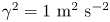 $\gamma ^2=1\ \textrm {m}^{2}\ \textrm {s}^{-2}$ for the model–measurement uncertainty (this is further elaborated in § 6.3.2).
First of all, the streamwise component of the adjoint field is given in figure 2. The field gives a representation of the sensitivity of the cost function to a local perturbation in velocity and the propagated effect through the Navier–Stokes equations. The adjoint field is clearly seen to originate from the lidar measurement locations, due to the forcing term of the adjoint equations being a convolution of the mismatch between the observed and simulated lidar measurements with the lidar filter kernel. The adjoint velocity field propagates upstream due to the reverse sign of the convection term. Note that for a large part of the domain, the adjoint field remains (almost) zero, which indicates that flow information in this region does not influence the measurements. The accuracy of the adjoint gradient is also verified by comparing against a finite-difference evaluation for a few selected perturbation directions. We find that the relative error of the gradient remains smaller than  $0.1\,\%$ for the selected cases. More details are provided in appendix B.
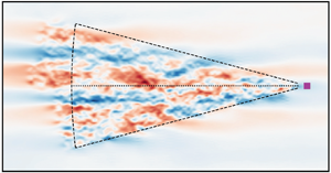
The streamwise component of the adjoint velocity field  $\xi _1$ at
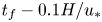 $t_f-0.1H/u_*$
 $(a)$ and
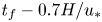 $t_f-0.7H/u_*$
 $(b)$ in an
 $x_1$–
 $x_2$ plane cross-section at
 $x_3=0.1H$. (
 $\blacksquare$, purple): lidar mount location, (
 ): the centre of the range gates, (
 ): the outer edge of the scanning region.

All optimisations are started from an initial guess  $\boldsymbol {a}_0 = \boldsymbol {0}$. The convergence history of the PPI case with
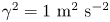 $\gamma ^2=1\ \textrm {m}^2\ \textrm {s}^{-2}$ is shown in figure 3. Figure 3(a) shows the evolution of the cost function as a function of the number of PDE evaluations (LES or adjoint) during the optimisation. For sake of analysis, we split the cost function (see (3.10)) into two parts, i.e.
 $\mathscr {J} = \mathscr {J}_{{b}} + \mathscr {J}_{{o}}$, with
 \begin{equation} \mathscr{J}_{{b}} = \tfrac{1}{2}\|\boldsymbol{a}_0\|^2, \quad \mathscr{J}_{{o}} = \frac{1}{2\gamma^2} \sum_{n=1}^{N_{{m}}} \left\|\boldsymbol{y}_n-\boldsymbol{h}_n(\mathcal{M}_{t}(\boldsymbol{U} + \boldsymbol{\varPsi}\boldsymbol{\varLambda}^{1/2} \boldsymbol{a}_0))\right\|^2. \end{equation}
The first represents the background variability (of the initial condition), and acts as a regularisation term, while the second represents the variability of the observation–model mismatch. Both are shown in the convergence history in figure 3 as well.
 $(a)$ The cost function with (
 $\bullet$, orange):
 $\mathscr {J}_{{o}}$, (
 $\bullet$, green):
 $\mathscr {J}_{{b}}$, (
 $\bullet$, blue):
 $\mathscr {J} = \mathscr {J}_{{o}} + \mathscr {J}_{{b}}$, (
 $\bullet$, black): additional line search iteration.
 $(b)$ Magnitude of the gradient as a function of the number of PDE evaluations.

Each outer optimisation iteration requires a simulation of the forward and adjoint equations, and an additional line search in case the Wolfe conditions are not satisfied (see § 5 for further details). The latter is found to only happen in 15 occasions, so that the number of total PDE simulations (shown in the horizontal axes in figure 3) is to a good approximation twice the number of iterations. Figure 3(b) shows the Euclidean  $(L_2)$ norm of the gradient vector
 $\boldsymbol {\nabla } \mathscr {J}$. Since the optimisation problem is unconstrained, a (local) optimum will correspond to
 $\boldsymbol {\nabla }\mathscr {J}=\boldsymbol {0}$. Given the accuracy of the gradient, which is found to be
 $O(10^{-3})$ (see appendix B), we see that the gradient converges up to a relative value of
 $2\times 10^{-3}$.
An additional point of interest is the computational cost of the reconstruction. All simulations are performed on the Breniac supercomputer of the Flemish supercomputer centre using six computational nodes. Each node consists of two Intel Xeon E5-2680 v4 CPUs and 256 GB of RAM. The nodes are interconnected by an Enhanced Data Rate Infiniband network. The wall times for evaluating the forward and adjoint equations for the LES-based state-space model take respectively 35 s and 55 s, which leads to a total optimisation time of approximately 7.5 h (given 300 iterations).
6.3.2. Tuning of the combined model–measurement uncertainty
In this section the unknown variance  $\gamma ^2$ of the model–measurement mismatch, introduced in § 3.1, is tuned. The regularisation term of the cost function
 $\mathscr {J}_{{b}}$ controls the complexity of the solution, while
 $\gamma ^2 \mathscr {J}_{{o}}$ represents the differences between the simulated and observed measurements. By controlling the parameter
 $\gamma ^2$, the relative trust in the model–measurement accuracy is adjusted. In order to obtain a reasonable value of
 $\gamma ^2$, we solve the optimisation problem (3.10) for a wide range of
 $\gamma ^2$. Note that for each
 $\gamma ^2$, a different optimal initial condition
 $\boldsymbol {u}_0^{\star }$ and as a consequence combination of
 $\gamma ^2 \mathscr {J}_{{o}}^{\star }$ and
 $\mathscr {J}_{{b}}^{\star }$ is obtained. These can be plotted together, i.e.
 $[\gamma ^2 \mathscr {J}_{{o}}^{\star }(\gamma ^2), \mathscr {J}_{{b}}^{\star }(\gamma ^2)]$, and form the so-called Pareto front. Since, this procedure is computationally intensive, we only consider the PPI scanning mode combined with the LES model. In figure 4 the results are shown. It is clearly seen that below
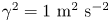 $\gamma ^2=1\ \textrm {m}^{2}\ \textrm {s}^{-2}$ there is almost no decrease in
 $\gamma ^2\mathscr {J}_{{o}}$ while the complexity of the solution increases significantly, which is an indication of overfitting. Therefore we use
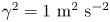 $\gamma ^2=1\ \textrm {m}^{2}\ \textrm {s}^{-2}$. Note that this value is expected to increase when using a lower fidelity model, such as the TFT model and is expected to vary for different scanning modes. Nevertheless, given the relatively low sensitivity of the performance of the reconstruction to this parameter, we also used it for the TFT model and for the Lissajous scanning mode.
Pareto front for the optimisation using the LES model, between the regularisation part of the cost function  $\mathscr {J}_{{b}}$ and the model–observation mismatch
 $\gamma ^2\mathscr {J}_{{o}}$. The annotations at the markers denote different variances
 $\gamma ^2$ of the combined model and measurement uncertainty.

7. Results
7.1. Covariance matrix and POD modes
We start by showing the structure of the covariance tensor. To this end, we visualise the correlation tensor, which is defined as
 \begin{equation} {{\mathsf{C}}_{ij}}(\boldsymbol{x},\breve{\boldsymbol{x}})=\frac{{\mathsf{R}}_{ij}(\boldsymbol{x},\breve{\boldsymbol{x}})}{({\mathsf{R}}_{ii}(\boldsymbol{x},\boldsymbol{x}){\mathsf{R}}_{jj}(\breve{\boldsymbol{x}},\breve{\boldsymbol{x}}))^{1/2}}, \end{equation}
and is an often-used non-dimensionalised version of the covariance tensor (see e.g. Sillero, Jiménez & Moser Reference Sillero, Jiménez and Moser2014; Jiménez Reference Jiménez2018). Figure 5 visualises different cross-sections of the diagonal components ( ${\mathsf{C}}_{11}$,
 ${\mathsf{C}}_{22}$,
 ${\mathsf{C}}_{33}$) of the correlation tensor for reference point
 $\breve {\boldsymbol {x}}=[0,0,L_3/4]$. Figure 5(a–c) visualises
 ${\mathsf{C}}_{11}$, which consists of a central inclined positive lobe laterally surrounded by two negative correlated lobes. The streamwise velocity component of the tensor
 ${\mathsf{C}}_{11}(\boldsymbol {x},\breve {\boldsymbol {x}})$, has been studied in Fang & Porté-Agel (Reference Fang and Porté-Agel2015), but almost exclusively for 1-D streamwise and spanwise variations of
 $\boldsymbol {x}-\breve {\boldsymbol {x}}$. In this work, a similar decay of
 $C_{11}(\boldsymbol {x},\breve {\boldsymbol {x}})$ was found for the streamwise direction of
 ${\mathsf{C}}_{11}(\boldsymbol {x},\boldsymbol {x} \pm 5H\boldsymbol {e}_1)=0.1$. Note that, in this work, additional anti-correlations were observed upstream (between
 $-30H$ and
 $-10H$) and downstream (between
 $10H$ and
 $30H$). However, our domain size is too small to observe this phenomenon. Moreover, an influence of periodic boundary conditions exists and leads to an overestimation of the correlation near the edges of the domain. The correlation of the spanwise velocity component
 ${\mathsf{C}}_{22}$ has a main lobe, which has a steeper inclination angle compared to
 ${\mathsf{C}}_{11}$, and has vertically situated anti-correlated side lobes. Finally, the vertical velocity component correlation
 ${\mathsf{C}}_{33}$ has a relatively narrow main lobe in the spanwise direction. In contrast with the other components, no significant anti-correlated lobes are found.
Visualisation of the two-point correlation  ${\mathsf{C}}_{ij}(\boldsymbol {x},\breve {\boldsymbol {x}})$ with reference point
 $\breve {\boldsymbol {x}}=[0,0,L_3/4]$, (b,e,h) the contour lines of the horizontal
 $x_1$–
 $x_2$ cross-section at
 $x_3=L_3/4$, (a,d,g) the
 $x_1$–
 $x_3$ cross-section at
 $x_2=0$ and (c,f,i) the
 $x_2$–
 $x_3$ cross-section at
 $x_1=0$. Panels (a–c), (d–f) and (g–i) respectively represent the
 ${\mathsf{C}}_{11}$,
 ${\mathsf{C}}_{22}$ and
 ${\mathsf{C}}_{33}$ components. The contour lines are drawn for
 ${\mathsf{C}}_{ij} = [-0.1, -0.05, 0.05, 0.1, 0.3]$. (
 ):
 ${\mathsf{C}}>0$, (
 , red):
 ${\mathsf{C}}<0$.

7.2. Turbulent flow field reconstruction
We now discuss the reconstruction of velocity fields from lidar observations. We first focus on reconstructions using the LES model, and make a qualitative comparison with the solutions from the reference field. Subsequently, a more quantitative error analysis is presented that also includes results of the TFT model (i.e. see figure 10, and related discussion at the end of the current section).
In figure 6, a comparison between the reconstructed velocity fluctuations  $\tilde {\boldsymbol {u}}'$ and the reference velocity fluctuations
 $\boldsymbol {u}'$ is visualised for the PPI lidar scanning mode. Cross-sections of the streamwise velocity are shown at the start (
 $t=t_0$) and end (
 $t=t_f$) of the observation time window. For the horizontal cross-sections (figure 6e–h), in general a good correspondence between
 $\tilde {\boldsymbol {u}}'$ and
 $\boldsymbol {u}'$ is found within the scanned area. We also observe that for the initial and final field, fluctuations in an area upstream and downstream of the scanning region, are also estimated. This is explained by convective transport of flow information out of the measurement area during the measurements. Beyond this convective transport of flow information, additional upstream information is provided due to the relatively long
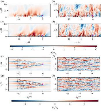
 $u_1$ correlations in streamwise direction. For the vertical cross-section (figure 6a–d), direct flow field observations are only available at
 $z=0.1H$. Due to the lack of mean transport in the vertical direction, additional information is only available due to the regularisation term, and the spatial coherence introduced by the LES model. Nevertheless, it is seen that the large-scale motions are reconstructed in the vertical plane. Since smaller-scale eddies have shorter correlation lengths and turnover times, they are only reconstructed within the scanning region. Outside the scanning region, small-scale turbulent structures are fully decorrelated from the measurements and, therefore, the MAP estimation for these scales will correspond to the maximum of the prior, which is simply zero.
Streamwise component of the velocity field fluctuations in the  $x_2=0$ (a–d) and
 $x_3=0.1H$ (e–h) plane. (a,c,e,g) The reconstructed field
 $\tilde {u}_1$, (b,d,f,h) reference velocity
 $u_1$, (a,b,e,f)
 $t=t_0$, (c,d,g,h):
 $t=t_f$. (
 $\blacksquare$, purple): lidar mount location, (
 ): the centre of the range gates, (
 ): the outer edge of the scanning region.

Figure 7 shows a comparison between reconstructed  $\boldsymbol {h}_n$ and reference
 $\boldsymbol {y}_n$ measurements. We note that the optimisation problem effectively minimises this difference. Thus, as may be expected, the trends are well represented by the reconstructed measurements. We note that the observation operator
 $\boldsymbol {h}_n$ ensures that the reconstructed observations and the reference measurements contain the same scale information. Thus both signals as a function of time for a fixed range gate number (figure 7e–h) transform from relatively smooth close to the sensor location to more irregular further away due to the larger distance covered by the range gate.
Reconstructed  $h_{n,i}$ (
 , blue) and reference
 $y_{n,i}$ (
 , orange) measurements (a–d) for sample numbers
 $n=1$,
 $n= 0.25N_{{s}}$,
 $n= 0.5N_{{s}}$ and
 $n= N_{{s}}$ respectively and (e–h) for range gates
 $i=1$,
 $i= 0.25N_{{r}}$,
 $i= 0.5N_{{r}}$ and
 $i= N_{{r}}$.

Next, we focus on the reconstructed velocity field along lines in the streamwise and spanwise directions, respectively, at time  $t=t_0 + T/4$, at different heights. To this end, figure 8 compares the reconstructed velocity field to the reference field. At this moment, the lidar is in a spanwise extremum position. We first focus on the lines being in the lidar plane. It is observed that the streamwise velocity component
 $u_1$ is well reconstructed, except for the smallest scales. This is expected, since the lidar observations themselves are spatially filtered, while the LES reconstruction mesh is also coarser than the reference (the importance of this effect is further quantified below in figure 10). When looking outside the scanning region, we see a smooth transition to the mean velocity. Looking at the streamwise and wall-normal components, the quality of the reconstruction appears somewhat lower, though the main trends are still recovered. However, when quantifying the errors in more detail (see below), we find that errors in absolute value are of the same order of magnitude for the three components, indicating that the reconstruction is of similar quality for all three directions, even though the lidar only measures along its line of sight, which is dominantly oriented along the
 $u_1$ direction. When comparing the reconstructed and the reference velocity field outside the scanning plane, we observe that the reconstructed field tends more and more to the mean with increasing height, and the error between the two increases consequently. Again, a quantitative evaluation of errors is further addressed in figure 10.
The streamwise (a,b), spanwise (c,d) and wall-normal (e,f) velocity components at  $t = t_i + T/4$. (a,c,e) Along lines in the streamwise direction at different heights
 $h$, i.e.
 $(x_1,0,h)$ with
 $h = [0.1, 0.2,0.4,0.8]H$; (b,d,f) along lines in the spanwise direction
 $8H$ upstream of the mount point, i.e.
 $(-8H,x_2,h)$, at the same set of heights
 $h$. (
 , blue): reconstructed velocity
 $\tilde {\boldsymbol {u}}$, (
 , orange): reference velocity
 $\boldsymbol {u}$.

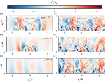
In figure 9 the velocity field reconstruction for the Lissajous scanning mode is shown. Three spanwise–vertical planes are shown at  $t=t_0$ comparing reconstructed to reference velocity field. The dashed line shows the trajectory of the intersect of these planes with the lidar beam during the complete time horizon. The further away the plane is from the lidar mount, the more spatially extended the trajectory becomes in the spanwise and vertical directions. As further quantified below, quality of reconstruction along the height of the boundary layer is a lot better is for this scanning pattern, since direct measurements are available up to
 $0.9H$.
Cross-section at  $x_1 = -10H$ (a,b),
 $x_1 = -5H$ (c,d) and
 $x_1 = 0$ (e,f) of the streamwise component of the velocity field at
 $t=t_0$. (a,c,e) The reconstructed velocity field
 $\tilde {u}_1$, (b,d,f) reference velocity field
 $u_1$, (inline-graphic mime-subtype="png" xlink:href="S0022112020008058_inline530.png"/>): the intersection of the lidar beam with the respective plane for the complete time horizon.

In order to quantify errors in more detail, we define the error on the MAP estimation of the streamwise component as  $\epsilon _1(\boldsymbol {x},t) = I_c^f \circ \tilde {u}_1(\boldsymbol {x},t)-u_{1}(\boldsymbol {x},t)$, where
 $u_{1}$ the fine-grid reference velocity,
 $\tilde {u}_1$ is the reconstructed velocity, and
 $I_c^f$ is a coarse-to-fine interpolation operator, for which we use a combination of linear interpolation in the vertical direction and spectral interpolation (i.e. zero padding in Fourier space) in the horizontal directions. We introduce the error variance averaged over a horizontal region of interest
 $\varGamma$ as
 $\textrm {Var}[\epsilon _1(z,t)] = \langle (\epsilon _1)^2\rangle _{\varGamma }$. To this end, we select a horizontal region that is located inside the lidar observation area. To avoid boundary effects on the error, we omit regions that are less than one convective distance
 $U_{\infty }T$ away from the scanning boundaries, and use
 $\varGamma (z)={\boldsymbol{\mathsf{Q}}}_3({\rm \pi} )[r\cos (\phi ) + U_{\infty } T, r\sin (\phi ) ,z]$ with
 $r\in [r_0 ,r_{{max}}-2U_{\infty } T]$,
 $\phi \in [-\Delta \phi /2, \Delta \phi /2]$ (see also § 6.2). Similar to
 $\textrm {Var}[\epsilon _1(z,t)]$, the error variances for the velocity components in the spanwise and wall-normal directions are also introduced. Finally, since lidars effectively measure a filtered velocity field, we also construct errors based on a filtered reference velocity field. To this end, we filter the fine-grid LES field using a streamwise cutoff filter with
 $k_{{c}} = {\rm \pi}/(\Delta p^2 + \Delta r^2)^{1/2}$, with
 $\Delta p^2= 3/(2\log 2) \Delta p_{1/2}^2$ roughly approximating the lidar filter kernel (2.3).
An overview of the normalised error variance is shown in figure 10 for reconstruction with an LES model, and as point of comparison also for reconstruction with the TFT model. Errors based on unfiltered and filtered reference fields are shown, and results for both the PPI and Lissajous scanning modes are included. As an additional reference, we also show, per component in figure 10, the background variance  $\langle u_{i}^{\prime 2}\rangle _{\varGamma }$, which is the error obtained by predicting with the mean velocity profile. This is the best estimate without or far away from any measurements.
(a,c,e) Normalised error variances as function of height. (b,d,f) Evolution of error variances over the time window, evaluated at height  $z=0.1H$. (a,b) Streamwise velocity component; (c,d) spanwise velocity component; (e,f) vertical velocity component. (blue): reconstruction based on LES; (orange): reconstruction based on TFT; (black): background variance. (
 $\triangle$): PPI scanning mode; (
 $\circ$): Lissajous scanning mode; (
 $\Box$): background variance. (
 ): error with respect to unfiltered reference; (
 ): error with respect to filtered reference.

First of all, it is observed in figure 10 that both scanning trajectories give good results at lidar mount height, though the PPI mode slightly outperforms the Lissajous mode, with a variance of the  $u_{1}$ component that is on average only
 $15\,\%$ of the background variance, compared to
 $25\,\%$ for the Lissajous mode. The best results are obtained in the middle of the assimilation window, and the normalised error variance progressively increases towards the bounds. When looking at higher altitudes, the Lissajous mode clearly outperforms the PPI mode, with an average normalised error variance of
 $25\,\%$ in the region
 $z$ from
 $0.1$ to
 $0.9$, compared to
 $55\,\%$ for the PPI mode. Moreover, in the lidar scanning region, the variance of errors in
 $u_{1}$ is of the same order than those of errors in
 $u_{2}$, and
 $u_{3}$ (in absolute value). This indicates that the estimation distributes the errors evenly in all directions. However, since in boundary layers, the background variance of
 $u'_{1}$ is much larger than that of
 $u'_{2}$, and
 $u'_{3}$, the relative error of the reconstruction in the
 $x_1$ direction is much lower. This explains, the better matching of the
 $u'_{1}$ signal in figure 8 (which is simply larger in amplitude than the other components). Finally, it is also found that LES consistently outperforms TFT, for example for the PPI scanning mode at lidar mount height, the error variance is
 $24\,\%$ an increase by
 $60\,\%$ compared to the LES. The maximum error of the TFT model in the scanning region is
 $35\,\%$, which is an increase by
 $70\,\%$ compared to the LES case.
8. Conclusion
In the current study we investigated reconstructing turbulent flow field from lidar measurements by using a 4D-Var approach in combination with a LES model. The problem was regularised using the background covariance tensor, and reformulated using a POD basis. This allowed the elimination of the continuity constraint, and also led to a better conditioned formulation. Moreover, we used horizontal homogeneity of boundary layers to efficiently construct and represent the POD basis. In order to test the methodology, we constructed virtual lidar measurements from a fine-grid pressure-driven boundary layer, and reconstructed the turbulent flow field using LES on a coarser mesh. This allowed for a detailed error analysis. Different lidar scanning modes were investigated, and a comparison with a TFT model was also included. Overall, LES based reconstruction was quite effective. Inside the general lidar scanning region, we found that errors in the streamwise velocity fluctuation lie between  $15\,\%$ and
 $25\,\%$ (error variance normalised by background variance). Moreover, LES outperformed TFT by 30 %–70 %. In the spanwise and wall-normal directions, the reconstruction quality was the same in absolute value, but worse in relative value, since in turbulent boundary layers the streamwise background variability is substantially higher than spanwise and wall-normal variability.
In the current work, we studied a pressure driven boundary layer as a proxy for a neutral ABL. In reality, effects related to the Ekman spiral (changing wind direction with height), and the capping inversion and free-atmosphere stratification can play an important role in the mean velocity profile. Moreover, near-wall stratification has strong effects on turbulence, requiring the use of correlation tensors that depend on the stratification regime. For homogeneous terrains (offshore, grassland,  $\ldots$), such tensors can be precomputed and parametrised against classical similarity scaling numbers (e.g. based on Richardson number, Rossby number,
 $\ldots$). However, accurate measurements or estimations of the driving conditions (friction velocity, boundary-layer height, Obukhov length,
 $\ldots$) will be necessary for the methodology to work (i.e. for the neutral case, to rescale
 ${{\boldsymbol{\mathsf{R}}}}^+$ to
 ${{\boldsymbol{\mathsf{R}}}}$; see § 3.2). In this context, the effect of bias in the driving conditions on reconstruction efficiency needs to be further investigated. These are important directions for future research.
A further working assumption in the current work, was the use of horizontal homogeneity for the construction of a POD basis in combination with an outer-scaling argument for scaling independent from surface roughness. In reality, effects of inhomogeneity in terrain can have an effect on the outer region of the ABL, and further research needs to investigate whether an imperfect (based on homogeneity assumptions), but efficient POD basis remains effective when terrain features (e.g. wind turbines, buildings) are introduced. Other directions of research may include the use of homogeneous modes, augmented with a relatively small number of non-homogeneous modes to better represent complex terrain. Moreover, the explicit inclusion of model uncertainties (Trémolet Reference Trémolet2006), may also further improve the methodology.
Finally, lidar technology keeps evolving, allowing for faster scans over larger areas. Other sources of measurements with different levels of reliability may also be available, e.g. from drones, met masts, or supervisory control and data acquisition systems in wind farms. Combining these data in a single Bayesian inference framework to optimally reconstruct atmospheric data is an interesting topic for further research. Moreover, some measurement devices such as, e.g. lidar, drones, allow for flexible scanning patterns, that can be optimised to maximise the information obtained from the data, which is also an interesting future research topic.
Declaration of interests
The authors report no conflict of interest.
Appendix A. Derivation and validation of the adjoint gradient
In this appendix, we derive the adjoint equations for the calculation of the gradient of the cost function  $\mathscr {J}(\boldsymbol {a}_0)$ to the control variables
 $\boldsymbol {a}_0$. For the derivation we use a Lagrangian approach (see e.g. Borzi & Schulz Reference Borzi and Schulz2011), similar to the approach by Goit & Meyers (Reference Goit and Meyers2015) to which we refer for further details. To this end, we first reformulate the optimisation problem (3.10) by removing the explicit solution operator
 $\mathcal {M}_{t}$, and instead explicitly adding the state-space constraints, leading to
 \begin{equation} \left. \begin{aligned} \underset{\boldsymbol{a}_0, \tilde{\boldsymbol{u}}, p}{\textrm{minimise}} & \quad \mathcal{J}(\boldsymbol{a}_0, \tilde{\boldsymbol{u}}) = \frac{1}{2}\|\boldsymbol{a}_0\|^2 + \frac{1}{2\gamma^2} \sum_{n=1}^{N_{{m}}} \left\|\boldsymbol{y}_n-\boldsymbol{h}_n\left(\tilde{\boldsymbol{u}}(\boldsymbol{x},t)\right) \right\|^2,\\ \text{subject to} & \quad \frac{ \partial \tilde{\boldsymbol{u}}}{\partial t} +\tilde{\boldsymbol{u}}\boldsymbol{\cdot}\boldsymbol{\nabla} \tilde{\boldsymbol{u}} -u_*^2 H^{-1} \boldsymbol{e}_1+\frac{1}{\rho} \boldsymbol{\nabla} \tilde{p} - \boldsymbol{\nabla}\boldsymbol{\cdot}\boldsymbol{\tau}_{{SGS}} = \boldsymbol{0},\\ & \quad \boldsymbol{\nabla}\boldsymbol{\cdot}\tilde{\boldsymbol{u}} = 0 ,\\ & \quad \tilde{\boldsymbol{u}}(\boldsymbol{x}, t_0)-\boldsymbol{\varPsi}\boldsymbol{\varLambda}^{1/2}\boldsymbol{a}_0 = \boldsymbol{0}. \end{aligned} \right\} \end{equation}
We note that by construction, $\mathscr {J}(\boldsymbol {a}_0)=\mathcal {J}(\boldsymbol {a}_0,\mathcal {M}_{t}(\boldsymbol {u}_0))$. For ease of notation the state variables and the adjoint variables are grouped together and respectively given by
 $\boldsymbol {q}=[\tilde {\boldsymbol {u}}, \tilde {p}]$ and
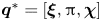 $\boldsymbol {q}^*=[\boldsymbol {\xi },{\rm \pi} , \boldsymbol {\chi }]$. In an analogous way we group together the state-space constraints
 $\boldsymbol {\mathcal {B}}(\boldsymbol {a}_0,\boldsymbol {q})=[\boldsymbol {\mathcal {N}}^{{m}},\boldsymbol {\mathcal {N}}^{{c}},\boldsymbol {\mathcal {C}}]$, which are respectively the momentum, continuity equations and the constraint for the initial condition. The Lagrangian of the above problem is now defined as
 $\mathscr {L}(\boldsymbol {a}_0, \boldsymbol {q},\boldsymbol {q}^*) \triangleq \mathcal {J}(\boldsymbol {a}_0,\boldsymbol {q}) + (\boldsymbol {q}^*,\boldsymbol {\mathcal {B}}(\boldsymbol {a}_0,\boldsymbol {q}))$ and is given by
 \begin{align} \mathscr{L}(\boldsymbol{a}_0, \boldsymbol{q}, \boldsymbol{q}^*) &=\underbrace{\frac{1}{2}\|\boldsymbol{a}_0\|^2 + \frac{1}{2\gamma^2}\sum_{n=1}^{N_{{s}}}\|\boldsymbol{y}_n-\boldsymbol{h}_n(\tilde{\boldsymbol{u}}(\boldsymbol{x},t)) \| }_{\mathcal{J}} \nonumber\\ &\quad + \underbrace{\int_{t_0}^{t_f}\int_{\varOmega}\boldsymbol{\xi}\boldsymbol{\cdot}\left(\frac{ \partial \tilde{\boldsymbol{u}}}{\partial t} +\tilde{\boldsymbol{u}}\boldsymbol{\cdot}\boldsymbol{\nabla} \tilde{\boldsymbol{u}} -u_*^2 H \boldsymbol{e}_1 +\frac{1}{\rho} \boldsymbol{\nabla} \tilde{p} - \boldsymbol{\nabla}\boldsymbol{\cdot}\boldsymbol{\tau}_{{SGS}}\right)\ {\textrm{d}}\boldsymbol{x}{\textrm{d}}t}_{(\boldsymbol{\xi},\boldsymbol{\mathcal{N}}^{{m}})}\nonumber\\ &\quad + \underbrace{\int_{t_0}^{t_f}\int_{\varOmega}{\rm \pi}\left(\boldsymbol{\nabla}\boldsymbol{\cdot}\tilde{\boldsymbol{u}} \right)\, {\textrm{d}}\boldsymbol{x}{\textrm{d}}t}_{({\rm \pi},\boldsymbol{\mathcal{N}}^{{c}})}+\underbrace{\int_{\varOmega} \boldsymbol{\chi}\boldsymbol{\cdot}\left(\tilde{\boldsymbol{u}}(\boldsymbol{x},t_0)-\boldsymbol{\varPsi}\boldsymbol{\varLambda}\boldsymbol{a}_0\right)\, {\textrm{d}}\boldsymbol{x}}_{(\boldsymbol{\chi},\boldsymbol{\mathcal{C}})}. \end{align}
It can be shown (see e.g. Tröltzsch Reference Tröltzsch2010) that, if the adjoint variables are chosen such that  $\mathscr {L}_{\boldsymbol {q}}(\delta \boldsymbol {q}) = 0$ and the state-space constraints
 $\boldsymbol {\mathcal {B}}(\boldsymbol {a}_0,\boldsymbol {q})=\boldsymbol {0}$ are satisfied, then
 $\mathscr {J}_{\boldsymbol {a}_0}(\delta \boldsymbol {a}_0)=\mathscr {L}_{\boldsymbol {a}_0}(\delta \boldsymbol {a}_0)$. Here, we use the Riesz representation theorem to relate gradients to derivatives (see e.g. Borzi & Schulz Reference Borzi and Schulz2011), for example for the cost function this gives
 \begin{equation} \mathscr{J}_{\boldsymbol{a}_0}(\delta \boldsymbol{a}_0) \triangleq\left. \frac{\textrm{d}}{\textrm{d}\alpha}\mathscr{J}(\boldsymbol{a}_0+ \alpha \delta \boldsymbol{a}_0)\right|_{\alpha=0}= \left(\boldsymbol{\nabla} \mathscr{J} , \delta \boldsymbol{a}_0\right). \end{equation}
Further elaborating  $\mathscr {L}_{\boldsymbol {q}}(\delta \boldsymbol {q}) = 0$ gives
 \begin{align} \mathscr{L}_{\boldsymbol{q}}(\delta \boldsymbol{q}) &= \left(\frac{\partial\mathcal{J}}{\partial \tilde{\boldsymbol{u}}},\delta \tilde{\boldsymbol{u}}\right)+\left(\boldsymbol{\xi}, \frac{\partial \boldsymbol{\mathcal{N}}^{{{m}}}}{\partial\tilde{\boldsymbol{u}}}\delta\tilde{\boldsymbol{u}}\right)+\left(\boldsymbol{\xi},\frac{\partial\boldsymbol{\mathcal{N}}^{{{m}}}}{\partial \tilde{p}} \delta\tilde{p}\right) \nonumber\\ &\quad +\left({\rm \pi},\frac{\partial \boldsymbol{\mathcal{N}}^{{{c}}}}{\partial \tilde{\boldsymbol{u}}}\delta\tilde{\boldsymbol{u}}\right)+ \left(\boldsymbol{\chi},\frac{\partial\boldsymbol{\mathcal{C}}}{\partial \tilde{\boldsymbol{u}}}\delta\tilde{\boldsymbol{u}}\right) = 0, \end{align}
where the terms that are trivially zero are left out. Partial integration of the terms  $(\boldsymbol {\xi },[\partial \boldsymbol {\mathcal {N}}^{{m}}/\partial \tilde {\boldsymbol {u}}]\delta \tilde {\boldsymbol {u}})$ and
 $({\rm \pi} ,[\partial \boldsymbol {\mathcal {N}}^{{c}}/\partial {\tilde {\boldsymbol {u}}}]\delta \tilde {\boldsymbol {u}})$, and
 $(\boldsymbol {\xi },[\partial \boldsymbol {\mathcal {N}}^{{{m}}}/\partial \tilde{p}]\delta \tilde {p})$ respectively lead to the unforced adjoint momentum equation and adjoint continuity equation. This is a standard derivation: the result and derivation of the partial integration of the convective terms can be found in Bewley et al. (Reference Bewley, Moin and Temam2001). The terms that are specific to the LES equations, consisting of the subgrid-scale and wall-stress models, are found in Goit & Meyers (Reference Goit and Meyers2015). The remaining non-zero terms will be discussed in the subsequent sections.
A.1. Adjoint contribution of the observations
Linearisation of the cost function to  $\tilde {\boldsymbol {u}}$ gives
 \begin{align}
\left(\frac{\partial\mathcal{J}}{\partial
\tilde{\boldsymbol{u}}},\delta
\tilde{\boldsymbol{u}}\right)
&=\int_{t_0}^{t_f}\int_{\varOmega}\frac{1}{\gamma^2T_{{s}}}\sum_{i=1}^{N_{{r}}}\sum_{n=1}^{N_{{s}}}(y_{n,i}-h_{n,i})
\nonumber\\ &\quad
\times\mathcal{G}_{{l}}\left({\boldsymbol{\mathsf{Q}}}(t)(\boldsymbol{x}-\boldsymbol{x}_{i}(t))\right)\boldsymbol{e}_{{l}}(t)
\, {H}\left(\frac{T_{{s}}}{2}-\big|t -
t_{n-\frac{1}{2}}\big|\right)\boldsymbol{\cdot}\delta
\tilde{\boldsymbol{u}}\,
{\textrm{d}}\boldsymbol{x}{\textrm{d}}t\nonumber\\
&=\left(\sum_{i=1}^{N_{{r}}}\boldsymbol{f}_{i},\delta
\tilde{\boldsymbol{u}}\right),
\end{align}
which leads to the forcing term  $\boldsymbol {f}_i$ for each lidar measurement in the adjoint momentum equations (5.1).
A.2. Adjoint contribution of POD constraints
Linearisation of  $(\boldsymbol {\chi },\boldsymbol {\mathcal {C}})$ to
 $\tilde {\boldsymbol {u}}$ gives
 \begin{equation} \left(\boldsymbol{\chi},\frac{\partial \boldsymbol{\mathcal{C}}}{\partial \tilde{\boldsymbol{u}}}\delta \tilde{\boldsymbol{u}}\right) = \int_{\varOmega} \boldsymbol{\chi}\boldsymbol{\cdot}\delta \tilde{\boldsymbol{u}}(\boldsymbol{x},t_0)\,{\textrm{d}}\boldsymbol{x}.\end{equation}
The only other contribution at  $t_0$ comes from the term
 $[\partial \delta \tilde {\boldsymbol {u}}/\partial t,\boldsymbol {\xi }]$ from the linearised momentum equation, and the combination of both needs to reduce to zero. This can be further elaborated by partial integration
 \begin{equation} \int_{t_0}^{t_f}\int_{\varOmega} \boldsymbol{\xi}\boldsymbol{\cdot}\frac{\partial \delta\tilde{\boldsymbol{u}}}{\partial t}\, {\textrm{d}}{\boldsymbol{x}}{\textrm{d}}t = \left.\int_{\varOmega} \boldsymbol{\xi}\boldsymbol{\cdot} \delta\tilde{\boldsymbol{u}}\, {\textrm{d}}{\boldsymbol{x}}\right|_{t_0}^{t_f}-\int_{t_0}^{t_f}\int_{\varOmega} \frac{\partial \boldsymbol{\xi}}{\partial t}\boldsymbol{\cdot} \delta\tilde{\boldsymbol{u}}\, {\textrm{d}}{\boldsymbol{x}}{\textrm{d}}t. \end{equation}
The second term contributes to the adjoint momentum equations. The first term evaluated at  $t_f$ can be eliminated if
 $\boldsymbol {\xi }(\boldsymbol {x},t_f)=\boldsymbol {0}$ is used as starting condition for the adjoint equations. The first term evaluated at
 $t_0$ combined with (A 6) can be eliminated if
 $\boldsymbol {\chi }(\boldsymbol {x})=\boldsymbol {\xi }(\boldsymbol {x},t_0)$.
A.3. Derivation of the adjoint gradient
The linearisation of the reduced cost function  $\mathscr {J}$ to the control variables
 $\boldsymbol {a}_0$, is given by
 \begin{equation} \mathscr{J}_{\boldsymbol{a}_0}(\delta \boldsymbol{a}_0)=\mathscr{L}_{\boldsymbol{a}_0}(\delta \boldsymbol{a}_0) = \boldsymbol{a}_0 \boldsymbol{\cdot} \delta \boldsymbol{a}_0 - \int_{\varOmega} \boldsymbol{\chi}\boldsymbol{\cdot}\boldsymbol{\varPsi}\boldsymbol{\varLambda}^{1/2}\delta\boldsymbol{a}_0\, \textrm{d}\boldsymbol{x}, \end{equation}
provided that  $\mathscr {L}_{\boldsymbol {q}}(\delta \boldsymbol {q}) = 0$ and
 $\boldsymbol {\mathcal {B}}(\boldsymbol {a}_0,\boldsymbol {q})=\boldsymbol {0}$. The partial derivative to the
 $i$th mode is readily identified as
 $\partial \mathscr {J}/\partial a_{0,i} = a_{0,i} - \lambda _i^{1/2}\int _{\varOmega }\boldsymbol {\xi }(\boldsymbol {x},t_0)\boldsymbol {\cdot }\boldsymbol {\psi }_i \, \textrm {d}\boldsymbol {x}$ (for which
 $\boldsymbol {\chi }(\boldsymbol {x})=\boldsymbol {\xi }(\boldsymbol {x},t_0)$ was also used).
Appendix B. Adjoint gradient validation
In this appendix we compare the adjoint gradient, with finite differences. The finite-difference approximation of the G $\hat{{\rm a}}$teaux derivative is given by
 \begin{equation} \left(\boldsymbol{\nabla} \mathscr{J},\delta \boldsymbol{a}_0\right ) \approx \frac{\mathscr{J}(\boldsymbol{a}_0+\alpha \delta \boldsymbol{a}_0)-\mathscr{J}(\boldsymbol{a}_0)}{\alpha}, \end{equation}
where  $\alpha$ is a factor which controls the step size.
 $\alpha =10^{-6}$ is found as a trade-off between nonlinear effects
 $(\propto \alpha ^2)$ and the finite precision arithmetic by which the calculations are performed, starting to dominate at very small
 $\alpha$. The gradient is validated for both a laminar and turbulent initial velocity field
 $\boldsymbol {u}_0$ of the reconstruction model. Since validating for all the components of the gradient
 $\boldsymbol {\nabla } \mathscr {J}$ would be too time consuming, we use the steepest descent direction
 $\delta \boldsymbol {a}_0 = \boldsymbol {\nabla } \mathscr {J} / \|\boldsymbol {\nabla } \mathscr {J}\|$ obtained from the adjoint approach for the evaluation of the finite-difference method (B 1), and compare results only for this direction.
The results are shown in table 4 for the PPI scanning mode, and are similar for the Lissajous scanning mode. The relative precision for the gradient is around  $10^{-3}$ for the LES and
 $10^{-8}$ for the TFT model. The difference is explained by the differences in spatial discretisation errors, which are significantly larger for the nonlinear terms of the LES, compared to the TFT. Single components of the gradient have also been used, with similar results but are not further reported here.
Comparison of the adjoint and finite-difference gradient, for LES and TFT models, using different initial states; ‘L’ and ‘T’ are respectively abbreviations for laminar and turbulent initial flow conditions.

Appendix C. Interpolation and projection of the two-point covariance tensor
We start by introducing the vertically discretised streamwise velocity vector in Fourier space  $\hat {\boldsymbol {u}}_1(\boldsymbol {k}) = [\hat {u}_1(\boldsymbol {k}, z_1^{{ref}}), \ldots , \hat {u}_1(\boldsymbol {k}, z_{N_{z}^{{ref}}}^{{ref}})]$, with
 $z_i^{{ref}}$ the vertical location of the
 $i$th cell centre. This is repeated for the spanwise and vertical velocities, where the latter component is defined on locations
 ${1}/{2},\ldots , N_z-{1}/{2}$, due to the staggered discretisation in the vertical direction. The velocity can be transformed to physical space by the definition of the Fourier transform
 \begin{equation} \boldsymbol{u}_i(x,y) = \hat{\boldsymbol{u}}_i(\boldsymbol{k})\exp({\textrm{i}}(k_xx+k_yy)), \end{equation}
where  $\boldsymbol {u}_1(x,y) = [u_1(x,y, z_1^{{ref}}), \ldots , u_1(x,y, z_{N_{z}^{{ref}}}^{{ref}})]$ is defined in analogy to
 $\hat {\boldsymbol {u}}_1(\boldsymbol {k})$. We define the discretised two-point covariance matrix on the reference grid as
 \begin{equation} {\boldsymbol{\mathsf{A}}}^{{ref}}(x-\breve{x},y-\breve{y}) = \sum_{|\boldsymbol{k}|\leq\boldsymbol{k}_{{c}}^{{ref}}}\hat{{\boldsymbol{\mathsf{A}}}}^{{ref}}(\boldsymbol{k})\exp({\textrm{i}}(k_x(x-\breve{x})+k_y (y-\breve{y}))), \end{equation}
with
 \begin{align} {\boldsymbol{\mathsf{A}}}^{{ref}}(x-\breve{x},y-\breve{y}) = \begin{bmatrix} {\boldsymbol{\mathsf{A}}}^{{ref}}_{11} & {\boldsymbol{\mathsf{A}}}^{{ref}}_{12} & {\boldsymbol{\mathsf{A}}}^{{ref}}_{13} \\ {\boldsymbol{\mathsf{A}}}^{{ref}}_{21} & {\boldsymbol{\mathsf{A}}}^{{ref}}_{22} & {\boldsymbol{\mathsf{A}}}^{{ref}}_{23} \\ {\boldsymbol{\mathsf{A}}}^{{ref}}_{31} & {\boldsymbol{\mathsf{A}}}^{{ref}}_{32} & {\boldsymbol{\mathsf{A}}}^{{ref}}_{33} \end{bmatrix} \quad \textrm{and} \quad\hat{{\boldsymbol{\mathsf{A}}}}^{{ref}}(\boldsymbol{k}) = \begin{bmatrix} \hat{{\boldsymbol{\mathsf{A}}}}_{11}^{{ref}} & \hat{{\boldsymbol{\mathsf{A}}}}_{12}^{{ref}} & \hat{{\boldsymbol{\mathsf{A}}}}_{13}^{{ref}} \\ \hat{{\boldsymbol{\mathsf{A}}}}_{21}^{{ref}} & \hat{{\boldsymbol{\mathsf{A}}}}_{22}^{{ref}} & \hat{{\boldsymbol{\mathsf{A}}}}_{23}^{{ref}} \\ \hat{{\boldsymbol{\mathsf{A}}}}_{31}^{{ref}} & \hat{{\boldsymbol{\mathsf{A}}}}_{32}^{{ref}} & \hat{{\boldsymbol{\mathsf{A}}}}_{33} ^{{ref}} \end{bmatrix}, \end{align}
where the block matrices  ${\boldsymbol{\mathsf{A}}}^{{ref}}_{qr}(x-\breve {x},y-\breve {y}) = \langle \boldsymbol {u}_q(x,y)\boldsymbol {u}_r^{\intercal }(\breve {x},\breve {y}) \rangle$ and
 $\hat {{\boldsymbol{\mathsf{A}}}}^{{ref}}_{qr}(\boldsymbol {k}) = \langle \hat {\boldsymbol {u}}_q(\boldsymbol {k})\hat {\boldsymbol {u}}_r^*(\boldsymbol {k})\rangle$ (where the superscript
 $*$ denotes the Hermitian transpose) are introduced representing the two-point covariance between the velocity components
 $q$ and
 $r$. It is easily verified that the two-point covariance is by construction symmetric, which translates in Fourier space to
 $\hat {{\boldsymbol{\mathsf{A}}}}^{{ref}}(\boldsymbol {k})=\hat {{\boldsymbol{\mathsf{A}}}}^{{ref},*}(\boldsymbol {k})$, and solenoidal, i.e.
 \begin{equation} \frac{\partial {\boldsymbol{\mathsf{A}}}_{1,j}^{{ref}}}{\partial x} + \frac{\partial {\boldsymbol{\mathsf{A}}}_{2,j}^{{ref}}}{\partial y} + {\boldsymbol{\mathsf{D}}}_z{\boldsymbol{\mathsf{A}}}_{3,j}^{{ref}}=\boldsymbol{0},\quad \textrm{or}\quad \hat{{\boldsymbol{\mathsf{D}}}}^{{ref}}(\boldsymbol{k})\hat{{\boldsymbol{\mathsf{A}}}}^{{ref}}(\boldsymbol{k})=\boldsymbol{0}, \end{equation}
with  ${\boldsymbol{\mathsf{D}}}_z^{{ref}}$ the discrete vertical derivative operator, and
 $\hat {{\boldsymbol{\mathsf{D}}}}^{{ref}}(\boldsymbol {k}) = [\textrm {i}k_x{\boldsymbol{\mathsf{I}}},\textrm {i}k_y{\boldsymbol{\mathsf{I}}},{\boldsymbol{\mathsf{D}}}^{{ref}}_z]$ the divergence operator for mode
 $\boldsymbol {k}$.
The restriction from the reference grid to the optimisation grid, respectively denoted with superscripts ‘ ${ref}$’ and ‘
 ${opt}$’, is now performed in two steps. First, in the horizontal directions, the wavenumbers
 $|\boldsymbol {k}|>\boldsymbol {k}_{{c}}$ are omitted, which is equivalent with a cutoff filter. Second, for the vertical directions, we use linear interpolation. Using
 $\hat {\boldsymbol{\mathsf{B}}}^{{opt}}(\boldsymbol {k})$ to denote the restricted tensor, we use (e.g. elaborated for
 $\hat {\mathsf{B}}_{13}$)
 \begin{equation} \hat{\mathsf{B}}_{13,ij}^{{opt}}(\boldsymbol{k}) = \sum_{m,l} \textrm{tri}\left(\frac{z_i^{{opt}}-z_m^{{ref}}}{\Delta^{{ref}}_3}\right)\textrm{tri}\left(\frac{\breve{z}_{j+1/2}^{{opt}}-\breve{z}_{l+1/2}^{{ref}}}{\Delta^{{ref}}_3}\right)\hat{\mathsf{A}}_{13}^{ml,{ref}}(\boldsymbol{k}), \end{equation}
with  $\textrm {tri}(x) \triangleq \max (1-|x|,0)$ the triangle function, where summation over
 $m,l$ corresponds to summation over all vertical locations on the reference grid.
However, the interpolated covariance operator is in general not solenoidal, i.e. 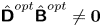 $\hat {{\boldsymbol{\mathsf{D}}}}^{{opt}}\hat {\boldsymbol{\mathsf{B}}}^{{opt}}\ne \boldsymbol {0}$. To resolve this, we start by defining the Hilbert–Schmidt norm of the two-point covariance tensor
 \begin{align} \|{\boldsymbol{\mathsf{A}}}\|^2 &= \frac{1}{L_x^2L_y^2}\int_{0}^{L_x}\int_{0}^{L_x}\int_{0}^{L_y}\int_{0}^{L_y} \left\|\sum_{|\boldsymbol{k}|\leq\boldsymbol{k}_{{c}}}\hat{{\boldsymbol{\mathsf{A}}}}(\boldsymbol{k})\exp(\textrm{i}(k_x(x-\breve{x})+k_y (y-\breve{y}))\right\|^2 \, {\textrm{d}}x{\textrm{d}}\breve{x}{\textrm{d}}y{\textrm{d}}\breve{y} \nonumber\\ \quad &= \sum_{|\boldsymbol{k}|\leq\boldsymbol{k}_{{c}}}\|\hat{{\boldsymbol{\mathsf{A}}}}(\boldsymbol{k})\|^2 = \sum_{|\boldsymbol{k}|\leq\boldsymbol{k}_{{c}}}\hat{\mathsf{A}}_{ij}(\boldsymbol{k})\hat{\mathsf{A}}^*_{ij}(\boldsymbol{k}), \end{align}
which is a direct consequence of Parseval's theorem. The closest two-point covariance tensor  ${\boldsymbol{\mathsf{A}}}^{{opt}}$, that is conjugate symmetric and solenoidal on the optimisation grid (
 ${\boldsymbol{\mathsf{A}}}^{{opt}}$) can then be found as
 \begin{align} \left. \begin{aligned} \underset{\hat{{\boldsymbol{\mathsf{A}}}}^{{opt}}}{\text{minimise}} & \quad \sum_{|\boldsymbol{k}|\leq\boldsymbol{k}_{{c}}^{{opt}}}\tfrac{1}{2}\|\hat{{\boldsymbol{\mathsf{A}}}}^{{opt}}(\boldsymbol{k}) - \hat{\boldsymbol{\mathsf{B}}}^{{opt}}(\boldsymbol{k})\|^2,\\ \text{subject to} & \quad \hat{\mathsf{D}}^{{opt}}_{ik}(\boldsymbol{k})\hat{\mathsf{A}}^{{opt}}_{kj}(\boldsymbol{k}) = 0,\ \ \hat{\mathsf{A}}^{{opt}}_{ij}(\boldsymbol{k}) = \hat{\mathsf{A}}_{ji}^{{opt},*}(\boldsymbol{k}), \quad \hat{\mathsf{A}}^{{opt}}_{ij}(\boldsymbol{k}) = \hat{\mathsf{A}}^{{opt},*}_{ij}(-\boldsymbol{k}) \quad\forall i,j,\boldsymbol{k}, \end{aligned} \right\} \end{align}
where the last constraint enforces  $\hat {{\boldsymbol{\mathsf{A}}}}^{{opt}}$ to be strictly real. Since,
 $\hat {\mathsf{A}}^{{opt}}_{ij}(\boldsymbol {k}) = \hat {\mathsf{A}}^{{opt},*}_{ij}(-\boldsymbol {k})$, only half of the wavenumbers need to be considered. The contributions of the remaining wavenumbers are independent, and therefore the optimisation can be performed per wavenumber
 $\boldsymbol {k}$.
To continue, for notational simplicity the explicit  $\boldsymbol {k}$ dependence of the matrices, and the ‘
 ${opt}$’ superscript are further omitted. In order to find the optimum, we construct the Lagrangian
 \begin{align} \mathcal{\mathscr{L}} &= \tfrac{1}{2}(\hat{\mathsf{A}}_{ij} - \hat{\mathsf{B}}_{ij})(\hat{\mathsf{A}}_{ij}^* - \hat{\mathsf{B}}_{ij}^*) + \textrm{Re}(\varLambda_{kj})\textrm{Re}(\hat{\mathsf{D}}_{ki}\hat{\mathsf{A}}_{ij})-\textrm{Im}(\varLambda_{kj})\textrm{Im}(\hat{\mathsf{D}}_{ki}\hat{\mathsf{A}}_{ij}) \nonumber\\ &\quad + \textrm{Re}({\varGamma}_{ij})\textrm{Re}(\hat{\mathsf{A}}_{ij}-\hat{\mathsf{A}}_{ji}^*) - \textrm{Im}({\varGamma}_{ij})\textrm{Im}(\hat{\mathsf{A}}_{ij}-\hat{\mathsf{A}}_{ji}^*), \end{align}
where  $\varLambda _{ij}$ and
 $\varGamma _{ij}$ are respectively the Lagrangian multipliers for the divergence and conjugate symmetry constraint. We note that, the sign of the complex constraints can be freely chosen; the minus sign will be convenient for further notation. Since (C 7) is a quadratic program, a sufficient condition for optimality is given by
 \begin{gather} \frac{\partial \mathscr{L}}{\partial \textrm{Re}( \hat{\mathsf{A}}_{ij})} = \textrm{Re}(\hat{\mathsf{A}}_{ij} - \hat{\mathsf{B}}_{ij} + \varLambda_{kj}\hat{\mathsf{D}}_{ki} + \varGamma_{ij}-\varGamma_{ji}) = 0, \end{gather}
 \begin{gather}\frac{\partial \mathscr{L}}{\partial \textrm{Im}( \hat{\mathsf{A}}_{ij})} = \textrm{Im}(\hat{\mathsf{A}}_{ij} - \hat{\mathsf{B}}_{ij} - \varLambda_{kj}\hat{\mathsf{D}}_{ki} + \varGamma_{ij}-\varGamma_{ji}^*) = 0, \end{gather}
or equivalently in matrix form
 \begin{equation} \hat{{\boldsymbol{\mathsf{A}}}} - \hat{\boldsymbol{\mathsf{B}}} + \hat{{\boldsymbol{\mathsf{D}}}}^*\boldsymbol{\varLambda} + \boldsymbol{\varGamma}-\boldsymbol{\varGamma}^* = \boldsymbol{0}. \end{equation}
The values of the Lagrange multipliers are found by enforcing the constraints. By using the conjugate symmetry,  $\hat {{\boldsymbol{\mathsf{A}}}} = \hat {{\boldsymbol{\mathsf{A}}}}^*$, we find an expression for
 $\boldsymbol {\varGamma } - \boldsymbol{\varGamma}^*$,
 \begin{equation} \boldsymbol{\varGamma} - \boldsymbol{\varGamma}^* = \tfrac{1}{2}(\hat{\boldsymbol{\mathsf{B}}}- \hat{\boldsymbol{\mathsf{B}}}^* + \boldsymbol{\varLambda}^*\hat{{\boldsymbol{\mathsf{D}}}} -\hat{{\boldsymbol{\mathsf{D}}}}^*\boldsymbol{\varLambda}). \end{equation}
Subsequently substituting into (C 11), gives
 \begin{equation} \hat{{\boldsymbol{\mathsf{A}}}}-\hat{\boldsymbol{\mathsf{B}}}- \tfrac{1}{2}(\hat{\boldsymbol{\mathsf{B}}}+\hat{\boldsymbol{\mathsf{B}}}^*) + \tfrac{1}{2}(\boldsymbol{\varLambda}^*\hat{{\boldsymbol{\mathsf{D}}}} +\hat{{\boldsymbol{\mathsf{D}}}}^*\boldsymbol{\varLambda}) = 0. \end{equation}
Using the continuity equation  $\hat {{\boldsymbol{\mathsf{D}}}}\hat {{\boldsymbol{\mathsf{A}}}}=0$ in (C 13), and some additional tedious but straightforward algebraic manipulations, we further find
 \begin{equation} \boldsymbol{\varLambda}^*\hat{{\boldsymbol{\mathsf{D}}}} +\hat{{\boldsymbol{\mathsf{D}}}}^*\boldsymbol{\varLambda} = \tfrac{1}{2}(\hat{\boldsymbol{\mathsf{B}}}+\hat{\boldsymbol{\mathsf{B}}}^*) - \tfrac{1}{2}({\boldsymbol{\mathsf{I}}}-\hat{{\boldsymbol{\mathsf{D}}}}^*(\hat{{\boldsymbol{\mathsf{D}}}}\hat{{\boldsymbol{\mathsf{D}}}}^*)^{-1}\hat{{\boldsymbol{\mathsf{D}}}})(\hat{\boldsymbol{\mathsf{B}}}+\hat{\boldsymbol{\mathsf{B}}}^*)({\boldsymbol{\mathsf{I}}}-\hat{{\boldsymbol{\mathsf{D}}}}(\hat{{\boldsymbol{\mathsf{D}}}}\hat{{\boldsymbol{\mathsf{D}}}}^*)^{-1}\hat{{\boldsymbol{\mathsf{D}}}}^{*}). \end{equation}
Inserting (C 14) in (C 13) finally leads to an expression for  $\hat {{\boldsymbol{\mathsf{A}}}}$,
 \begin{equation} \hat{{\boldsymbol{\mathsf{A}}}} = \tfrac{1}{2}({\boldsymbol{\mathsf{I}}}-\hat{{\boldsymbol{\mathsf{D}}}}^*(\hat{{\boldsymbol{\mathsf{D}}}}\hat{{\boldsymbol{\mathsf{D}}}}^*)^{-1}\hat{{\boldsymbol{\mathsf{D}}}})(\hat{\boldsymbol{\mathsf{B}}}+\hat{\boldsymbol{\mathsf{B}}}^*)({\boldsymbol{\mathsf{I}}}-\hat{{\boldsymbol{\mathsf{D}}}}(\hat{{\boldsymbol{\mathsf{D}}}}\hat{{\boldsymbol{\mathsf{D}}}}^*)^{-1}\hat{{\boldsymbol{\mathsf{D}}}}^{*}). \end{equation}
Here, the operator  ${\boldsymbol{\mathsf{I}}}-\hat {{\boldsymbol{\mathsf{D}}}}^*(\hat {{\boldsymbol{\mathsf{D}}}}\hat {{\boldsymbol{\mathsf{D}}}}^*)^{-1}\hat {{\boldsymbol{\mathsf{D}}}}$ represents the orthogonal projection on the solenoidal space.
The left and right projections on the solenoidal space are in practice computed sequentially. The left projection  $\hat {\boldsymbol{\mathsf{L}}}\triangleq ({\boldsymbol{\mathsf{I}}}-\hat {{\boldsymbol{\mathsf{D}}}}^*(\hat {{\boldsymbol{\mathsf{D}}}}\hat {{\boldsymbol{\mathsf{D}}}}^*)^{-1}\hat {{\boldsymbol{\mathsf{D}}}})(\hat {\boldsymbol{\mathsf{B}}}+\hat {\boldsymbol{\mathsf{B}}}^*)/2$, for example, can be found by first solving
 \begin{equation} -\hat{{\boldsymbol{\mathsf{D}}}}\hat{{\boldsymbol{\mathsf{D}}}}^*{\boldsymbol{\mathsf{X}}} = -\tfrac{1}{2}\hat{{\boldsymbol{\mathsf{D}}}}(\hat{\boldsymbol{\mathsf{B}}}+\hat{\boldsymbol{\mathsf{B}}}^*), \end{equation}
for  ${\boldsymbol{\mathsf{X}}}$, where
 $-\hat {{\boldsymbol{\mathsf{D}}}}^*$ is the definition of the discrete gradient, such that
 $-\hat {{\boldsymbol{\mathsf{D}}}}\hat {{\boldsymbol{\mathsf{D}}}}^* = -(k_x^2+k_y^2) {\boldsymbol{\mathsf{I}}} - {\boldsymbol{\mathsf{D}}}_z{\boldsymbol{\mathsf{D}}}_z^*$ is the definition of a discrete Laplacian (see Verstappen & Veldman (Reference Verstappen and Veldman2003) for further details), and
 ${\boldsymbol{\mathsf{X}}}$ is a potential. Note that this procedure is similar to the one for obtaining the pressure gradient with a pressure-correction approach. The left projected part of the two-point covariance is then given by
 \begin{equation} \hat{\boldsymbol{\mathsf{L}}}\triangleq \tfrac{1}{2}({\boldsymbol{\mathsf{I}}}-\hat{{\boldsymbol{\mathsf{D}}}}^*(\hat{{\boldsymbol{\mathsf{D}}}}\hat{{\boldsymbol{\mathsf{D}}}}^*)^{-1}\hat{{\boldsymbol{\mathsf{D}}}})(\hat{\boldsymbol{\mathsf{B}}}+\hat{\boldsymbol{\mathsf{B}}}^*) = \tfrac{1}{2}(\hat{\boldsymbol{\mathsf{B}}}+\hat{\boldsymbol{\mathsf{B}}}^*) - \hat{{\boldsymbol{\mathsf{D}}}}^*\boldsymbol{X}. \end{equation}
The right projection  $\hat {{\boldsymbol{\mathsf{A}}}} = \hat {\boldsymbol{\mathsf{L}}} ({\boldsymbol{\mathsf{I}}}-\hat {{\boldsymbol{\mathsf{D}}}}(\hat {{\boldsymbol{\mathsf{D}}}}\hat {{\boldsymbol{\mathsf{D}}}}^*)^{-1}\hat {{\boldsymbol{\mathsf{D}}}}^{*})$ is computed afterwards in completely analogous way.