1. Introduction
Vortices abound in the oceans and have horizontal scales from 1 to 250 km; below 10 km radius (at midlatitudes), the vortices are called submesoscale; above, they are mesoscale vortices. Mesoscale vortices have been estimated to contribute to half of the transport in the oceans according to the recent analysis by Zhang, Wang & Qiu (Reference Zhang, Wang and Qiu2014). Earlier estimates of the vortex population in the surface layers of the North Atlantic indicate the presence of around 1000 to 10 000 structures, see Ebbesmeyer et al. (Reference Ebbesmeyer, Taft, McWilliams, Shen, Riser, Rossby, Biscaye and Östlund1986). These vortices, which are often long-lived, carry momentum, energy, salinity and heat over long distances across the oceans. Isolated vortices do not self-advect, but they can drift via mutual interactions or via interactions with other dynamical structures or environmental elements (mean flows, jet flows, vertically sheared currents, bottom topography, Earth curvature, marine boundaries).
Vortex interactions have been extensively studied in the literature. One efficient motion-inducing vortex interaction has been identified by Gryanik (Reference Gryanik1983a
) and Hogg & Stommel (Reference Hogg and Stommel1985) in the context of a two-layer model. It consists of a baroclinic pair of opposite sign vortices, placed in different layers. Hogg & Stommel (Reference Hogg and Stommel1985) named such structures ‘hetons’ due to their ability to carry heat across the oceans. Hetons have since been the topic of many studies, mostly in few-layer models. A review may be found in the textbook by Sokolovskiy & Verron (Reference Sokolovskiy and Verron2014). Previous works have included the study of singularities in two-layer (Gryanik Reference Gryanik1983a
; Young Reference Young1985) or
 $N$
-layer models (Gryanik & Tevs Reference Gryanik and Tevs1989) and continuous stratification (Gryanik Reference Gryanik1983b
). Experimental studies were also conducted by, e.g., Griffith & Hopfinger (Reference Griffith and Hopfinger1986). The stability of finite-core hetons has been addressed by Flierl (Reference Flierl1988) in the two-layer model. The stability of hetons has also been studied in the case where the poles are separated in the vertical; see Reinaud & Carton (Reference Reinaud and Carton2009) for vertically aligned poles and more recently Reinaud (Reference Reinaud2015) for horizontally offset poles. Hetons were also observed in situ in the Gulf of Cadiz by Carton et al. (Reference Carton, Chérubin, Paillet, Morel, Serpette and Le Cann2002).
A heton may also interact with another potential vorticity (PV) structure, and in particular with another heton. The interaction between hetons was indeed observed by L’Hegaret et al. (Reference L’Hegaret, Carton, Ambar, Menesguen, Hua, Chérubin, Aguiar, Le Cann, Daniault and Serra2014), again in the Gulf of Cadiz. In this case, the interaction between two hetons initially resulted in the formation of a baroclinic tripolar vortex. Although the tripole eventually breaks due to the
 ${\it\beta}$
-effect, the study of its formation is of relevance to the present study. Interactions between hetons have also been investigated numerically in two-layer models by Sokolovskiy & Carton (Reference Sokolovskiy and Carton2010), and the head-on collision of hetons in continuously stratified fluid has been investigated by Reinaud & Carton (Reference Reinaud and Carton2015). It should be noted that the interaction between two singular hetons (referred to as hetonic quartets) has been studied in two layers including on the
 ${\it\beta}$
-plane by Kizner (Reference Kizner2006). All of these interactions may produce multipolar vortices as either the product of baroclinic instabilities and/or the merger of like-signed poles or destructive interaction between horizontally aligned dipoles. A possible outcome of the interaction between hetons is the formation of tripolar structures, and this is the focus of the present study. Such structures may be formed in the case of two hetons colliding while being slightly offset in the horizontal direction. In these situations, two of the poles at the same depth may come very close to one another and merge. The two other vortices lying at different depths will remain distant from one another and therefore will not merge. An important feature of the resulting structure is that it may be stationary (albeit rotating on itself), in particular if the original hetons carry opposite linear momentum. In this sense, the interaction halts the transport. However, the tripolar structure formed from the interaction may be unstable and break back into new hetons which would resume a translating motion and further transport their associated properties. Hence, the stability of tripolar structures as well as their formation process are important dynamical events which need to be better understood.
Tripolar structures have been studied in the context of a two-layer flow, using singularities, by Sokolovskiy, Koshel & Verron (Reference Sokolovskiy, Koshel and Verron2013) and Koshel, Sokolovskiy & Verron (Reference Koshel, Sokolovskiy and Verron2013), and, more recently, the equilibria of finite-core tripoles has been investigated by Shteinbuch-Fridman et al. (Reference Shteinbuch-Fridman, Makarov, Carton and Kizner2015). The set-up of our experiments differs from that of earlier studies in several aspects. First, our model describes a continuously stratified fluid, and not a two-layer fluid. Second, the geometry of our problem has two main differences from previous cases. The first difference is the existence of a layer of fluid, with zero potential vorticity, separating the poles of the tripoles vertically, whereas in Shteinbuch-Fridman et al. (Reference Shteinbuch-Fridman, Makarov, Carton and Kizner2015), the two layers containing the vortices are adjacent. The second difference lies in the aspect ratio of the poles which affects their sensitivity to baroclinic modes of perturbation. Indeed, vortices with large width-to-height aspect ratios are more prone to baroclinic instability.
The paper is organised as follows. Section 2 reviews the governing equation of motion. Section 3 considers the stability of a triplet of point vortices in the configuration of interest. In this configuration the point vortices are horizontally aligned and this alignment can only be broken by nonlinear effects. We next consider the existence and stability of finite-core baroclinic tripoles at equilibrium. Instability modes associated with the deformation of the finite-core vortices may be triggered, and it is shown that these tripoles may indeed be sensitive to baroclinic instability modes. This is further illustrated by investigation of the nonlinear evolution of tripoles initially consisting of three cylindrical vortices. Finally, the formation of such tripoles from the collision of offset hetons is shown. This formation is a common occurrence provided that the horizontal position of the poles is suitable, i.e. when two poles face each another. Conclusions are drawn in the last section, while technical details are provided in appendices A–D.
2. Equations of motion
We consider flows under the quasi-geostrophic approximation, valid for oceanic vortex flows with moderate velocities. This approximation stems from a first-order expansion of the primitive equations in Rossby number. This approximation is strictly valid for
 $Fr^{2}\ll Ro\ll 1$
. Here,
 $Fr=U/(NH)$
is the Froude number, the ratio of a horizontal vorticity
 $U/H$
to the buoyancy, or Brunt–Väisälä, frequency
 $N$
of the stably stratified fluid;
 $U$
is a typical horizontal velocity scale and
 $H$
is a vertical length scale. The Rossby number is defined as the ratio
 $Ro=U/(fL)$
, where
 $L$
is a horizontal length; hence,
 $U/L$
scales as the vertical component of vorticity, also called relative vorticity;
 $f$
is the Coriolis frequency, or background planetary vorticity, associated with the rotation of the planet. For the sake of simplicity, we assume that both
 $N$
and
 $f$
are constant. In that case, one can define a stretched vertical coordinate
 $z$
from the actual local depth
 $z^{\ast }$
by
 $z=Nz^{\ast }/f$
. It should be noted that, in practice, the ratio
 $N/f$
is typically large at midlatitude. In this new reference frame the streamfunction
 ${\it\psi}$
of the horizontal advecting velocity field can be deduced from the spatial distribution of the key prognostic variable, the potential vorticity anomaly
 $q$
, from a linear and isotropic relation, a Poisson equation that reads
 $$\begin{eqnarray}{\rm\Delta}{\it\psi}=q.\end{eqnarray}$$
It should be noted that if the advecting velocity field has only two non-zero components
 $\boldsymbol{u}=(u,v,0)$
with
 $$\begin{eqnarray}u=-\frac{\partial {\it\psi}}{\partial y}\quad \text{and}\quad v=\frac{\partial {\it\psi}}{\partial x},\end{eqnarray}$$
all fields,
 $q$
,
 ${\it\psi}$
and
 $\boldsymbol{u}$
depend on the three spatial coordinates
 $(x,y,z)$
, and on time, and the Laplace operator of the Poisson equation is the three-dimensional operator
 ${\rm\Delta}=\partial ^{2}/\partial x^{2}+\partial ^{2}/\partial y^{2}+\partial ^{2}/\partial z^{2}$
. The last equation that closes the system relates to the material conservation of the potential vorticity, which reads (on the
 $f$
-plane)
 $$\begin{eqnarray}\frac{\text{D}q}{\text{D}t}=0,\end{eqnarray}$$
where
 $\text{D}/\text{D}t=\partial /\partial t+\boldsymbol{u}\boldsymbol{\cdot }\boldsymbol{{\rm\nabla}}=\partial /\partial t+J({\it\psi},\cdot )$
is the material derivative. It should be noted that the nonlinearity of the quasi-geostrophic system occurs only in this advection equation. For the full derivation, see, e.g., Vallis (Reference Vallis2006).
3. Structure and stability of baroclinic tripoles
We first analyse the structure and stability of baroclinic tripolar vortices which may emerge from the nonlinear interaction of two hetons. These tripoles can be referred to as
 ${\it\Lambda}$
-tripoles or as carrousel tripoles due to their shape (Sokolovskiy & Carton Reference Sokolovskiy and Carton2010). The formation of such tripoles from the collision of two hetons will be discussed in the following section; here, we assume that the like-signed poles of the two hetons, lying near the surface, have already merged and that their combination now consists of a single pole. We determine the equilibria of these tripoles and address their stability.
3.1. Point vortex approximation
Here, the
 ${\it\Lambda}$
-tripole is idealised as a triplet of point vortices. The three-point vortex problem has been studied in detail in a two-layer model by Sokolovskiy et al. (Reference Sokolovskiy, Koshel and Verron2013) and Koshel et al. (Reference Koshel, Sokolovskiy and Verron2013). They showed that chaotic advection is possible if symmetry is lost. This case will not be considered here. Point vortex triplet equilibria are composed of two equal strength vortices (the satellites), a distance apart, at the same depth, and of another vortex (of opposite and double strength), above them, and on the rotation axis of the initial pair (we call it the core vortex). By symmetry, the core vortex does not move and the satellites rotate around it at the same rate.
We denote by
 ${\it\kappa}_{i},i=1,2,3$
, the strength of the vortex located at
 $\boldsymbol{x}_{i}$
rescaled by
 $4{\rm\pi}$
. For an equivalent finite-core vortex, we would have
 $$\begin{eqnarray}{\it\kappa}_{i}=\frac{1}{4{\rm\pi}}\iiint _{V_{i}}q\,\text{d}v,\end{eqnarray}$$
where
 $V_{i}$
is the volume of PV of the vortex
 $i$
. For singular vortices,
 ${\it\kappa}$
is the strength associated with the Dirac distribution divided by
 $4{\rm\pi}$
.
Thus, vortex 1 of strength
 ${\it\kappa}_{1}=-{\it\kappa}$
is located at
 $\boldsymbol{x}_{1}=(-x_{0},0,0)$
; vortex 2 has
 ${\it\kappa}_{2}=2{\it\kappa}$
, and lies at
 $\boldsymbol{x}_{2}=(0,0,z_{0})$
, and vortex 3 has
 ${\it\kappa}_{3}=-{\it\kappa}$
, and is at
 $\boldsymbol{x}_{3}=(x_{0},0,0)$
.
The rotation rate of the point vortex triplet is
 $$\begin{eqnarray}{\it\Omega}=2{\it\kappa}\left({\displaystyle \frac{1}{(x_{0}^{2}+z_{0}^{2})^{3/2}}}-\frac{1}{8x_{0}^{3}}\right).\end{eqnarray}$$
We now add perturbations to the location of the point vortices (the perturbations have the form
 $(x_{i}^{\prime },y_{i}^{\prime })=(\tilde{x_{i}^{\prime }},\tilde{y_{i}^{\prime }})\text{e}^{b{\it\lambda}t}$
, where
 $\tilde{x_{i}^{\prime }}$
and
 $\tilde{y_{i}^{\prime }}$
are time-independent,
 $b$
is the relevant time scale defined below). It should be noted that we do not consider perturbations in the
 $z$
-direction. This is due to the lack of vertical advection in quasi-geostrophic dynamics. The
 $z$
-location of a singularity is time-independent. We derive the linearised equations of motion for the perturbations, in the frame of reference rotating at
 ${\it\Omega}$
; we solve the associated eigenvalue problem.
The details of the calculation are given in appendix A.
The outcome is that the configuration is neutrally stable as the six non-dimensional eigenvalues
 ${\it\lambda}$
are
 $$\begin{eqnarray}\displaystyle & {\it\lambda}=0,0, & \displaystyle\end{eqnarray}$$
 $$\begin{eqnarray}\displaystyle & -\text{i}((2a)^{3}-1)/4,\quad -\text{i}((2a)^{3}-1)/4, & \displaystyle\end{eqnarray}$$
 $$\begin{eqnarray}\displaystyle & \text{i}((2a)^{3}-1)/4,\quad \text{i}((2a)^{3}-1)/4, & \displaystyle\end{eqnarray}$$
 $$\begin{eqnarray}\displaystyle & b={\it\kappa}/x_{0}^{3}, & \displaystyle\end{eqnarray}$$
 $$\begin{eqnarray}\displaystyle & a=(1+(z_{0}/x_{0})^{2})^{-1/2}. & \displaystyle\end{eqnarray}$$
 ${\it\lambda}=0$
, and
 ${\it\lambda}=\pm A$
, where
 $A=\text{i}((2a)^{3}-1)/4=\text{i}{\it\Omega}/b$
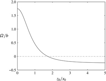
, a steady perturbation and two frequencies for oscillatory modes (imaginary numbers). It should be noted that this means that an infinitesimal perturbation does not make the system of point vortices rapidly move away from its equilibrium position and the situation is robust. This is due to the symmetry of the tripole and to the linearity of the dynamics. The non-dimensional rotation rate
 ${\it\Omega}/b=2({\it\alpha}^{3}-1/8)$
, which also corresponds to the non-dimensional non-zero frequencies
 $A$
, is plotted versus the relative vertical to horizontal distance
 $z_{0}/x_{0}$
in figure 1. It should be noted that it changes sign when
 $a=0.5$
, i.e.
 $z_{0}/x_{0}=\sqrt{3}$
. For
 $z_{0}/x_{0}<\sqrt{3}$
the central vortex (with positive rotation) dominates the overall rotation. As
 $z_{0}/x_{0}$
is taken further up, the global rotation becomes dominated by the negative rotation of the bottom satellites.
Non-dimensional rotation rate
 ${\it\Omega}$
(solid line) for the singular
 ${\it\Lambda}$
-tripole versus the relative vertical to horizontal separation of the poles
 $z_{0}/x_{0}$
. The dash-dotted line indicates
 ${\it\Omega}/b=0$
.

3.2. Finite-core equilibria
The fact that the point vortex triplet shows no instability does not imply that finite-core
 ${\it\Lambda}$
-tripoles are stable. Indeed, other modes of instability related to the deformation of the finite-area vortices may then emerge. One other way to see the problem is to consider the continuous distributions of PV that represent the finite-core poles as infinite (continuous) distributions of point vortices;
 $N>3$
point vortices may exhibit chaotic behaviour which is seen as an instability in the continuous set-up.
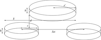
By analogy with the point vortex triplet, in the finite-core vortices, the poles with negative PV,
 $-q$
, (the satellites) are located below and are separated by a distance
 ${\rm\Delta}x$
(see figure 2). They have radius
 $r$
, and hence a strength of
 $-{\it\kappa}=-qV/(4{\rm\pi})=-qr^{2}h/4$
. The positive pole (the core) is placed on the axis of rotation of the pair and is offset in the vertical by a layer with no PV of thickness
 $d$
. Its strength is twice the strength of the satellites, and is opposite-signed, ensuring that the structure has an overall zero strength. All poles have the same height
 $h$
. The radius of the core is set to
 $r^{\prime }=\sqrt{2}r$
so that its PV is equal and opposite to that of the satellites. Although results will be presented with non-dimensional parameters, all calculations are carried out setting the height of the three poles to unity for the equilibria. Hence, variation of
 $r$
or the aspect ratio
 $r/h$
is identical in practice.
Structure and geometric parameters for the finite-core hetons. Here,
 $h$
is the height of the hetons,
 $r$
is the mean horizontal radius of the side poles, while
 $r^{\prime }=\sqrt{2}r$
is the mean horizontal radius of the central pole;
 $d$
is the vertical gap with no PV between the poles – two lower side poles and the upper central pole;
 ${\rm\Delta}x$
is the horizontal separation distance between the side pole centres;
 ${\it\delta}$
is the horizontal separation distance between the left outermost edge of the side vortex and the right outermost edge of the central vortex.

First, we calculate equilibrium states for the
 ${\it\Lambda}$
-vortices. In practice, the states are obtained numerically. The vertical direction is discretised by a large number of horizontal ‘layers’. We typically discretise each pole by at least
 $n_{c}=25$
horizontal layers. As mentioned in appendix B, due to the choice of PV, we restrain our study to symmetric configurations. We perform two cross-sections in the parameter space
 $(r/h,d/h)$
. It should be noted that for practical reasons
 $d/h$
is taken as a fraction of the number of layers
 $n_{c}$
mapping each vortex. Hence, it is taken as a fraction of the form
 $d/h=n_{d}/n_{c}$
, where
 $n_{d}$
is the number of empty layers between the lower poles and the upper (central) pole. It should be noted also that the aspect ratio for the central vortex
 $r^{\prime }/h\equiv \sqrt{2}r/h$
. As a consequence, hereafter we only refer to the aspect ratio
 $r/h$
, the aspect ratio of the satellites. The aspect ratio for the core vortex is then implicitly defined by
 $r^{\prime }/h$
and is omitted in the text.
The first cross-section focuses on the influence of the aspect ratio
 $r/h$
and corresponds to
 $d/h=1$
, while
 $2\leqslant r/h\leqslant 8$
with an increment of 0.5 between cases. The second cross-section focuses on the influence of the vertical offset. It corresponds to a fixed aspect ratio
 $r/h=3$
for the side vortex and varying
 $d/h=0$
, 0.12, 0.24, 0.52, 1, 1.52 and 2.
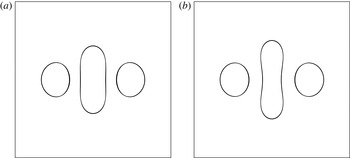
Figure 3 illustrates the shape of two equilibria for an aspect ratio of
 $r/h=3$
for the satellites, with
 $d/h=1$
, and for two values of
 ${\it\delta}/r$
. The case with larger
 ${\it\delta}/r$
(figure 3
a) corresponds to the margin of stability. Tripoles with closer poles are all unstable while tripoles where the satellites are farther away from the core are stable, all other parameters being fixed. The deformation from cylindrical shape is more pronounced for the second case with a smaller gap
 ${\it\delta}/r$
(figure 3
b), as the interaction between the poles is increased. It corresponds to the case with the smallest gap
 ${\it\delta}/r$
obtained in practice. The branch of equilibria may continue beyond this point but may not correspond to a smaller gap
 ${\it\delta}$
which is our control parameter. We are principally interested in this study in the margin of stability, hence we do not attempt to complement the branch by using a new parameter. The shape shown in figure 3 is generic of all cases investigated in our range of parameters. An extension of these results is discussed in appendix C.
Top view of the tripolar equilibria for
 $r/h=3$
,
 $d/h=1$
and
 ${\it\delta}/r={\it\delta}_{m}/r=4.114$
(margin of stability, a),
 ${\it\delta}/r=3.948$
(b).

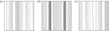
The tripole core, which is nearly cylindrical when the satellites are far apart, tends to be squashed along the tripole axis as the satellites are brought closer together. The core vortex tends towards a dumbbell shape in marginal cases. The deformation of the core boundary is dominated by an azimuthal mode
 $m=2$
, due to the shear created by the satellites. In the rotating frame of reference, the streamline topology coincides with that of the potential vorticity distribution, for steady states.
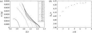
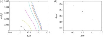
Next, we perform a linear stability analysis on the equilibria. This analysis quantifies wave growth along PV contours (see appendix B). In practice, 10 wavenumbers are used for every contour; details of the approach can be found in the appendix of Reinaud & Dritschel (Reference Reinaud and Dritschel2002) or in Reinaud (Reference Reinaud2015). Figure 4(a) shows the non-dimensional growth rate of the most unstable mode,
 ${\it\sigma}/|q|$
, along the first cross-section of parameters with
 $d/h=1$
and various aspect ratios versus the non-dimensional gap
 ${\it\delta}/r$
. Because we use
 ${\it\delta}/r$
, we actually see the influence of the aspect ratio rather than a mere scaling effect due to the increasing radius (recall that all calculations use explicitly
 $h=1$
, hence in practice
 $r$
and
 $r/h$
are the same). The curves are ordered from left to right, from small aspect ratio corresponding to low values of the marginal gap
 ${\it\delta}_{m}/r$
to larger aspect ratios and larger marginal gaps
 ${\it\delta}_{m}/r$
. This is synthesised in figure 4(b) showing the location of the first unstable mode observed. Thus tripoles with flatter poles are more unstable (as expected for baroclinic instability). This also holds for hetons (see Flierl Reference Flierl1988; Reinaud & Carton Reference Reinaud and Carton2009; Carton et al.
Reference Carton, Flierl, Perrot, Meunier and Sokolovskiy2010a
,Reference Carton, Meunier, Flierl, Perrot and Sokolovskiy
b
). We notice a sharper decrease of the critical gap as the aspect ratio decreases.
Non-dimensional growth rates
 ${\it\sigma}/|q|$
for the first instability mode for
 $d/h=1$
and
 $r/h=2{-}8$
each 0.5 (a). The curves are naturally ordered from left to right as
 $r/h$
increases. The gap
 ${\it\delta}/r$
versus the aspect ratio
 $r/h$
at the margin of stability (b).

Next, we provide the spatial structure of the first most unstable mode. For the range of values of
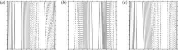
 $r/h$
discussed above, the structure of the mode is the same in all cases and is illustrated in figure 5. The case shown corresponds to
 $r/h=3$
,
 $d/h=1$
and
 ${\it\delta}/r={\it\delta}_{m}/r=4.114$
. The spatial structure of the modal deformation is different for the satellites and the core. It should be recalled that the aspect ratio of the core is
 $\sqrt{2}$
times that of the satellites.
Contours of isodeformation (solid line, positive; dashed line, negative): spatial structure of the first instability mode for
 $r/h=3$
and
 $d/h=1$
at the margin of stability for
 ${\it\delta}/r={\it\delta}_{m}/r=4.114$
. Panels (a–c) correspond to the horizontal location of the vortex (a–c). In each panel, the horizontal axis is the polar angle
 $0<{\it\theta}<2{\rm\pi}$
and the vertical axis is the true vertical.

The core is expected to be sensitive to higher wavenumber instability than in the two-vortex problem, in particular azimuthal mode
 $m=2$
(and its harmonics); the satellites are more deformed on azimuthal mode
 $m=1$
. The growth of azimuthal mode
 $m=2$
(and of its harmonics) deforms the vortex into a dumbbell, which can eventually break up in the nonlinear regime. This also explains the sharp decrease of the critical gap with the aspect ratio observed above for steady states. For hetons, mode
 $m=2$
only appears for wide enough vortices and for small separation between the poles; the critical distance decreases as the aspect ratio of the poles decreases. The same phenomenon repeats here and wider vortices are more sensitive to instability than more compact ones. It should be noted that the predominance of the azimuthal mode
 $m=2$
is also explained by the fact that the deformation of the central pole by the side poles is in fact a deformation consistent with
 $m=2$
; that is, the topology of the flow forces the mode
 $m=2$
. Further tests with
 $r/h$
up to 100 (not shown) confirmed that the central pole eventually breaks following a deformation
 $m=2$
, while other yet weaker modes are present (e.g.
 $m=3$
in combination with
 $m=2$
).
The influence of the vertical offset on the stability of the
 ${\it\Lambda}$
-vortex is examined in figure 6 for
 $r/h=3$
and
 $d/h=0$
, 0.12, 0.24, 0.52, 1, 1.52 and 2. It should be noted that no instability to mode
 $m=2$
has been observed for the larger vertical offsets. As expected, as the vertical offset between the poles increases, the mutual influence of the core and satellites decreases and their tendency to destabilise each other decreases. In other words, the vortices need to be closer horizontally to trigger instability as they are pulled farther apart vertically. Plotting the growth rate as a function of the three-dimensional distance between the satellite and core centres does not change the ordering of the curves, nor do they collapse onto a single one. Indeed, horizontal separations and vertical separations do not play the same role in the shear and strain induced by the poles. This is fundamentally due to the lack of vertical advection in quasi-geostrophy. This adds to the fundamental asymmetry in the shape of the vortices which have small aspect ratio here.
Growth rates for the first instability mode for
 $r/h=3$
, and
 $d/h=0$
, 0.12, 0.24, 0.52, 1, 1.52 and 2 (a). The curves are naturally ordered from left to right as
 $d/h$
decreases. The gap
 ${\it\delta}/h$
is represented versus
 $d/h$
at the margin of stability (b). It should be recalled that
 $h=1$
and
 $r/h=3$
are fixed for all cases in the figure.

It can also be noted that for vertically distant core and satellite, the mutual influence of the lower satellites can determine their stationary shape, which becomes similar to that of two identical vortices in a two-dimensional flow (figure 8, equilibria). Such equilibria were also found by Shteinbuch-Fridman et al. (Reference Shteinbuch-Fridman, Makarov, Carton and Kizner2015) (see also appendix C).
Finally, it should be noted that all configurations with poles located distant enough from one another are stable. This is consistent with the point vortex calculation which indicates that the point vortex problem is linearly stable. Indeed, the strength of the point vortices
 ${\it\kappa}$
divided by the cube of a typical separation distance
 $d_{s}$
between the poles only sets the time scale of the problem (
 $t\sim d_{s}^{3}/{\it\kappa}$
). If the point vortices had unstable configurations, the margin of stability would be determined by the relative distances (ratio of distances) between the poles only. This would mean that all finite-core set-ups where the relative position of the pole centres is the same should be unstable for all pole sizes (or alternatively for a set pole size and all separation distances as long as they are kept within the same relative ratios).
3.3. The nonlinear evolution of cylindrical poles
A tripole comprising three cylindrical poles is used to initialise the nonlinear model. This configuration leads to an unsteady motion: the poles deform. If an equilibrium with similar properties is reachable, the flow should oscillate about it, if the equilibrium is stable (and in the absence of dissipation). Three main evolutions (two of which are of most interest to this study) are observed.
The first evolution has the two satellites inducing shear and strain large enough to break the core into two main vortices, possibly with smaller satellites and debris. These two main poles combine with the lower poles as hetons, which then escape. This interaction was also commonly observed in the head-on collision of hetons, see Reinaud & Carton (Reference Reinaud and Carton2015).
The second main evolution has the
 ${\it\Lambda}$
-tripole exhibiting a quasi-periodic motion, though with strong oscillations (wobbling of the core). The
 ${\it\Lambda}$
-tripole is robust and persists in time. The strain and shear induced by the satellites are not strong enough to break the core.
The third and last evolution occurs when the satellites are close enough to merge. The end state is a baroclinic structure consisting of two vortices which resembles a heton. Such structures have already been investigated and are not the focus of the present study. This evolution corresponds to vortex merger in the strain induced by a third vortex; such problems have been addressed, in particular, by Perrot & Carton (Reference Perrot and Carton2010) and Sokolovskiy, Koshel & Carton (Reference Sokolovskiy, Koshel and Carton2011).
This transition between robust
 ${\it\Lambda}$
-tripoles and a pair of hetons depends on the aspect ratio
 $r/h$
of the poles. Because of the size of the parameter space, we only focus on
 $r/h=3$
and 7. We place the vortices initially at various horizontal and vertical distances
 ${\rm\Delta}x,d$
.
The numerical procedure to simulate the time evolution of the flow is the three-dimensional contour surgery method, see, e.g., Reinaud & Dritschel (Reference Reinaud and Dritschel2009). The fluid domain containing PV is mapped in the vertical by 100 layers. The time integration is performed using a fourth-order Runge–Kutta time stepping with
 $\text{d}t=2{\rm\pi}/(40q)$
following the standard set-up of the method. It should be noted that here
 $q=2{\rm\pi}$
. The time scale of the problem is set by
 $q$
. A sphere of PV
 $q$
has a rotation period of
 $T_{sph}=6{\rm\pi}/|q|$
while an infinite column has a rotation period of
 $T_{col}=4{\rm\pi}/|q|$
.
The time-dependent shape of the vortices is described by the geometrical moments
 $M_{(m,n,p)}$
of order
 $q=m+n+p$
, defined by
 $$\begin{eqnarray}M_{(m,n,p)}=\iiint _{V}(x-x_{c})^{m}(y-y_{c})^{n}(z-z_{c})^{p}\,\text{d}V,\end{eqnarray}$$
with
 $(m,n,p)\in \mathbb{N}^{3}$
. In this definition,
 $x_{c},y_{c}$
and
 $z_{c}$
represent the centre of the vortex analysed. There is only one moment of order zero, the volume of PV of the vortex. The three first-order moments give, after scaling by the volume, the mode-1 deformation of the vortex in all directions. The six independent second-order moments
 $M_{(2,0,0)}$
,
 $M_{(0,2,0)}$
,
 $M_{(0,0,2)}$
,
 $M_{(1,1,0)}$
,
 $M_{(1,0,1)}$
,
 $M_{(0,1,1)}$
give the coefficients of a
 $3\times 3$
symmetric matrix describing the ellipsoid best fitted to the vortex. These moments provide the first information about the shape of the vortex. The eigenvalues of the matrix are the squares of the half-lengths
 $a,b,c$
of the ellipsoid axes, while the associated eigenvectors
 $\boldsymbol{a},\boldsymbol{b},\boldsymbol{c}$
give the directions of the axes. By convention, we order the semiaxis lengths such that
 $a\leqslant b\leqslant c$
. The orientation of the ellipsoid is given by the eigenvectors of the same matrix. Three of the fourth-order moments (namely,
 $M_{(4,0,0)}$
,
 $M_{(0,4,0)}$
and
 $M_{(0,0,4)}$
) are used to illustrate the change in shape of the poles later in the paper.
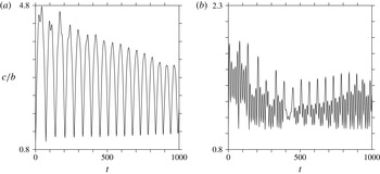
Time evolution of the aspect ratio
 $c/b$
for the best fitted ellipsoids. (a) Core vortex (positive pole 1). (b) One of the satellites (negative pole 2 or 3). The original poles are defined by
 $r/h=3.5$
,
 ${\rm\Delta}x/h=18$
,
 $d/h=0.5$
.

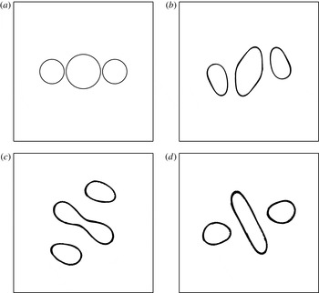
First, we present a nonlinear evolution of the tripoles for which the interaction is not destructive. Then, the vortices may strongly deform, and oscillate with time, but they retain their volume. Figure 7 shows the oscillations of the horizontal aspect ratio
 $c/b$
for the poles when the satellite aspect ratio
 $r/h$
is initially set to 3.5, with
 $d/h=0.5$
and
 ${\rm\Delta}x/h=18$
. The simulation starts from circular contours but the corresponding equilibria have dumbbell-shaped cores. Indeed, the core shape oscillates from nearly circular to elongated (hence
 $c/b>1$
). This is further demonstrated by figure 8, in which the near equilibrium shape is visible. The satellites also slightly oscillate as a result of the pole interaction, yet the amplitude of their oscillations is much less (about half of that of the core vortex). The amplitude of the oscillations decreases with time, possibly indicating convergence towards the equilibrium. However, this process is extremely slow and the oscillations persist for very long times. As a comparison, we have computed an equivalent equilibrium with
 $d/h=0.52$
and
 ${\rm\Delta}x/h\simeq 18$
; the aspect ratio of the equilibria for the core vortex is 2.17, approximately the midvalue of the oscillations of the core vortex aspect ratio at long times. There is no tendency towards axisymmetrisation because the corresponding equilibrium state is not axisymmetric, as shown in the previous section. Then, only strong viscous effects, absent from the current calculation at very high Reynolds number, could induce axisymmetrisation. The case described here corresponds to the smallest horizontal separation
 ${\rm\Delta}x/h$
, with
 $r/h=3.5$
and
 $d/h=0.5$
, for which the tripole persists; it is a marginally non-destructive state.
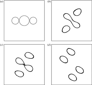
Illustration of a persisting tripole (limit case). Here,
 $r/h=3.5$
,
 ${\rm\Delta}x/h=18$
and
 $d/h=0.5$
, at
 $t=0$
(a), 5 (b), 35 (c) and 115 (d).

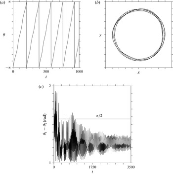
Figure 9 shows the rotation of the whole structure. The satellites exhibit a quasi-periodic rotation pattern around the core vortex, indicating again that the tripole oscillates around an equilibrium state (which would steadily rotate). However, the equilibrium is not exactly reached, as seen from the angular difference between the axis that joins the centres of the satellite vortices
 ${\it\theta}_{2}$
and the orientation axis of the central vortex
 ${\it\theta}_{1}$
. These angles are defined by
 $$\begin{eqnarray}{\it\theta}_{1}={\displaystyle \frac{1}{2}}\arctan \left({\displaystyle \frac{2M_{(1,1,0)}}{M_{(2,0,0)}-M_{(0,2,0)}}}\right)\end{eqnarray}$$
and
 $$\begin{eqnarray}{\it\theta}_{2}=\arctan {\displaystyle \frac{{\rm\Delta}y_{c}}{{\rm\Delta}x_{c}}},\end{eqnarray}$$
where
 ${\rm\Delta}y_{c}$
(respectively
 ${\rm\Delta}x_{c}$
) is the distance between the centres in the
 $y$
-direction (respectively
 $x$
-direction) of the lower poles. The centres of the poles are themselves determined by volume integration,
 $(x_{c},y_{c})=(\iiint _{V}x\,\text{d}V,\iiint _{V}y\,\text{d}V)/\iiint _{V}\,\text{d}V$
. If the tripole had reached an exact equilibrium, the angular difference should settle to
 ${\rm\pi}/2$
, as seen from the shape of the equilibria determined in the previous section. However, there is a residual unsteadiness remaining due to the fact that the vortices have not been able to adapt their shape completely. This may be related to a lack of filamentation of the core vortex in the final stage; thus, this pole is too elongated and rotates too slowly compared with the whole tripolar structure. This, in turn, generates the mode
 $m=3$
and
 $m=4$
deformations seen on the core and satellite contours.
Tripole. (a) Time evolution of the angle
 ${\it\theta}_{2}$
of the axis joining the satellite centres. (b) Quasi-periodic trajectory of satellite 2. The original tripole is defined by
 $r/h=3.5$
,
 ${\rm\Delta}x/h=18$
,
 $d/h=0.5$
. The pseudoperiods for one rotation are
 $T=203$
(first),
 $T=189$
(second),
 $T=182$
(third),
 $T=180$
(fourth) and
 $T=174.5$
(fifth). (c) Time evolution of the angular difference between the orientation angle
 ${\it\theta}_{1}$
of the main horizontal axis of the ellipsoidal shape of the central vortex and
 ${\it\theta}_{2}$
.

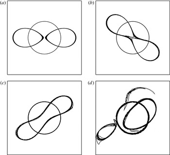
Next, we illustrate in figure 10 the nonlinear evolution of the tripole for the same geometry, i.e.
 $r/h=3.5$
and
 $d/h=0.5$
, but with a slightly smaller horizontal separation
 ${\rm\Delta}x/h=17.75$
. In this case the strain induced by the satellites on the core is stronger and is large enough to break it. For equivalent equilibria, this corresponds to an unstable azimuthal mode
 $m=2$
on the core vortex. Indeed, the core vortex is initially deformed by the satellites into a dumbbell shape, as in the previous case, but this deformation keeps on increasing until the core vortex breaks into two parts. These parts then pair with the poles at the bottom, and form hetons which escape. This nonlinear evolution of the tripole is consistent with the linear stability analysis of the equilibria. The core vortex breaking is consistent with the development of a mode
 $m=2$
while the satellites are less deformed (contrarily to the equilibria, they are affected by the time-dependent oscillations of the aspect ratio of the core vortex).
Illustration of a breaking tripole (limit case). Here,
 $r/h=3.5$
,
 ${\rm\Delta}x/h=17.75$
and
 $d/h=0.5$
, at
 $t=0$
(a), 30 (b), 35 (c) and 70 (d).

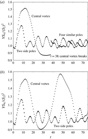
The time evolution of the last two examples is further illustrated in figure 11, where the non-dimensional kurtosis of the moments,
 $$\begin{eqnarray}\displaystyle {\displaystyle \frac{VS_{4}}{(S_{2})^{2}}}=V{\displaystyle \frac{M_{(4,0,0)}+M_{(0,4,0)}+M_{(0,0,4)}}{(M_{(2,0,0)}+M_{(0,2,0)}+M_{(0,0,2)})^{2}}}, & & \displaystyle\end{eqnarray}$$
versus time is presented for each of the large structures identified. Here,
 $V$
denotes the volume of each structure. Debris with volume much smaller than the main vortices is not displayed for clarity. All major steps of the interactions can be identified. This figure shows that the core deformation (on mode
 $m=4$
) is only slightly larger for hetonic breaking than for tripolar evolution. It should be noted that
 $m=4$
is the harmonic of
 $m=2$
and is thus generated by nonlinear interactions of the latter. Thus, there is a threshold in the possible elongation and deformation of the core allowed for tripoles to survive. Again, this is related to the fact that, in a steady tripole, the elliptical core must rotate at the same rate as the whole structure, and thus cannot be too elongated. Furthermore, too elongated a core will break.
Tripoles: time evolution of
 $VS_{4}/S_{2}^{2}$
in the case
 $r/h=3.5$
,
 $d/h=0.5$
and
 ${\rm\Delta}x/h=17.75$
(a) and
 ${\rm\Delta}x/h=18$
(b).

It should be noted also that the evolution of all pole deformations is nearly the same for breaking and non-breaking cases, until core breaking has occurred.
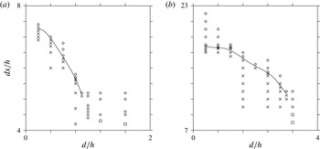
Figure 12 summarises the different regimes observed from the nonlinear simulations, starting with cylindrical poles for the two cases
 $r/h=3.5$
and 7. Results are plotted in the parameter space
 $d/h$
,
 ${\rm\Delta}x/h$
. They confirm the results from the linear stability analysis of the equilibria. The central vortex can break into two smaller poles as a consequence of a mode
 $m=2$
instability. For this instability to be triggered, the distance between the poles needs to be smaller than a certain threshold. For small vertical gaps
 $d/h$
, there exist (at least) two different regimes. For small values of
 ${\rm\Delta}x/h$
, the core vortex can destabilise due to the strain induced by the satellite vortices; the core then breaks into two smaller vortices. For larger values of
 ${\rm\Delta}x/h$
, the core vortex is stable, as it is for larger vertical gaps
 $d/h$
. This is in agreement with the results of the linear stability analysis. When the core vortex is stable, two new regimes are observed. In the first one, the two satellites can merge. The tripole then transforms into a heton. A similar behaviour can be observed for even smaller gaps, in competition with the breaking of the upper pole. For larger values of
 ${\rm\Delta}x/h$
, the vortices no longer merge, nor is the central vortex destabilised, and the tripole remains an oscillating tripole. This is expected to be generic for all such tripolar structures. When the poles are well separated in either the vertical or the horizontal direction, the tripolar structure is expected to be stable, while the central vortex is expected to break into (at least) two parts for smaller separation distances.
Tripoles: regime diagram for
 $r/h=1.5$
(a) and
 $r/h=3.5$
(b). The diamonds indicate a persisting tripole, the crosses indicate a breaking tripole and the squares indicate the merging of the two negative lower poles.

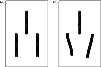
Finally, another mode of instability is observed for tall poles; it is related to a horizontal azimuthal mode
 $m=1$
. Such a mode corresponds to the tilting or bending of the vortices. This mode can be found in the linear stability analysis of tall equilibria; however, we do not investigate it in detail. To accurately represent tall vortices and to capture this weak mode, a very large number of layers is necessary. This leads to a very high calculation cost, too expensive for a detailed parametric study. An example of this mode is given in figure 13 for
 $r/h=0.5$
and
 $d/h=0$
. It should be noted that such a mode is not observed for
 $r/h\geqslant 2$
. In the example provided, the tilting is, in practice, so small that the nonlinear evolution of the case does not show any major deformation or wobbling of the vortices.
Contour of isodeformation (solid line, positive; dashed-line, negative): spatial structure of the tilting instability mode for
 $r/h=0.5$
,
 $d/h=0$
and
 ${\it\delta}/h=2.207$
(this gap is defined from the lowermost contours). Here, each pole is sampled by 150 layers.

This mode can also be illustrated using a nonlinear simulation starting with tall cylinders (see figure 14 for a case with
 $r/h=0.1$
,
 $d/h=0$
,
 ${\rm\Delta}x/h=0.8$
). The top of the satellites wobbles widely, but, by symmetry, the core vortex does not. The strong deformation is not destructive in this case. For smaller
 ${\rm\Delta}x$
, the deformation leads parts of the satellites close to each other, and these parts merge. The columnar satellites break vertically into pieces, with a central part merging and aligning with the core vortex.
Tall tripoles:
 $r/h=0.1$
,
 $d/h=0$
and
 ${\rm\Delta}x/h=0.8$
, at
 $t=0$
(a) and 35 (b). The vortices are viewed stereographically at an angle of
 $60^{\circ }$
from the vertical.

4. Formation of tripolar structures from heton collisions
In the previous sections, the robustness of tripolar vortices was analysed using both linear stability analysis of equilibrium states and nonlinear simulations of generic cylindrical tripoles. Tripoles can either be robust for long times, or the central vortex may be unstable to a horizontal azimuthal mode
 $m=2$
and break under the strain induced by the satellites.
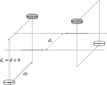
Here, we examine one possible mechanism for the formation of such tripoles. Other mechanisms of formation may be possible, such as the asymmetric destabilisation of hetons with unequal poles, but this is beyond the scope of the present paper. The mechanism considered in the present paper consists in the collision of two hetons with offset translation axes. The configuration is illustrated in figure 15. The two identical hetons consist initially of two cylindrical poles of the same volume and the same PV magnitude, with an aspect ratio
 $r/h$
. They move in opposite directions. Here, we focus on the formation of tripolar structures, hence we place the like-signed poles at the same height. This is referred to as the symmetric configuration. The antisymmetric configuration where opposite-signed poles are at the same depth would not generate tripolar structures and will be the focus of another study. Within each heton, the poles are separated vertically by
 $d$
, as in the previous sections, and horizontally by
 $d_{y}$
. The hetons as a whole are offset by a distance
 $d_{s}$
in the horizontal. Thus, the upper poles are initially separated in the
 $y$
-direction by
 $d_{y}-d_{s}$
while the lower poles are separated by
 $d_{y}+d_{s}$
.
Geometry of the offset hetons in a symmetric configuration. The vertical centroid separation between the lower and upper poles, denoted
 $d_{z}$
, is linked to the pole separation
 $d$
, with
 $d_{z}=d+h$
.

Because of the large parameter space, only situations likely to form a
 ${\it\Lambda}$
-vortex are studied here. This imposes the following a priori conditions. First, the hetons should not be prone to baroclinic instability. Thus, the poles of each heton should be spaced sufficiently, vertically (by
 $d$
) and horizontally (by
 $d_{y}$
). Indeed, unstable hetons may break into smaller vortices before they can interact. By offsetting the two hetons horizontally (by
 $d_{s}\sim d_{y}$
), the two upper poles almost face each other initially and have more chance to merge as they collide. Keeping
 $d_{y}$
large enough prevents the two lower poles from merging during the interaction.
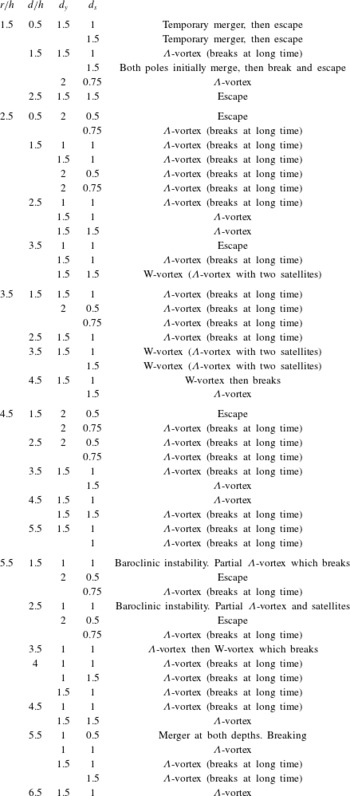
A full list of simulations performed, with a short description of the outcome, is given in appendix D. The formation of a
 ${\it\Lambda}$
-vortex is a very common occurrence in the relevant part of the parameter space described above. We propose here a more detailed description of four different regimes observed.
In the first example,
 $r/h=1.5$
 $d/h=2.5$
with
 $d_{y}/r=1.5$
and
 $d_{s}/d_{y}=1.5$
. In this case the hetons are compact with
 $r/h$
moderate and the poles within the hetons are well separated (large
 $d$
). Each heton is originally stable and the poles do not significantly deform with time. Because the hetons are well separated in the horizontal, they do not get close enough for the upper poles to merge. Instead, during close encounter, the upper poles rotate and modify their relative position within each heton. This changes the direction of propagation, and the hetons escape at an angle from their initial direction. This is illustrated in figure 16. This evolution is generic to all cases where the hetons are initially stable and are well separated horizontally.
Weak interaction between two offset hetons with
 $r/h=1.5$
,
 $d/h=2.5$
,
 $d_{y}/r=1.5$
and
 $d_{s}/d_{y}=1.5$
, at
 $t=25$
(a) and 140 (b). The vortices are viewed from the top.

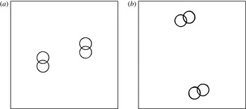
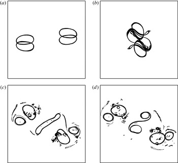
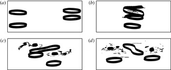
The following example, shown in figure 17, illustrates the formation of an unstable tripole. In this case, the original hetons have
 $r/h=1.5$
with
 $d/h=1.5$
,
 $d_{y}/r=1.5$
,
 $d_{s}/d_{y}=1.5$
. The only difference from the former situation is that the poles are initially closer vertically. This has two consequences.
Formation of a temporary tripole from hetons with
 $r/h=1.5$
,
 $d/h=1.5$
,
 $d_{y}/r=1.5$
and
 $d_{s}/d_{y}=1.5$
, at
 $t=25$
(a), 60 (b), 80 (c) and 140 (d). The vortices are viewed from the top.

First, the poles may deform more before the interaction because each heton is more sensitive to baroclinic modes. However, the main effect is to make the heton move faster. Thus, the upper poles get closer before their trajectory is altered by mutual interaction, and, in fact, close enough to merge. However, because
 $d_{y}/d_{s}=1.5$
, the upper poles face each other (this is also due to an originally curved trajectory). Using a numerical tool identifying all regions of PV anomaly and calculating their properties, we note that, before interaction, the unstable contour modes initially lead to the shedding of a negligible amount of fluid. Then, at
 $t=67.5$
the two upper poles merge to form a single structure of twice the volume of the original vortices. This interaction forms a large amount of small debris and filaments, which keep being generated as the final structure is not stable. Eventually, by
 $t=131$
the upper large vortex breaks asymmetrically; this produces even more debris and filaments. The largest part of the two new upper vortices has a volume approximately 50 % larger than the volume of each satellite. These satellites have shed little PV during the interaction. The volume of the second part of the central vortex is approximately half the volume of the satellites. Further interactions finally create six main PV structures and a great deal of debris and small-scale structures.
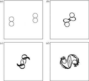
To create a more robust tripole,
 $d_{y}$
is increased to stabilise the hetons individually, and
 $d_{s}/d_{y}$
is decreased to make the upper poles collide head on, favouring the formation of a more robust structure. The parameters are
 $r/h=1.5$
,
 $d/h=1.5$
, as in the previous case, but
 $d_{y}/r=2$
and
 $d_{s}/d_{y}=0.75$
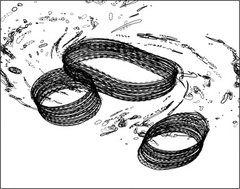
. The evolution, displayed in figure 18, shows that indeed the upper poles almost face each other during collision, and generate a strong core which remains metastable for a long time. A three-dimensional view of the tripole is displayed in figure 19. At
 $t=40$
, the upper poles have merged into a structure twice the size of the original vortices, and by the end of the simulation, at
 $t=400$
, the upper core still contains 90 % of its original volume, having only shed 10 % through filamentation.
Formation of a robust tripole from hetons with
 $r/h=1.5$
,
 $d_{z}/h=1.5$
,
 $d_{y}/r=2$
and
 $d_{s}/d_{y}=0.75$
, at
 $t=0$
(a), 40 (b), 45 (c) and 80 (d). The vortices are viewed from the top.

Robust tripole resulting from hetons with
 $r/h=1.5$
,
 $d/h=1.5$
,
 $d_{y}/r=2$
and
 $d_{s}/d_{y}=0.75$
. The tripole is viewed at an angle of
 $60^{\circ }$
from the vertical.

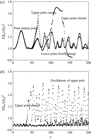
In figure 20, we next plot the ratio
 $VS_{4}/(S_{2})^{2}$
to illustrate the differences between the formation of a robust tripolar structure and the formation of an unstable tripolar structure. The unstable structure forms a great deal of debris and has stronger deformations, while the stable structure has a more regular and less deformed evolution.
Tripoles: time evolution of
 $VS_{4}/(S_{2})^{2}$
in the case of an unstable tripole formation (a) with
 $r/h=1.5$
,
 $d/h=1.5$
,
 $d_{y}/r=1.5$
and
 $d_{s}/d_{y}=1.5$
, and for a robust tripole (b) with
 $r/h=1.5$
,
 $d/h=1.5$
,
 $d_{y}/r=2$
and
 $d_{s}/d_{y}=0.75$
.

Finally, for flatter hetons (larger aspect ratios
 $r/h$
), the upper core of the resulting tripole may destabilise differently. Instead of breaking into two parts, it sheds two lateral vortices from the tip of its most elongated axis. These satellites align with the lower satellites. The final structure is composed of five main vortices, rather than three for the tripole; these poles are distributed as a W; it is metastable and persists for a longer time. An example is provided in figure 21, where
 $r/h=7$
,
 $d/h=7$
,
 $d_{y}/r=1.5$
and
 $d_{s}/d_{y}=1.5$
. It should be noted that the vertical offset is large to stabilise the original hetons, as the poles are very flat, and hence very sensitive to baroclinic modes.
Robust W-vortex resulting from hetons with
 $r/h=3.5$
,
 $d/h=3.5$
,
 $d_{y}/r=1.75$
and
 $d_{s}/d_{y}=1.5$
, at
 $t=25$
(a), 75 (b), 100 (c) and 160 (d). The structure is viewed orthographically at an angle of
 $75^{\circ }$
from the vertical.

In this evolution, the upper poles merge at
 $t=65.5$
. Then, only three vorticity poles are present, the upper core and the two lower satellites. However, the tripole is unstable, and starting from
 $t=76.6$
, the upper core sheds some PV. At
 $t=82$
four main structures are clearly identifiable with volumes
 $V_{1}(t=82)/V_{v}(t=0)\sim 1.68$
for the main part of the upper core, and
 $V_{2}(t=82)/V_{v}(t=0)\sim V_{3}(t=82)/V_{t}(t=0)\sim 1$
for the lower satellites, where
 $V_{v}(t=0)$
is the volume of the original poles. The two other upper vortex structures have similar volumes
 $V_{4}/(t=82)V_{v}(t=0)\sim V_{5}(t=82)/V_{v}(t=0)\sim 15\,\%$
. The remaining PV is distributed in very small debris and filaments. It should be noted that at
 $t=82$
the centroid of the lower satellites is located at
 $(0.15,-1.43,-0.41)$
(respectively
 $(-0.16,1.44,0.41)$
), and the two upper satellites lie at
 $(0.26,-1.44,0.41)$
(respectively
 $(-0.26,1.45,0.41)$
). This shape justifies the W-vortex name for this multipole.
5. Conclusion
We have studied the equilibria and linear stability of baroclinic tripoles, which can result from the collision of horizontally offset hetons. Baroclinic tripolar equilibria can exist and persist for a long time as stable structures, provided that the aspect ratio of the poles is approximately unity. For flatter poles, baroclinic instability modes may grow and the vortices may break. Indeed, the linear stability analysis of equivalent point tripoles shows that infinitesimal perturbations are not sufficient to break the tripoles. Instability originates from the finite size of the poles, and from their finite-amplitude deformation. The upshot is that tripoles whose poles are well separated in either the horizontal direction or the vertical direction are stable. This is due to the fact that the strain induced by the (smaller) side vortices is not strong enough to break the central (larger) vortex. The stability also relies on the ability of the central vortex itself to be destabilised. The mode of instability that breaks the central vortex has an azimuthal wavenumber
 $m=2$
. This mode is in fact forced by the topology of the flow (induced by the two side vortices). However, for compact vortices (
 $r/h$
small), no instability to mode
 $m=2$
is found. This is not dissimilar to the known fact that hetons with small aspect ratios are stable, see Reinaud & Carton (Reference Reinaud and Carton2009). Finally, tall poles may be unstable to tilting instability. Such instabilities can be related to similar modes observed in tall columns in shear (Dritschel & de la Torre Juárez Reference Dritschel and de la Torre Juárez1996) and for two interacting tall vortices (see Reinaud & Dritschel Reference Reinaud and Dritschel2005).
The formation of baroclinic tripoles from the collision of two hetons can be seen as a mechanism (temporarily) halting the transport of tracers in the flow. However, due to instabilities, the tripoles may break back into two separate hetons. Such hetons would resume their translation and thus transport the tracers across the domain. The direction in which the new dipoles move depends, in particular, on the relative position of the poles as they are formed.
Moderately offset hetons, translating in opposite directions and colliding, efficiently form baroclinic tripoles. Nevertheless, other evolutions are possible: heton collision can lead to new hetons if the upper poles do not merge; it can also lead to the vertical breaking of the poles if they are tall; finally, the upper core of the tripole can shed smaller vortices which co-rotate with the original tripole to form a W-vortex. This last evolution is interesting as an example of the formation and long survival of the so-called ‘submesoscale’ vortices, as they are stabilised by other PV structures.
From the moderate range of parameters spanned in this study (see also table 1 in appendix D), we conclude that hetons whose poles are well offset initially are likely to escape without forming a tripolar structure. When the poles of the hetons are moderately offset so that the horizontal offset between the poles is of the same order as the horizontal separation distance between the poles (such that two of the same-depth poles are facing each other), a tripolar structure is likely to form. This formation is only temporary if the merger of the two poles is only partial and/or if the resulting pole is large enough to be sensitive to the instability with azimuthal mode
 $m=2$
observed in tripolar structures. Finally, very wide incoming hetons may be sensitive to baroclinic modes of instability prior to the interaction and yield to more complex behaviour.
Other tripole formation mechanisms could be investigated further, in particular the instability of a vertically asymmetric perturbed and baroclinically unstable vortex. This will be addressed in the future.
This paper has not detailed the conditions of vortex merger under external strain. Although this problem has received attention in two dimensions and in two layers, the general three-dimensional problem has not been investigated yet to the best of our knowledge.
Moreover, other heton collision configurations are possible, in which the same-depth poles have opposite polarities. Vortex merger is then prohibited, but the like-signed vortices at different depths may align vertically (this may lead to a Z-shaped tripole already observed in two-layer flows). This is the subject of a study to follow.
Appendix A. Point vortex stability
We start with the velocity field induced by the displaced source vortex
 $({\it\kappa}_{s},x_{s}+x_{s}^{\prime },y_{s}+y_{s}^{\prime },z_{s})$
on the displaced target vortex
 $({\it\kappa}_{t},x_{t}+x_{t}^{\prime },y_{t}+y_{t}^{\prime },z_{t})$
in the fixed frame. It should be noted that we only take into account horizontal perturbations. These are the only ones consistent with quasi-geostrophic dynamics (there is no vertical advection in quasi-geostrophy).
 $$\begin{eqnarray}\displaystyle \boldsymbol{u}(\boldsymbol{x}) & = & \displaystyle (-(y_{t}-y_{s})-(y_{t}^{\prime }-y_{s}^{\prime }),(x_{t}-x_{s})+(x_{t}^{\prime }+x_{s}^{\prime }))\nonumber\\ \displaystyle & & \displaystyle \times \,\frac{{\it\kappa}_{s}}{((x_{t}-x_{s})+(x_{t}^{\prime }-x_{s}^{\prime }))^{2}+((y_{t}-y_{s})+(y_{t}^{\prime }-y_{s}^{\prime }))^{2}+((z_{t}-z_{s})^{2})^{3/2}}.\end{eqnarray}$$
Denoting
 $$\begin{eqnarray}r=\sqrt{(x_{t}-x_{s})^{2}+(y_{t}-y_{s})^{2}}\end{eqnarray}$$
and
 $$\begin{eqnarray}\displaystyle & \displaystyle {\it\alpha}=(z_{t}-z_{s})/r, & \displaystyle\end{eqnarray}$$
 $$\begin{eqnarray}\displaystyle & \displaystyle ((x_{t}-x_{s})^{2}+(y_{t}-y_{s})^{2}+(z_{t}-z_{s})^{2})^{3/2}=r^{3}(1+{\it\alpha}^{2})^{3/2}, & \displaystyle\end{eqnarray}$$
 $$\begin{eqnarray}\displaystyle u & = & \displaystyle {\displaystyle \frac{-{\it\kappa}}{r^{3}(1+{\it\alpha}^{2})^{3/2}}}\left((y_{t}-y_{s})+(y_{t}^{\prime }-y_{s}^{\prime })-3{\displaystyle \frac{(x_{t}-x_{s})(y_{t}-y_{s})}{r^{2}(1+{\it\alpha}^{2})}}(x_{t}^{\prime }-y_{s}^{\prime })\right.\nonumber\\ \displaystyle & & \displaystyle \left.-\,3{\displaystyle \frac{(y_{t}-y_{s})^{2}}{r^{2}(1+{\it\alpha}^{2})}}(y_{t}^{\prime }-y_{s}^{\prime })+\cdots \,\right),\end{eqnarray}$$
 $$\begin{eqnarray}\displaystyle v & = & \displaystyle {\displaystyle \frac{{\it\kappa}}{r^{3}(1+{\it\alpha}^{2})^{3/2}}}\left((x_{t}-x_{s})+(x_{t}^{\prime }-x_{s}^{\prime })-3{\displaystyle \frac{(x_{t}-x_{s})^{2}}{r^{2}(1+{\it\alpha}^{2})}}(x_{t}^{\prime }-x_{s}^{\prime })\right.\nonumber\\ \displaystyle & & \displaystyle \left.-\,3{\displaystyle \frac{(x_{t}-x_{s})(y_{t}-y_{s})}{r^{2}(1+{\it\alpha}^{2})}}(y_{t}^{\prime }-y_{s}^{\prime })+\cdots \,\right).\end{eqnarray}$$
For the system of three interacting point vortices of strength
 $\times$
location (
 $-{\it\kappa}$
,
 $-x_{0}$
, 0, 0) for vortex 1,
 $(2{\it\kappa},0,0,z_{0})$
for vortex 2 and
 $(-{\it\kappa},x_{0},0,0)$
for vortex 3, and denoting
 $a=(1+(z_{0}/x_{0})^{2})^{-1/2}$
and
 $b={\it\kappa}/x_{0}^{3}$
, we obtain for the perturbations
 $(x_{i}^{\prime },y_{i}^{\prime })=(\tilde{x_{i}^{\prime }},\tilde{y_{i}^{\prime }})\text{e}^{b{\it\sigma}t}$
,
 $i=-1,2,3$
,
 $$\begin{eqnarray}\displaystyle & & \displaystyle \left(\begin{array}{@{}cccccc@{}}0 & 0 & 0 & -1/8 & 2a^{3} & -1/8\\ 0 & 0 & 0 & -a^{3} & 4a^{3}-1/4 & -a^{3}\\ 0 & 0 & 0 & -1/8 & 2a^{3} & -1/8\\ 1/2-6a^{5} & 6a^{5}-2a^{3} & -1/4 & 0 & 0 & 0\\ -3a^{5}+a^{3} & 6a^{5}-4a^{3}+1/4 & -3a^{5}+a^{3} & 0 & 0 & 0\\ -1/4 & 6a^{5}-2a^{3} & 1/2-6a^{5} & 0 & 0 & 0\end{array}\right)\left(\begin{array}{@{}c@{}}\tilde{x_{1}^{\prime }}\\ \tilde{x_{2}^{\prime }}\\ \tilde{x_{3}^{\prime }}\\ \tilde{y_{1}^{\prime }}\\ \tilde{y_{2}^{\prime }}\\ \tilde{y_{3}^{\prime }}\end{array}\right)\nonumber\\ \displaystyle & & \displaystyle \quad ={\it\sigma}\left(\begin{array}{@{}c@{}}\tilde{x_{1}^{\prime }}\\ \tilde{x_{2}^{\prime }}\\ \tilde{x_{3}^{\prime }}\\ \tilde{y_{1}^{\prime }}\\ \tilde{y_{2}^{\prime }}\\ \tilde{y_{3}^{\prime }}\end{array}\right).\end{eqnarray}$$
The eigenvalues
 ${\it\sigma}_{k}$
satisfy
 $$\begin{eqnarray}{\it\sigma}_{k}^{2}[(4{\it\sigma}_{k})^{2}+((2a-1)(4a^{2}+2a+1))^{2}]^{2}=0,\end{eqnarray}$$
and hence are
 $$\begin{eqnarray}{\it\sigma}_{k}=0,\quad \pm \text{i}(2a-1)(4a^{2}+2a+1)/4=\pm \text{i}((2a)^{3}-1)/4.\end{eqnarray}$$
Appendix B. Notes on obtaining equilibria and their linear stability
We present some technical details related to the calculation of equilibrium states as well as their linear stability. In order to obtain equilibrium states numerically, we use a numerical technique, originated in two dimensions by Pierrehumbert (Reference Pierrehumbert1980), further developed by Dritschel (Reference Dritschel1985) and adapted to three-dimensional flows for two rotating (Reinaud & Dritschel Reference Reinaud and Dritschel2002) or translating (Reinaud Reference Reinaud2015) vortices, adapted here to the three-vortex problem. The method makes the PV jumps that bound the uniform PV vortices converge to streamlines in a frame rotating with the vortices. Both the shape and the rotation rate are obtained from calculation for fixed volumes and location of the structures. In practice, the location of the structures corresponds to a set distance between the outermost edge of the side vortex on the left and the outermost right edge of the central vortex and is denoted
 ${\it\delta}$
, see figure 2. When the contours have converged to streamlines in the relevant rotating frame, as the horizontal velocity field is tangent to the vortex boundaries, the poles do not deform, hence the vortices are in mutual equilibrium. In practice, we first set the aspect ratios of the vortices and the vertical offset between the two side lower vortices and the upper central one. Starting with the side vortices far apart, we initiate the calculation with cylindrical vortices. It should be noted that if infinitely distant, cylindrical poles should be in equilibrium. Indeed, any isolated radial distribution of PV is an equilibrium state. The initial guess is corrected by the algorithm until it reaches an equilibrium, as stated above. Once one equilibrium is obtained, the side vortices are pushed slightly together and the algorithm is resumed to find a new equilibrium for the new separation distance. We therefore obtain a full family of equilibria spanned by a horizontal distance for prescribed aspect ratios and vertical offsets. Several families corresponding to various aspect ratios and vertical offsets are sought. However, to achieve high accuracy in the equilibrium shape, many iterations are needed in the iterative process (typically of the order of 100 such that the correction of the rotating rate in the iterative method becomes less that
 $10^{-12}$
). Each iteration computes the velocity field and streamfunction induced by the vortices in a Lagrangian way by contour integration along the vortex boundaries. If
 $n_{p}$
nodes map the three vortices, the calculation cost grows with
 $n_{p}^{2}$
. As a consequence, finding actual equilibria is expensive numerically and we restrain our attention to a limited number of families, but investigate both the influence of the aspect ratio
 $r/h$
of the poles as well as the influence of the vertical offset
 $d/h$
between the poles. Each vortex is mapped by
 $n_{c}=25$
contours. Each contour is itself mapped by
 $n$
points, and the value of
 $n$
is deduced from the aspect ratio and the
 $n_{c}$
to conserve an accurate horizontal discretisation.
We restrain our attention in this study to symmetric situations. For that purpose we impose first a symmetry of all contours with respect to the
 $x$
-axis along which the centres of the vortices align. Second, the side vortex on the right is taken to be the mirror image of the vortex to the left with respect to the
 $y$
-axis. This also implies that the central vortex is symmetric with respect to the
 $y$
-axis and also that this symmetry is not explicitly imposed but is a consequence of the symmetry of the side vortices. We believe that other equilibria with different symmetries or even asymmetric equilibria may exist, but they are not the focus of the present study.
The stability analysis of the equilibria is based on the analysis of small deformations to the contours bounding the poles, and stems from the two-dimensional version by Polvani & Dritschel (Reference Polvani and Dritschel1993). The perturbed boundary of a contour
 $\mathscr{C}_{k}$
is defined by
 $$\begin{eqnarray}{\bf\rho}_{k}({\it\phi}_{k},t)={\bf\rho}_{e,k}({\it\phi}_{k})+{\it\gamma}_{k}({\it\phi}_{k},t)\frac{\{\text{d}y_{e,k}/\text{d}{\it\phi}_{k},-\text{d}x_{e,k}/\text{d}{\it\phi}_{k}\}}{(\text{d}x_{e,k}/\text{d}{\it\phi}_{k})^{2}+(\text{d}y_{e,k}/\text{d}{\it\phi}_{k})^{2}},\end{eqnarray}$$
where
 ${\it\phi}_{k}$
is the ‘travel time coordinate’, i.e. a quantity proportional to the time that a fluid particle takes to travel along the contour
 $\mathscr{C}_{k}$
;
 ${\bf\rho}_{e,k}\equiv (x_{e,k},y_{e,k})$
is the horizontal position vector describing the equilibrium and
 ${\it\gamma}_{k}$
is the perturbation in the normal direction to the contour
 $\mathscr{C}_{k}$
. The perturbation equation is
 $$\begin{eqnarray}\frac{\partial {\it\gamma}_{k}}{\partial t}+{\it\Omega}_{e,k}\frac{\partial {\it\gamma}_{k}}{\partial {\it\phi}_{k}}=-\mathop{\sum }_{l=1}^{n_{c}}q_{l}\frac{\partial }{\partial {\it\phi}_{k}}\oint _{\mathscr{C}_{l}}{\it\gamma}_{l}G_{k,l}({\it\varrho})\,\text{d}{\it\phi}_{l}^{\prime },\end{eqnarray}$$
where
 $G_{k,l}({\it\varrho})$
is the Green’s function giving the velocity induced in the layer containing the contour
 $\mathscr{C}_{k}$
by the PV within the contour
 $\mathscr{C}_{l}$
,
 $q_{l}$
is the PV jump across
 $\mathscr{C}_{l}$
,
 ${\it\Omega}_{e,k}$
is the constant rotation rate of fluid particles along
 $\mathscr{C}_{k}$
and
 ${\it\varrho}=|{\bf\rho}_{e,k}({\it\phi}_{k})-{\bf\rho}_{e,l}({\it\phi}_{l}^{\prime })|$
denotes the horizontal distance between the contour points.
The perturbation function
 ${\it\gamma}_{k}$
is expanded in a truncated Fourier series expansion
 $$\begin{eqnarray}{\it\gamma}_{k}({\it\phi}_{k},t)=\text{e}^{{\it\sigma}t}\mathop{\sum }_{m=1}^{M}A_{k,m}\cos (m{\it\phi}_{k})+B_{k,m}\sin (m{\it\phi}_{k}).\end{eqnarray}$$
Here, we use
 $M=10$
azimuthal modes.
Appendix C. Other equilibria
Shteinbuch-Fridman et al. (Reference Shteinbuch-Fridman, Makarov, Carton and Kizner2015) obtained a few equilibria with a different shape: the two satellites organised as a figure of 8. In fact, these authors focused on a different part of the parameter space. For these equilibria, the most deformed poles are the lower satellites, which exhibit the same inner sharp edge as for two identical co-rotating vortices. Such equilibria have been extensively studied in Reinaud & Dritschel (Reference Reinaud and Dritschel2002, Reference Reinaud and Dritschel2005), Bambrey, Reinaud & Dritschel (Reference Bambrey, Reinaud and Dritschel2007) and Ozugurlu, Reinaud & Dritschel (Reference Ozugurlu, Reinaud and Dritschel2008).
Here, for tripolar structures, such elongated satellites are recovered when the influence of the upper core is decreased. Keeping the same geometry for the poles, this is achieved by increasing the vertical distance between the poles. An example is provided in figure 22, which belongs to a branch of equilibria for
 $r/h=1$
,
 $d/h=6$
. The topology of the streamlines (initially visible from the shape of the vortex boundaries) is dominated by the interaction of the lower satellites. We ran a nonlinear simulation starting from this unstable steady state. The two satellites temporarily merge before breaking up asymmetrically. The initial evolution of the flow is somehow similar to that of an isolated pair of co-rotating vortices. However, the upper core has an influence over the merger process. The study of this influence may be the topic of a following study, but is not detailed in the present contribution.
Nonlinear evolution of a strongly unstable tripolar equilibrium with
 $r/h=1$
and
 $d/h=6$
, at
 $t=0$
(a), 5 (b), 15 (c) and 55 (d). The vortices are viewed from the top.

Appendix D. List of heton interaction simulations and table of their outcomes
In this appendix, table 1 summarises the outcomes of the main numerical experiments among those achieved during this research.
Table summarising the behaviour of a pair of interacting symmetric hetons;
 ${\it\rho}$
is the aspect ratio of the vortices.