1 Introduction
Multivariate analysis is now a cornerstone in probability theory. Constructing multivariate distributions from given marginals is mathematically interesting on its own, but also has a huge impact in practical problems.
Let
 $d\geq 1$
be an integer, and let
 $X_1, \dots, X_d$
be continuous random variables with cumulative distribution functions (CDFs)
 $F_1,
\dots, F_d$
, respectively. Sklar’s theorem Reference Sklar[36] states that the joint distribution H of
 $(X_1, \dots, X_d)$
can be written, for all
 $$({x_1}, \ldots ,{x_d}) \in {{\mathbb {R}}^d},$$
in the form
 \begin{align*}
H(x_1, \dots, x_d) = {\mathbb{P}}[{X_1\leq x_1, \dots, X_d\leq x_d}] = C(F_1(x_1),
\dots, F_d(x_d)),
\end{align*}
where C is a copula function, i.e. the cumulative distribution function of a probability measure on
 ${\mathbb{R}}^d$
whose marginals are uniform on [0,1]. Copula models are of particular interest because, as seen from the previous equation, they separate the study of the margins and the study of the dependence structure.
In this paper we want to investigate the link between the joint law of a d-dimensional random vector and the law of its multivariate marginals. For any subset
 $K=(j_1,\dots, j_k)$
of
 $\{1,\dots,d\}$
with cardinal k, and any random vector
 $X=(X_1, \dots, X_d)$
, we will write
 $X_K$
to denote the random vector with values in
 ${\mathbb{R}}^k$
given by
 $(X_{j_1}, \dots, X_{j_k})$
and
 $F_K$
the cumulative distribution function of
 $X_K$
. We will abuse notation and call
 $F_K$
a probability distribution on
 ${\mathbb{R}}^k$
. Let
 $n\leq 2^d$
be a positive integer, and let
 $K_1, \ldots, K_n$
be n subsets of
 $\{1, \ldots, d\}$
with cardinals
 $k_1, \dots,k_n$
.
A question that has been extensively studied in the literature is the following: given n probability measures
 $P_1, \dots, P_n$
such that
 $P_i$
is a probability measure on
 ${\mathbb{R}}^{k_i}$
, is it possible to construct a probability measure F on
 ${\mathbb{R}}^d$
such that
 \begin{align}
F_{K_i} = P_i \quad\text{for each } i=1,\dots, n ?
\label{eqn1}
\end{align}
The existence of such a measure F is not guaranteed. In the case where the subsets
 $\{K_i, \, i=1,\dots,n\}$
are disjoint, the product distribution guarantees its existence. We could also try to extend the notion of Copula functions to the case of nonoverlapping multidimensional marginals. Genest et al.Reference Genest, Queseda Molina and Rodriguez Lallena[15] showed that this approach is useless, since it only allows modeling of the product distribution. More precisely, they proved that if
 \begin{align*}
H(x_1, \dots, x_m, y_1, \dots, y_n) = C(F(x_1,\dots,x_m),
G(y_1,\dots,y_m))
\end{align*}
defines a proper
 $(m+n)$
-dimensional distribution function (with
 $m+n\geq
3$
) for every F and G with respective dimensions m and n, then
 $C(u,v)=u v$
.
When the subsets
 $\{K_i, \, i=1,\dots,n\}$
are not disjoint, an obvious necessary condition is that the prescribed measures
 $\{P_i, \,
i=1,\dots,n\}$
have the same marginals on common subspaces. But this condition is not sufficient: for instance, Kellerer Reference Kellerer[24] gave a necessary and sufficient condition only involving the structure of the sets
 $\{K_i, \, i=1,\dots,n\}$
. We refer to Reference Joe[21] (in particular, Chapters 3 and 4, and Sections 3.4.3–3.7, for some compatibility conditions) and Reference Dall’aglio, Kotz and Salinetti[8] and the references therein for further details and related problems, in particular extremal distributions with fixed multidimensional marginals and related optimization problems.
The question of uniqueness is also tricky. In Reference Gutmann, Kemperman, Reeds and Shepp[16] it was proved that if
 $\mu$
is a probability measure on
 ${\mathbb{R}}^d$
with a density f with respect to the Lebesgue measure, then there exists a subset U of
 ${\mathbb{R}}^d$
such that all the lower-dimensional projections of the uniform distribution on U coincide with the lower-dimensional projections of
 $\mu$
. This shows, at least in the case where measures have a density, that there is, in general, no hope for uniqueness of a measure with prescribed projections.
Possible explicit constructions of distribution functions F satisfying (1.1) have been given in Reference Cohen[6], Reference Cuadras[7], Reference Dolati and Úbeda-Flores[10], Reference Joe[18], Reference Joe[19], Reference Joe[20], Reference Li, Scarsini and Shaked[25], Reference Li, Scarsini and Shaked[26], Reference Marco and Ruiz-Rivas[27], Reference Rüschendorf[34], and Reference Sánchez Algarra[35] for overlapping or nonoverlapping marginals.
All these constructions are very useful, in particular in statistics. Indeed, when the dimension d is large, one can first estimate all the bivariate marginals, since fitting a two-dimensional copula is doable, and then construct a valid d-dimensional vector having the prescribed two-dimensional margins. One problem of this approach is that it may not provide a unique d-dimensional distribution, but as pointed out in Reference Joe[21], one can then use entropy maximization techniques to choose a distribution among all those that have the prescribed marginals. By comparison, directly fitting the right copula in large dimension is however quite difficult and often makes use of recent research developments (hierarchical, vine copulas, or nested, see Reference Brechmann[4], Reference Joe, Li and Nikoloulopoulos[22], Reference McNeil[29], including pair-copula constructions or copulas with prescribed bivariate projections Reference Aas, Czado, Frigessi and Bakken[1], Reference Acar, Genest and Nešlehová[2], Reference Di Bernardino and Rullière[9]).
The previously mentioned constructions all make use of the joint CDF or the joint density. There are however other functions characterizing the joint distribution, for instance, the characteristic function. We will call any such function a characterizing function. In this paper we assume that a characterizing function m is given, and that there is a linear explicit decomposition of the characterizing function of the d-dimensional vector with respect to the characterizing functions of certain of its multidimensional marginals (Definition 2.1). We will say that a probability distribution satisfying Definition 2.1 is in a projective class. The main result of this paper is a complete analysis of the coefficients appearing in a decomposition of a projective class. Indeed, the distributions satisfying our Definition 2.1 are stable by projection, in the sense that they are such that all their multidimensional marginals also satisfy the same Definition 2.1. This allows us to give precise and simple necessary conditions for a sequence of coefficients to generate a probability distribution on
 ${\mathbb{R}}^d$
having fixed multidimensional marginals and belonging to a projective class. In particular, a necessary condition is that a matrix containing these coefficients is idempotent (Proposition 2.3). Note that the linear form of the decomposition in a projective class is not as restrictive as one would initially imagine, since one could first apply a bijective nonlinear transformation to a characterizing function, and then obtain a linear relation in the form of (2.2). Stated otherwise, given a family of probability distributions, if some linearity can be found in the expression of one of its characterizing functions, then our approach allows us to exploit this linearity to construct multidimensional distributions. The case of elliptical random vectors effectively illustrates this last point.
In Section 2 we define the projective class that we are going to work with, and in Section 3 we give and analyse examples of elements of this class. In Section 4 we also propose some practical implementations.
2 Projective class of random vectors
2.1 Definitions
Let
 ${\mathcal{D}}=\{1,\dots,d\}$
,
 ${{t}} \in \bar {\mathbb{R}}^d$
, and denote by
 ${\cal P}({\mathcal{D}})$
the power set of
 ${\mathcal{D}}$
. Consider a random vector
 ${{X}}=(X_i)_{i \in {\mathcal{D}}}$
; for
 $K
\in {\cal P}({\mathcal{D}})$
a subset of
 ${\mathcal{D}}$
, we denote by
 ${{X}}_K=(X_i)_{i \in K}$
the subector of X, and by
 ${{t}}_K=(t_i)_{i \in K}$
the subvector of t.
We assume the existence of a link between the joint distribution of X and the joint distributions of its projections
 ${{X}}_K$
. In general, this link could be derived from the characteristic function of X, from its CDF, or from some other quantity. We thus define a function m for which the link will be investigated.
We will denote by
 $\mathcal X_d$
the space of
 ${\mathbb{R}}^d$
-valued random variables that we will work with (with
 $k\leq d$
). In the rest of the paper the quantities involved (and our constructions) will depend only on the distributions of the random variables, and not on the random variables themselves. Because it has no impact on our results, we will nonetheless use random variables.
Assumption 2.1. (Projective characterizing function.)We assume that there exists a function
 $m\colon\bar{\mathbb{R}}^d\times
\mathcal X_d \times {\cal P}({\mathcal{D}}) \to {\mathbb{R}}$
such that, for any nonempty
 $K \in {\cal P}({\mathcal{D}})$
,
(i)
 $\{m({{t}}, {{X}} , K)\}_{{{t}} \in \bar {\mathbb{R}}^d}$
characterizes the joint distribution of
${{X}}_K$
, i.e.
$m({{t}},
{{X}}, K)=m({{t}}, {{Y}}, K)$
for all
${{t}} \in \bar
{\mathbb{R}}^d$
if and only if
${{X}}_K$
and
${{Y}}_K$
have the same distribution.
(ii) there exists
$a \in \overline {\mathbb{R}}$
such that for all
${{t}}
\in \bar {\mathbb{R}}^d$
,
$m(P_K {{t}}, {{X}}, {\mathcal{D}}) =
m({{t}}, {{X}}, K)$
, where (2.1)
\begin{align}
(P_K{{t}})_i\,{:\!=}
\begin{cases}
t_i & \text{if } i \in K,
\\
a & \text{if } i \notin K.
\end{cases}
\label{eqn2}
\end{align}


In the rest of the paper, to simplify notation, we will denote m(t, X, K) by
 $m({{t}}, {{X}}_K)$
.
Remark 2.1. Assumption 2.1(ii) implies that
 $P_{\emptyset}{{t}}=(a,
\dots,a)\,{=\!:}\,{\mathbf{a}} \in \bar {\mathbb{R}}^d$
and that
 $m({{t}},{{X}}, \emptyset)= m({\mathbf{a}},{{X}},\emptyset)$
for all t. For simplicity, we will write this quantity
 $m_0\,{:\!=}\,
m({\mathbf{a}},{{X}}, \emptyset)$
, or abuse notation and write
 $m({{t}},{{X}}_\emptyset)=m_0$
.
Remark 2.2. Such a function m always exists. Typically, m can be given by
 $m({{t}},{{X}}_K)= \smash{{\mathbb{E}}[{{\mathrm{e}}^{i {{t}}_K^\top {{X}}_K}}]}$
, with
 $a=0$
and
 $m_0=1$
. Another example is
 $m({{t}},{{X}}_K)=F_K({{t}}_K)$
, the CDF of
 ${{X}}_K$
, with
 $a=+\infty$
and
 $m_0=1$
. A third example is
 $m({{t}},{{X}}_K)=\phi^{-1}\circ F_K({{t}}_K),$
where
 $\phi\colon {\mathbb{R}}_+ \rightarrow [0,1]$
is an invertible Archimedean generator, with
 $a=+\infty$
and
 $m_0=0$
. Direct transformations of these functions, as entropy or survival functions, are also suitable characterizing functions.
Remark 2.3. Assumption 2.1(ii) states that to study the marginal distribution of X on the subset K, it is enough to study the distribution of X, with the characterizing function m restricted to
 $P_K{{t}}$
. However, note that not every function characterizing the distribution of random variables satisfies this assumption. Let us give an example of the potential function (see Reference Baxter and Chacon[3]). Define the potential kernel v on
 ${\mathbb{R}}^d$
as
 \begin{align*}
v(x)=-|{x}|, \quad d=1, \qquad v(x)= -\log|{x}|, \quad d=2, \qquad v(x)=
|{x}|^{-d+2},\quad d\geq 3.
\end{align*}
Then the potential
 $U_X$
of a random vector X on
 ${\mathbb{R}}^d$
is defined by
 \begin{align*}
U_X({{t}})={\mathbb{E}}[{v(X-{{t}})}]
\end{align*}
when the expectation exists. We have
 $U_X=U_Y$
if and only if X and Y have the same distribution, but the potential function does not satisfy Assumption 2.1(ii).
We aim at defining the whole distribution of X using only some of its projections, i.e. using only the laws of
 $X_K$
for
 $K \in {\cal
S}$
, where
 ${\cal S}$
is a given subset of
 $\mathcal{P}({\mathcal{D}})$
. For example,
 ${\cal S}$
can gather some subsets of cardinal 3, their subsets, and some singletons, or
 ${\cal S}$
can gather only subsets of cardinal 1, as in copula theory. We assume that
 ${\cal S}$
is decreasing, in the sense that, for all
 $K \subset J$
,
 $J\in
{\cal S}$
implies
 $K \in {\cal S}$
; knowing the distribution of a projection allows us to easily know the distribution of every subvector. In the algebraic topology terminology,
 $\mathcal S$
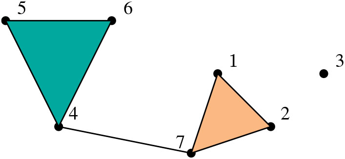
is a simplicial complex Reference Spanier[37]. Simplicial complexes can be represented using points, line segments, triangles, and simplices in higher dimensions, which may ease the understanding of the projections and the model (see Figure 1 for an illustration).
Illustration of a multivariate distribution in the dimension 7, knowing the marginal distribution
 $\{3\}$
, the bivariate projection
 $\{4,7\}$
, and the trivariate projections
 $\{1,2,7\}$
and
 $\{4,5,6\}$
. All subsets of these projections also correspond to known marginal distributions.

Definition 2.1. (Projective class.) Let
 ${\cal S} \in \mathcal{P}({\mathcal{D}})$
be decreasing. For a given characterizing function m, we say that a random vector
 ${{X}} \in
{\mathbb{R}}^{d}$
belongs to the projective class
 ${\cal
F}_{\mathcal{D}}({\cal S})$
if there exist some real coefficients
 $\alpha_{K,{\mathcal{D}}}$
,
 $K \subset {\mathcal{D}}$
, such that, for all
 ${{t}} \in \bar {\mathbb{R}}^d$
,
 \begin{equation}
m({{t}},{{X}}) = \sum_{K \in {\cal S}} \alpha_{K,{\mathcal{D}}}
m({{t}},{{X}}_K).
\label{eqn3}
\end{equation}
We note that if a random vector X belongs to the projective class
 ${\cal F}_{\mathcal{D}}({\cal S})$
then the set of suitable coefficients
 $\{\alpha_{K,{\mathcal{D}}}, K \subset \mathcal{D}\}$
satisfying (2.2) is not necessarily unique. Note also that if
 ${\mathcal{D}} \in {\cal S}$
, any d-dimensional random vector is in
 ${\cal F}_{\mathcal{D}}({\cal S})$
, using for example, constant coefficients
 $\alpha_{K,{\mathcal{D}}}$
equal to 1 if
 $K={\mathcal{D}}$
and equal to 0 otherwise. This is quite natural, since the class
 ${\cal
F}_{\mathcal{D}}({\cal S})$
intends to define multivariate distributions that can be fully determined by some of their projections. This is obviously the case when the initial joint distribution is already in
 ${\cal S}$
.
The projective class explicitly depends on the set
 ${\cal S}$
of given projections. It also depends implicitly on the choice of the characterizing function m, but for the sake of simplicity, it will not be indexed by m. A distribution (e.g. a centered Gaussian distribution) can be projective for a characterizing function
 $m_1$
(e.g. the logarithm of the characteristic function), but not for a characterizing function
 $m_2$
(e.g. the cumulative distribution function). At last, note that a priori, the coefficients
 $\alpha_{K,\mathcal{D}}$
may also depend on the choice of the characterizing function m, but for the sake of simplicity, they will not be indexed by m. We will show however that under some simple conditions, one can find coefficients that do not depend on the choice of m (see Remark 2.6).
It is not trivial to assess the compatibility conditions between arbitrary characterizing functions of the projections; given arbitrary
 $m({{t}},{{X}}_K)$
in (2.2), determining if the resulting m(t,X) indeed corresponds to a characterizing function is difficult. As an example, if m is a characteristic function, the verification may rely on known criteria such as Bochner’s theorem or multivariate extensions of Pólya’s theorem. If m is a transformation of a cumulative distribution function, the verification may rely on differentiation of this function using chain rule differentiation and multivariate extensions of Faa Di Bruno’s formula. For known projective families (see Section 3), the compatibility is ensured, but in practice (see Section 4) it may rely on some numerical verifications. As in Section 1, we refer to Reference Dall’aglio, Kotz and Salinetti[8], Reference Joe[21], and Reference Kellerer[24], for supplementary material on the question of projections compatibility.
2.2 Properties
In this subsection we discuss several properties of projective distributions regarding uniqueness, stability, and statistical inference. In particular, we provide explicit expressions for the coefficients appearing in Definition 1, in the case of fixed projections up to a given dimension.
Assuming that a distribution is projective, we give here a necessary and sufficient condition ensuring the uniqueness of the coefficients
 $\{\alpha_{K,\mathcal{D}}\}_{K \in {\cal S}}$
, which further implies that the distribution characterized by (2.2) is unique. The condition relies on the given projections
 $m({{t}}, {{X}}_K),\,K
\in {\cal S}$
.
Proposition 2.1. (Condition on the projections for uniqueness.) Define
 $S\,{:\!=}{\cal S}$
if
 $m_0\neq 0$
, and
 $S\,{:\!=}\,{\cal
S}\setminus\{\emptyset\}$
if
 $m_0=0$
. Consider a finite set of points
 $\mathcal{T} \subset \bar {\mathbb{R}}^d$
, and denote the matrix
 $M_{S}(\mathcal{T})\,{:\!=}\,(m({{t}}, {{X}}_K))_{{{t}} \in \mathcal{T},
K \in S}$
. Assume that the distribution of X is projective, and denote the vector of coefficients
 ${\boldsymbol\alpha} \,{:\!=}\,
(\alpha_{K,\mathcal{D}})_{K \in S}$
, then the following results hold.
(i) If there exists a set
$\mathcal{T}$
with
$|\mathcal{T}|=|S|$
such that the matrix
$M_{S}(\mathcal{T})$
is invertible, then
${\boldsymbol\alpha}$
is unique.(ii) If
${\boldsymbol\alpha}$
is unique then, for every set
$\mathcal{T}$
of distinct points with
$|\mathcal{T}|=|S|$
, the matrix
$M_{S}(\mathcal{T})$
is invertible.(iii) In particular, when
${\cal S}=\{K \subset {\mathcal{D}},\, |K|\le 2\}$
and
$m_0=0$
,
${\boldsymbol\alpha}$
is unique if there exists
${{t}}
\in \bar {\mathbb{R}}^d$
such that, for all
$K \in {\cal S}$
,
$m_K^*({{t}})=m({{t}}, {{X}}_K)-\smash{\sum_{J \subset K, J\neq
K}m({{t}}, {{X}}_{J})}>0$
.


Remark 2.4. The combination of (i) and (ii) above implies the following necessary and sufficient condition for uniqueness:
 ${\boldsymbol\alpha}$
is unique if and only if there exists a set
 $\mathcal{T}$
with
 $|\mathcal{T}|=|S|$
such that the matrix
 $M_{S}(\mathcal{T})$
is invertible.
Proof of Proposition 2.1. It is clear that if
 $m_0=0$
then
 $\alpha_{\emptyset,\mathcal{D}}m({{t}},
{{X}}_\emptyset)=0$
whatever the value of
 $\alpha_{\emptyset,\mathcal{D}}$
. Multiplied by zero, this coefficient has no impact, we thus exclude it from the analysis by setting
 $S={\cal S}\setminus\{\emptyset\}$
in the case when
 $m_0=0$
. Let us show (i). Write the vector
 ${{m}}_X(\mathcal{T})=(m({{t}}, X))_{{{t}} \in \mathcal{T}}$
. The main linear equality of (2.2) is
 \begin{equation}
{{m}}_X(\mathcal{T}) = M_{S}(\mathcal{T}) {\boldsymbol\alpha}
\label{eqn4}
\end{equation}
so that when
 $M_{S}(\mathcal{T})$
is invertible,
 ${\boldsymbol\alpha} = [
M_{S}(\mathcal{T})]^{-1}{{m}}_X(\mathcal{T}) $
is uniquely determined.
To prove (ii), consider a set
 $\mathcal{T}$
of distinct points with
 $|\mathcal{T}|=|S|$
. Again, (2.2) can be written as (2.3). This linear system of
 $|S|$
equations admits either no solution, which is excluded by the assumption that the distribution of X is projective, an infinite number of solutions, which is excluded by the assumption that
 ${\boldsymbol\alpha}$
is unique, or a unique solution, which is the only possible case. This implies, by the Rouché–Capelli theorem, that the rank of the matrix
 $M_{S}(\mathcal{T})$
is equal to
 $|S|$
, or, equivalently, that this matrix is invertible.
For (iii), write
 $S=\{K_1, \ldots, K_s\}$
, set
 ${{t}} \in \bar
{\mathbb{R}}^d,$
and set
 $\mathcal{T}=\{{{t}}_K, K \in S\}$
. Write P the matrix with components
 $P_{ij}=1$
if
 $K_i\subset K_j$
or 0 otherwise. We can check that the component i,j of the matrix
 $M_{S}(\mathcal{T})$
is
 \begin{equation*}
(M_{S}(\mathcal{T}))_{ij} = m({{t}}_{K_i}, {{X}}_{K_j})=
m({{t}}, {{X}}_{K_i \cap K_j}).
\end{equation*}
For any set L,
 $K=L$
if and only if K is a subset of L but not a strict subset of L; thus,
 $${({M_S}({\mathcal {T}}))_{ij}} = \sum\limits_{K \in S,{\kern 1pt} K \subset {K_i} \cap {K_j}} m (t,{X_K}) - \sum\limits_{K \in S,{\kern 1pt} K\mathop \subset \limits_ \ne {K_i} \cap {K_j}} m (t,{X_K}).$$
By assumption, for all
 $K\in {\cal S}$
,
 $|K|\le 2$
. The following equality holds for
 $|L|=1$
, since both the left- and right- hand terms are equal to 0 in this case. The equality also holds for
 $|L|=2$
, because on the right-hand side,
 $K \in S, J\subset K, J \neq K$
implies that
 $|J|=1$
and
 $|K|=2$
, and
 $K\subset L$
with
 $|K|=|L|=2$
implies that
 $K=L$
, i.e.
 $$\sum\limits_{K \in S,{\kern 1pt} K\mathop \subset \limits_ \ne L} m (t,{X_K}) = \sum\limits_{K \in S,{\kern 1pt} K \subset L} \; \;\sum\limits_{J \subset K,{\kern 1pt} J \ne K} m (t,{X_J}).$$
Finally, for
 $h\in \{1, \dots, s\}$
, as
 $K_h \subset K_i \cap K_j$
if and only if
 $P_{hi}P_{hj}=1$
,
 \begin{equation*}
(M_{S}(\mathcal{T}))_{ij} = \sum_{K_h \in S,\, K_h \subset K_i \cap K_j}
m_{K_h}^*({{t}})= \sum_{K_h \in S} {P}_{hi} \cdot m_{K_h}^*({{t}})
\cdot P_{hj}
\end{equation*}
so that
 $M_{S}(\mathcal{T})= {P}^\top D P$
, where D is the diagonal matrix with diagonal
 $\{m_K^*({{t}}),\, K \in S\}$
. When
 ${\cal S}=\{K
\subset {\mathcal{D}},\, |K|\le 2\}$
, up to a rearrangement, P is an upper triangular matrix with ones on its diagonal. Thus,
 $\det(P)=1$
and, finally,
 $\det(M_{S}(\mathcal{T}))=\det(D)$
. Under the assumption of (iii),
 $\det(D)>0$
and the result holds.
In the next proposition we prove the following projection stability property: if a random vector belongs to the class
 ${\cal
F}_{\mathcal{D}}({\cal S})$
then any subvector also belongs to
 ${\cal
F}_{\mathcal{D}}({\cal S})$
, and we compute the corresponding coefficients.
Proposition 2.2. (Projection stability.) Let X be a d-dimensional random vector in
 ${\cal
F}_{\mathcal{D}}({\cal S})$
, with associated coefficients
 $\{\alpha_{K,{\mathcal{D}}}, \, K\in {\cal S}\}$
. Then, for any nonempty
 $L \subset {\mathcal{D}}$
, the subvector
 ${{X}}_L$
belongs to
 ${\cal
F}_L({\cal S})$
, where for any nonempty subset J of L, a suitable set of associated coefficients is given by
 $${\alpha _\emptyset }_{,L} = \sum\limits_{K \subset D\backslash L,{\kern 1pt} K \in s} {{\alpha _{K,D}}} .$$
which implies, in particular, that
 $\alpha_{J, L}=0$
if
 $J\not\subset L$
.
Let
 $d_0$
be an integer such that
 $1\leq d_0\leq d$
. When
 ${\cal S}=\{K
\subset {\mathcal{D}},\, |K|\le d_0\}$
, and when the coefficients
 $\{\alpha_{J,L}, \, J \subset L\}$
depend only on the subsets cardinals, i.e.
 $\alpha_{J, L}=\alpha_{j, \ell}$
with
 $j =|{J}|\in \{1, \ldots,
d\}$
and
 $\ell =|{L}|\in \{0, \ldots, d\}$
, then a suitable set of associated coefficients is given by
 \begin{equation}
\alpha_{j,\ell} =\sum_{k=j}^{\min(d_0,d-\ell+j)} \binom{d-\ell}{k-j}
\alpha_{k,d} \quad\text{if } j \leq \min(\ell,d_0),
\label{eqn6}
\end{equation}
and
 $\alpha_{j,\ell}=0$
otherwise.
Proof. First note that, due to the second assumption on m(t,X), we have
 $m({{t}}, {{X}}_{K \cap L}) = m(P_{K \cap
L}{{t}},{{X}})= m(P_{K}P_L{{t}},{{X}})=
m(P_L{{t}},{{X}}_K)$
. Thus, using (2.2), we have
 \begin{align*}
m({{t}},{{X}}_L) &= m(P_L{{t}}, {{X}})
\\
&= \sum_{K \in {\cal S}} \alpha_{K,{\mathcal{D}}}
m(P_L{{t}},{{X}}_K)
\\
&= \sum_{K \in {\cal S}} \alpha_{K,{\mathcal{D}}} m({{t}},{{X}}_{K
\cap L})
\\
& = \sum_{J \subset L} \;\;\sum_{K \in {\cal S},\, K \cap L=J}
\alpha_{K,{\mathcal{D}}} m({{t}}, {{X}}_J) .
\end{align*}
By assumption,
 $K \in {\cal S}$
implies that
 $J=K \cap L \in {\cal S}$
. Setting
 $\alpha_{J, L} = \sum_{K \in {\cal S},\, K \cap L=J}
\alpha_{K,{\mathcal{D}}}$
as in (2.4), we finally obtain
 \begin{equation*}
m({{t}}, {{X}}_L) = \sum_{J \subset L,\, J \in {\cal S}} \alpha_{J,
L} m({{t}}, {{X}}_J);
\end{equation*}
hence,
 ${{X}}_L$
belongs to
 ${\cal F}_L( {\cal S})$
.
Finally, note that
 $K\cap L=J$
if and only if
 $J\subset L$
and
 $J\subset
K$
and
 $K\cap L\subset J$
. As a consequence, if
 $J \not \subset L$
, the sum in (2.4) is empty and
 $\alpha_{J,L}=0$
.
We now prove the second part of the proposition. When
 ${\cal S}=\{K
\subset {\mathcal{D}},\, |{K}|\leq d_0\}$
, we have, using (2.4),
 \begin{equation*}
\alpha_{J,L}= \sum_{K' \subset {\mathcal{D}}\setminus{L},\, |K'|\le
d_0-|J|} \alpha_{K' \cup J,{\mathcal{D}}}.
\end{equation*}
Now, let
 $j=|J|$
and
 $\ell=|L|$
. If
 $j > \ell$
, it is clear that
 $J \not
\subset L$
and
 $\alpha_{J,L}=0$
. As
 $K' \subset {\mathcal{D}} \setminus
L$
and
 $|K'|\le d_0-|J|$
, we get
 $0 \le |K'| \le \min(d_0-j,d-\ell)$
. Thus, when
 $J \subset L$
,
 \begin{equation*}
\alpha_{J, L} = \sum_{k=0}^{\min(d_0-j,d-\ell)} \sum_{K' \subset
{\mathcal{D}}\setminus{L},\, |K'|=k} \alpha_{K' \cup J,{\mathcal{D}}}
\end{equation*}
and if the coefficients
 $\alpha_{J,L}$
depend only on the cardinals,
 \begin{equation*}
\alpha_{j, \ell} = \sum_{k=0}^{\min(d_0-j,d-\ell)} \sum_{K' \subset
{\mathcal{D}}\setminus{L},\, |K'|=k} \alpha_{k+j,d}=
\sum_{k=0}^{\min(d_0-j,d-\ell)} \binom{d-\ell}{k} \alpha_{k+j,d},
\end{equation*}
yielding the second result.
Remark 2.5. (Case of
 $\emptyset$
) Note that
 $\emptyset$
necessarily belongs to
 ${\cal S}$
. In the case where
 $m({{t}},{{X}}_\emptyset) \neq 0$
, (2.2) may involve a constant
 $\alpha_{\emptyset,{\mathcal{D}}}$
, and implies that
 $\smash{\sum_{K \subset {\mathcal{D}}, K \in {\cal S}}
\alpha_{K,{\mathcal{D}}}}=1$
. In this case, it becomes useful to determine the coefficients
 $\alpha_{\emptyset,L}$
. For any nonempty L, (2.4) becomes
 $${\alpha _{\emptyset ,L}} = \sum\limits_{K \subset D\backslash L,{\kern 1pt} K \in S} {{\alpha _{K,D}}} .$$
When
 $L=\emptyset$
, (2.2) remains valid for
 $\mathcal{D}=\emptyset$
if one defines
 $\alpha_{\emptyset,\emptyset}=1$
.
As previously noted, the coefficients
 $\alpha_{K,\mathcal{D}}$
and
 $\alpha_{\emptyset, L}$
may depend on the choice of the characterizing function m. However, one can check that using
 $\tilde m(t,{{X}}) = c
m(t,{{X}})$
for a positive constant c leads to
 $\tilde
m(t,{{X}}_\emptyset) = c m(t,{{X}}_\emptyset)$
and to unchanged coefficients
 $\tilde \alpha_{K,\mathcal{D}}= \alpha_{K,\mathcal{D}}$
.
Corollary 2.1. (Given projections up to dimension
 $d_0$
.) Let X be a d-dimensional random vector in
 ${\cal
F}_{\mathcal{D}}({\cal S})$
. Assume that all projections of X are given up to a dimension
 $d_0$
, so that
 ${\cal S}=\{K \subset
{\mathcal{D}},\, |{K}|\leq d_0\}$
. Assume that the associated coefficients
 $\{\alpha_{J,L}, \, J \subset L\}$
depend only on the subsets cardinals, i.e.
 $\alpha_{J, L}=\alpha_{j, \ell}$
with
 $j
=|{J}|\in \{1, \ldots, d\}$
and
 $\ell =|{L}|\in \{0, \ldots, d\}$
. Assume, furthermore, that
 $\alpha_{k,k}=1$
for all
 $k \le d_0$
. Then the coefficients
 $\alpha_{d_0-z, d}$
can be obtained recursively, using
 \begin{equation}
\alpha_{d_0-z,d} =1 - \sum_{i=1}^z \binom{d-d_0+z}{i} \alpha_{i+d_0-z,d}
\label{eqn7}
\end{equation}
for
 $z=1, \ldots, d_0$
, starting with
 $\alpha_{d_0,d}=1$
. In particular for
 $2 \le d_0 \le d$
, we get
 $\alpha_{d_0,d}=1$
,
 $\alpha_{d_0-1,d}\,{=}\,{-}\,(d-d_0)$
,
 $\alpha_{d_0\,{-}\,2,d} \,{=}\, 1 +
\smash{\tfrac12}{(d-d_0+2)}(d-d_0-1)$
.
When
 $d_0 \ge 3$
,
 $\alpha_{d_0-3,d} = 1 -
(d-d_0+3)\lbrace1-\smash{\tfrac12}{(d-d_0+2)}(1-\smash{\tfrac13}{(d-d_0+1)})\rbrace$
. For higher orders, one can check by induction that these coefficients do depend only on
 $d-d_0$
, but their expression is omitted here.
Proof. Under the assumption that
 $\alpha_{k,k}=1$
for all
 $k \le d_0$
, this follows directly from Proposition 2.2, by writing (2.5) in the case where
 $j=\ell \le d_0$
, and setting
 $i=k-j$
,
 $j=d_0-z$
. We obtain
 $\alpha_{d_0,d}=1$
when
 $z=0$
, and (2.6) when
 $z\ge 1$
.
Remark 2.6. (Explicit coefficients.) The fact that
 $\alpha_{k,k}=1$
for all
 $k\leq d_0$
means that if we are given a k-dimensional marginal, we do not try to retrieve it from the given lower-dimensional marginals. Under this assumption, and under the assumption that the coefficients in the projective decomposition depend only on the subsets cardinals, the previous corollary provides a set of suitable coefficients
 $\{\alpha_{j,\ell}\}$
which are explicitly given, independently of the choice of m.
The case where all bivariate projections are given is a very natural and interesting case. In practical applications, bivariate projections can be graphically visualized, and the estimation of the dependence structure among each pair of random variables is still tractable. The following remark shows that in this case, under some simple conditions, the coefficients
 $\alpha_{J,L}$
can be computed explicitly.
Remark 2.7. (Given bivariate projections.) Consider the same assumptions as in Corollary 2.1 and assume that all bivariate projections of a multivariate distribution are given, so that
 $d_0=2$
and
 ${\cal S}=\{J \subset {\mathcal{D}}, |{J}|\leq 2\}$
. Then, for all nonempty
 $L \subset {\mathcal{D}}$
, we can reformulate (2.2) as
 \begin{equation}
m({{t}},{{X}}_L) = \alpha_{0,|L|} m_0 -(|L|-2) \sum_{J \subset L,\,
|J|=1} m({{t}}, {{X}}_J) + \sum_{J \subset L,\, |J|=2} m({{t}},
{{X}}_J),
\label{eqn8}
\end{equation}
where
 $\alpha_{0,0}=1$
,
 $\alpha_{0,\ell} = 1 + \smash{\tfrac{1}{2}}\ell(\ell-3)$
,
 $\ell \ge 1$
and where
 $m_0=m({{t}},{{X}}_\emptyset)$
is defined in Remark 2.1.
Let
 ${{X}} \in {\mathbb{R}}^d$
be a random vector in
 ${\cal
F}_{\mathcal{D}}({\cal S})$
. Since
 ${\mathcal{D}}=\{1,\dots,d\}$
is a finite set, the set of subsets of
 ${\mathcal{D}}$
is also finite, and we can define the following matrix, indexed by the subsets of
 ${\mathcal{D}}$
:
 \begin{align}
A=(\alpha_{J,L})_{J \subset {\mathcal{D}}, L \subset {\mathcal{D}}}.
\label{eqn9}
\end{align}
We will write
 $A_{.,L}$
for the column vector relative to the subset L.
Proposition 2.3. The coefficients in the matrix A satisfy the following constraints.
(i) If the set of associated coefficients
$\{\alpha_{J,L}\}$
is unique then the matrix A defined in (2.8) is idempotent, i.e.
$A^2=A$
.(ii) If, furthermore, the coefficients depend only on the subset’s cardinal, i.e.
$\alpha_{J,L}=\alpha_{j,\ell}$
with
$j=|J|$
and
$\ell=|L|$
, we obtain, for
$0 \le j \le \ell \le d$
, Now define
$${\alpha _{j,\ell }} = \sum\limits_{k = j}^{\min ({d_0},\ell )} {\left( \matrix{
\ell - j \cr
k - j \cr} \right)} {\alpha _{j,k}}{\alpha _{k,\ell }}.$$
${s}_{j,\ell}\,{:\!=} \smash{\binom{\ell-2}{j-2} \alpha_{j,\ell}}$
when
$j\ge 2$
. When
$j \ge 2$
, the above equation becomes
$${s_{j,\ell }} = \sum\limits_{k = j}^{\min ({d_0},\ell )} {{s_{j,k}}} {s_{k,\ell }}.$$
Proof. Let
$L \subset {\mathcal{D}},\,|L|\ge 1$
.


From Proposition 2.2,
 \begin{equation*}
m({{t}},{{X}}_L) = \sum_{K \subset L, K \in {\cal S}}\alpha_{K, L}
m({{t}},{{X}}_K).
\end{equation*}
From Proposition 2.2, we also have
 $m({{t}},{{X}}_K)= \smash{\sum_{J \subset K, J \in {\cal S}}
\alpha_{J,K}m({{t}},{{X}}_J)}$
, so that, finally,
 \begin{align*}
m({{t}},{{X}}_L) &=\sum_{K \subset L, K \in {\cal S}} \;\;\sum_{J
\subset K, J \in {\cal S}} \alpha_{J, K} \alpha_{K, L}
m({{t}},{{X}}_J)
\\
&=\sum_{J \subset L, J \in {\cal S}} \;\;\sum_{K \subset L, K \in {\cal
S}} \alpha_{J, K} \alpha_{K, L} m({{t}},{{X}}_J)
\end{align*}
as
 $\alpha_{J, K}=0$
if
 $J \not \subset K$
. Then, for all t,
 \begin{equation*}
m({{t}},{{X}}_L) = \sum_{J \subset L, J \in {\cal S}} \bigg\{
\sum_{K \subset L, K \in {\cal S}} \alpha_{J, K} \alpha_{K, L}\bigg\}
m({{t}},{{X}}_J)
\end{equation*}
so that, using the uniqueness of the set of coefficients
 $\{\alpha_{J,L}\},$
 \begin{align*}
\alpha_{J,L} = \sum_{K \subset L, K \in {\cal S}} \alpha_{J, K}
\alpha_{K, L}
\end{align*}
and, thus, A is idempotent.
Let us now focus on the second part of the proposition. For a subset
 $L\subset {\mathcal{D}}$
with cardinal
 $\ell$
and
 $k\leq \ell$
, define
 $[L]^k\,{:\!=} \{K\subset L \text{ such that } |K|=k\}$
. Assume that when
 $K
\subset L$
the coefficients
 $\alpha_{K,L}$
depend only on the cardinals
 $k=|K|$
and
 $\ell=|L|$
of the considered sets, and assume that
 $\alpha_{K,L}=0$
if
 $K \notin {\cal S}$
, i.e.
 $\alpha_{k,\ell}=0$
if
 $k
> d_0$
. Then
 \begin{align*}
m(t,{{X}}_L) &= \sum_{K\subset L} \alpha_{K,L}m(t,{{X}}_K)
\\
&= \sum_{k=0}^{\min(d_0, \ell)} \alpha_{k,\ell} \sum_{K \in [L]^k}
m(t,{{X}}_K)
\\
&=\sum_{k=0}^{\min(d_0, \ell)} \alpha_{k,\ell} \sum_{K \in [L]^k}
\bigg\{\sum_{j=0}^{\min(d_0, k)} \alpha_{j,k} \sum_{J \in [K]^j}
m(t,{{X}}_J)\bigg\}.
\end{align*}
Note that, by a simple combinatorial argument, for
 $j \le k$
,
 $$\sum\limits_{K \in {{[L]}^k}} {\sum\limits_{J \in {{[K]}^j}} m } (t,{X_J}) = \left( \matrix{
\ell - j \cr
k - j \cr} \right)\sum\limits_{J \in {{[L]}^j}} m (t,{X_J}),$$
which entails that
 \begin{align*}
m({{t}},{{X}}_L) = \sum_{k=0}^{\min(d_0, \ell)}
\sum_{j=0}^{\min(d_0, k)} \alpha_{k,\ell}\alpha_{j,k}\binom{\ell-j}{k-j}
\sum_{J \in [L]^j} m({{t}},{{X}}_J).
\end{align*}
On the other hand, we have
 \begin{align*}
m({{t}},{{X}}_L) = \sum_{j=0}^{\min(d_0, \ell)} \alpha_{j,\ell}
\sum_{J \in [L]^j} m({{t}},{{X}}_J)
\end{align*}
so that, for all t, for all
 $j \le k$
,
 \begin{align*}
\alpha_{j,\ell} = \sum_{k=j}^{\min(d_0, \ell)} \binom{\ell-j}{k-j}
\alpha_{j,k} \alpha_{k,\ell};
\end{align*}
thus, the second result holds.
Remark 2.8. Note that, due to the projection stability property of Proposition 2.2, any column of the matrix A can be deduced from the last column by multiplication by a matrix with values in
 $\{0,1\},$
i.e.
 $A_{\cdot,L} = \smash{P^{(L)}} A_{\cdot,{\mathcal{D}}}$
, where the
 $2^d \times 2^d$
matrix
 $\smash{P^{(L)}}$
is defined by its components
 \begin{align*}
P^{(L)}_{J,K} =
\begin{cases}
1 & \text{if } J=K\cap L \text{ and } K \in {\cal S},
\\
0 & \text{otherwise,}
\end{cases}
\end{align*}
for J, K, L subsets of
 ${\mathcal{D}}$
. Indeed, we have from Proposition 2.2,
 \begin{equation*}
\alpha_{J, L} = \sum_{K \in {\cal S}, K \cap L=J}
\alpha_{K,{\mathcal{D}}} = \sum_{K \in {\cal S}} P^{(L)}_{J,K}
\alpha_{K,{\mathcal{D}}}.
\end{equation*}
Let us finish this section with a useful property of our construction for statistical inference. Assume that we have at our disposal an independent and identically distributed sequence
 $({{X}}_1, \dots, {{X}}_n)$
, where, for each i,
 ${{X}}_i \in {\mathbb{R}}^d$
. The following proposition highlights the fact that if we have estimators with good properties for the distribution of subvectors
 ${{X}}_K$
, then these properties are maintained for the estimator of the distribution of the whole vector X.
As in Definition 2.1, let
 ${\cal S} \in
\mathcal{P}({\mathcal{D}})$
be decreasing. For any K in
 ${\cal S}$
, assume that we can construct an estimator
 $\widehat m_n({{t}}, X_K)$
of
 $m({{t}}, X_K)$
using the sample
 $({{X}}_1, \dots, {{X}}_n)$
for
 ${{t}} \in {\mathbb{R}}^d$
. From (2.2), a natural expression for an estimator
 $\widehat m_n({{t}},{{X}})$
of the distribution of the whole vector X is given by
 \begin{align}
\widehat m_n({{t}},{{X}}) = \sum_{K \in {\cal S}}
\alpha_{K,{\mathcal{D}}} \, \widehat m_n({{t}},{{X}}_K).
\label{eqn10}
\end{align}
Proposition 2.4. (Unbiasedness and consistency.) The natural estimator given by (2.9) preserves unbiasedness and consistency.
(i) If, for each K,
$\widehat m_n({{t}},{{X}}_K)$
is unbiased then
$\widehat m_n({{t}},{{X}})$
is also unbiased.(ii) If, for each K,
$\widehat m_n({{t}},{{X}}_K)$
is consistent then
$\widehat m_n({{t}},{{X}})$
is also consistent.


Proof. Property (i) is obvious by the linearity in (2.2) and the linearity of expectation.
To prove property (ii), first suppose that, for each K,
 $\widehat
m_n({{t}},{{X}}_K)$
converges in probability to
 $m({{t}},{{X}}_K)$
as n goes to
 $\infty.$
By Slutsky’s theorem, the vector
 ${({\hat m_n}(t,{X_K}))_{K \in S}}$
converges in probability to
 ${(m(t,{X_K}))_{K \in S}}$
, and by the continuous mapping theorem, any linear combination of elements of
 ${({\hat m_n}(t,{X_K}))_{K \in S}}$
converges in probability to the same linear combination of elements of
 ${(m(t,{X_K}))_{K \in S}}$
, which is the desired result. Notice that we are able to use Slutsky’s theorem, which is a statement about convergence in distribution, because all the limits are towards real constant values.
Remark 2.9. If a central limit theorem (CLT) is available for each
 $\widehat
m_n({{t}},{{X}}_K)$
, then further work is needed to obtain a CLT for
 $\widehat m_n({{t}},{{X}})$
defined in (2.9). Indeed for
 $K_1, K_2 \in {\cal S}$
,
 $K_1\cap K_2$
is not necessarily empty, which implies that the elements in the linear combination (2.9) are dependent. A CLT for
 $\widehat
m_n({{t}},{{X}})$
is thus determined by the strength of this dependence.
3 Examples
3.1 Elliptical random vectors
Recall from Reference Joe[21] that d-dimensional elliptical distributions are characterized by the fact that their characteristic function can be written in the following form: for any
 ${{t}} \in {\mathbb{R}}^d$
,
 \begin{equation*}
{\mathbb{E}}[{{\mathrm{e}}^{i {{t}}^\top ({{X}}-{\boldsymbol\mu})}}] = \phi
({{t}}^\top \Sigma {{t}} )
\end{equation*}
for a given function
 $\phi\colon {\mathbb{R}}_+ \rightarrow {\mathbb{R}}$
which is called the generator of the distribution, where
 ${\boldsymbol\mu}$
is the mean of the vector X and
 $\Sigma$
is a nonnegative definite matrix. We assume here that the generator
 $\phi$
does not depend on the dimension d of the random vector, i.e. that the elliptical distribution is consistent in the sense of Reference Kano[23].
One interesting feature of families of elliptical distributions is that they allow heavy tails, while preserving some advantageous properties of multivariate Gaussian distributions. Indeed, an elliptical distribution has a stochastic representation as a product of two independent random elements: a univariate radial distribution and a uniform distribution on an ellipsoid (see Chapter 2 of Reference Fang, Kotz and Ng[12]). This representation makes possible the analysis of the density functions, the moments, the conditional distributions, the symmetries, and the infinite-divisibility properties of elliptical distributions (see Reference Frahm[13]). Other than multivariate Gaussians, elliptical distributions include the student t-distributions, the symmetric generalized hyperbolic distribution, the power exponential distributions, and the sub-Gaussian
 $\alpha$
-stable distributions among others. Families of elliptical distributions are widely applied in statistics, in particular, in the area of robust statistics, as a starting point for the development of the M-estimates of multivariate location and scale (see Chapter 2 of Reference Maronna, Martin and Yohai[28]). It is also a rather standard family of distributions in financial modelling: see Reference Frahm, Junker and Szimayer[14] and the references therein. Thus, constructing a distribution with given multivariate elliptical marginals is a useful and interesting problem, which we explore in this subsection.
Let us first remark that, for a given generator
 $\phi$
, when one considers a centered multivariate elliptical distribution, the distribution is fully characterized by all components
 $\sigma_{ij}$
of the matrix
 $\Sigma$
, that is, by all bivariate elliptical projections of the distribution (it does not mean that the multivariate elliptical distribution is the only one having those projections).
It is thus quite natural to analyse, in the case of elliptical distributions, the links between the matrix
 $\Sigma$
and a given set of submatrices
 $\Sigma_{K_1}, \ldots, \Sigma_{K_n}$
for
 $K_1, \ldots, K_n$
subsets of
 ${\mathcal{D}}=\{1, \ldots, d\}$
. This is easier to do using the matrix
 $\Sigma$
rather than its inverse
 $\Sigma^{-1}$
. It thus seems easier to work with characteristic functions or entropy (which are expressed using
 $\Sigma$
) rather than densities or cumulative distribution functions (which are expressed using
 $\Sigma^{-1}$
).
We will try to express the quantity
 ${{t}}^\top \Sigma {{t}}$
as a linear combination of products
 ${{t}}_K^\top \Sigma_{K} {{t}}_K$
, where K belongs to known projection indexes in
 ${\cal S}$
.
Definition 3.1. (
 ${\cal S}$
-admissible sequence.) Let
 ${\mathcal{D}} \subset {\mathbb{N}}$
, and let
 ${\cal S}$
be a decreasing subset of
 ${\mathcal{D}}$
. A sequence of coefficients
 $\alpha_{K,{\mathcal{D}}}$
,
 $K \in {\cal S}$
, is said to be
 ${\cal
S}$
-admissible if, for all matrix
 $\Sigma$
, for all t,
 \begin{equation}
{{t}}^\top \Sigma {{t}} = \sum_{K \subset {\mathcal{D}}, K \in
{\cal S}} \alpha_{K,{\mathcal{D}}} \cdot {{t}}_K^\top \Sigma_{K}
{{t}}_K,
\label{eqn11}
\end{equation}
where
 $\Sigma_{K}$
is the submatrix of
 $\Sigma$
with indices in K.
The following lemma provides a characterization of such coefficients.
Lemma 3.1. (Characterization of
 ${\cal S}$
-admissible sequence.) Let
 $d_0\in {\mathbb{N}}$
be such that
 $2 \le d_0 \le d$
, and assume that
 ${\cal S}=\{K \subset {\mathcal{D}},\, |K|\le d_0\}$
. Assume, furthermore, that, for any sets
 $K, {\mathcal{D}}$
,
 $\alpha_{K,
{\mathcal{D}}}=\alpha_{|K|, |{\mathcal{D}}|}$
. A sequence
 ${\boldsymbol\alpha}_d=(\alpha_{k,d})_{k \le d}$
of coefficients is
 ${\cal S}$
-admissible if and only if it can be written
 \begin{equation}
\alpha_{1,d}= -\sum_{k=2}^{d_0} {s}_k \frac{d-k}{k-1}
\quad\text{and}\quad \alpha_{k,d}= {{s}_k}\bigg/{\binom{d-2}{k-2}}, \qquad
k=2, \ldots, d_0,
\label{eqn12}
\end{equation}
for some real values
 ${s}_2, \cdots, {s}_{d_0}$
such that
 ${s}_2+\ldots+{s}_{d_0} = 1$
.
In the particular case where the coefficients are deduced from only two given dimensions, i.e. if there exists
 $k_0\geq 2$
such that
 ${s}_i=0$
whenever
 $i \notin \{1,k_0\}$
, we get a particular
 ${\cal S}$
-admissible sequence
 $${\alpha _{1,d}} = - {{d - {k_0}} \over {{k_0} - 1}}\quad {\rm{and}}\quad {\alpha _{k,d}} = {1 \over {\left( \matrix{
d - 2 \cr
{k_0} - 2 \cr} \right)}}\quad {\rm{if}}\;k = {k_0}\;{\rm{and }}{\alpha _{k,d}} = 0{\rm{ otherwise, }}k = 2, \ldots ,{d_0}.$$
Furthermore, when
 $d_0=2$
, the only
 ${\cal S}$
-admissible sequence is
 $${\alpha _{1,d}} = - (d - 2)\quad {\rm{and}}\quad {\alpha _{2,d}} = 1.$$
Proof. Assume that
 ${\boldsymbol\alpha}_{d}$
is
 ${\cal S}$
-admissible, and that
 $\alpha_{K,{\mathcal{D}}}$
depend only on
 $|K|$
and
 $|{\mathcal{D}}|$
. Let
 $$({i_0},{j_0}) \in {{\mathcal{D}}^2}$$
,
 $i_0\neq j_0$
. Isolating the coefficient
 $\smash{{{{t}}_{i_0}\Sigma_{i_0, j_0} {{t}}_{j_0}}}$
on both sides of (3.1), we obtain
 $$1 = \sum\limits_{k = 2}^{{d_0}} | \{ K:K \subset ,|K| = k,\{ {i_0},{j_0}\} \subset K\} |{\alpha _{k,d}} = \sum\limits_{k = 2}^{{d_0}} {\left( \matrix{
d - 2 \cr
k - 2 \cr} \right)} {\alpha _{k,d}}.$$
Denoting
 ${s}_k= \alpha_{k,d} \smash{\binom{d-2}{k-2}}$
for all k, we obtain
 $\smash{\sum_{k=2}^{d_0} {s}_k }= 1$
. Now considering the coefficient
 $\smash{{{{t}}_{i_0}\Sigma_{i_0, i_0} {{t}}_{i_0}}}$
on both sides of (3.1), we obtain
 \begin{equation*}
1= \sum_{k=1}^{d_0}\alpha_{k,d} |{\{K\colon K \subset {\mathcal{D}},
|K|=k,\, i_0 \in K}\}| = \alpha_{1,d} + \sum_{k=2}^{d_0}
\binom{d-1}{k-1}\alpha_{k,d}.
\end{equation*}
Now as
 ${s}_k= \alpha_{k,d} \smash{\binom{d-2}{k-2}}$
for all k,
 \begin{equation*}
1 =\alpha_{1,d} + \sum_{k=2}^{d_0}{s}_k \frac{\binom{d-1}{k-1}}
{\binom{d-2}{k-2}}=\alpha_{1,d} + \sum_{k=2}^{d_0}{s}_k \frac{d-1}{k-1}.
\end{equation*}
Finally, using
 $1=\smash{\sum_{k=2}^{d_0} {s}_k}$
, (3.2) holds. The remainder of the proof follows by a direct application of this last equation.
A direct application of such an
 ${\cal S}$
-admissible sequence is given in the following proposition. As a consequence, the further defined distance to admissibility (see subsection 4.1) is always 0 for elliptical distributions.
Proposition 3.1. (Elliptical distributions are projective.) Consider a d-dimensional random vector X having elliptical distribution with mean
 ${\boldsymbol\mu}$
, matrix
 $\Sigma,$
and invertible generator
 $\phi$
. Let
 ${\mathcal{D}}=\{1, \ldots, d\}$
and
 $[{\mathcal{D}}]^k=\{K \subset {\mathcal{D}},\, |K|=k\}$
. Consider that all projections are given up to a dimension
 $d_0$
,
 $2 \le d_0 \le d$
, so that
 ${\cal S}=\{K \subset {\mathcal{D}},\, |K|\le d_0\}$
. Then, for any
 ${\cal S}$
-admissible sequence
 ${\boldsymbol\alpha}_d=(\alpha_{1,d},
\ldots, \alpha_{d_0,d})$
,
 $$\phi ({t^{\rm{T}}}\Sigma t) = \phi (\sum\limits_{k = 1}^{{d_0}} {{\alpha _{k,d}}} \sum\limits_{K \in {{[{\mathcal {D}}]}^k}} {t_K^{\rm{T}}} {\Sigma _K}{t_K})$$
holds, where
 $\Sigma_{K}$
is the submatrix of
 $\Sigma$
with indices in K. In other words, setting
 $m({{t}},{{X}})= \phi^{-1} \smash{(
{\mathbb{E}}[{{\mathrm{e}}^{i {{t}}^\top ({{X}}-{\boldsymbol\mu})}}] )}$
and
 ${\cal
S}=\{K \subset {\mathcal{D}}, |K|\le 2\}$
, we have
 $$X \in {\rm{ }}{{\mathcal {F}}_D}(S).$$
In particular, when
 $d_0=2$
(i.e. starting from all bivariate projections), the admissible sequence is
 $\alpha_{1,d}=-(d-2)$
and
 $\alpha_{2,d}=1$
.
Proof. By definition, for any
 ${\cal S}$
-admissible sequence,
 ${{t}}^\top
\Sigma {{t}}\! =\! \smash{\sum_{k=1}^{d_0} \alpha_{k,d}} \smash{\sum_{K
\in [{\mathcal{D}}]^k} {{t}}_K^\top \Sigma_{{K}}} {{t}}_K$
. One can also check that the functions m are suitable characterizing functions satisfying Assumption 2.1 with
 $a=0$
and
 $m_0=\phi^{-1}(1)=0$
; hence, the result.
Remark 3.1. (Matrix A in the elliptical case
 $d_0=2$
.) Consider the elliptical case with
 $d_0=2$
. Then we get, by Lemma 3.1,
 \begin{align*}
\alpha_{J,L} =
\begin{cases}
0 & \text{if } J \not\subset L,
\\
- (|L|-2) & \text{if } |J|=1 \text{ and } J \subset L,
\\
1 & \text{if } |J|=2 \text{ and } J \subset L.
\end{cases}
\end{align*}
In particular, if
 $d=3$
and
 ${\mathcal{D}}=\{1,2,3\}$
, the matrix
 $A=(\alpha_{J,L})_{J \subset {\mathcal{D}}, L \subset {\mathcal{D}}}$
is
 $$A = \left( {\matrix{
1 & 0 & 0 & 0 & 0 & 0 & { - 1} \cr
0 & 1 & 0 & 0 & 0 & 0 & { - 1} \cr
0 & 0 & 1 & 0 & 0 & 0 & { - 1} \cr
0 & 0 & 0 & 1 & 0 & 0 & 1 \cr
0 & 0 & 0 & 0 & 1 & 0 & 1 \cr
0 & 0 & 0 & 0 & 0 & 1 & 1 \cr
0 & 0 & 0 & 0 & 0 & 0 & 0 \cr
} } \right),$$
where the seven rows and columns correspond to successive subsets of
 ${\mathcal{D}}$
:
 \begin{equation*}
\{1\},\, \{2\},\, \{3\},\, \{1,2\},\, \{1,3\},\, \{2,3\},\, \{1,2,3\}.
\end{equation*}
As
 $m_0=0$
in the elliptical case, it is not necessary to compute the coefficients
 $\alpha_{J,L}$
for
 $J=\emptyset$
or
 $L=\emptyset$
(see Remark 2.5). One can easily check that we can apply Proposition 2.3 to deduce that A is idempotent, which can also be verified by hand in this example.
Consider a centered elliptical random vector with zero mean and covariance matrix
 $\Sigma$
. As seen before, its distribution is thus projective, so that, for all
 ${{t}} \in {\mathbb{R}}^d$
,
 \begin{equation}
{{t}}^\top \Sigma {{t}} = \sum_{K \subset {\mathcal{D}},\, K \in
{\cal S}} \alpha_{K,{\mathcal{D}}} \cdot {{t}}_K^\top \Sigma_{K}
{{t}}_K,
\label{eqn14}
\end{equation}
Let us denote by
 $D_K$
the
 $d\times d$
diagonal matrix having 1s only at indices in K. We can write
 $${t^{\rm{T}}}\Sigma t = {t^{\rm{T}}}(\sum\limits_{K \subset D,{\kern 1pt} K \in S} {{\alpha _{K,D}}} {({D_K})^{\rm{T}}}\Sigma {D_K})t$$
so that this holds for all t if and only if
 $$\Sigma = \sum\limits_{K \subset D,{\kern 1pt} K \in S} {{\alpha _{K,D}}} {\rm{Ex}}{{\rm{t}}_D}({\Sigma _K}),$$
where
 ${\mathrm{Ext}_{{\mathcal{D}}}}(\Sigma_K)$
is the extension of the matrix
 $\Sigma_K$
to the dimension
 $d \times d$
, i.e. the matrix having components
 $${({\Sigma _K})_{ij}}$$
for all
 ${({E_K})_{ij}}$
and 0 when
 $i \not \in
K$
or
 $j \not \in K$
. Now assume that, for all
 $K \in {\cal S}$
, we have a given estimator
 $\widehat \Sigma_K$
of the covariance matrix of
 ${{X}}_K$
. From the previous equation, a natural estimator of the full covariance matrix
 $\Sigma$
is defined as
 $$\hat \Sigma {\mkern 1mu} : = \sum\limits_{K \subset D,K \in S} {{\alpha _{K,D}}} {\rm{Ex}}{{\rm{t}}_D}({\hat \Sigma _K}).$$
Now assume that classical estimators
 $\widehat \Sigma_K$
are also available for any
 $K \subset {\mathcal{D}} $
, then we get the following result: if, for all
 $K \in {\cal S}$
,
 $\widehat \Sigma_K$
is the submatrix of
 $\widehat \Sigma_{{\mathcal{D}}}$
for indices in K then
 \begin{equation*}
\widehat \Sigma =\widehat \Sigma_{{\mathcal{D}}}.
\end{equation*}
This can be checked using (3.4), when choosing t the vector having 0 everywhere except for two given components i and j.
In particular, consider for example a centered Gaussian random vector, if
 $\widehat \Sigma_K$
are maximum likelihood estimators,
 $K \subset
{\mathcal{D}}$
, it is well known that they are directly proportional to the sample covariance matrix, so that all
 $\widehat \Sigma_K$
are submatrices of
 $\widehat \Sigma_{{\mathcal{D}}}$
, and, thus,
 $\widehat
\Sigma= \widehat \Sigma_{{\mathcal{D}}}$
. This also holds for many shrinkage estimators. On the contrary, when
 $\widehat \Sigma_K$
are built by inverting an estimated precision matrix,
 $\widehat
\Sigma_{{\mathcal{D}}}$
and
 $\widehat \Sigma$
may differ. The study of all possible estimators of
 $\Sigma$
is however outside of the scope of the present paper.
When the generator
 $\phi$
is unknown, another interesting perspective is to use the underlying linearity of the projective class in order to build a nonparametric estimator of
 $\phi$
.
3.2 Vectors built from bivariate distributions
Assume that a family
 $${({\mu _{i,j}})_{(i,j) \in {D^2}}}$$
of probability measures on
 ${\mathbb{R}}^2$
is given, for some nonnegative parameters
 $\theta_{i}$
,
 $\theta_{j},$
and
 $\theta_{i,j}$
specific to each couple
 $$(i,j) \in {D^2}$$
, and that each
 $\mu_{i,j}$
satisfies
 \begin{align}
\mu_{i,j}((t,+\infty), (u,+\infty))\,{:\!=} \psi(\theta_{i}t + \theta_{j}u +
\theta_{i,j} t u), \qquad (t,u) \in {\mathbb{R}}_+^2,
\label{eqn15}
\end{align}
where
 $\psi$
is a given appropriate function.
Thanks to our previous results, we can construct a random variable X, with values in
 ${\mathbb{R}}_+^d$
, such that the survival function of each subvector
 $(X_i,X_j)$
is given by the right-hand side of (3.5).
Let us first analyze the copula function associated to
 $(X_i,X_j)$
. To do so, assume that
 $\psi$
is a decreasing bijection from
 ${\mathbb{R}}_+$
to (0,1] such that
 $\psi(0)=1$
and that derivatives of
 $\psi$
exist up to the order d. Denote by
 $\psi^{-1}$
the inverse function of
 $\psi$
. Let
 $t=(t_i,t_j) \in {\mathbb{R}}_+^2$
and
 $S_{ij}(t)= \psi(\theta_i t_i +
\theta_j t_j + \theta_{ij} t_i t_j)$
. The one-dimensional survival functions are then given by
 $S_{i}(t)= \psi(\theta_i t_i)$
from which we obtain
 $\theta_i t_i= \psi^{-1}(S_{i}(t))$
, so that finally
 \begin{equation*}
S_{ij}(t)= \psi\bigg(\psi^{-1}(S_{i}(t)) + \psi^{-1}(S_{j}(t)) +
\frac{\theta_{ij}}{\theta_i\theta_j} \psi^{-1}(S_{i}(t))
\psi^{-1}(S_{j}(t))\bigg).
\end{equation*}
Therefore, we can write
 \begin{equation*}
S_{ij}(t)= C_{S_{ij}}(S_{i}(t), S_{j}(t)),
\end{equation*}
where the survival copula
 $C_{S_{ij}}$
is given by
 \begin{equation}
C_{S_{ij}}(u,v)= \psi\bigg(\psi^{-1}(u)+ \psi^{-1}(v) +
\frac{\theta_{ij}}{\theta_i\theta_j} \psi^{-1}(u) \psi^{-1}(v)\bigg),
\qquad (u,v) \in [0,1]^2.
\label{eqn16}
\end{equation}
Example 3.1. Examples of survival functions in the form of (3.5), or (3.7) in the d-dimensional case, include the following particular cases.
(i) If
$\psi(x)=\exp({-}\,x)$
then
$3.6$
reduces to which is the survival copula associated with Gumbel’s bivariate exponential distribution (see [31, Copula (4.2.9)]).
\begin{equation*}
C_{S_{ij}}(u_i, u_j) = u_i u_j \exp\bigg({-}\,\frac{\theta_{ij}}
{\theta_i\theta_j} \ln u_i \ln u_j \bigg),
\end{equation*}
(ii) In the case where
$\theta_{i,j}=0$
for every
$$(i,j) \in {D^2}$$
and if the generator
$\psi$
is d-monotone (see Definition 3.2), we obtain a survival copula which is Archimedean with generator
$\psi$
. It is clear that in this specific case, the multivariate distribution in a higher dimension will still have an Archimedean survival copula with the same generator, as it will appear further in (3.7).(iii) In the case where
$\theta_{i,j}=0$
for every
$$(i,j) \in {D^2}$$
and all the coefficients
$\theta_i$
are equal, we obtain the class of Schur constant vectors, studied for example in Reference Nelsen[32]. In that case, the function
$\psi$
corresponds to the generator of the Schur constant vector, which has an Archimedean survival copula in the bivariate case, whose generator is given by
$\psi^{-1}$
.


Let us now explicitly construct a distribution on
 ${\mathbb{R}}_+^d$
, with the given bivariate marginals. Given the form
 $3.5$
of these marginals, we choose the following characterizing function:
 \begin{equation*}
m({{t}},{{X}})= \psi^{-1} \left( {\mathbb{P}}[{X_i>t_i,\, i \in
{\mathcal{D}}} ]\right).
\end{equation*}
With the assumptions we made for
 $\psi$
, it is clear that the function m satisfies Assumption 2.1, with constant
 $a=+\infty$
and
 $m_0=m({{t}},\emptyset)=0$
. The function m is thus a suitable characterizing function.
Now consider the decreasing set
 ${\cal S}=\{ J \subset {\mathcal{D}},\,
|J|\le 2\}$
, and assume that m belongs to the class
 ${\cal
F}_{\mathcal{D}}({\cal S})$
in Definition 2.1: each multivariate distribution is assumed here to depend only on its bivariate projections. Assume furthermore that the associated coefficients
 $\alpha_{J,K}$
in Definition 2.1,
 $J\subset K$
, depend only on cardinals
 $j=|J|$
and
 $k=|K|$
, so that
 $\alpha_{J,K}=\alpha_{j, k}$
.
Due to Remark 2.7, if a valid multivariate distribution belongs to the class
 ${\cal F}_{\mathcal{D}}({\cal S})$
then its survival function must take the form
 \begin{equation*}
\skew4\bar F_K({{t}})=\psi \biggl({-}\,(k-2) \sum_{J \subset K, |J|=1}
m({{t}}, {{X}}_J) + \sum_{J \subset K, |J|=2} m({{t}},
{{X}}_J) \biggr).
\end{equation*}
Note that
 $m(t,{{X}}_{\{i}\})=\theta_{i}t_i $
and
 $m(t,{{X}}_{\{i,j}\})=\theta_{i}t_i + \theta_{j}t_j+ \theta_{i,j} t_i
t_j$
. Now using
 $\sum_{\{i,j\} \subset K}( \theta_{i}t_i + \theta_{j}t_j)
=(k-1) \sum_{\{i\} \subset K} \theta_{i}t_i,$
we obtain
 \begin{equation}
\skew4\bar F_K({{t}}) = \psi\biggl( \sum_{\{i\} \subset K} \theta_{i}t_i +
\sum_{\{i,j\} \subset K} \theta_{i,j} t_i t_j \biggr).
\label{eqn17}
\end{equation}
Proposition 3.2 below shows that under some sufficient conditions this expression is a proper multivariate survival function. This proposition makes use of the following definition of d-monotony, as given in Reference McNeil and Nešlehová[30].
Definition 3.2. (d-monotone function.) A real function f is called
 $d-$
monotone in (a, b), where
 $a, b \in
\bar {\mathbb{R}}$
and
 $d \geq 2$
, if it is differentiable there up to the order
 $d - 2$
and the derivatives satisfy
 \begin{equation*}
({-}\,1)^k f^{(k)}(x) \geq 0, \qquad k = 0, 1, \ldots , d-2,
\end{equation*}
for any
 $x \in (a, b)$
and further if
 $\smash{({-}\,1)^{d-2}f^{(d-2)}}$
is nonincreasing and convex in (a, b). For
 $d = 1$
, f is called 1-monotone in (a, b) if it is nonnegative and nonincreasing over
 $(a,
b)$
.
Proposition 3.2. The following three conditions ensure that, for any fixed subset K of size
 $k\,{:\!=}|K|$
,
 $\skew4\bar F_K({{t}})$
is a proper multivariate survival function:
(i)
$\psi$
and its derivatives goes fast enough to zero: for every
$n\leq
k-1$
,
${\lim_{x \rightarrow +\infty} x \psi^{(n)}(x) = 0 }$
;(ii)
$\psi$
is k-monotone;(iii) for all distinct i, j in K,
$\theta_{i,j} \in [0, \; \theta_i
\theta_j \rho_{\psi, k}]$
,where
$$
\rho_{\psi,k}= \inf\limits_{x \in {\mathbb{R}}^+,\, {{r}} \le k/2,\,
{{r}} \textrm{~odd}} \gamma_{k,{{r}}}^{-1}
\bigg|{\frac{\psi^{(k+1-{{r}})}(x)}{\psi^{(k-{{r}})}(x)}}\bigg|
\quad\text{and}\quad
\gamma_{k,{{r}}}=\frac{1}{{{r}}}\binom{k-2{{r}}+2}{2}.
$$


For example, if
 $|K|=k=3$
and
 $\psi(x)=\exp({-}\,x)$
, then
 $\psi$
is a k-monotone function satisfying condition (i) and (ii). It also satisfies (iii) with coefficient
 $\rho_{\psi,k}=\smash{\tfrac{1}{3}}$
, and the function
 $\skew4\bar F_K$
defined in (3.7) is a valid multivariate survival function if
 $\theta_{i,j} \le \theta_i
\theta_j /3$
for all
 $i,j \in K$
.
Proof. We have
 \begin{equation*}
\skew4\bar F_K({{t}}) = \psi\biggl( \sum_{\{i\} \subset K} \theta_{i}t_i +
\sum_{\{i,j\} \subset K} \theta_{i,j} t_i t_j \biggr) =\psi (
Q({{t}})),
\end{equation*}
with
 \begin{equation*}
Q({{t}})= \sum_{\{i\} \subset K} \theta_{i}t_i + \sum_{\{i,j\} \subset
K} \theta_{i,j} t_i t_j .
\end{equation*}
Let us consider without loss of generality
 $K=\{1, \ldots, k\}$
and
 ${{t}}=(t_1, \ldots, t_k)$
. Let us define
 \begin{equation*}
f_K({{t}}) = ({-}\,1)^k {\frac{\partial^k}{\partial t_1 \cdots \partial
t_k}} \skew4\bar F_K({{t}}).
\end{equation*}
If
 $f_K$
is a nonnegative function whose integral is 1, then it will be the density of a random vector, and
 $\skew4\bar F_K({{t}})$
will be a proper multivariate CDF.
Positivity. Let us first establish conditions under which
 $f_K$
is a nonnegative function. The multivariate Faa Di Bruno’s formula gives us
 \begin{equation}
f_K({{t}}) = ({-}\,1)^k \sum_{\pi\in\Pi_K} \psi^{(\left|\pi\right|)}
(Q({{t}}))\cdot\prod_{B\in\pi}
{\frac{\partial^{\left|B\right|}Q({{t}})}{\prod_{j\in B} \partial
t_j}},
\label{eqn18}
\end{equation}
where
 $\Pi_K$
is the set of all partitions of K,
 $B\in \pi$
means that B runs through all nonempty blocks of a considered partition
 $\pi$
. In the following, we will write
 ${{\partial^2 Q({{t}})}/{\partial
{{t}}_B}} = {{\partial Q({{t}})}/{\partial t_i \partial t_j}} $
and
 $\theta_B=\theta_{i,j}$
, where
 $B=\{i,j\}$
.
Note that
 $\partial^{\left|B\right|}Q({{t}})$
is 0 when
 $|B|\ge 3$
. Thus, the only partitions
 $\pi$
involved in the calculation contain blocks of 1 or 2 elements only. Hereafter, we denote by
 $\Pi_K^{{r}}$
the partitions in
 $\Pi_K$
that contain exactly r distinct blocks of size 2. For a partition
 $\pi \in \Pi_K^{{r}}$
, these r blocks will be denoted by
 $B_1^\pi, \ldots, B_{{r}}^\pi$
. Such a partition
 $\pi \in \Pi_K^{{r}}$
contains r blocks of size 2 and
 $k-2{{r}}$
blocks of size 1, so that
 $|\pi|=k-{{r}}$
. Thus, we obtain (with the convention
 $\smash{\prod_{i=1}^0 }= 1$
)
 \begin{equation*}
f_K({{t}}) = ({-}\,1)^k \sum_{{{r}}=0}^{\lfloor k/2 \rfloor} \sum_{\pi \in
\Pi_K^{{r}}} \psi^{(k - {{r}})}(Q({{t}})) \cdot \prod_{i=1}^{{r}}
{\frac{\partial^{2}Q({{t}})}{\partial {{t}}_{B_i^\pi}}} \prod_{j\in
K\setminus \cup_i B_i^\pi}{\frac{\partial Q({{t}})}{\partial t_j}}.
\end{equation*}
If
 $\psi$
is k-monotone,
 $\psi^{(k - {{r}})}=({-}\,1)^{k-{{r}}}
|{\psi^{({k} - {{r}})}}|$
, and setting
 $\mathcal{N}_k= \{0, \ldots,
\lfloor k/2 \rfloor\}$
,
 \begin{equation*}
f_K({{t}}) = \sum_{{{r}} \in \mathcal{N}_k} \sum_{\pi \in \Pi_K^{{r}}}
|{\psi^{(k - {{r}})}(Q({{t}}))}| \cdot \prod_{i=1}^{{r}}
\left({-}\,{\frac{\partial^{2}Q({{t}})}{\partial
{{t}}_{B_i^\pi}}}\right)\prod_{j\in K\setminus \cup_i
B_i^\pi}{\frac{\partial Q({{t}})}{ \partial t_j}} .
\end{equation*}
We can write
 $f_K({{t}})=\sum_{{{r}} \in \mathcal{N}_k} \xi({{r}})$
. Assume that all
 $\theta_i\ge 0$
and
 $\theta_{i,j}\ge 0$
,
 $i,j\in K$
. Under this assumption, we can check that, when r is even,
 $\xi({{r}})\ge 0$
. As a consequence,
 \begin{equation*}
\sum_{{{r}} \in \mathcal{N}_k} \xi({{r}}) \ge \sum_{{{r}} \in
\mathcal{N}_k, {{r}} \textrm{~odd}} [ \xi({{r}}) + \xi({{r}}-1)].
\end{equation*}
Let us try to simplify
 $\xi({{r}}) + \xi({{r}}-1)$
. First remark that, for
 ${{r}}\ge 1$
,
 \begin{align*}
|\Pi_K^{{r}}| = \binom{k}{2}\cdots\binom{k-2({{r}}-1)}{2}\bigg/{{r}}!=
\frac{2^{-{{r}}}{k!}}{{(k-2{{r}})!\,{{r}}!}}
\end{align*}
and
 $\smash{|\Pi_K^{{r}}|=\gamma_{k,{{r}}}|\Pi_K^{{{r}}-1}|}$
, with
 $\gamma_{k,{{r}}}=\smash{({1}/{{{r}}})\binom{k-2{{r}}+2}{2}}$
.
Let us write
 $\xi({{r}})=\smash{\sum_{\pi \in \Pi_K^{{r}}} z(B_1, \ldots,
B_{{{r}}}^\pi)}$
. The term
 $\xi({{r}}-1)$
can be written as
 \begin{equation*}
\sum_{\pi \in \Pi_K^{{{r}}-1}} z(B_1^\pi,\ldots, B_{{{r}}-1}^\pi) =
\gamma^{-1}_{k,{{r}}} \sum_{\pi \in \Pi_K^{{r}}} z(B_1^\pi,\ldots,
B_{{{r}}-1}^\pi),
\end{equation*}
and, thus,
 \begin{equation*}
\xi({{r}})+\xi({{r}}-1)= \sum_{\pi \in \Pi_K^{{r}}} [ z(B_1^\pi, \ldots,
B_{{{r}}}^\pi) - \gamma^{-1}_{k,{{r}}} z(B_1^\pi, \ldots,
B_{{{r}}-1}^\pi) ].
\end{equation*}
As a consequence, a sufficient condition to ensure that
 $f_K({{t}})
\ge 0$
is that, for any
 $B=\{i,j\}$
, any odd r, and any t,
 \begin{equation*}
-{\frac{\partial^{2}Q({{t}})}{\partial {{{t}}_{B_i}}}}|{\psi^{(k -
{{r}})}(Q({{t}}))}| + \gamma^{-1}_{k,{{r}}} |{\psi^{(k + 1 -
{{r}})}(Q({{t}}))}| {\frac{\partial Q({{t}})}{\partial
t_i}}{\frac{\partial Q({{t}})}{\partial t_j}} \ge 0.
\end{equation*}
Thus yielding the sufficient condition to ensure the positivity of
 $f_K(x)$
.
Absolute continuity. Let us now check if the integral of
 $f_K$
is summing to 1. If so,
 $\skew4\bar F_K$
would be a valid absolutely continuous distribution, without a singular component. First assume that, for all integers
 $n \le k-1$
,
 \begin{equation*}
\lim\limits_{x \rightarrow +\infty} x \psi^{(n)}(x) = 0.
\end{equation*}
Recall that
 $\smash{\skew4\bar F_K({{u}})}= \psi(Q(u_1, \ldots, u_k))$
. We now make use of the multivariate Faa Di Bruno’s formula as in (3.8). Seen as a function of
 $u_n$
, the derivative of
 $\smash{\skew4\bar F_K({{u}})}$
with respect to
 $u_{n+1},
\ldots, u_k$
can be written as a sum of terms
 $\smash{\psi^{(i)}}(a u_n +
b) P(u_n)$
, where P is a polynomial of degree at most 1 and a,b some real values. Thus, under assumption (i), for any
 ${{u}} \in
{\mathbb{R}}^k$
and all integers
 $n \le k-1$
,
 \begin{equation*}
\lim\limits_{u_n \rightarrow +\infty} \frac{\partial^{k-n}} {\partial
u_{n+1} \cdots \partial u_k} \skew4\bar F_K({{u}}) = 0.
\end{equation*}
As a consequence, we can show by recursion that in this case,
 \begin{equation*}
\skew4\bar F_K(t_1, \ldots, t_k) = \int_{t_1}^{+\infty} \cdots
\int_{t_k}^{+\infty} \frac{\partial^k}{\partial u_1 \cdots \partial u_k}
\skew4\bar F_K(u_1, \ldots, u_k) {\,\mathrm{d}} u_k \cdots {\,\mathrm{d}} u_1.
\end{equation*}
Using the fact that
 $\smash{\skew4\bar F_K(0, \ldots, 0)}=1$
, we conclude that the derivative function
 $f_K$
is nonnegative and is integrating to 1 on the whole domain
 ${\mathbb{R}}_+^{k}$
. Under chosen assumptions, it thus defines a proper probability measure and
 $\skew4\bar F_K$
is a valid multivariate survival function.
4 Practical implementation
4.1 Distance to admissibility
We have seen several examples of projective distributions that can be used in practice, as elliptically contoured distributions or distributions satisfying (3.7). In the following, we show that the method is also applicable in situations where the data does not necessarily come from a projective distribution.
In practice, it can naturally happen that the multivariate distribution of a considered data is not projective. In such a case, the resulting multivariate function F, obtained from the characterizing function and from multivariate projections by (2.2), may not be a proper CDF. However, by construction, this function has exactly the prescribed multivariate margins.
It is quite a usual problem that estimators do not always satisfy all the required constraints. Among many examples include an empirical copula is not a copula Reference Erdely and González-Barrios[11], some Kaplan–Meier estimated distributions are defective Reference Portnoy[33], some estimated quantiles do not satisfy monotonicity Reference Chernozhukov, Fernández-Val and Galichon[5], some nested copulas do not satisfy C-measure positivity on all hyperrectangles Reference Hofert and Pham[17], Reference McNeil[29], etc. Here the obtained F, even when it is increasing on each component, may not satisfy the positivity of its cross derivatives. In this section we approximate the function F that we obtain by an admissible CDF.
We show hereafter that, even in the case where the resulting function F is not a CDF, we can find a proper CDF
 $F^+$
that is close to F in some sense and such that its projections are close to the prescribed ones. Furthermore, we will see in numerical illustrations that the maximal distance between F and
 $F^+$
can be easily estimated, and that it is very small in some considered applications.
In the following we denote
 $[{-{\infty}}, {x}]=\{(s_1, \ldots,
s_d)\colon s_1\le x_1, \ldots, s_d \le x_d\}$
for any vector
 ${x}=(x_1, \ldots, x_d) \in {\mathbb{R}}^d$
.
Proposition 4.1. (Maximal admissibility distance.) Let
 ${\mathcal{D}} \subset {\mathbb{R}}^d$
and denote
 ${\mathcal{D}}_{x}= {\mathcal{D}} \cap [{-{\infty}}, {x}]$
. Consider a function
 $F\colon {\mathcal{D}} \rightarrow [0,1]$
, and assume that there exists a function
 $f\colon {\mathbb{R}}^d \rightarrow {\mathbb{R}}$
such that, for any
 ${x} \in {\mathcal{D}}$
,
 $F({x})={\int_{{\mathcal{D}}_{x}} f({s})}{\,\mathrm{d}}{s}$
. Assume, furthermore, that
 $\smash{\int_{{\mathcal{D}}}f({s})}{\,\mathrm{d}}{s}=1$
. Denote
 ${\mathcal{D}}^-=\{{s} \in {\mathcal{D}}, f({s}) \lt 0\}$
and
 $\Delta=\smash{\int_{D^-} |{f({s})}| }{\,\mathrm{d}}{s}$
. Then there exists a function
 $F^+\colon {\mathcal{D}} \rightarrow [0,1]$
such that
(i)
$F^+\colon {\mathcal{D}} \rightarrow [0,1]$
is a proper multivariate CDF;(ii)
$d_{{\mathrm{KS}}}(F,F^+)\le {\Delta}/{(1+\Delta)}$
;(iii) for any
$K \subset \{1, \ldots, d\}$
,
$d_{{\mathrm{KS}}}(F_K,F^+_K) \le
{\Delta}/{(1+\Delta)}$
,where
$F_K({x})=F(P_K {x})$
,
$F^+_K({x})=F^+(P_K {x}),$
and
$P_K {x} = (p_1, \ldots, p_d),$
with
$p_i= x_i$
if
$i \in K$
,
$p_i=+\infty$
otherwise, as defined in (2.1). Here
$d_{{\mathrm{KS}}}(F,G)=\sup_{{x} \in {\mathcal{D}}} |{F({x})-G({x})}|$
denotes the Kolmogorov–Smirnov distance between two functions F and G. Such a function
$F^+$
is given by where
$$
F^+({x}) = \int_{{\mathcal{D}}_{x}} f^+({x}){\,\mathrm{d}}{x},
$$
$f^+({x})=({1}/{(1+\Delta)})f({x})$
if
${x} \in
{\mathcal{D}} \setminus {\mathcal{D}}^-$
and
$f^+({x})=0$
otherwise.


Proof. Let
 $F^+({x}) = \smash{\int_{{\mathcal{D}}_{x}} f^+({x})}{\,\mathrm{d}}{x},$
where
 $f^+$
is defined in the proposition, and let
 ${\mathcal{D}}^+\,{:\!=} {\mathcal{D}}
\setminus {\mathcal{D}}^-$
for simplicity. First,
 $f^+$
is nonnegative and using
 $\smash{\int_{\mathcal{D}} f( {x})} {\,\mathrm{d}}{x}=1$
, we obtain
 $\smash{\int_{{\mathcal{D}}^+} f^+({x})} {\,\mathrm{d}}{x} =1$
, so that
 $f^+$
is a proper PDF and (i) holds.
When
 $\Delta>0$
, define
 $\alpha({x}) \in [0,1]$
by
 \begin{align*}
\alpha({x}) \,{:\!=} \frac{\int_{{\mathcal{D}}_{x} \cap
{\mathcal{D}}^-} |{f({x})}| {\,\mathrm{d}}{x}}{\int_{{\mathcal{D}}^-}
|{f({x})}|{\,\mathrm{d}}{x}}.
\end{align*}
and
 $\alpha({x})=0$
otherwise. Note that
 $\alpha({x})$
is such that
 $\smash{\int_{{\mathcal{D}}_{x} \cap {\mathcal{D}}^-} f({x})} {\,\mathrm{d}}{x} = -\alpha(x) \Delta$
, and
 \begin{align*}
F^+({x})=\frac{1}{1+\Delta}\int_{D_{x} \cap {\mathcal{D}}^+}
f({x}) {\,\mathrm{d}}{x} = \frac{1}{1+\Delta}\left(\int_{D_{x} } f({x}){\,\mathrm{d}}{x} - \int_{D_{x} \cap {\mathcal{D}}^-} f({x}) {\,\mathrm{d}}{x} \right).
\end{align*}
From this, we obtain
 $F({x})-F^+({x}) = ({\Delta}/{(1+\Delta)}) (
F({x}) - \alpha({x}) )$
. As
 $\sup_{{x} \in {\mathcal{D}}} |
F({x}) - \alpha({x}) | \le 1,$
(ii) holds for this specific function
 $F^+$
.
As (ii) holds,
 $|{F({x})-F^+({x})}|\le {\Delta}/{(1+\Delta)}$
for any
 ${x} \in D$
, and, in particular, for any
 ${x}'=P_K {x}$
, so that (iii) holds.
Note that
 $\Delta=\smash{\int_{D^-} |{f({s})}|} {\,\mathrm{d}}{s}= -
\smash{\int_{D^-} f({s})} {\,\mathrm{d}}{s} = -(1-\smash{\int_{D^+} f({s})} {\,\mathrm{d}}{s})=\smash{\int_{D^+} f({s})} {\,\mathrm{d}}{s}-1$
, so that
 $\smash{\int_{D^+} f({s})} {\,\mathrm{d}}{s}=1+\Delta$
. As a consequence, we can define the failure ratio
 \begin{equation}
R = \frac{\int_{D^-} |{f({s})}| {\,\mathrm{d}}{s}}{\int_{D^+} |{f({s})}|
{\,\mathrm{d}}{s}} = \frac{\Delta}{1+\Delta},
\label{eqn19}
\end{equation}
which bounds the errors in Proposition 4.1. This ratio can easily be estimated by a discrete approximation of each integral, using classical techniques which avoid any normalization of the integrals.
In the case where
 $m({{t}},X)= \varphi \circ F({{t}}),$
where
 $\varphi$
is a bijection from (0,1] to
 ${\mathbb{R}}^+$
, we obtain
 \begin{equation*}
F_L({{t}}_L) = \varphi^{-1} \bigg(\sum_{J \subset L, J \in {\cal S}}
\alpha_{J,L} \cdot \varphi \circ F_J({{t}}_J)\bigg).
\end{equation*}
In this case if
 $\varphi$
,
 $\varphi^{-1}$
and all given projections
 $F_K$
are differentiable up to a sufficient order, then applying chain differentiation rules and multivariate Faa Di Bruno’s formula, we can show that F satisfies the assumptions of Proposition 4.1.
We note that, in practice, depending on the application, and when
 $\Delta$
is small, we may use F instead of
 $F^+$
, as the expression of F does not require computation of an integral. In particular, some sampling procedures like MCMC may be easily adapted to the function F instead of
 $F^+$
. In the latter case, the produced sample has by definition a valid multivariate CDF.
4.2 Numerical illustration on a real data set
In the following we give an example on a real data set. First, we illustrate a natural fit procedure on a trivariate data, by adjusting each marginal distribution, and then each copula. Second, we show that the proposed construction allows us to build a valid trivariate cumulative distribution with projections close enough to each of the prescribed ones.
4.2.1 Marginals and copulas fit
The purpose here is to provide reasonable univariate and bivariate fits using standard tools, without distorting the data, in order to illustrate the flexibility of our result and its applicability to some usual data. Surely, better fits can be proposed, but are outside the scope of the present paper.
We have obtained best univariate fits using classical existing tools in R software, and in particular the package fitdistrplus. Best copulas were obtained by the package VineCopula.
We present here the results obtained for the data LifeCycleSavings from the standard R software library datasets. We have used the first three columns of this data. We do not detail the data here, as the purpose here is just to build a parametric fit on a multivariate data, with given projections.
The marginal fits obtained for the considered data are gathered in Figure 2. One can see that, independently of our method, the fits with usual tools may be sensitive to multimodality of the data. The copula fit illustrations are presented in Figure 3. All univariate and bivariate fits are summarized in Table 1.
Univariate margins fits: empirical CDF (discontinuous line) and fitted CDF (continuous line) obtained by
 $\textsf{R}$
software package
 $\textsf{fitdistrplus}$
.

Copula fits: pseudo observations scatterplot and heatmap of the copula log-density, obtained by
 $\textsf{R}$
software package
 $\textsf{VineCopula}$
.

Fits obtained for the considered dataset, obtained by  $\textsf{R}$ software packages
 $\textsf{fitdistrplus}$ and
 $\textsf{VineCopula}$. Parametric expressions of the fits are those indicated in these packages.

Concerning both the CDF and the copulas, they exhibit quite different shapes, as it usually happens on many datasets. It thus seems particularly challenging to propose a trivariate function having exactly those fitted univariate and bivariate margins. In the next paragraph we show how to build such a function, using the method proposed in this paper.
4.2.2 Trivariate fit with prescribed bivariate projections
For more flexibility, we consider here a one-parameter class of characterizing functions, in the sense of Definition 2.1. As the given bivariate fits rely here on copulas, it is easier to deal with multivariate CDF or survival functions. The considered class is a parametric transformation of multivariate CDF:
 $$(t,{X_L}) = {\varphi _\theta }[{F_{{X_L}}}({t_L})].$$
For the link function
 $\varphi_\theta$
, we have chosen some parametric monotone functions such that
 $\varphi_\theta (1)=0$
, detailed hereafter. We can check that in this case
 $m_0=m({{t}},{{X}}_\emptyset)=\varphi_\theta
(F_{{{X}}}(+\infty, \ldots, +\infty)) = 0$
as defined in Remark 2.1. Using the proposed method and the result in Remark 2.7, when
 $|L|=3$
and with
 ${{t}}_L \in
{\mathbb{R}}^3$
, we obtain a fitted trivariate function, denoted
 ${F_{\theta}}$
,
 $${F_\theta }({t_L}) = \varphi _\theta ^{ - 1}[ - (|L| - 2)\sum\limits_{J \subset L,|J| = 1} {{\varphi _\theta }} ({F_{{X_J}}}({t_J})) + \sum\limits_{J \subset L,|J| = 2} {{\varphi _\theta }} ({F_{{X_J}}}({t_J}))].$$
Note that for some specific link functions and margins, theoretically valid distributions with this shape are given in Proposition 3.2.
As it was easier to use classical expressions with known parametric inverse functions, we have used specific link functions
 $\varphi_\theta$
. We have considered strictly positive and decreasing functions
 $\varphi_\theta \colon [0,1] \rightarrow {\mathbb{R}}^+$
of Table 4.1 of Reference Nelsen[31], that are also known to be Archimedean generators. We have tried the six first strict generators of [31, Table 4.1] (respectively, Clayton, AMH, Gumbel, Frank, Joe, and Hougaard generators). Then, we have selected the generator and its parameter that was minimizing the estimation of the failure ratio
 $R={\Delta}/{(1+\Delta)}$
in (4.1). The parameter
 $\theta$
is thus used to reduce the maximal distance between the obtained function
 ${F_{\theta}}$
and a proper multivariate CDF
 ${F_{\theta}}^+$
, as detailed in Proposition 4.1. We also compared the trivariate function
 ${F_{\theta}}$
and the empirical trivariate CDF
 $F_{\mathrm{emp}}$
of the data, by computing the average absolute error
 $\delta = ({1}/{n}) \smash{\sum_{i=1}^n |{{F_{\theta}}({x}_i)-{F_{\mathrm{emp}}}({x}_i)}|}$
, where
 ${x}_1, \ldots, {x}_n$
are the points in the dataset. In Figure 4 we show the different values of the estimated failure ratio R and the distance
 $\delta$
with the empirical CDF. The ratio R was estimated by replacing the integrals by sums over a regular grid of 1000 points between minimal and maximal values of each component of the dataset. Whereas the average absolute error
 $\delta$
is quite stable on this data, the failure ratio R is sensitive to the choice of the parameter
 $\theta$
. We verify hereafter that the results are not too sensitive to the grid used for the estimation.
Estimated failure ratio R (solid line) and distance
 $\delta$
to empirical CDF (dashed line), as a function of the parameter
 $\theta$
.

Finally, the results for this dataset, using the Hougaard generator
 $\varphi_\theta$
given by (4.2.9) in Table 4.1 of Reference Nelsen[31], are gathered in the following table:

For the estimation of R, using a more precise grid of 64000 points, in the extended domain
 $[0.9{{m}},1.1{M}],$
where m and M are the componentwise minimum and maximum of the points in the data, we obtained quite similar results, i.e. an estimated R equal to
 $0.000\,984$
at
 $\theta= 0.766$
. Notice that it is usual that some compatibility conditions can only be verified numerically over a grid of points; see [21, p.75].
We can check that the estimated admissibility of the fitted function
 ${F_{\theta}}$
is very good so that, in practice, as we can see in Figures 5 and 6, it may be unnecessary to compute the proper CDF
 ${F_{\theta}}^+$
of Proposition 4.1. Indeed, the numerical approximations involved by numerical differentiation or integration may be greater to the maximal distance
 $\Delta$
and the failure ratio
 $R\le \Delta$
.
Values of the fitted function
 ${F_{\theta}}$
(solid line) and the empirical CDF
 ${F_{\mathrm{emp}}}$
(dotted line), on several points of a diagonal line
 ${{m}} + a ({M}-{{m}})$
in
 ${\mathbb{R}}^3$
, as a function of the abscissa a.

Level curves of the fitted function
 ${F_{\theta}}$
(left panel) and the empirical CDF
 ${F_{\mathrm{emp}}}$
(right panel), on several points of the diagonal plane
 $ {{m}} + a ({A}-{{m}})+ b({B}-{{m}})$
, as a function of the abscissa a and the ordinate b (right panel).

Values of the fitted function on given bivariate projections correspond exactly, by construction, to the prescribed ones so that it is useless to draw these values. We can instead compute the values of the fitted function for a set of points belonging to a one-dimensional or a two-dimensional diagonal hyperplane. The considered data has 3 columns. For each column i in
 $\{1,2,3\}$
, denote
 $m_i$
the minimal observed value in this column, over all observations, and
 $M_i$
the maximal observed value. Let
 ${{m}}=(m_1, m_2, m_3)$
and
 ${M}=(M_1,M_2,M_3)$
(so that the cube [m,M] contains all observations of the dataset). Let us also define the two points
 $A=(M_1,m_2,M_3)$
and
 $B=(m_1,M_2,M_3)$
.
Suppose that the true distribution of the data set is given by the law of a vector
 $${\rm{(X\_1, X\_2, X\_3),}}$$
and suppose that we are interested in estimating the CDF of the univariate random variable
 $$
Z\,{:\!=}\max\biggl(\frac{X_1-m_1}{M_1-m_1}, \frac{X_2-m_2}{M_2-m_2},
\frac{X_3-m_3}{M_3-m_3}\biggr).
$$
In Figure 5 we have drawn the estimated CDF of Z coming from our construction and using
 ${\mathbb{P}}[{Z \le a}]= {\mathbb{P}}[{X_1 \le
m_1+a(M_1-m_1),\ldots, X_3 \le m_3+a(M_3-m_3)}]$
. More precisely, the figure shows the values of the function
 ${F_{\theta}}$
that we constructed, evaluated at several points of a diagonal
 ${{m}} + a
({M} - {{m}})$
, for different values of a. Despite that the fit is not perfect compared to the empirical values (the fits of the bivariate projections in Figure 2 were not perfect either), we observe that the estimated univariate CDF behaves normally (starting from 0 up to 1 and increasing).
Along the same lines, on the right panel of Figure 6, we have drawn values of the fitted function
 ${F_{\theta}}$
for points belonging to a plane
 ${{m}} + a ({A}-{{m}})+ b ({B}-{{m}})$
, for different values of a and b (left panel), the empirical counterpart is also drawn (right panel).
We can check that, again, the fitted function behaves normally and is increasing over each component. The admissibility problem can arise even for functions increasing on each components, with values in [0,1], as this requirement is not sufficient to define a CDF having positive cross derivatives.
At last, we have conducted the same analysis on other datasets of the R Software library datasets. Results are gathered in Table 3. For some datasets (stackloss, rock), the estimated values of R are not negligible and more investigations are needed, i.e. change in the bivariate projections, in the one-parameter link function
 $\varphi_\theta,$
or in the characterizing function m. For other datasets, we obtain very good numerical results, with sometimes estimated ratios R of order
 $10^{-6}$
, and the MathAchieve dataset also leads to a very good global fit of the trivariate distribution. In our experiments we did not use the (tedious) parametric expressions of the bivariate projections density, but instead some numerical differentiation. As a result, the distance between the proper CDF
 $F^+$
in Proposition 4.1 and the obtained fitted function would probably be comparable to the numerical errors induced by the numerical differentiation, so that we did not build this proper CDF. We have presented here a detailed procedure for a specific one-parameter class of characterizing functions. Introducing more parameters would logically result in smaller ratios R.
Final estimated failure ratio R and distance  $\delta$ to empirical for different datasets or for different considered columns. Results are sorted by estimated ratio R. Details of each bivariate fit are omitted here. The horizontal dashed lines highlight the previously detailed case study. The horizontal plain line separates the cases with estimated failure ratio greater than
 $0.05$.

The proposed method cannot guarantee that the final fitted multivariate function F does not correspond to a signed measure. However, as a conclusion of this numerical investigation, the following advantages are of practical utility.
• The obtained fitted distribution has exactly the prescribed projections, by construction.
• The Kolmogorov–Smirnov distance between the final fitted function and a proper CDF is bounded by a quantity R that can be estimated, and is small in our experiments. Thus, the fitted function can be directly used for many practical applications.
• One can build a proper CDF from the final fitted function. In such a case, the projections of this proper CDF are at maximal distance R from the prescribed ones.
5 Conclusion
In this paper wee have considered specific multivariate distributions, belonging to a class which was called projective. They rely on a linear link between some functional of the considered distribution and their multivariate margins. The choice of a linear link is not as restrictive as one would initially imagine, since it covers a variety of classical distributions from elliptical distributions to some natural survival models, as presented in Section 3.
In theory, for these distributions the compatibility between given multivariate margins and multivariate distribution is automatically ensured, by definition, and the coefficients linking multivariate margins with the whole distribution are easily obtained using, for example, Proposition 2.2, (2.6), and (2.7).
In practice, when dealing with a given dataset, one possibility is to use class projective distributions, as those described in Section 3 (elliptical distributions, specific survival model, etc.), and estimate its parameters. This way fitted projections are necessarily compatible with each other, and the admissibility is ensured for the resulting multivariate construction having prescribed projections. However, the fitted projections are then modeled by the same parametric family of functions.
Another possibility is to assume the validity of the linearity assumption for some characterizing functions belonging to a set of functions, as described in Section 4. In this case, given a data, fitted multivariate marginals, and a chosen characterizing function m, the coefficients and the expression of the candidate function for the whole multivariate distribution are easily obtained. This allows a huge variety of fitted projections. It remains to verify whether the fitted function with prescribed projections is a valid distribution, as done theoretically in Section 3.2 (but it involves many chain rule differentiations) or numerically in Section 4.2. In the latter case, it is always possible to build a proper multivariate CDF while controlling the distance to the prescribed projections, as detailed in Section 4.1.
At last, other characterizing functions can be tried, eventually relying on several parameters. This way one can theoretically build new classes of projective distributions, or try to satisfy, at least numerically, the validity of the fitted functions on some data.
Acknowledgements
This paper was written when the authors visited the Vietnam Institute for Advanced Study in Mathematics (VIASM). The authors warmly thank the VIASM institute for support. The authors are very grateful to the anonymous reviewers, the associate editor, and the editor for their careful reading and their many insightful comments and suggestions.