3.1. The experimental environment

We design a group experiment with a between-subject design. Each experimental session involves a fixed group of six subjects tasked with making point forecasts of output and inflation gaps in the next period. The experimental economy unfolds for 75 periods split into two separate subsessions, one of 40 and one of 35 successive periods. In both subsessions, inflation and output gaps evolve according to a baseline three-equation NK model (see, e.g., Galí Reference Galí2015). The only difference from the standard textbook implementation is that expectations are provided by the subjects and need not align with RE or any ad-hoc learning mechanism commonly used in the theoretical literature.

In each period, we aggregateFootnote ⁸ the inflation and output gap expectations of the six subjects denoted by, respectively, $\pi^{e}_{j,t+1}$ and $y^{e}_{j,t+1}$, 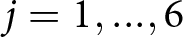$j=1, ..., 6 $, using the arithmetic mean, that we denote by 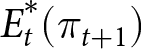$E^{*}_{t}(\pi_{t+1}) $ and 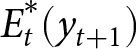$E^{*}_{t}(y_{t+1})$. These aggregate expectations are then inserted into the standard IS and Phillips curves given by:

(1)\begin{equation} \hat{y}_{t}=E^{*}_{t} \hat{y}_{t+1}-\sigma^{-1}\left(\hat{\imath}_{t}- E^{*}_{t} \hat{\pi}_{t+1}-\bar{r}\right)+ g_{t}, \end{equation}

(2)\begin{equation} \hat{\pi}_{t}=\beta E^{*}_{t} \hat{\pi}_{t+1}+\kappa\hat{y}_{t}+u_{t}, \end{equation}

where $\hat{y}_{t}$ is the output gap, $\hat{\pi}_{t}$ the inflation gap, that is the difference between inflation and the CB target $\pi^T$, $ g_{t}$ and $u_{t}$ exogenous real and cost-push shocks to be specified below, $\beta$ and $\sigma$ households’ preference parameters, $\kappa$ the slope of the Phillips curve and $\hat{\imath}_{t}$ the nominal interest rate set by the CB either with an IT or a PLT rule (depending on the experimental treatments, see Section 3.2), expressed in deviation from its steady-state level 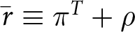$\bar{r} \equiv \pi^{T}+\rho$. We use the standard parameter values $\beta=0.994$, $\sigma=1$, $\kappa=0.0625$.

Each subsession starts with an initial learning phase for the subjects consisting of small white noise shocks around the targeted steady state. A severe, persistent and unannounced deflationary real shock then disturbs the economy in period 11 of Subsession 1 and a cost-push shock hits the economy in period 9 of Subsession 2.Footnote ⁹ The shock sequences are the same for all sessions and are displayed in Appendix B. In other words, we engineer two recessions in each experimental economy. In Subsession 1, the recession is coupled with low inflation and does not imply any stabilization trade-off but the severity of the initial shock induces an ELB episode in the model under RE independently of the monetary policy rule; see Section 3.2 and Fig. 1 below. By contrast, the recession in Subsession 2 is associated with inflationary pressures that imply a stabilization trade-off. Hence, we collect experimental data on the properties of IT and PLT in distinct economic environments. Additionally, to measure long-run inflation expectation anchoring in each environment, at period 26 of each subsession, we elicit a one-time inflation forecast for the end of the subsession that is, respectively, 15 and 10 periods later.

Fig 1.

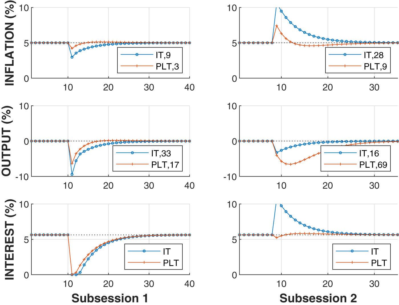
Simulations under RE

Fig 1 Long description

Inflation—Subsession 1: The graph shows inflation percentage over time, with the x-axis representing periods from 0 to 40 and the y-axis representing inflation percentage from 0 to 10. The IT series is marked with circles, showing a dip around period 10 and gradual recovery. The PLT series, marked with crosses, shows a smaller dip and steadier recovery. Inflation—Subsession 2: The graph shows a sharp spike in inflation for IT around period 10, followed by a decline. PLT shows a smaller spike and steadier decline. Output—Subsession 1: The graph shows output percentage over time, with the x-axis representing periods from 0 to 40 and the y-axis from negative 10 to 10. IT shows a sharp drop at period 10 and gradual recovery, while PLT shows a smaller drop and steadier recovery. Output—Subsession 2: IT shows a sharp drop followed by recovery, while PLT shows a smaller drop and slower recovery. Interest—Subsession 1: The graph shows interest percentage over time, with the x-axis representing periods from 0 to 40 and the y-axis from 0 to 10. IT shows a dip at period 10 and recovery, while PLT shows a smaller dip and steadier recovery. Interest—Subsession 2: IT shows a sharp spike at period 10, followed by a decline, while PLT shows a smaller spike and steadier decline. The graphs illustrate the differences in economic responses between IT and PLT across subsessions, highlighting the impact of shocks and recovery patterns.

Notes: The values in the boxes report the total absolute deviation (in p.p.) for IT (blue circles) and PLT (rec crosses). We use the occbin library in Dynare to account for the occasionally binding constraint (Guerrieri & Iacoviello, 2015). The shocks in the simulations are an AR(1) process with an autoregressive coefficient of 0.8 which fits the series of three negative shocks in the experiment.

The role of the subjects is framed as professional forecasters for a statistical bureau. The instructions – reproduced in Appendix F – explain the positive and negative relationships between the main variables in the economy and provide the value of the inflation target. All but a few pieces of information are identical across all treatments: the description of the monetary policy rule differs under IT and PLT, and subjects additionally receive an inflation guidance under the treatment that tests PLT with communication (see Section 3.2 below).Footnote ¹⁰ At the beginning of every period in all treatments, subjects observe the current and past shocks and all past endogenous variables, including the price level and its path consistent with the inflation target, which is labeled as ‘price level if inflation is always 5%’ under IT and ‘intended price level’ in the PLT treatments where the concept of price gap is also introduced in the instructions. All these pieces of information are displayed in a table and in charts on the graphical user interface (GUI), reproduced in Appendix F.2.

Importantly, and in contrast to the existing literature, subjects also observe the most recent forecasts of all other forecasters in their economy along with their payoff. An explicit ranking from the best to the worst forecasters in which each given subject is included (tagged by ‘YOU’) is updated in each period on a table on the GUI.Footnote ¹¹ In other words, subjects observe their peers’ forecasting performances and can assess their relative performances. This design aligns the information set of the subjects with that of the HENK agents in Section 5.2 and of real-world professional forecasters, and does not affect cross-treatment comparisons. Moreover, the slow convergence under IT and volatile oscillations under PLT at the ELB in Section 4 match prior findings discussed in Section 2, which speaks against peer imitation affecting forecasting incentives.

Finally, subjects accumulate points that reward their forecast accuracy throughout the experiment. In each period, a forecast brings $ \frac{100}{1+\text{absolute forecast errors in p.p.}}$ points, so that a perfect forecast brings 100 points. To rule out strategical hedging across the inflation and output forecasts, subjects accumulate a separate amount of forecasting points for each variable and only one of the two is randomly drawn at the end of the experiment to be converted into money at a rate of CA\$0.2 per 100 points. To reinforce the salience of the occasional long-run inflation forecasting task, the points corresponding to these two forecasts are converted at a rate of CA\$3 per 100 points.Footnote ¹²

3.2. Treatments and FIRE predictions

We implement three experimental treatments, denoted by IT, PLT, and PLT-G. Tr. IT differs from Trs. PLT and PLT-G only by the monetary rule that sets the nominal interest rate in Eq. (1). Under IT, the CB implements a standard contemporaneous Taylor rule subject to the ELB:

(3)\begin{equation} \mathbf{IT:} \; \hat{\imath}_{t}=\max \left\{0,\bar{r}+\phi^{\pi}\hat{\pi}_t+\phi_{IT}^{y}\hat{y}_t\right\}, \end{equation}

where the ELB is set to 0% and we use 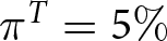$\pi^{T} = 5\%$ and $\phi^{\pi}_{IT} = 1.5, \phi^y=1$, which ensures determinacy under RE and stability under backward-looking expectations, see App. A.

In Trs. PLT and PLT-G, the CB uses a PLT monetary policy rule. It is convenient to define the price gap 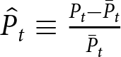$\hat{P}_t \equiv \frac{P_t-\bar{P}_t}{\bar{P}_t}$, which measures the gap between the current price level $P_t$ and its predetermined targeted level $\bar{P}_t$ that grows at a rate $\pi^T$ consistent with the CB inflation target. In the log-linearized model, the price gap evolves as $\hat{p}_{t}=\hat{p}_{t-1}+\hat{\pi}_{t}$. In Trs. PLT and PLT-G, the CB sets the interest rate using the following rule:

(4)\begin{equation} \mathbf{PLT:} \; \hat{\imath}_{t}=\max \left\{0,\bar{r}+\phi^{P} \hat{p}_{t}+\phi^{y}\hat{y}_t\right\}, \end{equation}

where we use 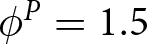$\phi^P=1.5$ so that the initial policy responses to the shocks are the same in all treatments (holding everything else equal) and determinacy under RE and stability under learning of the targeted steady state hold; see App. A.

Tr. PLT-G differs from Tr. PLT only by the provision to the subjects of an inflation guidance. In Tr. PLT-G, in each period, subjects receive an inflation guidance that corresponds to the implicit time-varying inflation level that would close the price gap in any period $t$. (see App. A for detail). Hence, the guidance, that we denote by $\pi_t^{CB}$, is model-consistent. Under the FIRE assumption, it is redundant because expectations are already model-consistent, and there is no difference between Trs PLT and PLT-G. Under real-world expectations however, the guidance may help subjects coordinate their expectations on the history-dependent path. In each period, subjects receive the guidance in a bold and highlighted manner on the GUI, and all previous guidance announcements are displayed on the inflation graph; see App. F.2.

The guidance carries the underlying structure of the PLT regime while keeping the frame of the CB communication in terms of inflation rather than price level, which we conjecture to be an easier-to-grasp and more practical communication regime for the public than a communication in terms of price levels.

More generally, we phrase monetary policy in terms of inflation rate under both IT and PLT, even though the price level may be the salient variable under PLT, and eliciting inflation expectations need not be equivalent to eliciting price-level expectations in terms of expectation formation and macroeconomic dynamics. Our choice is motivated by external validity concerns: in practice, policy institutions communicate in terms of inflation rates, not price levels. Significant resources are devoted to measuring and analyzing inflation expectations under the prevailing IT frameworks. Moreover, inflation, not the price level, underpins key economic measures such as real returns or wages, and international comparisons. In most macroeconomic models, nominal variables like the price level are also indeterminate, and the focus is thus placed on inflation dynamics. For these reasons, both academic and policy discussions of PLT are typically framed in terms of inflation rates, and so is our experiment.

Figure 1 provides the dynamics of the IT and PLT experimental economies under the FIRE benchmark given our calibration; see Appendix A for the derivations. In line with the discussion in introduction, it is clear that PLT is superior to IT for a CB primarily concerned with inflation stabilization. PLT better stabilizes inflation and output gaps than IT in the absence of policy trade-off (namely in face of deflationary pressures, see left panel), even though the ELB binds under both regimes (bottom left panel). When facing inflationary pressures (right panel), PLT better limits the rise in inflation but at the price of a deeper recession than under IT (middle right panel). Comparing inflation and output gap dynamics in the three treatments allow us to assess whether this ranking is robust to laboratory expectations.

3.3. Implementation

The experimental software was programmed using oTree (Chen et al., Reference Chen, Schonger and Wickens2016). A first batch of six experimental sessions for each of the three treatments was conducted in person at the CRABE lab at Simon Fraser University (SFU) between August and October 2022. Six additional sessions per treatment were added, two at SFU in January and February 2025 and four at the CREED lab of the University of Amsterdam in April of the same year, involving a total of 216 subjects. The robustness treatment PLT-G-R in Appendix D was also run with the same subject pool composition in 2025. The average duration of each session was just over two hours. In 2022, SFU participants earned an average of CA\$24.8 including a CA\$7 participation fee (from a minimum of 15 to a maximum of 38 with a standard deviation of 6.75), and CA\$31.16 with a standard deviation of 5.03 in 2025 following the post-COVID-19 SFU lab guidelines. Following the 2025 CREED guidelines, participants earned an average of € 36.9 (with a standard deviation of 7.3), which reflects higher payment expectations given a higher net minimum wage and higher recent inflation in the Netherlands than in Canada.

Upon entering the lab, subjects were provided with the instruction booklet which gives a qualitative overview of the relationships among the variables and clearly explain the tasks.Footnote ¹³ Subjects were then asked to carefully read the instructions and complete a comprehension quiz in order for the experiment to start. The forecasting game started with Subsession 1. All predictions were submitted on the GUI. At the end of the first subsession and before starting Subsession 2, subjects were provided with the updated instruction booklet that highlights the change in the shock, from real to cost-push shocks. We introduced information about the shocks in such a sequential manner to prime subjects towards the particular economic environment implemented while avoiding the cognitive overload that could result from simultaneous information about various types of shocks. Finally, at the end of the second subsession and before leaving the lab, the subjects were asked to complete an exit survey consisting of demographic questions, central banking literacy, and the strategy(ies) used in the experiment, if any.

4.1. Macroeconomic dynamics in the experimental economies

Figs 2-4 report the dynamics of inflation, output gap and interest rate in all experimental economies (dashed blue lines) in, respectively, Trs. IT, PLT, and PLT-G, along with the median realization over the 12 sessions in each treatment (red thick lines). In Tr. PLT-G, since we may not directly observe whether subjects use the CB guidance to form their inflation forecasts, we compute a “credibility index,” i.e. the distance between individual inflation forecasts and the guidance, averaged across all subjects for each period:

(5)\begin{equation} Cred_{t}^{CB}= \frac{1}{6}\sum_{j=1}^6 exp(-(\pi^{e}_{j,t+1}-\pi_t^{CB})^2), \end{equation}

where a higher value indicates a higher CB credibility. The bottom panel of Fig. 4 displays the dynamics of this credibility index in Tr. PLT-G.

Fig 2.

Inflation, output gap and interest rate dynamics in Tr. IT

Fig 2 Long description

The figure consists of six line plots illustrating the dynamics of inflation, output and interest rates over time in two subsessions. Each plot has a y-axis labeled in percent and an x-axis representing time in periods. The top row shows inflation, the middle row shows output and the bottom row shows interest rates. The left column represents Subsession 1 and the right column represents Subsession 2. In each plot, dashed blue lines represent individual experimental sessions, while a solid red line indicates the median realization. A vertical dashed line marks the time of a large shock, occurring around period 10. In Subsession 1, inflation initially decreases sharply after the shock, reaching a trough around period 20, then gradually returns toward zero. Output shows a similar pattern, with a significant drop post-shock and recovery by period 40. Interest rates rise sharply after the shock, peaking around period 20, before stabilizing. In Subsession 2, inflation rises after the shock, peaking around period 15, then declines toward zero. Output decreases post-shock, with a gradual return to baseline. Interest rates increase sharply, peaking around period 15, then stabilize. The plots highlight the response dynamics to the shock across different economic variables.

Fig 3.

Inflation, output gap and interest rate dynamics in Tr. PLT

Fig 3 Long description

The multi-line graphs illustrate inflation, output and interest rate dynamics across two subsessions. The x-axis represents time periods, while the y-axis measures percentage deviations from baseline, ranging from negative 10 to positive 10 percent. Each graph includes lines for experimental sessions and median values, with vertical dashed lines marking the time of large shocks. In Subsession 1, inflation shows fluctuations with peaks around time 15 and 30, output peaks near time 20 and interest rates peak around time 25. Subsession 2 displays similar patterns, with inflation peaking near time 10 and 25, output peaking around time 15 and interest rates peaking near time 20. The experimental session lines are dashed, while median values are solid. The graphs demonstrate how inflation, output and interest rates respond to large shocks, with median values smoothing volatility. Subsession 2 shows slightly different dynamics compared to Subsession 1, indicating varied responses to shocks. The purpose is to analyze the impact of large shocks on economic variables and the stabilizing effect of median values.

Fig 4.

Inflation, output gap and interest rate dynamics in Tr. PLT-G

Fig 4 Long description

The figure consists of eight line plots displaying inflation, output, interest and credibility index over time across two subsessions. Each plot has the x-axis labeled as ′Subsession′ with periods ranging from 0 to 40 for Subsession 1 and 0 to 35 for Subsession 2. The y-axes are labeled as follows: inflation in percent, output in percent, interest in percent and credibility index ranging from 0 to 1. Dashed blue lines represent individual experimental sessions, while red thick lines indicate the median realization. A vertical dashed line marks the ′Time of Large Shock.′ In Subsession 1, inflation, output and interest show a sharp dip around the shock, followed by a gradual return to baseline. The credibility index fluctuates significantly. In Subsession 2, similar patterns are observed with variations in timing and magnitude. The plots illustrate the dynamic responses to economic shocks, with notable peaks and troughs in each variable.

Table 1 reports cross-treatment comparisons regarding inflation and output gap stabilization. To do so, we compute the per-period average of the absolute deviation (AAD) of inflation and output gap from their targets. For each session $s=1, .., 12$ and subsession 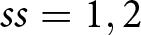$ss=1, 2$ with a given duration of 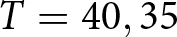$T=40,35$ periods, the AAD for each variable reads as:

(6)\begin{equation} AAD_{s,ss}^\pi=\frac{1}{T}\sum_{t \in T}|\pi_{s,ss,t}-\pi^T| \text{ and } AAD_{s,ss}^y=\frac{1}{T}\sum_{t \in T}|y_{s,ss,t}|, \end{equation}

where lower values indicate a better stabilization of inflation and output gap. In Table 1, we disentangle pre-shock (top panel) from post-shock periods, which include the shock periods themselves (bottom panel).

Table 1.

Cross-treatment comparisons of inflation and output gap in the experiment

Table 1 Long description

Cross-treatment results report average absolute deviations from target for inflation and the output gap, split into pre-shock and post-shock panels and two subgroups, with standard deviations in parentheses and pairwise p-values. Pre-shock inflation deviations are similar for IT and PLT in subgroup 1 (about 0.68 and 0.67) but lower under PLT-G (0.32), with significant differences versus PLT-G (p 0.03 for both comparisons). Pre-shock inflation in subgroup 2 is much higher under PLT (2.07) than IT (0.67) or PLT-G (0.28), and PLT differs from PLT-G at less than 0.01. Pre-shock output-gap deviations are far larger under PLT (2.65 and 4.55) than IT (0.47 and 0.32) and PLT-G (1.51 and 0.87), with IT versus PLT significant at less than 0.01 in both subgroups. Post-shock, PLT deviations rise sharply for both inflation (5.14 and 10.33) and the output gap (11.10 and 19.99), while IT and PLT-G remain much lower (inflation roughly 0.36 to 1.56; output gap roughly 0.76 to 3.5). Many post-shock comparisons involving PLT are significant at less than 0.01, and IT versus PLT-G is sometimes not significant (for example, subgroup 2 inflation p 0.38 and subgroup 1 output gap p 0.38). P-values come from nonparametric rank-sum tests at the matching-group level and are adjusted for multiple comparisons, so significance reflects those corrections.

Note: The average of the absolute deviation (AAD) of inflation π and output y from their target displayed in the first three columns are computed as per Eq. (6) and are averaged across all 12 sessions of each treatment. Standard deviations are reported between brackets. The p-values displayed in the last three columns correspond to the non-parametric Wilcoxon rank-sum tests for comparison between each pair of treatments performed at the matching group level with N = 12 observations per treatment. The p-values are adjusted for multiple comparisons with the Holm (Reference Holm1979) sequentially-rejective procedure.

Overall, the merits of PLT under FIRE do not extend to the lab environment: experimental economies under PLT are more unstable than under IT. However, once augmented with CB guidance in Tr. PLT-G, the stabilization benefits of PLT materialize in the lab and this treatment delivers the smallest inflation gap.

In detail, in the first periods of each subsession – i.e. before the shocks, inflation and output appear similarly stabilized around their target under IT and PLT with guidance while displaying wilder oscillations under PLT. This visual impression is confirmed by the cross-treatment comparisons of the AADs (top panel of Table 1). The ADDs of inflation and output are significantly higher in Tr. PLT than in Trs. IT and PLT-G. In the aftermath of the large shocks, in both subsessions, the cross-treatment differences become even more salient: while economies in IT and PLT-G eventually converge back to the targeted steady-state, economies in Tr. PLT exhibit wilder and non-dampening oscillations. The bottom panel of Table 1 reports that the AADs of both inflation and output gap are considerably and significantly higher in Tr. PLT than in Trs. IT and PLT-G. The standard deviations of the AADs under PLT are also strikingly larger than in the two other treatments, which indicates more variation across independent economies.

Even if inflation returns towards the target in both Trs. IT and PLT-G, the inflation gap under IT exhibits more persistence in the aftermath of the recessions. Inflation remains persistently below target in the deflationary shock subsession (left panel) and persistently above target in the cost-push shock subsession (right panel). These observations are consistent with the persistently low inflation experience post-Great Financial Crisis and the persistently high inflation in the post-COVID-19 pandemic. These circumstances result in an unanchoring of inflation expectations, see Section 4.2, consistent with the hoovering of the one-year-ahead inflation forecasts from professionals (SPF) below 2% in the US and the Euro area over the 2010 decade, and the recent landing of both household and professional one-year-ahead inflation forecasts toward 3% in the US (see the SPF and Michigan household survey as of 2024Q4).

By contrast, in Tr. PLT-G, inflation returns to the target in a quicker time frame than under IT with negligible fluctuations, as shown in Fig. 4. This inflation stabilization in Tr. PLT-G is observed under both types of shocks but is most salient after the deflationary shock. In particular, in the wake of the deflationary recession, the ELB binds for a median time of only two periods under Tr. PLT-G, in line with the FIRE benchmark and considerably less than the four periods of ELB in Tr. IT. Looking at the credibility index in Tr. PLT-G (bottom panel of Fig. 4), while credibility substantially drops at the onset of the recessions, it increases back toward one (full credibility) along the recoveries. Finally, in line with the FIRE prediction, a better inflation stabilization in Tr. PLT-G than in Tr. IT comes at the cost of a wider output gap, in particular after a cost-push shock. This is confirmed in the bottom panel of Table 1: the output gap in Subsession 2 is significantly wider in Tr. PLT-G than under Tr. IT.

We now turn to the analysis of individual forecasts.

4.2. Heterogeneity in individual forecasts

Fig. 5 reports the median short-run forecast dispersion across all 12 sessions of each treatment, measured by the standard deviation of the distribution of forecasts of the six subjects in each period. Table 2 complements the graphical analysis with the corresponding cross-treatment comparative statistics.

Fig 5.

Between-subject disagreement in short-run forecasts

Fig 5 Long description

The figure consists of four line graphs arranged in a two-by-two grid. The top row shows inflation trends and the bottom row shows output trends. Each column represents a different subsession, labeled as Subsession 1 and Subsession 2. The x-axis for all graphs is labeled ′Subsession′ with a range from 0 to 40. The y-axis for the top graphs is labeled ′Inflation′ with a range from 0 to 6 and for the bottom graphs, it is labeled ′Output′ with a range from 0 to 8. Each graph includes three lines representing different treatments: IT (solid blue line), PLT (dotted orange line) and PLT-G (dashed red line). A vertical dashed black line indicates the ′Time of Large Shock′ at approximately the 10 mark on the x-axis. In Subsession 1, the PLT line shows a sharp peak in inflation and output shortly after the shock, while IT and PLT-G remain relatively stable. In Subsession 2, similar patterns are observed, with PLT showing more volatility compared to IT and PLT-G.

Note: Median over time (x-axis) across all 12 sessions in each treatment in p.p. (y-axis).

Table 2.

Cross-treatment comparisons of subjects’ forecasts in the experiment

Table 2 Long description

Cross-treatment results report average disagreement in short-run forecasts (inflation and output) before and after a shock, plus long-run inflation forecasts, shown separately for Subsession 1 and Subsession 2. In the pre-shock short-run panel, PLT generally has higher disagreement than IT and PLT-G: for example, output disagreement in Subsession 1 is 1.91 under PLT versus 0.80 under IT, with a p-value of 0.04 for IT versus PLT. In Subsession 2 pre-shock, PLT is much higher than both IT and PLT-G for inflation (1.19 versus 0.35 and 0.32) and for output (1.87 versus 0.20 and 0.44), with p-values below 0.01 for PLT compared with each alternative. In the post-shock short-run panel, PLT remains the highest across all rows, such as output disagreement in Subsession 2 at 3.15 under PLT versus 0.43 under IT and 1.31 under PLT-G, with all pairwise p-values below 0.01. Differences between IT and PLT-G are often smaller and sometimes not statistically significant, such as post-shock inflation disagreement in Subsession 1 (0.43 versus 0.33; p-value 0.48). Long-run inflation forecasts are similar across treatments in Subsession 2 (around 5.40 for IT and PLT-G, 1.39 for PLT) with p-values reported as greater than 0.99 for all pairwise comparisons, indicating no detected differences there. In Subsession 1 long-run inflation, PLT-G is higher (5.39) than IT (4.37) with a p-value of 0.03, while IT versus PLT is not statistically significant (p-value 0.12). Values in parentheses are dispersion measures, and p-values reflect pairwise comparisons rather than effect sizes.

Note: See Table 1. Forecast disagreement (top and middle panel) is computed as the standard deviation across the six forecasts in each period and is averaged over the 12 sessions of each treatment. The bottom panel reports the average of the long-run inflation forecasts, elicited once per subsession for the final period of the subsession. The associated p-values report pairwise cross-treatment comparisons.

Forecast dispersion varies both within treatments, i.e. over time, and between treatments. From Fig. 5, we see that pre-shock forecast dispersion declines in all treatments and subsessions, especially in Trs. IT and PLT-G, which suggests that subjects learn to coordinate on the target in the absence of large shocks in these two treatments. Table 2 (top panel) indicates that pre-shock disagreement is similar across treatments in Subsession 1 but significantly higher in Subsession 2 under Tr. PLT than in the two other treatments.

In the wake of the shocks, forecast dispersion rises in all treatments. In Trs. IT and PLT-G, in line with the better stabilization of the endogenous variables compared to Tr. PLT, forecast dispersion tends to revert back towards its pre-shock level, while it remains persistently elevated in Tr. PLT.Footnote ¹⁴ The statistical tests reported in the middle panel of Table 2 confirm this pattern: after the shocks, short-run forecasts are significantly more dispersed under Tr. PLT than under Trs. IT and PLT-G. By contrast, forecast dispersion is not significantly different between Trs. IT and PLT-G, except for output forecasts after the cost-push shock in Subsession 2 which are more dispersed under PLT-G than under IT. This difference is consistent with the sharper stabilization trade-off and resulting steeper output drop in the wake of the shock under PLT than under IT discussed above. However, Fig. 5 shows that, by the end of Subsession 2, output forecast dispersion converges to a negligible level in Tr. PLT-G, comparable to the level observed in Tr. IT, while it remains elevated in Tr. PLT.

The bottom panel of Table 2 reports the average long-run inflation forecasts (namely for the final period of each subsession) across all subjects, which speaks to cross-treatment differences in the level of long-run expectations in each subsession. Fig. A.2 plots their distributions, which illustrates their dispersion. While we cannot find any statistically significant difference across the three treatments in their level, their distribution differs sharply: under Tr. PLT, long-run forecasts are strikingly more dispersed, especially in Subsession 2, whereas they remain more tightly concentrated around the target under Trs. IT and PLT-G.

To gain further insights into long-run anchoring of expectations, Table 3 reports the estimated asymptotic values of the short-run forecasts, in deviation from the target, using the method of Duffy (Reference Duffy, Kagel and Roth2016). Short-run forecasts converge to the target in a strong sense only in Tr. PLT-G, with the asymptote being the largest in Tr. PLT.Footnote ¹⁵

Table 3.

Asymptote estimates of the deviation of the average short-run inflation forecasts from the target

Table 3 Long description

Asymptote estimates summarize the long-run deviation of average short-run inflation forecasts from the target under three regimes: IT, PLT, and PLT-G. IT has an estimate of minus 0.15 with a standard deviation of 1.39, and p-values 0.40 and 0.32, indicating weak evidence that forecasts converge within the stated tolerance band. PLT shows a much larger negative estimate, minus 5.79, with a very large standard deviation of 11.36 and p-values 0.68 and 0.29, also suggesting little evidence of convergence. PLT-G is essentially zero, minus 0.003, with a standard deviation of 0.33 and p-values 0.06 and 0.06, marked with a single star to indicate rejection of non-convergence at the 10 percent level. Overall, PLT-G appears most consistent with long-run forecasts aligning with the target, while IT and especially PLT are more negative and less precise. Results rely on an autoregressive model and an equivalence-style test, so p-values reflect evidence for being within a tolerance band rather than a standard difference-from-zero test.

Note: Estimated mean of an AR(1) process on short-run inflation forecasts, averaged per period at the treatment level; see Duffy (Reference Duffy, Kagel and Roth2016). The p-values refer to the equivalence test using the two one-sided test (TOST) procedure where the null hypothesis is a deviation of the asymptotic forecast value from a 10%-radius of the 5% target, and the alternative hypothesis is the convergence of the long-run forecasts within 10% of the target. ***, ** and * indicate that non-convergence is rejected at 1, 5, and 10%.

To conclude, we highlight the two main experimental results:

We now dig further into individual forecast data.

4.3. Expectation formation and evidence of peer imitation

We first use panel models at the subject-period level to identify which pieces of the available information significantly relate to the inflation and output forecasts in each treatment. The details of the models are deferred to Table A.1 in App. C. The main takeaway is that the subjects react to the most recent inflation and output gap values, their own latest forecasts, the best forecasts in their group and, to a lesser extent, the shocks. They never react to the past price gap, which indicates that expectations are not model-consistent in Tr. PLT. Moreover, consistent with prior experimental findings (e.g., Assenza et al., Reference Assenza, Heemeijer, Hommes and Massaro2021), inflation and output gap forecasts appear decoupled: inflation forecasts respond primarily to past inflation and past inflation forecasts, while output gap forecasts are linked to their own respective histories, with minimal cross-influence.

To refine our description of the forecasts and uncover evidence of peer imitation, we estimate heuristics on the forecast time series for each subject. We modify the set of heuristics that usually approximate well the forecasting behaviors of the subjects in this class of experimentsFootnote ¹⁶ to include the forecasts of the most accurate forecaster of the group in any given period. We denote this additional piece of information by $\pi^e_{BF,t}$. For each subject, we estimate the following inflation forecasting models:

(7)\begin{equation} \pi^e_{t+1} = f(\pi^e_{BF,t}) + \epsilon_t, \end{equation}

(8)\begin{equation} \pi^e_{t+1} = f(\pi^e_{BF,t},\pi^e_{t}) + \epsilon_t, \end{equation}

(9)\begin{equation} \pi^e_{t+1} = f(\pi_{t-1},\pi_{t-2}) + \epsilon_t, \end{equation}

(10)\begin{equation} \pi^e_{t+1} = f(\pi_{t-1},\pi_{t-2},\pi^e_{BF,t}) + \epsilon_t, \end{equation}

(11)\begin{equation} \pi^e_{t+1} = f(\pi_{t-1},\pi_{t-2},\pi^e_{BF,t},\pi^e_{t},F_t) + \epsilon_t, \end{equation}

(12)\begin{equation} \pi^e_{t+1} = f(\pi^e_{t},\pi_{t-1}) + \epsilon_t, \end{equation}

(13)\begin{equation} \pi^e_{t+1} = f(F_t) + \epsilon_t, \end{equation}

(14)\begin{equation} \pi^e_{t+1} = f(\pi_{t-1},\pi_{t-2},F_t) + \epsilon_t, \end{equation}

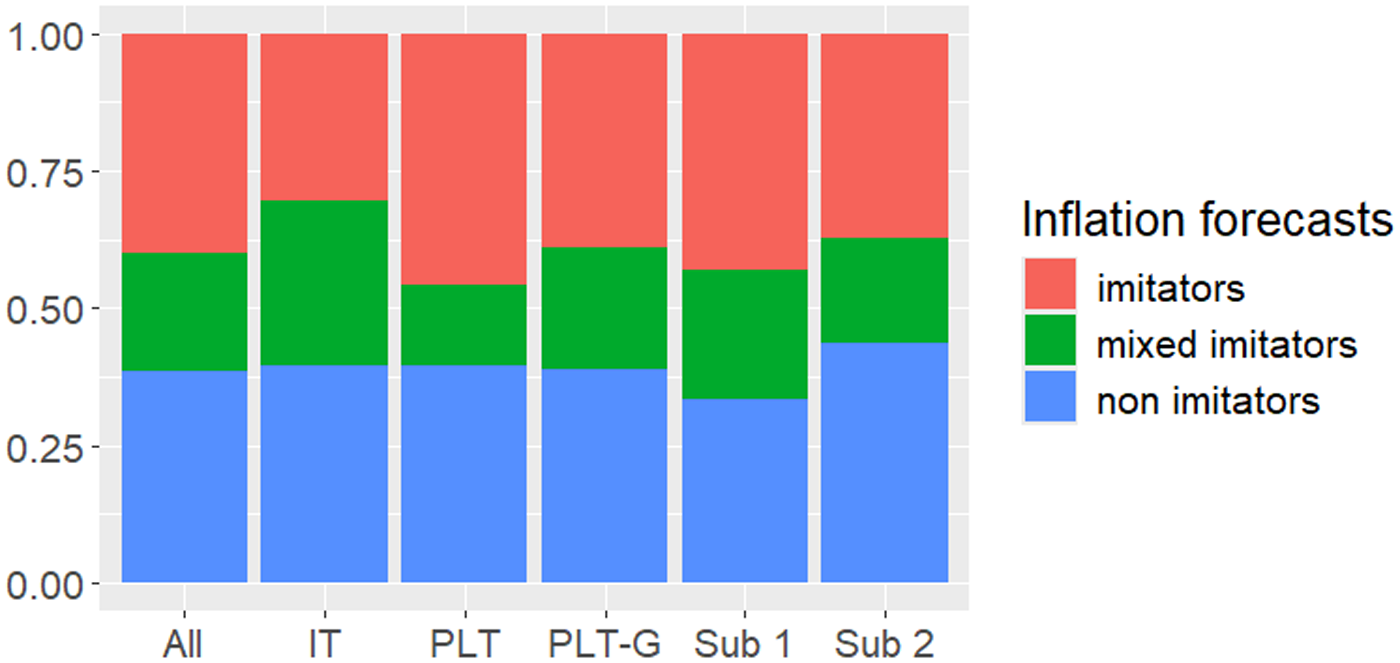
where $f(\cdot)$ is a linear function in its arguments. Models (7), (8), (10) and (11) make use of the best forecasts and correspond to “imitation models.” Model (7) is a “copy-cat” strategy that consists in adopting the best forecast. Model (8) also relies on the individual previous forecasts and may therefore be defined as an “adaptive imitator.” Model (10) corresponds to an “anchoring-and-adjustment” rule where the anchor is the best forecast and the adjustments take place in the direction of the most recent inflation trend. Model (11) is a mixed model where all these pieces of information are used to make predictions. Models (9), (12) (13) and (14) are the four benchmarks discussed in Footnote 16. We include these standard ‘non-imitation’ models to allow for the possibility that subjects do not significantly imitate. We use the Akaike Information Criterion (AIC) to classify each subject across one of these forecasting heuristics. The results are presented in Fig. 6 for inflation forecasts and in Fig. A.4 for output gap forecasts, where we show the fraction of ‘imitators’ (defined as subjects assigned to Models (7), (8) or (10)), ‘mixed imitators’ (assigned to Model (11)) and non-imitators (assigned to any other models) over all sessions, per treatment and subsession.

Fig 6.

Proportions of imitation, mixed and non-imitation heuristics among all subjects

Overall, we find evidence of peer imitation, and to a similar extent in both inflation and output gap forecasts and across treatments.Footnote ¹⁷ Imitation may arise due to the complexity of the environment or strategic complementarities in the NK models, where aligning with others’ expectations is payoff-enhancing. Salient reference points – like the best forecaster’s predictions or the CB guidance – can serve as coordination devices since they are self-fulfilling.

Finally, Fig. A.3 plots the distributions of the estimated coefficients of the imitation models. The coefficient values are consistent with the interpretation of each rule. In the “copycat” model (7), the estimated coefficients associated with the best forecasts are distributed around 1 (see the top-left panel of Fig. A.3). In the “anchoring-and-adjustment” rule (10), the coefficients associated with the past two inflation lags are of the same magnitude on the unit interval but of opposite signs, which is consistent with an adjustment in line with the latest inflation trend (see top-right panel). The “adaptive imitator” model (8) reflects a weighted average between the best forecast and the latest inflation (see bottom-left panel). The estimated coefficients associated with these pieces of information remain of the same order of magnitude in the mixed model (see bottom-right panel).

We now use a behavioral model with peer imitation to rationalize the lab data.

5.1. Overview of the HENK model

We describe here expectations in the HENK model, based on a simplified version of Arifovic et al. (Reference Arifovic, Grimaud, Salle and Vermandel2025), and refer to Appendix E for detail. Each agent $j$ enters each period with their own inflation and output gap forecasts $\xi^{x}_{j,t-1} $, 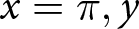$x=\pi, y$. They then receive private news $\iota^{x}_{j,t}$ which modifies their forecasts into: $m^x_{j,t} \equiv \xi^x_{j,t-1} + \iota^{x}_{j,t}$, $x=\{y, \pi\}$. Each updated belief $m$ is evaluated using its ‘Foregone’ error, denoted by $F_{j,t}^{x} \equiv (\hat{x}_{t-1}-m_{j,t}^{x})^{2}$, which represents the forecast error that the agent would have made in $t-1$ had they used $m^x$ as a forecast for $x$. Finally, agents are paired for peer imitation, and the one with the higher foregone error adopts the other’s beliefs, which sets $\xi^{x}_{j,t}$. This process repeats itself in the next period.

With CB guidance, agents have a third element, a “credibility” level, denoted by $c_{j,t} \in [0,1]$, that is their probability of aligning their inflation forecast with the guidance, instead of using their own belief. This component is also modified by news. The foregone inflation forecast error is adjusted to reflect the weighted average of the two errors under the two forecasting strategies, i.e. $F_{j, t}^{\pi}=c_{j, t}\left(\hat{\pi}_{t-1}-\pi_{t}^{C B}\right)^{2} +\left(1-c_{j, t}\right)\left(\hat{\pi}_{t-1}-m_{j, t}^{\pi}\right)^{2}$. The CB guidance does not affect output gap expectations.

Expectations are initialized around the steady state so that the news are the only processes to be specified, which ensures parsimony. We use independent Gaussian draws $\iota^x_{j,t}\sim \mathcal{N}(\theta^x(g_{t}, u_{t}), \sigma_x)$, $x=y, \pi, c$, where the ‘average news’ $\theta^x$ about variable $x$ linearly depends on the latest observable shocks so that the news convey some fundamental information while keeping an unconditional zero mean. Since the instructions qualitatively describe the effects of the shocks, we impose 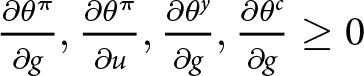$\frac{\partial \theta^{\pi}}{\partial g}, \frac{\partial \theta^{\pi}}{\partial u}, \frac{\partial \theta^{y}}{\partial g}, \frac{\partial \theta^{c}}{\partial g}\geq 0$ and $\frac{\partial \theta^{y}}{\partial u}, \frac{\partial \theta^{c}}{\partial u} \leq 0$, which means that in the model, the negative real shock $g$ in Subsession 1 tends to decrease inflation expectations, credibility and output gap outlooks, and a positive cost-push shock in Subsession 2 tends to bring inflationary and recessionary prospects with a lower CB credibility.

The model is simulated without any input from the experiment besides the time series of the shocks and the parameter values of the New Keynesian model. The information set of the HENK agents is consistent with that of the experimental subjects and the model nests the RE benchmark, which avoids taking an ex-ante stand on the nature of expectations that generates the experimental dynamics.

5.2. Cross-treatment comparisons

Figs 7-9 plot the simulated counterparts of Figs 2-4 under, respectively, IT, PLT and PLT-G, along with the median realizations in the experiment. A first glance at the figures reveals that the model can account for the main five stylized facts of the experiment.

First, inflation and output exhibit wilder and non-dampening oscillations under PLT compared to the stabilization observed towards the end of the subsessions under IT and PLT-G. Second, inflation returns to the target more quickly under PLT-G, along mild, symmetric oscillations, than under IT, where the inflation gap is more persistent – negative in the first subsession and positive in the second. Third, this persistence translates into a fairly long episode of low nominal interest rates in Subsession 1 under IT, which echoes the ‘low-for-long’ narrative up until 2021. It is different under PLT-G, where the nominal rate converges back to steady state after a few periods only. Fourth, even under PLT-G, the macroeconomic oscillations contrast with the RE dynamics. Fifth, the recession after the cost-push shock in Subsession 2 under PLT-G is larger than under IT.

Fig 7.

Inflation, output gap and interest rate dynamics under IT in the HENK model

Fig 7 Long description

Three multi-line graphs with a legend reading 90 percent Interval, Median, Median experimental counterpart. The horizontal axis on all three graphs shows values from 0 to 40. The vertical axis labels are INFLATION (percent), OUTPUT (percent) and INTEREST (percent). Each graph contains a 90 percent Interval band and two median lines labeled Median and Median experimental counterpart. INFLATION (percent) graph, x-axis range 0 to 40, y-axis label INFLATION (percent). Tick labels visible include 0 on the y-axis. The Median line drops below 0 after the start, reaches a low point around the middle of the horizontal range, then rises toward 0 by the end. The Median experimental counterpart follows a similar shape with smaller deviations. OUTPUT (percent) graph, x-axis range 0 to 40, y-axis label OUTPUT (percent). Tick labels visible include 0 on the y-axis. The Median line dips below 0 early, reaches a trough around the first third of the horizontal range, then returns toward 0 and stays near 0 through the end. The Median experimental counterpart follows a similar dip and recovery. INTEREST (percent) graph, x-axis range 0 to 40, y-axis label INTEREST (percent). Tick labels visible include 0 on the y-axis. The Median line falls sharply below 0 early, reaches the lowest point shortly after the start, then rises steadily toward 0 and remains slightly below 0 near the end. The Median experimental counterpart follows the same sharp drop and recovery pattern. Text below these three graphs reads Subsession 1. Three multi-line graphs with the same legend items: 90 percent Interval, Median, Median experimental counterpart. The horizontal axis on all three graphs shows values from 0 to 35. The vertical axis tick labels visible include 0 and 10 on the first graph, negative 10, 0 and 10 on the second graph and 0 and 10 on the third graph. Each graph contains a 90 percent Interval band and two median lines labeled Median and Median experimental counterpart. First graph, x-axis range 0 to 35, y-axis tick labels 0 and 10. The Median line rises from near 0 to a higher level around the first third of the horizontal range, then gradually declines and levels off above 0. The Median experimental counterpart follows a similar rise and leveling pattern. Second graph, x-axis range 0 to 35, y-axis tick labels negative 10, 0, 10. The Median line drops below 0 early, then returns toward 0 and stays close to 0 for the remainder. The Median experimental counterpart follows a similar drop and return. Third graph, x-axis range 0 to 35, y-axis tick labels 0 and 10. The Median line increases from near 0 to a higher level around the first third of the horizontal range, then slowly declines and levels off above 0. The Median experimental counterpart follows a similar increase and leveling pattern. Text below these three graphs reads Subsession 2.

Notes: 100 Monte Carlo simulations of the HENK model, see Appendix E for detail.

Fig 8.

Inflation, output gap and interest rate dynamics under PLT in the HENK model

Fig 8 Long description

Six time-series plots arranged in three rows and two columns, with row labels INFLATION (percent), OUTPUT (percent) and INTEREST (percent). The bottom labels read Subsession 1 for the left column and Subsession 2 for the right column. A legend at the top lists 90 percent Interval, Median and Median experimental counterpart. Top-left plot (Inflation). The x-axis has tick labels 0, 10, 20, 30, 40. The y-axis label is INFLATION (percent). Three lines and a dashed interval band are shown. The median line stays near 0 from 0 to about 15, rises to about 2 to 3 around 20, then declines toward about 1 by 40. The experimental counterpart line rises above the median around 15 to 25, reaching about 4 to 5 near 25 to 30, then falls toward about 2 by 40. The 90 percent interval widens after about 15, with the upper dashed line reaching around 6 to 7 near 30 to 35 and the lower dashed line near about minus 1 to 0. Top-right plot (Inflation). The x-axis has tick labels 0, 5, 10, 15, 20, 25, 30, 35. The y-axis label is INFLATION (percent). The median line is near 0 to 1 up to about 10, rises to around 3 near 15, then declines toward about 0 by 35. The experimental counterpart line drops below 0 around 10 to 20, reaching about minus 3 to minus 4 near 15 to 20, then rises back toward about 0 to 1 by 35. The 90 percent interval expands after about 10, with the upper dashed line around 5 to 6 near 15 to 20 and the lower dashed line around minus 5 to minus 6 near 15 to 20. Middle-left plot (Output). The x-axis has tick labels 0, 10, 20, 30, 40. The y-axis label is OUTPUT (percent). The median line starts near 0, declines to about minus 2 to minus 3 by about 10, rises to around 2 to 3 near 20, then declines to around minus 2 to minus 3 by 40. The experimental counterpart line falls to around minus 4 to minus 5 near 10 to 15, rises to around 3 to 4 near 20 to 25, then falls again toward about minus 4 by 40. The 90 percent interval is narrow early and wider after about 10, with upper values around 5 to 6 near 20 to 30 and lower values around minus 6 to minus 7 near 30 to 40. Middle-right plot (Output). The x-axis has tick labels 0, 5, 10, 15, 20, 25, 30, 35. The y-axis label is OUTPUT (percent), with visible tick labels including 10, 0 and minus 10. The median line declines from near 0 to about minus 6 to minus 8 by about 15, then rises toward about minus 2 to 0 by about 30 to 35. The experimental counterpart line drops more sharply to around minus 10 near 15 to 20, then rises toward about minus 2 to 0 by about 30 to 35. The experimental counterpart also shows a rise above 0 around 25 to 30, reaching about 2 to 3, then returning toward 0 by 35. The 90 percent interval widens after about 10, with the upper dashed line reaching around 6 to 8 near 25 to 35 and the lower dashed line reaching around minus 12 to minus 14 near 15 to 20. Bottom-left plot (Interest). The x-axis has tick labels 0, 10, 20, 30, 40. The y-axis label is INTEREST (percent). The median line starts near 0, drops to around minus 8 to minus 10 near 10, then rises to around 4 to 6 near 25 to 30 and ends near about 2 to 3 by 40. The experimental counterpart line drops below the median around 5 to 15, then rises to around 6 to 8 near 25 to 30 and declines toward about 3 to 4 by 40. The 90 percent interval is widest around 10 to 25, with the lower dashed line near about minus 12 to minus 14 and the upper dashed line near about 10 to 12. Bottom-right plot (Interest). The x-axis has tick labels 0, 5, 10, 15, 20, 25, 30, 35. The y-axis label is INTEREST (percent), with visible tick labels including 5, 0 and minus 5. The median line declines from near 0 to around minus 6 to minus 8 by about 15 to 20, then rises toward about minus 2 to 0 by about 30 to 35. The experimental counterpart line rises above 0 around 20 to 25, reaching about 4 to 6, then drops toward about 0 to minus 2 by 35. The 90 percent interval widens after about 10, with the upper dashed line reaching around 6 to 8 near 25 to 35 and the lower dashed line reaching around minus 10 to minus 12 near 15 to 20.

Notes: see Fig. 7

Fig 9.

Inflation, output gap and interest rate under PLT-G in the HENK model

Fig 9 Long description

Eight multi-line graphs are arranged in two columns and four rows. The left column is labeled Subsession 1 and the right column is labeled Subsession 2. Each graph contains three series: a dashed line representing the 90 percent interval, a solid line representing the median and a solid line representing the median experimental counterpart. The four row labels on the vertical axis are Inflation (percent), Output (percent), Interest (percent) and Credibility (percent). Subsession 1 x-axis runs from 0 to 40 in increments of 10. Subsession 2 x-axis runs from 0 to 35 in increments of 5. Inflation (percent), Subsession 1: The y-axis ranges from approximately negative 5 to positive 5. The median and median experimental counterpart lines begin near 0, rise to a peak of approximately 5 near session 15, then decline back toward 0 by session 20 and remain near 0 through session 40. The 90 percent interval dashed lines widen around sessions 10 to 20 and narrow thereafter. Inflation (percent), Subsession 2: The y-axis ranges from approximately negative 5 to positive 5. A prominent spike occurs near session 5 reaching approximately 5, followed by a dip to approximately negative 2 near session 10. The median experimental counterpart line overshoots the median near the peak around session 5. Output (percent), Subsession 1: The y-axis ranges from approximately negative 5 to positive 5. The lines dip to a trough near negative 5 around session 10, recover toward 0 by session 20 and remain near 0 through session 40. The median experimental counterpart follows the median closely but shows a slightly deeper trough. Output (percent), Subsession 2: The y-axis ranges from approximately negative 5 to positive 5. A trough of approximately negative 5 occurs near session 10, with recovery toward 0 by session 20. The median experimental counterpart dips more sharply than the median near session 10. Interest (percent), Subsession 1: The y-axis ranges from approximately negative 5 to positive 10. The lines peak near 10 around session 10, decline toward 0 by session 20 and stabilize near 0 through session 40. The dashed 90 percent interval is widest near session 10. Interest (percent), Subsession 2: The y-axis ranges from approximately negative 5 to positive 10. A peak near 10 occurs around session 5, followed by a decline to near 0 by session 15. The median experimental counterpart rises more steeply and recovers faster than the median. Credibility (percent), Subsession 1: The y-axis ranges from 0 to 100. The lines begin near 100, drop sharply to approximately 50 near session 10, then gradually recover toward 100 by session 40. The median experimental counterpart drops slightly further than the median near session 10. Credibility (percent), Subsession 2: The y-axis ranges from 0 to 100. A sharp decline to approximately 50 occurs near session 10, followed by a recovery toward 100 by session 30. The median experimental counterpart shows a deeper initial drop compared to the median.

Notes: see Fig. 7. The aggregate credibility ̄ct of the CB (last row) is defined as the average of the individual components cj,t across the agents in each period.

These cross-treatment differences are confirmed by statistical tests in Table 4. At least qualitatively, Table 4 replicates its counterpart Table 1. Before the shocks (top panel), IT and PLT-G regimes exhibit similar AAD-levels but the picture changes after the shocks (middle panel). PLT-G has the lowest inflation AAD and IT has the lowest output AAD, implying a quicker closure of the inflation gap under PLT-G, but at a higher stabilization cost in terms of output than under IT. Without guidance, PLT exhibits the largest AADs. Inflation differences are less pronounced than for output because the large oscillations under PLT emerge later in the simulations than in the experiment. Extrapolating the model for a few more periods reveals increasing volatility, consistent with the experiment (see Fig. A.5).

Table 4.

Cross-treatment comparisons in the simulations

Table 4 Long description

Cross-treatment simulation results report average absolute disagreement in percentage points for inflation and output, split into two subsamples, with pairwise p-values for IT versus PLT, IT versus PLT-G, and PLT versus PLT-G. In pre-shock inflation disagreement, PLT-G is lowest (0.13 and 0.10) versus IT (0.36 and 0.37) and PLT (0.27 and 0.31), with p-values below 0.01 for comparisons involving PLT-G and a smaller IT versus PLT difference (p-value 0.01 and 0.13). In pre-shock output disagreement, PLT is highest (1.55 and 1.12) while IT and PLT-G are lower (IT 0.70 and 0.58; PLT-G 0.79 and 0.57); IT versus PLT and PLT versus PLT-G are significant, while IT versus PLT-G is not significant in subsample 2 (p-value 0.74). Post-shock disagreement rises sharply for output under PLT (8.74 and 8.63) compared with IT (1.57 and 1.10) and PLT-G (1.88 and 3.60), and all pairwise differences are significant (p-values below 0.01). Post-shock inflation disagreement is similar for IT and PLT (around 1.45 to 1.74) but much lower for PLT-G (0.31 and 0.58), with non-significant IT versus PLT differences (p-values 0.55 and 0.95) and significant gaps versus PLT-G (below 0.01). For short-run forecast disagreement, inflation is again lowest under PLT-G (0.90 and 0.89) versus IT and PLT (about 1.62 to 1.64), while output is similar across treatments (about 8.00 to 8.21) with IT versus PLT-G not significant (p-values 0.45 and 0.40) but IT versus PLT and PLT versus PLT-G significant (below 0.01). Values in parentheses are dispersion measures, and p-values summarize differences across repeated simulations, so statistical significance does not by itself indicate practical importance.

Note: See Tables 1 and 2. Each pair-comparison involves 100 independent simulations.

Additionally, the model captures the cross-treatment dispersion in individual forecasts; see the bottom panel of Table 4 and its experimental counterpart in Table 2. The best coordination among inflation forecasts (i.e. the lowest dispersion) is obtained in Tr. PLT-G, which reflects subjects’ coordination on the CB’s guidance. Inflation and output forecasts are most heterogeneous under Tr. PLT, in the experiment and in the model.

We find that the HENK model replicates six experimental stylized facts and the cross-treatment differences without using the experimental data. The model is parsimonious because only the news process has to be specified, and the simulations are robust to variations in this specification since news are screened out via performance-based peer imitation before affecting the economy.