

1 Introduction
Wall-bounded flows are encountered in both nature and engineering; for instance, they account for more than 50 % of the drag through skin friction on aircraft (the other 50 % is through pressure force), and approximately 95 % of the energy losses in long pipe transportation networks. The flow stratifies if heated/cooled from the wall, and statistically stable and unstable boundary layers are found, e.g. in heat exchangers and within wind farms. In fact, most human activities take place in the thermally stratified atmospheric boundary layer. Generally, statistically stable and unstable boundary-layer flows are under the effects of both friction and buoyancy. At geophysical scales, Coriolis forces also play a fundamental role (Stull Reference Stull2012), although these are not considered in the present work.
The effect of friction has been extensively studied in the past (Smits, McKeon & Marusic Reference Smits, McKeon and Marusic2011). Particular attention was given to the logarithmic layer in neutral boundary layers (see, e.g. Wilczek, Stevens & Meneveau Reference Wilczek, Stevens and Meneveau2015; Kazakov Reference Kazakov2016), where the effects of both the viscosity and the large-scale flow configuration can be neglected. Prandtl and von Kármán argued that the distance to the wall, i.e.  $z$, and the friction velocity, i.e.
 $u_{\unicode[STIX]{x1D70F}}=\sqrt{\unicode[STIX]{x1D70F}_{w}/\unicode[STIX]{x1D70C}}$, are the only meaningful scales in the log layer (Prandtl Reference Prandtl1925; von Kármán Reference von Kármán1930). Here,
 $\unicode[STIX]{x1D70F}_{w}$ is the mean wall-shear stress, and
 $\unicode[STIX]{x1D70C}$ (
 $=$ unit) is the fluid density. According to their argument, in the log layer,
 $$\begin{eqnarray}\frac{\text{d}U}{\text{d}z}\sim \frac{u_{\unicode[STIX]{x1D70F}}}{l(z)},\end{eqnarray}$$
where  $U$ is the mean streamwise velocity,
 $z$ is the wall-normal direction and
 $l(z)\sim z$ is the only relevant length scale in the log layer. Equation (1.1) gives rise to the well-known logarithmic law of the wall for smooth walls, i.e.
 $U^{+}=1/\unicode[STIX]{x1D705}\log (z^{+})+B$, where
 $\unicode[STIX]{x1D705}$ is the von Kármán constant and
 $B$ is also a constant. Townsend extended the work of Prandtl and von Kármán, and modelled neutral boundary layers as assemblies of wall-attached eddies, whose sizes scale as
 $l(z)\sim z$ (Townsend Reference Townsend1976; Marusic & Monty Reference Marusic and Monty2019). It follows that in a neutral boundary layer the eddy population density
 $P(z)$ is
 $$\begin{eqnarray}P(z)\sim \frac{1}{z},\end{eqnarray}$$
in the logarithmic layer where the eddies are assumed to be space filling. Although eddy population itself does not have dimension, writing  $P(z)\sim 1/z$ is rather common. The velocity fluctuation
 $u$ at a wall-normal height
 $z$ can then be estimated by integrating the eddy population density
 $P(z)$ from
 $z$ to the boundary-layer height
 $\unicode[STIX]{x1D6FF}$ (Yang & Meneveau Reference Yang and Meneveau2018), i.e.
 $$\begin{eqnarray}\langle u^{2}\rangle \sim \int _{z}^{\unicode[STIX]{x1D6FF}}u_{\unicode[STIX]{x1D70F}}^{2}P(z^{\prime })\,\text{d}z^{\prime },\end{eqnarray}$$
and for neutral boundary layers,
 $$\begin{eqnarray}\langle u^{2}\rangle \sim \int _{z}^{\unicode[STIX]{x1D6FF}}\frac{u_{\unicode[STIX]{x1D70F}}^{2}}{z^{\prime }}\,\text{d}z^{\prime }=u_{\unicode[STIX]{x1D70F}}^{2}[A_{1}\log (\unicode[STIX]{x1D6FF}/z)+B_{1}],\end{eqnarray}$$
i.e. a log scaling of the streamwise velocity fluctuation (Hultmark et al. Reference Hultmark, Vallikivi, Bailey and Smits2012). The constant  $A_{1}\approx 1.26$ is universal (known as the Townsend–Perry constant) and the constant
 $B_{1}$ depends on flow configuration (Marusic et al. Reference Marusic, Monty, Hultmark and Smits2013).
Buoyancy modifies the boundary-layer dynamics, and the flow stratifies because of a heated/cooled wall. The theoretical understanding of a statistically unstable boundary layer is, by and large, based on the classical Monin–Obukhov (MO) similarity theory (Monin & Obukhov Reference Monin and Obukhov1954). Per the theory, buoyancy gives rise to the following MO length
 $$\begin{eqnarray}L=-\frac{u_{\unicode[STIX]{x1D70F}}^{3}}{\unicode[STIX]{x1D705}\unicode[STIX]{x1D6FD}gQ},\end{eqnarray}$$
where  $\unicode[STIX]{x1D6FD}$ is the thermal expansion coefficient,
 $g$ is the gravitational acceleration and
 $Q$ is the mean wall-heat flux. The parameter
 $L$ is the second length scale in the log layer in addition to the wall distance. For neutral boundary-layer flows,
 $L=\pm \infty$; for unstable boundary-layer flows,
 $L<0$; and for stable boundary-layer flows,
 $L>0$. According to the Monin–Obukhov similarity theory
 $$\begin{eqnarray}\frac{\text{d}U}{\text{d}z}\sim \frac{u_{\unicode[STIX]{x1D70F}}}{z}\unicode[STIX]{x1D719}_{M}(z/L),\end{eqnarray}$$
where  $\unicode[STIX]{x1D719}_{M}$ is a generic function of
 $z/L$. The subscript
 $M$ denotes quantities in a thermally unstable boundary layer. Thermal stratification affects the spatial properties of the eddies, which is accounted for in
 $\unicode[STIX]{x1D719}_{M}$ (detailed discussion on this issue is deferred to § 2), whereas the velocity scale of the eddies in the constant-stress layer is still
 $\sqrt{-\langle uw\rangle }\approx u_{\unicode[STIX]{x1D70F}}$, regardless of stratification (Monin & Obukhov Reference Monin and Obukhov1954; Townsend Reference Townsend1976; Foken Reference Foken2006; Marusic & Monty Reference Marusic and Monty2019). Equation (1.6) could be re-written as
 $$\begin{eqnarray}\frac{z}{u_{\unicode[STIX]{x1D70F}}}\frac{\text{d}U}{\text{d}z}\sim \unicode[STIX]{x1D719}_{M}(z/L),\end{eqnarray}$$
where the left-hand side is a non-dimensional quantity, and the right-hand side is a stability-related non-dimensional quantity. The above MO similarity theory was later refined in, e.g. Katul, Konings & Porporato (Reference Katul, Konings and Porporato2011), Katul et al. (Reference Katul, Porporato, Shah and Bou-Zeid2014) and Scagliarini et al. (Reference Scagliarini, Einarsson, Gylfason and Toschi2015), but the discussion had focused on the scaling of the mean flow.
Discussion on possible scaling of the velocity fluctuations  $\langle u^{2}\rangle$ as a function of
 $z$ and
 $L$ dates back to the work by Lumley & Panofsky (Reference Lumley and Panofsky1964). Panofsky et al. (Reference Panofsky, Tennekes, Lenschow and Wyngaard1977) argued that a scaling as a function of
 $z/L$ is not possible, and proposed that
 $$\begin{eqnarray}\langle u^{+2}\rangle =4+0.6(-\unicode[STIX]{x1D6FF}/L)^{2/3}.\end{eqnarray}$$
The above scaling does not depend on  $z$, hence for a boundary layer at a given thermal condition, (1.8) is a constant. Wilson (Reference Wilson2008) augmented the above scaling and proposed
 $$\begin{eqnarray}\langle u^{+2}\rangle =[4+0.73(-\unicode[STIX]{x1D6FF}/L)^{2/3}][1-(z/\unicode[STIX]{x1D6FF})^{0.25}].\end{eqnarray}$$
A notable inadequacy of (1.8) and (1.9) is that they do not conform with (1.4) in the neutral limit. Integrating the velocity spectra, Banerjee et al. (Reference Banerjee, Katul, Salesky and Chamecki2015) found that, first, for thermal conditions and wall-normal distances such that  $z/\unicode[STIX]{x1D6FF}<0.02$,
 $-z/L<0.5$,
 $\langle u^{2}\rangle$ follows a logarithmic scaling formally (according to Banerjee et al. (Reference Banerjee, Katul, Salesky and Chamecki2015),
 $A_{1}$ and
 $B_{1}$ depend on
 $z/L$ at weakly unstable conditions but their values do not conform with the known values at the neutral limit), and second that, for thermal conditions and wall-normal distances such that
 $0.02\leqslant z/\unicode[STIX]{x1D6FF}<0.1$,
 $-z/L>0.5$,
 $$\begin{eqnarray}\langle u^{+2}\rangle =\left(1+\frac{3}{2}\right)\frac{C_{o}}{\unicode[STIX]{x1D705}^{2/3}}\left(\frac{\unicode[STIX]{x1D705}z}{u_{\unicode[STIX]{x1D70F}}}\frac{\text{d}U}{\text{d}z}-\frac{z}{L}\right)^{2/3}\unicode[STIX]{x1D6FE}_{1}^{2/3},\end{eqnarray}$$
where  $C_{o}\approx 0.55$ is the Kolmogorov constant, and
 $\unicode[STIX]{x1D6FE}_{1}\approx 2$.
In the past decade or so, increased computational power has made high-fidelity three-dimensional direct numerical simulations of thermally stratified flows possible, and some of the recent studies have focused on the flow organization at various stability conditions (see, e.g. Pirozzoli et al. (Reference Pirozzoli, Bernardini, Verzicco and Orlandi2017), Salesky, Chamecki & Bou-Zeid (Reference Salesky, Chamecki and Bou-Zeid2017), Blass et al. (Reference Blass, Zhu, Verzicco, Lohse and Stevens2019)). Depending on the stability conditions, three flow regimes could be identified. At one end, in the buoyancy-dominated regime ( $L=0$), the flow is dominated by large thermal plumes, whereas in the shear-dominated flow regime (
 $L=-\infty$), the flow features large-scale meandering streaks, with mixed features in between the two ends (Clever & Busse Reference Clever and Busse1991; Pabiou, Mergui & Benard Reference Pabiou, Mergui and Benard2005). The present study focuses on the scaling of velocity fluctuations in flows close to the shear-dominated end, i.e.
 $-L/\unicode[STIX]{x1D6FF}>0.1$.
From a practical perspective, turbulent fluctuations impact, e.g. fluctuations of the power generated by a wind farm, structural fatigue of turbine blades and generally the momentum transfer from the bulk to the wall. In wind applications, the power output of a wind farm is proportional to  $\langle U^{3}\rangle =\langle U\rangle ^{3}+3\langle U\rangle \langle u^{2}\rangle +\langle u^{3}\rangle$;
 $\langle U^{3}\rangle$ is constant in time. Because
 $|u|$ is usually much smaller than
 $U$, power fluctuations of a wind turbine are, by and large, determined by the longitudinal velocity variance. From a fundamental standpoint, a turbulent signal is not stationary in time, and velocity fluctuations are at the centre of turbulence modelling. This study builds on the MO theory (Monin & Obukhov Reference Monin and Obukhov1954) and Townsend’s attached-eddy hypothesis (Townsend Reference Townsend1976), and presents a model that directly connects the mean flow and the streamwise velocity fluctuations in an unstable boundary layer, without bringing in velocity scales other than
 $u_{\unicode[STIX]{x1D70F}}$ and
 $U_{\infty }$ nor length scales other than
 $z$,
 $\unicode[STIX]{x1D6FF}$ and
 $L$ (Kader & Yaglom Reference Kader and Yaglom1990). We confine the whole discussion to the framework of the MO theory.
The rest of the paper is organized as follows: we discuss the scaling of the velocity fluctuation in § 2; our prediction is compared to data in § 3; and concluding remarks are given in § 4.
2 Scaling of velocity fluctuations in a statistically unstable boundary layer
Building on the MO similarity theory and the Townsend attached-eddy hypothesis, we now attempt to connect the mean flow to the longitudinal velocity fluctuations. In neutral boundary layers, equation (1.4) directly follows from the two basic assumptions that the eddy size is proportional to the wall distance, and that the eddies are space filling. In the following, we still invoke the attached-eddy hypothesis in a unstable boundary layer, hence  $l_{M}(z)\sim z$, but we relax the space-fillingness ansatz, assuming instead
 $$\begin{eqnarray}P_{M}(z)=\frac{\text{unit length}\times \text{fraction of space occupied by turbulent eddies}}{\text{eddy height}}\sim \frac{1\times \unicode[STIX]{x1D719}_{M}(z/L)}{z},\end{eqnarray}$$
as suggested by (1.6). Note that for eddies that are space filling,  $\unicode[STIX]{x1D719}_{M}=1$, and (2.1) reduces to (1.2). Regarding the assumption (2.1), we note that eddies are not space filling in general, even in neutral boundary layers. Krug, Philip & Marusic (Reference Krug, Philip and Marusic2017) showed that eddies may be non-space filling in the outer part of wall layers as a result of intrusions of free-stream fluid in boundary layers, and of quiescent core fluid in channel and pipe flows. Wu et al. (Reference Wu, Moin, Wallace, Skarda, Lozano-Durán and Hickey2017) analysed direct numerical simulaation data of transitional boundary layers, and showed that eddies are not space filling both before and after transition, referring to those as turbulent–turbulent spots. Implications of non-space fillingness on the scaling of the mean flow were discussed by Xu & Yang (Reference Xu and Yang2018). In appendix A, we provide additional evidence for the appropriate scaling of the eddy population density in unstably stratified boundary-layer flows, showing that in fact it does not scale as
 $1/z$.
It follows from (1.3) and (2.1) that
 $$\begin{eqnarray}\langle u^{+2}\rangle \sim \int _{z}^{\unicode[STIX]{x1D6FF}}P_{M}(z^{\prime })\,\text{d}z^{\prime }\sim \int _{z}^{\unicode[STIX]{x1D6FF}}\frac{\unicode[STIX]{x1D719}_{M}(z^{\prime }/L)}{z^{\prime }}\,\text{d}z^{\prime }\sim \int _{z}^{\unicode[STIX]{x1D6FF}}\frac{\text{d}U^{+}}{\text{d}z^{\prime }}\,\text{d}z^{\prime },\end{eqnarray}$$
which directly leads to
 $$\begin{eqnarray}\langle u^{+2}\rangle \sim U^{+}(\unicode[STIX]{x1D6FF})-U^{+}(z)=C_{1}[U^{+}(\unicode[STIX]{x1D6FF})-U^{+}(z)]+C_{2},\end{eqnarray}$$
where  $C_{1}$ and
 $C_{2}$ are two constants that depend on
 $L/\unicode[STIX]{x1D6FF}$. Equation (2.3) can be re-written as
 $$\begin{eqnarray}\langle u^{+2}\rangle =-C_{1}U^{+}(z)+C_{2}^{\prime },\end{eqnarray}$$
where the free-stream velocity is absorbed into the additive constant  $C_{2}^{\prime }$. The velocities are normalized using the friction velocity
 $u_{\unicode[STIX]{x1D70F}}$, and the superscript
 $+$ denotes normalization by wall units. We could also re-write (2.3) as
 $$\begin{eqnarray}\left\langle \frac{u^{2}}{w^{\ast 2}}\right\rangle =\left(\frac{C_{1}u_{\unicode[STIX]{x1D70F}}^{2}}{w^{\ast 2}}\right)[U^{+}(\unicode[STIX]{x1D6FF})-U^{+}(z)]+\left(\frac{C_{2}u_{\unicode[STIX]{x1D70F}}^{2}}{w^{\ast 2}}\right)=C_{1}^{\prime \prime }[U^{+}(\unicode[STIX]{x1D6FF})-U^{+}(z)]+C_{2}^{\prime \prime }.\end{eqnarray}$$
Here,  $w_{\ast }=(g\unicode[STIX]{x1D6FD}z_{i}Q)^{1/3}$ is the convective velocity scale, and
 $z_{i}$ is the mixed layer height. The convective heat flux is minimum at
 $z=z_{i}$ (Sullivan, McWilliams & Moeng Reference Sullivan, McWilliams and Moeng1994), and for the flows we are going to look at,
 $z_{i}=\unicode[STIX]{x1D6FF}$. It follows that
 $w^{\ast }/u_{\unicode[STIX]{x1D70F}}=[-\unicode[STIX]{x1D6FF}/(\unicode[STIX]{x1D705}L)]^{1/3}$ is a function of
 $L/\unicode[STIX]{x1D6FF}$ and that both
 $C_{1}^{\prime \prime }$ and
 $C_{2}^{\prime \prime }$ are functions of
 $L/\unicode[STIX]{x1D6FF}$. In this work, we will work with flows with
 $L/\unicode[STIX]{x1D6FF}<-0.1$ and neutral boundary layers, for which
 $w^{\ast }=0$ and
 $\langle u^{2}/w^{\ast 2}\rangle =\infty$. This makes the use of
 $w^{\ast }$ for normalization inconvenient. Following previous works on this topic (Panofsky et al. Reference Panofsky, Tennekes, Lenschow and Wyngaard1977; Wilson Reference Wilson2008; Banerjee et al. Reference Banerjee, Katul, Salesky and Chamecki2015), we will mainly use
 $u_{\unicode[STIX]{x1D70F}}$ for normalization. Hereafter, for the sake of brevity, we will omit
 $+$ for velocities.
Equation (2.3) is our main prediction. If  $\unicode[STIX]{x1D719}_{M}$ is known, (2.2) can be integrated to yield an analytical formulation of
 $\langle u^{2}\rangle$ (as is the case for neutral boundary layers), but considering that the exact function form of
 $\unicode[STIX]{x1D719}_{M}$ is still a research topic, (2.2) is left in its present form. Following the discussion in Marusic et al. (Reference Marusic, Monty, Hultmark and Smits2013),
 $\unicode[STIX]{x1D719}_{M}$,
 $C_{1}$ and
 $C_{2}$ depend on flow stratification and flow configuration but not the Reynolds number (at least at sufficiently high Reynolds numbers).
Alfredsson, Segalini & Örlü (Reference Alfredsson, Segalini and Örlü2011) proposed a different formulation that also connects the mean flow and the longitudinal velocity fluctuation in neutral boundary layers,
 $$\begin{eqnarray}\sqrt{\langle u^{2}\rangle }/U=a+bU/U_{\infty },\end{eqnarray}$$
where  $a$,
 $b$ are two constants,
 $U_{\infty }$ is the free-stream velocity and
 $U$ is the local mean velocity. For neutral boundary layers, plugging (1.4) into the above equation, the left-hand side is
 $\sqrt{\langle u^{2}\rangle }/U\sim \sqrt{\text{log}(\unicode[STIX]{x1D6FF}/z)}/\text{log}(z^{+})$, and the right-hand side is
 $a+bU/U_{\infty }\sim \log (z^{+})$, and therefore the formulation does not hold in the logarithmic layer.
3 Results
3.1 Neutral boundary-layer flows
For neutral boundary-layer flows, according to (2.3),  $\langle u^{2}\rangle =C_{1}[U(\unicode[STIX]{x1D6FF})-U(z)]+C_{2}=C_{1}[U(\unicode[STIX]{x1D6FF})-1/\unicode[STIX]{x1D705}\log (z^{+})-B]+C_{2}=C_{1}[U(\unicode[STIX]{x1D6FF})-1/\unicode[STIX]{x1D705}\log (z/\unicode[STIX]{x1D6FF})-B-1/\unicode[STIX]{x1D705}\log (\unicode[STIX]{x1D6FF}^{+})]+C_{2}=A_{1}\log (\unicode[STIX]{x1D6FF}/z)+B_{1}$ in the logarithmic layer. Matching the constant in front of
 $\log (\unicode[STIX]{x1D6FF}/z)$, we get
 $A_{1}=C_{1}/\unicode[STIX]{x1D705}$, and
 $C_{1}[U(\unicode[STIX]{x1D6FF})-B-1/\unicode[STIX]{x1D705}\log (\unicode[STIX]{x1D6FF}^{+})]+C_{2}=B_{1}$. We know that
 $U(\unicode[STIX]{x1D6FF})-B-1/\unicode[STIX]{x1D705}\log (\unicode[STIX]{x1D6FF}^{+})=2\unicode[STIX]{x1D6F1}/\unicode[STIX]{x1D705}$, where
 $\unicode[STIX]{x1D6F1}$ is the parameter in the Coles law of the wake (Coles Reference Coles1956). Hence
 $B_{1}=2\unicode[STIX]{x1D6F1}C_{1}/\unicode[STIX]{x1D705}+C_{2}$. In all,
 $$\begin{eqnarray}\displaystyle & \displaystyle C_{1}=A_{1}\unicode[STIX]{x1D705}, & \displaystyle\end{eqnarray}$$
 $$\begin{eqnarray}\displaystyle & \displaystyle C_{2}=B_{1}-2\unicode[STIX]{x1D6F1}C_{1}/\unicode[STIX]{x1D705}=B_{1}-2\unicode[STIX]{x1D6F1}A_{1}. & \displaystyle\end{eqnarray}$$
 $A_{1}=1.26$ and
 $\unicode[STIX]{x1D705}=0.4$,
 $C_{1}\approx 0.5$ is a universal constant (independent of the Reynolds number). The constant
 $C_{2}$ depends on
 $B_{1}$ and
 $\unicode[STIX]{x1D6F1}$. Because both
 $B_{1}$ and
 $\unicode[STIX]{x1D6F1}$ are flow dependent,
 $C_{2}$ is also flow dependent.
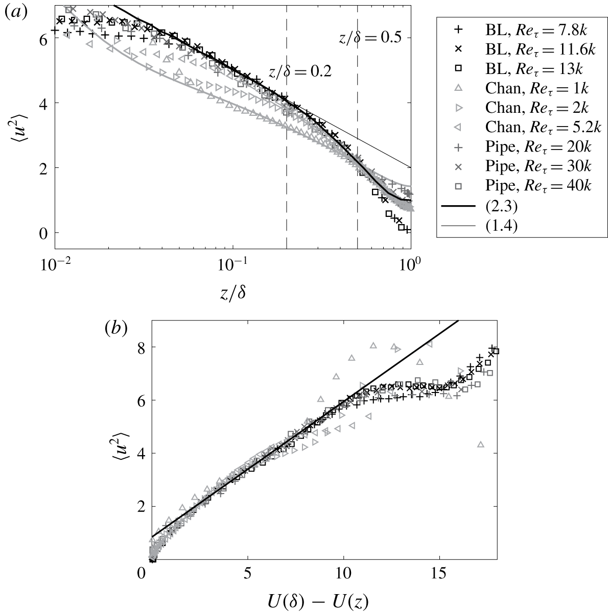
(Data in the neutral stability regime) (a) The variance of the streamwise velocity fluctuation in neutral boundary layers, pipes and channels. The best fit according to (2.3) yields  $C_{1}\approx 0.5$,
 $C_{2}\approx 0.9$ for boundary-layer data,
 $C_{1}\approx 0.5$,
 $C_{2}\approx 1.4$ for pipe data, and
 $C_{1}\approx 0.41$,
 $C_{2}\approx 1.43$ for the channel at
 $Re_{\unicode[STIX]{x1D70F}}=1000$. ‘BL’ stands for ‘boundary layer’. ‘Chan’ stands for ‘channel flow’. The letter ‘
 $k$’ denotes
 $\times 10^{3}$. Velocities are normalized using
 $u_{\unicode[STIX]{x1D70F}}$. (b) The velocity variance as a function of
 $U(\unicode[STIX]{x1D6FF})-U(z)$. The pipe data are displaced vertically to account for the non-zero velocity fluctuation near the pipe centreline.

Figure 1(a) shows both  $\langle u^{2}\rangle$ and
 $C_{1}[U(\unicode[STIX]{x1D6FF})-U(z)]+C_{2}$, as a function of
 $z/\unicode[STIX]{x1D6FF}$ for neutral boundary-layer flows at
 $Re_{\unicode[STIX]{x1D70F}}$ from 7800 to 13 000, pipe flow at
 $Re_{\unicode[STIX]{x1D70F}}$ from
 $20\,000$ to
 $40\,000$ (Örlü et al. Reference Örlü, Fiorini, Segalini, Bellani, Talamelli and Alfredsson2017) and channel flow from
 $Re_{\unicode[STIX]{x1D70F}}=1000$ to
 $5200$ (Lee & Moser Reference Lee and Moser2015; Graham et al. Reference Graham, Kanov, Yang, Lee, Malaya, Lalescu, Burns, Eyink, Szalay, Moser and Meneveau2016). The boundary-layer data are hot-wire measurements from the Melbourne high-Reynolds-number boundary-layer wind tunnel (known as the HRNBLWT). Details of the measurements can be found in Hutchins et al. (Reference Hutchins, Nickels, Marusic and Chong2009) and Talluru et al. (Reference Talluru, Baidya, Hutchins and Marusic2014). The pipe flow data are measurements from the Bologna Centre for International Cooperation in Long Pipe Experiments (known as CICLoPE). Details of the facility can be found in Örlü et al. (Reference Örlü, Fiorini, Segalini, Bellani, Talamelli and Alfredsson2017). The channel flow data are publicly available through the Johns Hopkins Turbulence Data Base and the UT turbulence data base, and details of the direct numerical simulations (DNS) may be found in Lee & Moser (Reference Lee and Moser2015) and Graham et al. (Reference Graham, Kanov, Yang, Lee, Malaya, Lalescu, Burns, Eyink, Szalay, Moser and Meneveau2016). Equation (1.4) fits
 $\langle u^{2}\rangle$ in the log layer at high Reynolds numbers. The boundary layers and the pipe flows are at fairly high Reynolds numbers, and in figure 1(a), the data follow (1.4) reasonably well in the log layer (although the extent of the log layer is limited). The channel flow data are at moderate Reynolds numbers, and (1.4) does not provide good fits of
 $\langle u^{2}\rangle$ at
 $Re_{\unicode[STIX]{x1D70F}}=1000$ and
 $Re_{\unicode[STIX]{x1D70F}}=2000$. This limits the use of (1.4) to flows at only high Reynolds numbers. Figure 1(b) shows
 $\langle u^{2}\rangle$ as a function of
 $U(\unicode[STIX]{x1D6FF})-U(z)$, and (2.3) provides good fits for
 $\langle u^{2}\rangle$ at both high and moderate Reynolds numbers.
We discuss why (2.3) fits the data better than (1.4) at moderate Reynolds numbers. Equation (1.4) holds only if the eddies are wall attached and space filling. In the wake layer (i.e. above the logarithmic layer), the eddies may still be wall attached but are by no means space filling (Krug et al. Reference Krug, Philip and Marusic2017; Xu & Yang Reference Xu and Yang2018). In fact, because of free-stream (or quiescent core) intrusions, (part of) the wake layer in boundary layers (channels) is intermittently turbulent and laminar. Hence, from a statistical perspective, eddies in the wake layer only fill part of the available space. A straightforward measure of the space fillingness is the fractal dimension of the eddies in the wake layer, which was measured and reported in Xu & Yang (Reference Xu and Yang2018) for flows at different Reynolds numbers. In their analysis, Xu & Yang (Reference Xu and Yang2018) concluded that non-space fillingness yields deviations from the logarithmic law of the wall in the wake layer, and that the fractal dimension of the flow in the wake layer directly relates to the parameterization of the wake profile. Here, a consequence of eddies being non-space filling is that the eddy population density  $P(z)<1/z$ in the wake layer, and
 $$\begin{eqnarray}\langle u^{2}\rangle \sim \int _{z}^{\unicode[STIX]{x1D6FF}}P(z^{\prime })\,\text{d}z^{\prime }<\int _{z}^{\unicode[STIX]{x1D6FF}}\frac{1}{z^{\prime }}\,\text{d}z^{\prime }\sim \log (\unicode[STIX]{x1D6FF}/z),\end{eqnarray}$$
i.e. leading to the failure of (1.4). At a moderate Reynolds number, say,  $Re_{\unicode[STIX]{x1D70F}}=1000$, the flow at
 $z^{+}=100$ is already in the wake layer, hence (1.4) does not work well at moderate Reynolds numbers. However, because (2.3) connects
 $\langle u^{2}\rangle$ and
 $U$ through the eddy population density, one still has
 $$\begin{eqnarray}\langle u^{2}\rangle \sim \int _{z}^{\unicode[STIX]{x1D6FF}}P(z^{\prime })\,\text{d}z^{\prime }\sim U_{\infty }^{+}-U^{+},\end{eqnarray}$$
both in the wake and in the logarithmic layers.
From a practical standpoint, both (1.4) and (2.3) have two constants that must be determined. Compared to (1.4), which is a good fit of  $\langle u^{2}\rangle$ from
 $z^{+}\approx 3.5\sqrt{Re_{\unicode[STIX]{x1D70F}}}$ to
 $z/\unicode[STIX]{x1D6FF}\approx 0.2$, (2.3) is a good fit up to
 $z/\unicode[STIX]{x1D6FF}\approx 0.5$ (see figure 1a). Moreover, according to figure 1(b), (2.3) provides good fits for
 $\langle u^{2}\rangle$ at both moderate and high Reynolds numbers, whereas (1.4) is only valid at high Reynolds number. This is quite useful. Using (2.3), we could study the scaling behaviours of flow statistics at moderate Reynolds numbers, which would not be possible using (1.4). We fit for
 $C_{1}$ and
 $C_{2}$ in the log layer, i.e. from
 $z^{+}=3.5\sqrt{Re_{\unicode[STIX]{x1D70F}}}$ to
 $z/\unicode[STIX]{x1D6FF}=0.4\sim 0.5$, using the high-Reynolds-number data. The measured value is
 $C_{1}=0.5$ and the value agrees with (3.1). Although (2.3) fits the data at moderate Reynolds numbers, the limited extent of the log layer affects the measurement of the two constants
 $C_{1}$,
 $C_{2}$ (Stevens, Wilczek & Meneveau Reference Stevens, Wilczek and Meneveau2014), leading to uncertainties in the measured constants. In anticipation of the results in the next subsection, we note that the uncertainty in the measured
 $C_{1}$ at a Reynolds number
 $Re_{\unicode[STIX]{x1D70F}}\approx 1000$ is approximately
 $0.1$.
Figure 1(a) shows the wall-normal extent in which (2.3) is valid, and is therefore more informative than figure 1(b). In the following, we will focus on the velocity variance as a function of the wall-normal height, and we will compare (2.3) to the data up to  $z/\unicode[STIX]{x1D6FF}\approx 0.4$.
3.2 Weakly unstable boundary-layer flows
Next, we compare the proposed scaling to weakly unstable boundary-layer flow data, namely  $L/\unicode[STIX]{x1D6FF}\lesssim -1$. Because of the prohibitive computational cost, direct numerical simulation of weakly unstable boundary layers is only currently feasible available at moderate Reynolds numbers. DNS of weakly unstable flows at moderate Reynolds numbers can be found in, e.g. Domaradzki & Metcalfe (Reference Domaradzki and Metcalfe1988), Garai, Kleissl & Sarkar (Reference Garai, Kleissl and Sarkar2014) and Pirozzoli et al. (Reference Pirozzoli, Bernardini, Verzicco and Orlandi2017). In the present study, some data from the latter paper are used. The incompressible Navier–Stokes equations are solved under the Boussinesq approximation in a periodic plane channel, with half-height
 $\unicode[STIX]{x1D6FF}$ and wall-parallel size
 $16\unicode[STIX]{x1D6FF}\times 8\unicode[STIX]{x1D6FF}$ in the streamwise and spanwise directions, respectively. The flow is controlled by the friction Reynolds number,
 $Re_{\unicode[STIX]{x1D70F}}$, the molecular Prandtl number
 $Pr$ (assumed to be unity), and
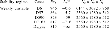
 $L/\unicode[STIX]{x1D6FF}$, i.e. the ratio of the MO length and the half-channel height. Details on the DNS parameters used for the analysis are given in table 1, where each flow case is denoted as
 $L$ followed by the respective value of
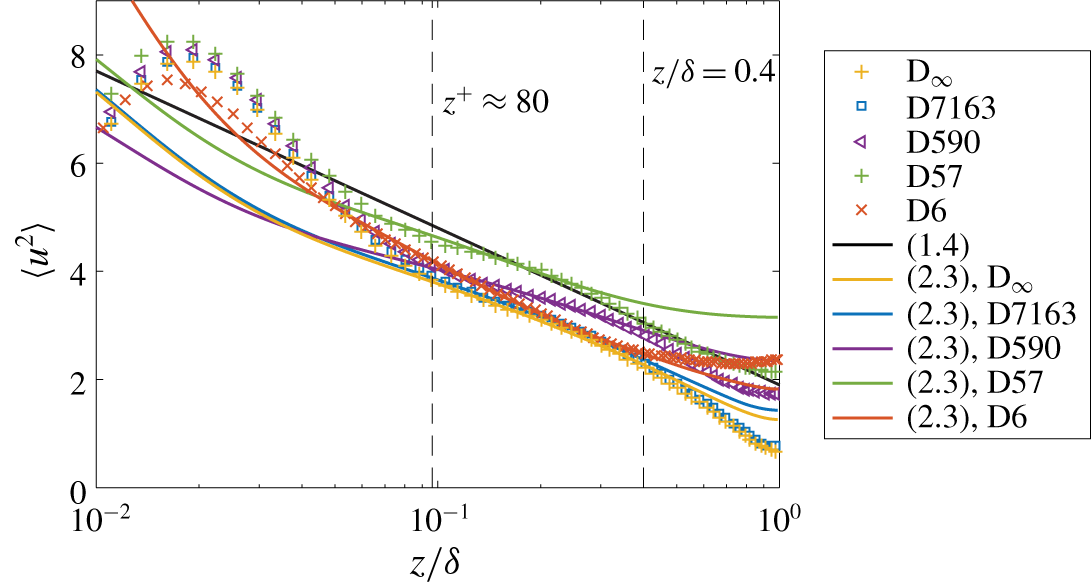
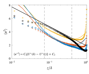
 $L/\unicode[STIX]{x1D6FF}$. Figure 2 shows the DNS data and
 $C_{1}[U(\unicode[STIX]{x1D6FF})-U(z)]+C_{2}$. For weakly unstable boundary layers, stratification does not seem to affect the flow statistics for
 $L/\unicode[STIX]{x1D6FF}<-60$. Again, because of the finite Reynolds number, (1.4) does not fit the
 $\text{L}_{\infty }$ flow case (note, at high Reynolds number,
 $\langle u^{2}\rangle$ should follow (1.4)). For
 $L/\unicode[STIX]{x1D6FF}<-0.6$, (2.3) well fits the streamwise velocity fluctuations for
 $80<z^{+}$,
 $z/\unicode[STIX]{x1D6FF}<0.4$.
The streamwise velocity variance in weakly unstable channels. Details of the data are tabulated in table 1. The cases are colour coded. The solid lines are  $C_{1}[U(\unicode[STIX]{x1D6FF})-U(z)]+C_{2}$. The two constants are best fits of the data for
 $z^{+}<80$,
 $z/\unicode[STIX]{x1D6FF}<0.4$. For
 $\text{D}_{\infty }$, D7163, D590, D57 and D6,
 $C_{1}=0.41$, 0.41, 0.31, 0.40, 0.85 and
 $C_{2}=1.3$,
 $1.4$,
 $2.3$,
 $3.2$,
 $1.8$, respectively. Because of the limited Reynolds number and the resulting limited extent of the inertial layer, there is an uncertainty of approximately 0.1 in the measured
 $C_{1}$ values. The scaling for a neutral boundary layer is included for reference.

Details of DNS of weakly unstable channel flow (Pirozzoli et al. Reference Pirozzoli, Bernardini, Verzicco and Orlandi2017).  $Re_{\unicode[STIX]{x1D70F}}=u_{\unicode[STIX]{x1D70F}}\unicode[STIX]{x1D6FF}/\unicode[STIX]{x1D708}$ is the friction Reynolds number.
 $N_{x}$,
 $N_{y}$ and
 $N_{z}$ are the grid in the streamwise, spanwise and wall-normal directions.

3.3 Unstable boundary-layer flows
Last, we compare the model to unstable boundary-layer flows, namely,  $-1\lesssim L/\unicode[STIX]{x1D6FF}<-0.1$. DNS of boundary-layer flows with strong stratification are prohibitively costly even at moderate Reynolds numbers, and therefore we resort to the more cost effective tool of large-eddy simulation (LES). LES is very commonly used for studying thermally stratified boundary-layer flows (Huang & Bou-Zeid Reference Huang and Bou-Zeid2013; Katul et al. Reference Katul, Li, Chamecki and Bou-Zeid2013; Stevens et al. Reference Stevens, Wilczek and Meneveau2014). Our LES code has been extensively utilized for thermally stratified boundary-layer flow simulations (see, e.g. Stoll & Porté-Agel (Reference Stoll and Porté-Agel2009), Abkar, Sharifi & Porté-Agel (Reference Abkar, Sharifi and Porté-Agel2016), Abkar, Sørensen & Porté-Agel (Reference Abkar, Sørensen and Porté-Agel2018)). It solves the filtered incompressible Navier–Stokes equations, under the Boussinesq approximation, and the filtered transport equation for the potential temperature in a half-channel,
 $$\begin{eqnarray}\displaystyle & \displaystyle \unicode[STIX]{x2202}_{i}\widetilde{U}_{i}=0, & \displaystyle\end{eqnarray}$$
 $$\begin{eqnarray}\displaystyle & \displaystyle \unicode[STIX]{x2202}_{t}\widetilde{U}_{i}+\unicode[STIX]{x2202}_{j}(\widetilde{U}_{i}\widetilde{U}_{j})=-\frac{1}{\unicode[STIX]{x1D70C}}\unicode[STIX]{x2202}_{i}\widetilde{P}+\unicode[STIX]{x2202}_{j}(\unicode[STIX]{x1D708}\unicode[STIX]{x2202}_{j}\widetilde{U}_{i})-\unicode[STIX]{x2202}_{j}\unicode[STIX]{x1D70F}_{ij}+\unicode[STIX]{x1D6FF}_{i3}g\frac{\widetilde{\unicode[STIX]{x1D6E9}}-\overline{\widetilde{\unicode[STIX]{x1D6E9}}}}{\unicode[STIX]{x1D6E9}_{0}}+F_{p}\unicode[STIX]{x1D6FF}_{i1}, & \displaystyle\end{eqnarray}$$
 $$\begin{eqnarray}\displaystyle & \displaystyle \unicode[STIX]{x2202}_{t}\widetilde{\unicode[STIX]{x1D6E9}}+\unicode[STIX]{x2202}_{i}(\widetilde{U}_{i}\widetilde{\unicode[STIX]{x1D6E9}})=\unicode[STIX]{x2202}_{i}({\mathcal{D}}\unicode[STIX]{x2202}_{i}\widetilde{\unicode[STIX]{x1D6E9}})-\unicode[STIX]{x2202}_{i}q_{i}+S_{\unicode[STIX]{x1D703}}, & \displaystyle\end{eqnarray}$$
 $\widetilde{U}_{i}$ is the resolved velocity, and
 $i=1$,
 $2$ and
 $3$ respectively represent the streamwise (
 $x$), spanwise (
 $y$) and wall-normal (
 $z$) directions. Time is denoted with
 $t$;
 $\widetilde{P}$ is the filtered pressure;
 $\unicode[STIX]{x1D70C}$ and
 $\unicode[STIX]{x1D708}$ are the fluid density and kinematic viscosity, respectively; and
 ${\mathcal{D}}$ is the molecular diffusivity;
 $\widetilde{\unicode[STIX]{x1D6E9}}$ is the resolved potential temperature;
 $\unicode[STIX]{x1D70F}_{ij}=\widetilde{U_{i}U_{j}}-\widetilde{U}_{i}\widetilde{U}_{j}$ is the subgrid-scale (SGS) stress tensor; and
 $q_{i}=\widetilde{U_{i}\unicode[STIX]{x1D6E9}}-\widetilde{U}_{i}\widetilde{\unicode[STIX]{x1D6E9}}$ is the SGS heat flux. The parameter
 $F_{p}$ is an imposed uniform pressure gradient;
 $S_{\unicode[STIX]{x1D703}}$ represents a suitable source term for the potential temperature (Kim & Moin Reference Kim and Moin1989; Pirozzoli, Bernardini & Orlandi Reference Pirozzoli, Bernardini and Orlandi2016);
 $\unicode[STIX]{x1D6E9}_{0}$ is the reference temperature;
 $\unicode[STIX]{x1D6FF}_{ij}$ is the Kronecker delta tensor; and the overline denotes horizontal averaging. The SGS turbulent fluxes are modelled using the Lagrangian scale-dependent dynamic model (LSDM) (Bou-Zeid, Meneveau & Parlange Reference Bou-Zeid, Meneveau and Parlange2005; Stoll & Porté-Agel Reference Stoll and Porté-Agel2006) and the anisotropic minimum dissipation model (AMD) (for L4-sgs only) (Rozema et al. Reference Rozema, Bae, Moin and Verstappen2015; Abkar, Bae & Moin Reference Abkar, Bae and Moin2016; Abkar & Moin Reference Abkar and Moin2017). The wall shear and the surface heat flux are specified according to the equilibrium wall model including the effects of surface stratification (Moeng Reference Moeng1984; Yang, Park & Moin Reference Yang, Park and Moin2017),
 $$\begin{eqnarray}\displaystyle & \displaystyle \left.\begin{array}{@{}c@{}}\displaystyle \unicode[STIX]{x1D70F}_{w,x}=-\left[\frac{\unicode[STIX]{x1D705}\widetilde{U}_{\Vert }}{\text{log}(\unicode[STIX]{x0394}z/z_{o})+\unicode[STIX]{x1D713}_{M}(\unicode[STIX]{x0394}z/L)}\right]^{2}\frac{\widetilde{U}_{\unicode[STIX]{x1D6E5}}}{U_{\Vert }},\\ \displaystyle \unicode[STIX]{x1D70F}_{w,y}=-\left[\frac{\unicode[STIX]{x1D705}\widetilde{U}_{\Vert }}{\text{log}(\unicode[STIX]{x0394}z/z_{o})+\unicode[STIX]{x1D713}_{M}(\unicode[STIX]{x0394}z/L)}\right]^{2}\frac{\widetilde{V}_{\unicode[STIX]{x1D6E5}}}{U_{\Vert }},\end{array}\right\} & \displaystyle\end{eqnarray}$$
 $$\begin{eqnarray}\displaystyle & \displaystyle q_{w,z}=\left[\frac{\unicode[STIX]{x1D705}\widetilde{U}_{\Vert }}{\text{log}(\unicode[STIX]{x0394}z/z_{o})+\unicode[STIX]{x1D713}_{M}(\unicode[STIX]{x0394}z/L)}\right]\left[\frac{\unicode[STIX]{x1D705}(\unicode[STIX]{x1D6E9}_{s}-\widetilde{\unicode[STIX]{x1D6E9}}_{\unicode[STIX]{x1D6E5}})}{\text{log}(\unicode[STIX]{x0394}z/z_{o})+\unicode[STIX]{x1D713}_{H}(\unicode[STIX]{x0394}z/L)}\right], & \displaystyle\end{eqnarray}$$
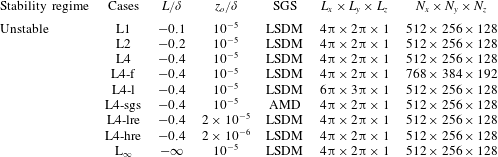
Details of the LES of unstable channel flow (except for  $\text{L}_{\infty }$, which is neutral).
 $L_{x}$,
 $L_{y}$ and
 $L_{z}$ are the streamwise (
 $x$), spanwise (
 $y$) and wall-normal (
 $z$) extents of the computational domain.
 $N_{x}$,
 $N_{y}$ and
 $N_{z}$ are the grid in the
 $x$,
 $y$ and
 $z$ directions.
 $z_{o}$ is the effective ground roughness height.
 $\unicode[STIX]{x1D6FF}/z_{o}$ is the ratio of the sizes of the biggest eddy and the smallest eddy in the flow and therefore may be interpreted as the Reynolds number.

where  $\unicode[STIX]{x1D70F}_{w,x/y}$ is the wall-shear stress in the streamwise and the spanwise directions, and
 $q_{w,z}$ is the wall-heat flux;
 $\widetilde{U}_{\unicode[STIX]{x1D6E5}}$,
 $\widetilde{V}_{\unicode[STIX]{x1D6E5}}$ and
 $\widetilde{\unicode[STIX]{x1D6E9}}_{\unicode[STIX]{x1D6E5}}$ are the temporally filtered LES velocity and temperature, respectively, at a distance
 $\unicode[STIX]{x0394}z$ from the wall,
 $\unicode[STIX]{x0394}z$ is the height of the first off-wall grid,
 $z_{o}$ is a roughness/viscous length scale and
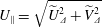 $U_{\Vert }=\sqrt{\widetilde{U}_{\unicode[STIX]{x1D6E5}}^{2}+\widetilde{V}_{\unicode[STIX]{x1D6E5}}^{2}}$ is the wall-parallel velocity;
 $\unicode[STIX]{x1D6E9}_{s}$ is the surface temperature, and it is kept constant in time. Here,
 $\unicode[STIX]{x1D713}_{M}$ and
 $\unicode[STIX]{x1D713}_{H}$ are the stability correction functions for momentum and heat, here implemented in the classical form suggested by Businger et al. (Reference Businger, Wyngaard, Izumi and Bradley1971). The molecular viscosity is set to zero away from the wall, hence the flow is at nominally infinite Reynolds number. Further details of the solver may be found in Abkar & Porté-Agel (Reference Abkar and Porté-Agel2015) and Yang & Abkar (Reference Yang and Abkar2018). The simulation set-up of the LES are summarized in table 2. In this study, we have imposed an isothermal boundary condition at the wall. If a constant heat flux was imposed at the wall instead, temperature would not be statistically stationary, thus making it complicated to analyse its statistics, whereas velocity would still reach a statistically stationary state. All the flow statistics are averaged in the two homogeneous directions and in time for approximately twenty flow-through times after the flow reaches a statistically stationary state, with one flow through corresponding to
 $t=L_{x}/u_{b}$, and
 $u_{b}$ is the bulk velocity. For the L4 flow case, LES are carried out with a finer resolution (L4-f), in a larger computational domain (L4-l), using a different SGS model (L4-sgs), at a nominally higher and lower Reynolds number (L4-hre and L4-lre). In neutral smooth-wall boundary-layer flows, the parameter
 $z_{o}$ in the wall model is directly related to the viscosity as
 $$\begin{eqnarray}z_{o}=\frac{\unicode[STIX]{x1D708}}{u_{\unicode[STIX]{x1D70F}}}\exp (-\unicode[STIX]{x1D705}B),\end{eqnarray}$$
and the friction Reynolds number is related to  $z_{o}$ and
 $\unicode[STIX]{x1D6FF}$ through
 $$\begin{eqnarray}Re_{\unicode[STIX]{x1D70F}}=\frac{\unicode[STIX]{x1D6FF}}{z_{o}}\exp (-\unicode[STIX]{x1D705}B).\end{eqnarray}$$
In this sense, decreasing or increasing  $z_{o}$ is similar to increasing or decreasing the Reynolds number. Hence L4-lre and L4-hre are at a nominally lower and higher Reynolds number than L4. The streamwise velocity fluctuation is no different from that in L4 (and therefore not shown here for brevity). Hence, for the rest of the LES, we use the same resolution, domain size, SGS model and roughness height as L4. In addition to unstable boundary-layer flows, we also conduct an LES of a neutral boundary-layer flow for reference and code validation purposes.
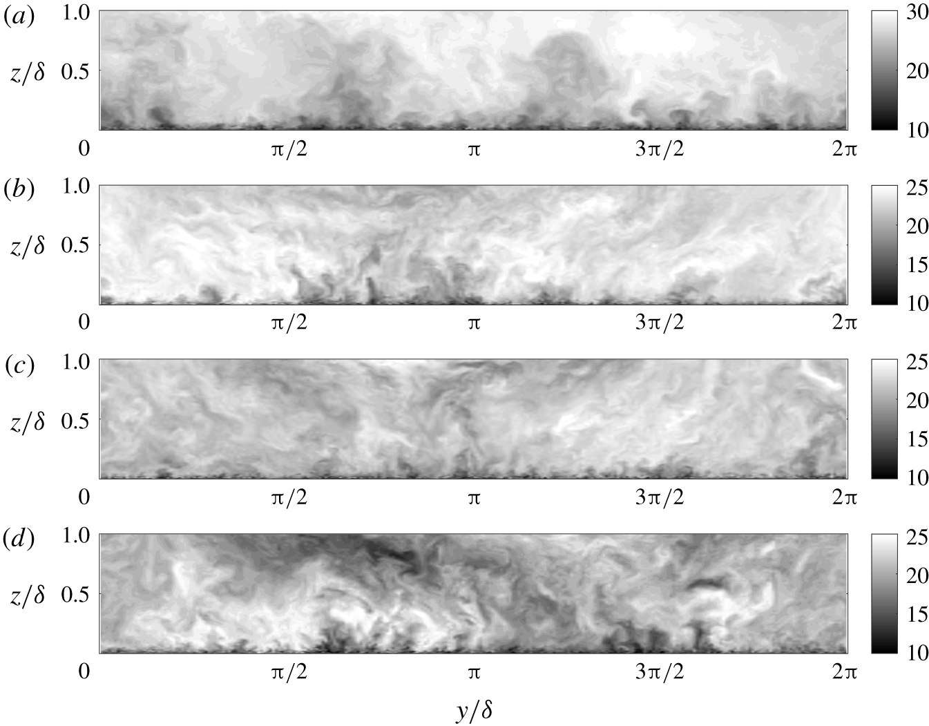
Instantaneous streamwise velocity contours on spanwise/wall-normal planes from  $\text{L}_{\infty }$ (a), L4 (b), L2 (c) and L1 (d). The velocity is normalized using the friction velocity.

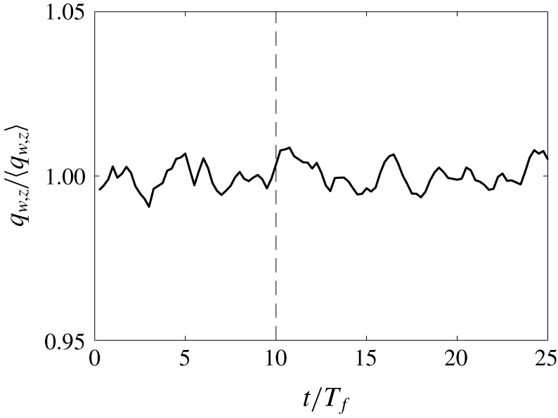
Figure 3 shows the instantaneous streamwise velocity contours in a spanwise wall-normal plane cut from  $\text{L}_{\infty }$ (a), L4 (b), L2 (c) and L1 (d). Although turbulence in unstable boundary layers appears to be more vigorous, the instantaneous flow fields are not qualitatively different: the eddies are larger sized away from the wall than those near the wall. Figure 4 shows the horizontally averaged wall-heat flux as a function of time in L1 for the last 25 flow-through times of our simulation. Because of the large computational domain, the horizontally averaged flux varies weakly in time (less than
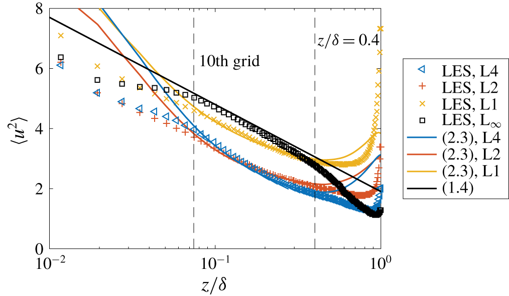
 $\pm 1\,\%$). Time variations of the wall-heat flux in L2 and L4 are similar and are not shown here for brevity. Figure 5 shows the streamwise velocity variance as a function of the wall-normal distance. Again, for the cases shown here, near-wall turbulence fluctuations (in wall units) are weaker in unstable boundary-layer flows than in a neutral boundary-layer flow, although the turbulence level (normalized by the incoming velocity) is higher in unstable boundary-layer flows because of the reduced mean flow. The near-wall turbulence is not well resolved (Kawai & Larsson Reference Kawai and Larsson2012), and therefore only the data above the tenth grid point are compared to the model. For the neutral flow, our LES follows (1.4) in the log layer (up to approximately
 $z/\unicode[STIX]{x1D6FF}\approx 0.2$). For flows that are statistically unstable, the streamwise velocity fluctuation does not scale logarithmically, and only (2.3) provides a good fit to the data from the tenth grid point to
 $z/\unicode[STIX]{x1D6FF}\approx 0.4$.
Horizontally averaged wall-heat flux as a function of time in L1.  $T_{f}$ is one flow-through time.


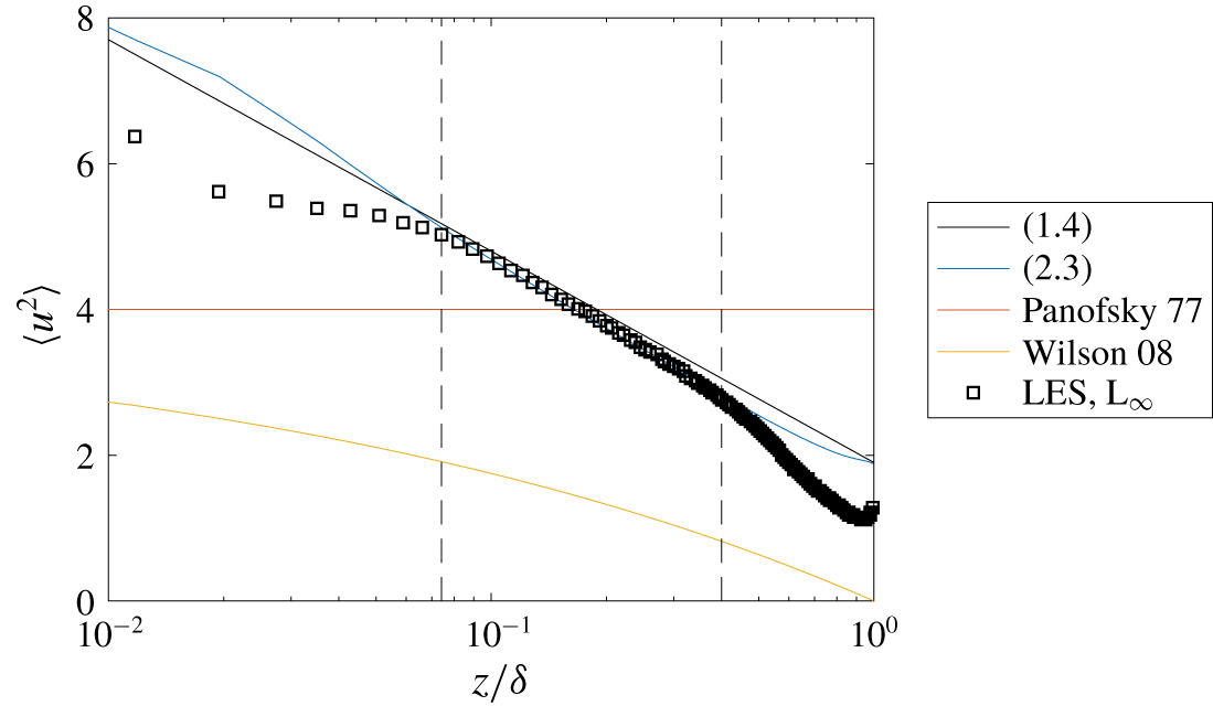
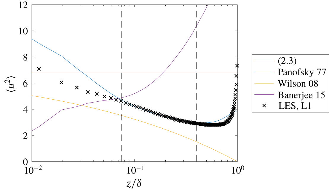
Last, we compare (2.3) and some of the scalings in the literature, i.e. (1.8), (1.9) and (1.10), for  $-L=\infty$ and
 $-L/\unicode[STIX]{x1D6FF}=0.1$. Figures 6 and 7 show the comparison for
 $-L=\infty$ and
 $-L=0.1$, respectively. Equation (2.3) conforms with (1.4) at the neutral condition and fits the data well at both the neutral condition and the unstable condition. Equations (1.8), (1.9) and (1.10) are somewhat off. It is worth noting that this comparison is not entirely fair, as expressing a flow quantity in terms of another flow quantity is usually much simpler than as a function of independent time and space variables (Yang et al. Reference Yang, Meneveau, Marusic and Biferale2016).




3.4 Fit constants
The main emphasis of this work is establishing the general validity of the scaling (2.3), but of course a priori prescription of suitable values for the two constants  $C_{1}$ and
 $C_{2}$ in (2.3) is quite important from a practical standpoint. In the case of neutral flows, the two constants are given in (3.1), according to which
 $C_{1}\equiv 0.5$, whereas
 $C_{2}$ may be flow dependent. Following the same argument that led to the MO similarity theory, for statistically unstable flows, both
 $C_{1}$ and
 $C_{2}$ are expected to be functions of the flow stratification, i.e.
 $L/\unicode[STIX]{x1D6FF}$, but should not change at sufficiently high Reynolds numbers.
First, we consider the  $C_{2}$ constant. Following the same argument that led to the conclusion that the coefficient
 $B_{1}$ in (1.4) is flow dependent (Marusic et al. Reference Marusic, Monty, Hultmark and Smits2013), we may conclude that
 $C_{2}$ must depend on velocity fluctuations at the boundary-layer height/channel centreline/pipe centreline, and therefore it is not universal, as was probably already clear from (3.1). Next, we consider
 $C_{1}$, which should solely be a function of the flow stratification parameter,
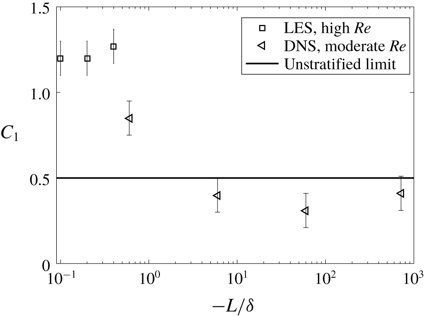
 $L/\unicode[STIX]{x1D6FF}$. Figure 8 shows the value of
 $C_{1}$ obtained from data fit as a function of
 $L/\unicode[STIX]{x1D6FF}$. The uncertainty in the LES measured values is mainly due to the under-resolved near-wall region, as thoroughly discussed in Stevens et al. (Reference Stevens, Wilczek and Meneveau2014). On the other hand, uncertainty in the DNS measured values is due to our choice of the extent of the wall-normal distance range within which the proposed scaling is valid. This is similar to the classical problem of determining the log-law constants by fitting mean velocity profiles (Nagib & Chauhan Reference Nagib and Chauhan2008). Following the discussion in § 3, the uncertainty is approximately
 $\pm 0.1$. For a statistically unstable boundary layer, the constant
 $C_{1}$ is an increasing function of the flow stratification, and the limited data seem to suggest that
 $C_{1}\equiv 1.2$ for unstable boundary layers.
The fit constant  $C_{1}$ as a function of
 $L/\unicode[STIX]{x1D6FF}$.

4 Concluding remarks
This work builds on the classical MO similarity theory and Townsend’s attached-eddy hypothesis, on whose basis we propose a scaling that connects the mean flow to the streamwise velocity variance in statistically unstable boundary layers, as embodied by (2.3). To summarize, we start by allowing flow stratification to change the local eddy size and the local eddy population density; consequently, known scaling laws that fit the turbulent statistics in a neutral boundary-layer flow do not fit the same statistics in a statistically unstable flow. Compared to (1.4), which is a good working approximation of  $\langle u^{2}\rangle$ from
 $z^{+}\approx 3.5\sqrt{Re_{\unicode[STIX]{x1D70F}}}$ to
 $z\approx 0.2\unicode[STIX]{x1D6FF}$ in neural boundary layers at high Reynolds numbers, (2.3) provides reasonably good fits for
 $\langle u^{2}\rangle$ from
 $z^{+}\approx 3.5\sqrt{Re_{\unicode[STIX]{x1D70F}}}$ up to
 $z\approx 0.5\unicode[STIX]{x1D6FF}$ in both neural and statistically unstable boundary layer flows at both moderate and high Reynolds numbers. This is quite useful because it allows one to study the scaling behaviours of flow statistics at DNS accessible moderate Reynolds numbers.
To conclude, we briefly discuss potential applications of (2.3) (or equivalently (2.4)). Measurements of mean and fluctuating wind in wind farms are typically available at only a few heights. Using measurements at two (or a few more) heights, the unknown constants  $C_{1}$ and
 $C_{2}$ in (2.3) (or
 $C_{1}$ and
 $C_{2}^{\prime }$ in (2.4)) can be determined, thus allowing us to infer the whole distribution of velocity fluctuations in and above a wind farm from the mean flow. Although
 $C_{1}$ and
 $C_{2}$ can be empirically determined based on the above procedure, available data suggest that
 $C_{1}=1.2\sim 1.3$ is universal for highly unstable flows at high Reynolds numbers, a speculation that will need more data to confirm/refute and is left for future investigation.
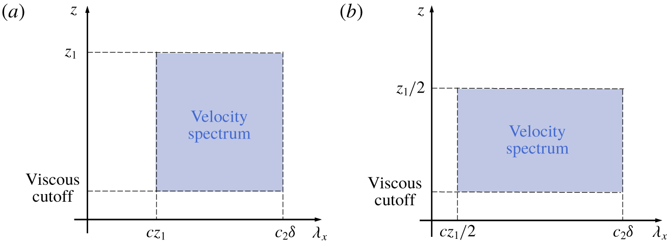
(a) Schematic of the pre-multiplied velocity spectrum due to wall-attached eddies of size  $z_{1}$. (b) Same as (a) but for eddies of size
 $z_{1}/2$. Both axes are in logarithmic scale.

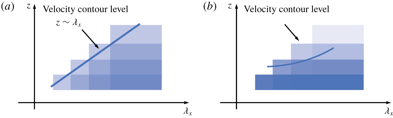
(a) Schematic of the pre-multiplied velocity spectrum of a boundary-layer flow. We assume that the eddies are wall-attached, self-similar and space filling. (b) Same as (a), but eddies are not space filling.

Acknowledgements
The work is financially supported by the Penn State University and Aarhus University. We further acknowledge that the DNS results have been achieved using the PRACE Research Infrastructure resource MARCONI based at CINECA, Casalecchio di Reno, Italy.
Declaration of interests
The authors report no conflict of interest.
Appendix A. Eddy population density and pre-multiplied energy spectrum
In this section, we make a connection between the eddy population density function and the scaling of the pre-multiplied energy spectrum. The discussion follows from Baars, Hutchins & Marusic (Reference Baars, Hutchins and Marusic2017) and Baars & Marusic (Reference Baars and Marusic2020). In particular, we will show that the eddy population density function in an unstably stratified boundary-layer flow does not scale as  ${\sim}1/z$. This analysis is rather standard, hence we will only go through the main steps. Figure 9(a) sketches the pre-multiplied energy spectrum due to wall-attached eddies of size
 $z_{1}$. The spectrum spans the wall-normal axis from a viscous cutoff to
 $z_{1}$ and the streamwise axis from
 $cz_{1}$ to
 $c_{2}\unicode[STIX]{x1D6FF}$, where
 $c$ and
 $c_{2}$ are constants. The pre-multiplied velocity spectrum due to wall-attached eddies of size
 $z_{1}/2$ is sketched in figure 9(b). Assuming that the eddy population density is
 ${\sim}1/z$, the spectra in figure 9(a,b) are of the same magnitudes. Superposition of these spectra yields the velocity spectrum of the flow. Figure 10(a) is a sketch of the superimposed velocity spectrum. The contour levels scale as
 $z\sim \unicode[STIX]{x1D706}_{x}$. In a nutshell, if the eddy population density is
 ${\sim}1/z$, in the logarithmic layer, the contours of the velocity spectrum scale as
 $z\sim \unicode[STIX]{x1D706}_{x}$. It is worth noting that the sketched spectrum is solely due to wall-attached eddies. The inner peak is due to viscous scales, and is located southwest of the sketched spectrum. The outer peak in the spectrum is due to large-scale structure, very large-scale structures and superstructures, and is located to the east of the sketched spectrum.
Next, we model the pre-multiplied spectrum for an eddy population density function that does not scale as  ${\sim}1/z$. In this case, the spectrum due to eddies of size
 $z_{1}$ will be different from that of eddies of size
 $z_{1}/2$ in terms of their magnitudes. Consequently, the contours do not scale as
 $z\sim \unicode[STIX]{x1D706}_{x}$, as sketched in figure 10(b). The precise scaling of the contours depends on the scaling of the eddy population density function. Specifically, at a height
 $z$,
 $$\begin{eqnarray}\frac{\text{available space}}{\text{eddy population density}}\sim \text{space occupied by one eddy},\end{eqnarray}$$
where the available space at a height  $z$ is proportional to ‘
 $\text{unit horizontal area}\times z$’, the eddy population density is proportional ‘
 $\unicode[STIX]{x1D719}_{M}/z$’ and the space occupied by one turbulent eddy is ‘
 $\unicode[STIX]{x1D706}_{x}\times z$’, where
 $\unicode[STIX]{x1D706}_{x}$ is the characteristic length of an eddy in the streamwise direction. Hence, equation (A 1) is
 $$\begin{eqnarray}\frac{z}{\unicode[STIX]{x1D719}_{M}/z}\sim \unicode[STIX]{x1D706}_{x}\times z,\end{eqnarray}$$
which directly leads to  $\unicode[STIX]{x1D706}_{x}\sim z/\unicode[STIX]{x1D719}_{M}$, or equivalently,
 $z\sim \unicode[STIX]{x1D719}_{M}\unicode[STIX]{x1D706}_{x}$ (up to constants). For eddies that are space filling,
 $\unicode[STIX]{x1D719}_{M}=1$ and
 $\unicode[STIX]{x1D706}_{x}\sim z$, conforming to the attached-eddy hypothesis.
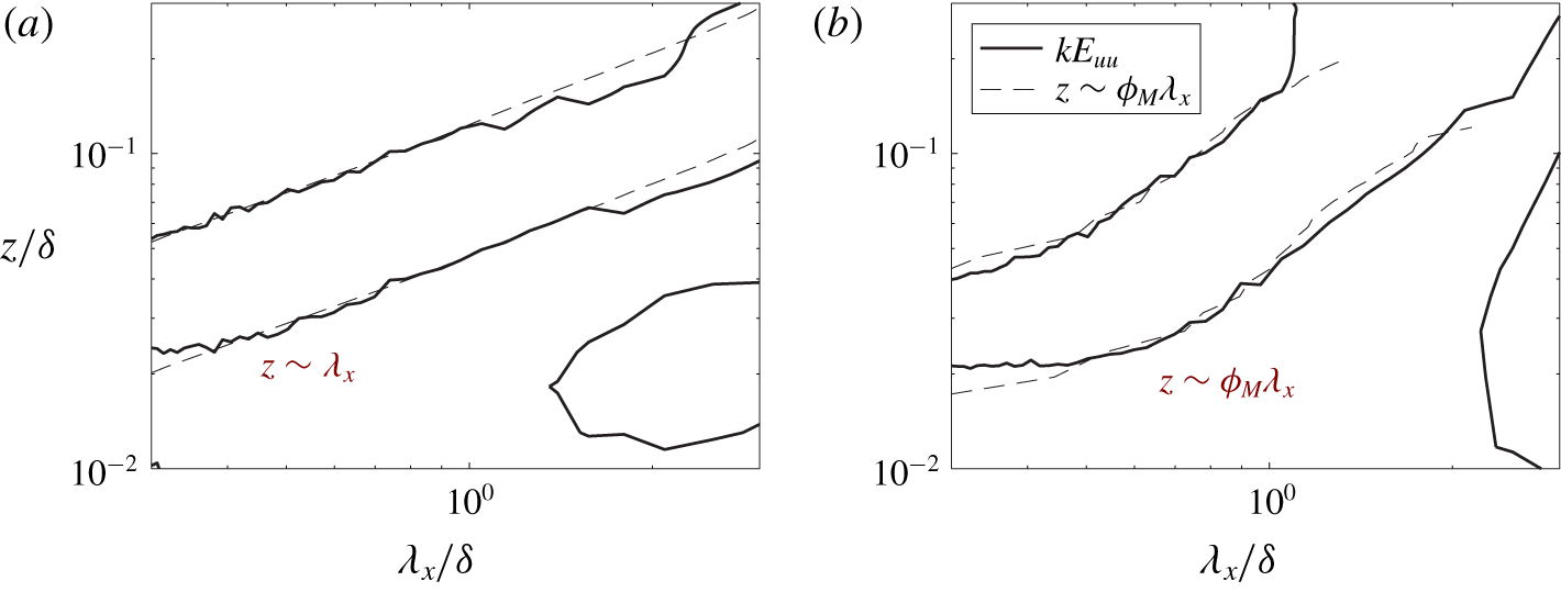
Now we show data of the pre-multiplied energy spectra in neutral boundary-layer flow (figure 11a) and in unstably boundary-layer flow (figure 11b). Following Baars & Marusic (Reference Baars and Marusic2020), we only focus on the relevant part of the spectrum. The contours scale as  $z\sim x$ at a neutral condition, whereas at a unstable condition the contour levels scale as
 $z\sim \unicode[STIX]{x1D719}_{M}\unicode[STIX]{x1D706}_{x}$, supporting the assumption (2.1). Here,
 $\unicode[STIX]{x1D719}_{M}$ is computed according to (1.7), applied the mean velocity profile obtained from LES (specifically, the L1 flow case in table 2).
(a) Pre-multiplied energy spectrum of a channel at a neutral condition. (b) Pre-multiplied energy spectrum for unstable boundary layer (flow case L1).

In summary, turbulence is generally non-space filling. The space-filling assumption works well for the flow in the logarithmic layer of a neutral boundary layer, but works poorly for the flow in the wake layer of a neutral boundary layer and in the inertial layer of an unstably stratified flows.