1. Introduction
The analysis of long-time behaviour in nonlinear dynamical systems is a cornerstone of modern mathematical physics. When modelling physical phenomena where energy is not conserved but rather dissipated – due to friction, viscosity or thermal diffusion – the system’s phase space trajectories do not wander ergodically through the entire space. Instead, they essentially contract onto a subset of the phase space.
In the rigorous mathematical formulation of infinite-dimensional dynamical systems, this contraction is captured by the concept of the global attractor. However, before one can establish the existence of such a compact, invariant set, one must first demonstrate the existence of a broader, encompassing structure: the absorbing set (Babin Reference Babin, Hasselblatt and Katok2006; Temam Reference Temam2013). Absorbing sets are also referred to as trapping regions or absorbing balls, depending on their geometric structure. A particularly important case arises when the absorbing set can be expressed as a closed ball in an energy norm. Such a set is often termed an energy ball. Although an energy ball is generally not invariant under the dynamics, it plays a crucial role: every trajectory enters the ball in finite time and remains bounded thereafter. Consequently, every invariant set of the system, including all attractors, must be contained within the energy ball.
In the case of a low-dimensional flow model, Dauchot & Manneville (Reference Dauchot and Manneville1997) calculated such an energy ball. In the context of infinite-dimensional models, the absorbing ball for the Kuramoto–Sivashinsky (KS) equation has been investigated in detail in the literature. The KS equation is a one-dimensional partial differential equation and a canonical model for pattern formation and spatiotemporal chaos in laminar flame fronts and thin-film flows.
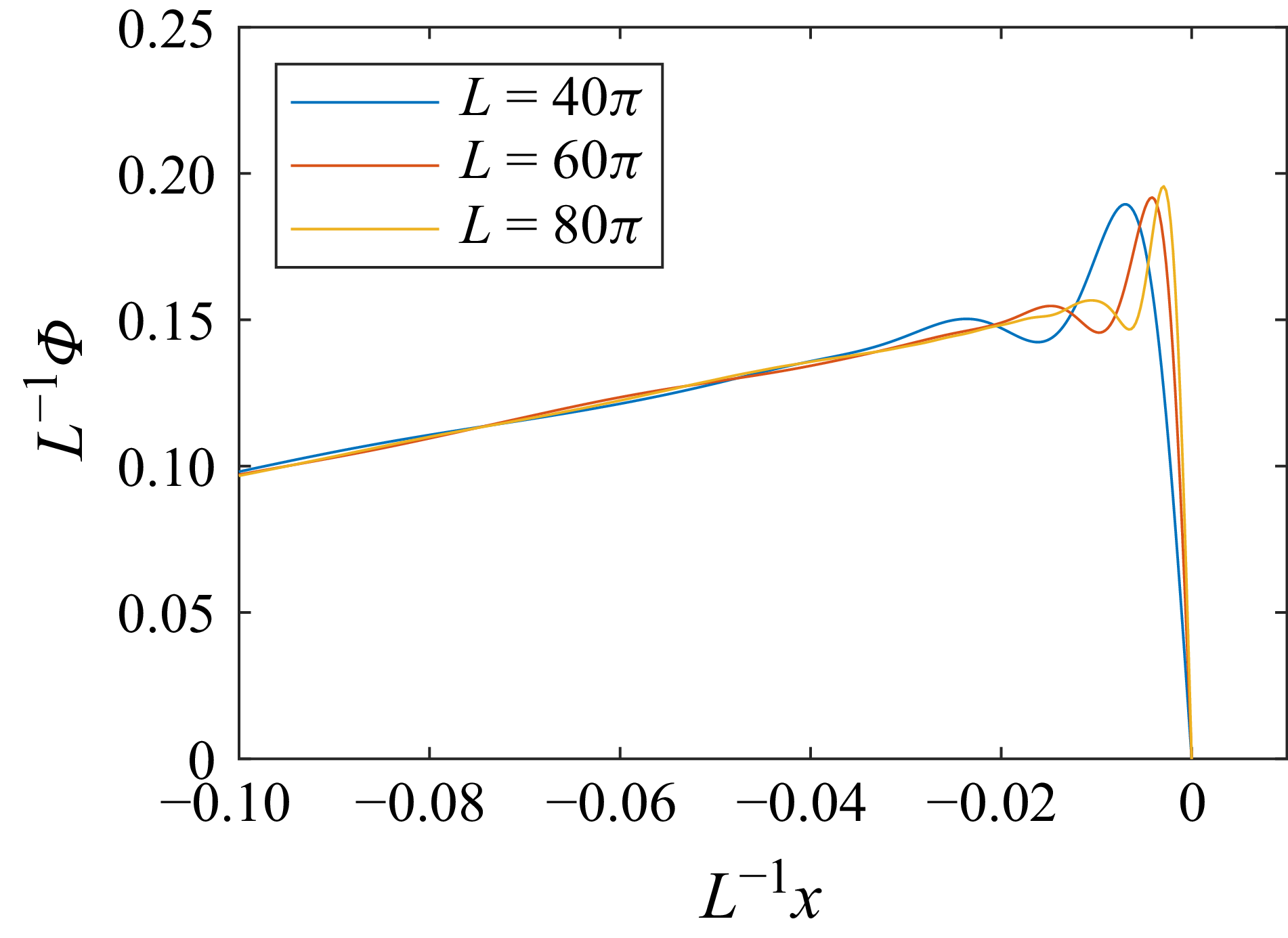
Nicolaenko, Scheurer & Temam (Reference Nicolaenko, Scheurer and Temam1985) estimated the size of the attractor using energy-type functions and derived an upper bound for the kinetic energy in the case of odd initial conditions. Subsequently, significant improvements in tightening this bound were achieved in multiple steps (Collet et al. Reference Collet, Eckmann, Epstein and Stubbe1993; Goodman Reference Goodman1994; Bronski & Gambill Reference Bronski and Gambill2006; Fantuzzi & Wynn Reference Fantuzzi and Wynn2015). Most of these studies construct analytic functions and rely on inequalities to bound the energy ball. An exception is the study by Fantuzzi & Wynn (Reference Fantuzzi and Wynn2015), in which the authors employed sum-of-squares techniques and semidefinite programming to optimise the energy ball estimates. They investigated how the radius scales with system parameters, thereby validating prior analytical predictions (Nicolaenko et al. Reference Nicolaenko, Scheurer and Temam1985; Bronski & Gambill Reference Bronski and Gambill2006). In these analyses, the velocity field is decomposed as
 $u(x,t) = v(x,t) + \varPhi (x)$
. The function
 $\varPhi (x)$
is constructed to bound the energy of
 $v$
, from which the corresponding estimate for
 $u$
is deduced.
A similar decomposition of the velocity field is referred to as the ‘background method’ in the case of the Navier–Stokes equations (Doering & Constantin Reference Doering and Constantin1992; Constantin & Doering Reference Constantin and Doering1995; Doering & Constantin Reference Doering and Constantin1996; Kerswell Reference Kerswell1998, Reference Kerswell1999; Fantuzzi, Arslan & Wynn Reference Fantuzzi, Arslan and Wynn2022; Chernyshenko Reference Chernyshenko2022). However, these studies focus on bounding time-averaged bulk quantities, such as momentum transport or the rate of viscous dissipation. Such analyses also require proving the existence of the energy ball, but its size is typically not calculated, with the exception of works such as Doering & Constantin (Reference Doering and Constantin1992), where the size of the absorbing ball is provided after their equation (20).
The background method has been applied to determine upper bounds on dissipation in canonical configurations such as plane Couette flow (PCF) (Plasting & Kerswell Reference Plasting and Kerswell2003), pipe flow (Plasting & Kerswell Reference Plasting and Kerswell2004), helical pipe flow (Kumar Reference Kumar2020), flow over a flat plate (Kumar & Garaud Reference Kumar and Garaud2020) and Taylor–Couette flow (Kumar Reference Kumar2022). However, a well-known limitation of this approach is that the mathematically rigorous bounds are often orders of magnitude larger than the values observed in physical turbulence. Furthermore, the optimal background fields that yield these bounds often bear little resemblance to observed mean velocity profiles. Recent advancements have sought to refine these methods, for instance, by employing sum-of-squares programming to construct non-quadratic Lyapunov functions (Chernyshenko et al. Reference Chernyshenko, Goulart, Huang and Papachristodoulou2014) or by applying the framework to more complex problems, such as determining bounds on the drag force on immersed bodies (Chernyshenko Reference Chernyshenko2025). A notable recent development in this area has shown that for three-dimensional planar shear flows, the optimisation problem for the dissipation bound can be rigorously reduced to a two-dimensional problem, significantly improving the tractability of the calculations (Rajkotia-Zaheer & Goluskin Reference Rajkotia-Zaheer and Goluskin2025).
The present work pursues a related but conceptually distinct objective within this framework. Instead of seeking bounds on a specific bulk quantity, the aim here is to identify the smallest possible ‘absorbing ball’ in the infinite-dimensional state space of the flow, analogous to the studies for the KS equation. To the best of the author’s knowledge, such an analysis has not been carried out for the infinite-dimensional Navier–Stokes equations.
The sketch of the minimal absorbing zone around the optimal background flow.

A schematic illustration of an absorbing ball is provided in figure 1. For shear flows, the existence of such a ball can be rigorously established using the Reynolds–Orr identity, which demonstrates that the nonlinear advection terms make no direct contribution to the evolution of the global kinetic energy of the fluctuations. It follows that this ball must contain all possible long-term attractors of the system, including the turbulent attractor.
Furthermore, these minimal energy balls may be utilised to improve the limit for the global stability of the laminar base flow. Global stability can be proved by the classical energy method (Reynolds–Orr equation) Orr (Reference Orr1907), but the predicted Reynolds number limit is usually one order of magnitude smaller than that observed in physical and numerical experiments.
Significant improvements have been made in this area utilising more complex energy functionals (Joseph & Tao Reference Joseph and Tao1963; Joseph Reference Joseph1978; Moffatt Reference Moffatt1990; Drazin & Reid Reference Drazin and Reid2004; Goulart & Chernyshenko Reference Goulart and Chernyshenko2012; Falsaperla et al. Reference Falsaperla, Giacobbe and Mulone2019, Reference Falsaperla, Mulone and Perrone2022; Nagy Reference Nagy2022; Fuentes, Goluskin & Chernyshenko Reference Fuentes, Goluskin and Chernyshenko2022; Nagy & Kulcsár Reference Nagy and Kulcsár2023), but the gap remains substantial. Here, an alternative approach is proposed. If the minimal absorbing ball lies within the provable region of attraction of the laminar state, then the laminar state is a global attractor.
An efficient way to construct a conditional Lyapunov function for the laminar flow was presented by Nagy (Reference Nagy2025), assuming a finite-dimensional dynamical system. This approach, combined with the infinite-dimensional framework of Goulart & Chernyshenko (Reference Goulart and Chernyshenko2012), can provide a provable region of attraction for the infinite-dimensional system. The key idea of this infinite-dimensional model is that the flow is described by a finite-dimensional system of ordinary differential equations, where the effect of truncation is not neglected but rigorously bounded by eigenvalue analysis.
In this paper, a gradient-based optimisation procedure is developed and implemented to minimise the absorbing ball for two canonical wall-bounded shear flows: PCF and plane Poiseuille flow (PPF).
The paper is organised as follows. Section 2 establishes the theoretical framework, while § 3 details the numerical solution method. Results are presented and discussed in § 4, followed by conclusions in § 5. Finally, Appendix A provides an analysis of the scaling law between the absorbing ball radius and the Reynolds number, and Appendix B demonstrates the application of the method to the KS equation.
2. Theory
The non-dimensional Navier–Stokes equations, written with the Einstein summation convention, are
 \begin{align} \frac {\partial {u}_{i}}{\partial t}&=-{u}_{j}\frac {\partial {u}_{i}}{\partial x_j}-\frac {\partial {p}}{\partial x_i}+\frac {1}{\textit{Re}}\frac {\partial ^2 {u}_i}{\partial x_j \partial x_j} +f_i, \end{align}
 \begin{align} \frac {\partial {u}_{i}}{\partial x_i}&=0, \end{align}
where
 $u_i$
and
 $p$
are the velocity and the pressure fields,
 $f_i$
is an arbitrary momentum source. Here
 $Re = L_0 U_0 / \nu$
is the Reynolds number based on the characteristic length
 $L_0$
, velocity
 $U_0$
and kinematic viscosity
 $\nu$
.
Throughout this study, the boundary conditions and momentum source are assumed to be time-independent. Accordingly, a stationary background flow
 $U_i$
is introduced which satisfies the prescribed boundary conditions, such that
 $u_i$
becomes the remaining time-dependent fluctuations around this background flow. This field is also referred to as the perturbation in this study. Such a decomposition resembles stability analysis, where
 $U_i$
usually denotes the base flow, which is time-independent and satisfies the governing equations. However, the background flow in this analysis does not necessarily satisfy the time-independent governing equations; it is merely a state-space point complying with the boundary conditions and the incompressibility constraint.
After the decomposition, the following equation can be obtained:
 \begin{equation} \frac {\partial {u}_{i}}{\partial t}=-{U}_{j}\frac {\partial {U}_{i}}{\partial x_j}-{U}_{j}\frac {\partial {u}_{i}}{\partial x_j}-{u}_{j}\frac {\partial {U}_{i}}{\partial x_j}-{u}_{j}\frac {\partial {u}_{i}}{\partial x_j}-\frac {\partial {p}}{\partial x_i}+\frac {1}{\textit{Re}}\frac {\partial ^2 {U}_i}{\partial x_j \partial x_j} + \frac {1}{\textit{Re}}\frac {\partial ^2 {u}_i}{\partial x_j \partial x_j} +f_i, \end{equation}
subject to the incompressibility constraint
 $({\partial u_i}/{\partial x_i})=0$
.
The non-dimensional kinetic energy of the fluctuations is defined as
 \begin{equation} e = \frac {1}{2}\int _{\mathcal{V}} {u}_{i}u_{i} \; \mathrm{d}\mathcal{V}{,} \end{equation}
where
 $\mathcal{V}$
denotes the flow domain. The derivative of kinetic energy with respect to time is
 \begin{equation} \frac {\mathrm{d}e}{\mathrm{d}t}= \int _{\mathcal{V}} \left ( -u_i {U}_{j}\frac {\partial {U}_{i}}{\partial x_j}-u_i{u}_{j}\frac {\partial {U}_{i}}{\partial x_j}+u_i\frac {1}{\textit{Re}}\frac {\partial ^2 {U}_i}{\partial x_j \partial x_j} + u_i\frac {1}{\textit{Re}}\frac {\partial ^2 {u}_i}{\partial x_j \partial x_j} + u_i f_i \right )\; \mathrm{d}\mathcal{V}{.} \end{equation}
Here, certain terms have been eliminated by applying the Gauss divergence theorem and assuming periodic, far-field vanishing or wall-bounded (no-slip wall condition) velocity fluctuations. These steps are analogous to those used in the proof of the well-known Reynolds–Orr identity (Reynolds Reference Reynolds1895; Orr Reference Orr1907; Schmid & S Henningson Reference Schmid and S Henningson2001). A significant consequence of this simplification is that the nonlinear terms (
 $u_j \partial u_i /\partial x_j$
) do not affect the time derivative of the kinetic energy. This observation is also a contributing factor to the Sommerfeld paradox (Sommerfeld Reference Sommerfeld and Castelnuovo1909; Li & Lin Reference Li and Lin2011; Falsaperla, Giacobbe & Mulone Reference Falsaperla, Giacobbe and Mulone2019). Furthermore, this simplification substantially facilitates the proof of the existence of an absorbing zone.
Such a zone attracts all of the trajectories, meaning that the flow state can be outside of the zone temporarily, as it evolves in time it will eventually enter the zone and be unable to escape. Consequently, the zone contains all possible attractors.
To prove the existence of such an absorbing zone, it is necessary to demonstrate that outside this zone, the kinetic energy decreases for any given state,
 \begin{equation} \frac {\mathrm{d}e}{\mathrm{d}t} \lt 0 \;\;\; \mathrm{if} \;\;\; e \gt e_{\textit{AZ}}[U_i], \end{equation}
where
 $e_{\textit{AZ}}[U_i]$
characterises the size of the absorbing ball, which depends on the background field. Usually, the smallest such ball is of interest. Let us temporarily fix the background field and define the largest possible time derivative among all possible perturbation fields (
 $u_i$
) as a function of the perturbation level (
 $\beta$
):
 \begin{equation} \dot {e}_{\textit{max}}(\beta ) = \max _{u_i} \left . \frac {\mathrm{d}e}{\mathrm{d}t} [u_i] \right |_{e=\beta }. \end{equation}
The requirement in (2.6) can be demonstrated by showing that
 \begin{equation} \lim _{\beta \to \infty } \dot {e}_{\textit{max}}(\beta ) \lt 0, \end{equation}
and
 \begin{equation} e_{\textit{AZ}} = \max \{ \beta \in \mathbb{R}_+ \mid \dot {e}_{\textit{max}}(\beta ) = 0 \}. \end{equation}
Geometrically, the maximal possible time derivative of energy on the surface of a ball characterised by
 $\beta$
around the background field is calculated. First, it must be demonstrated that this maximum is negative for an infinitely large ball. Then, the size of the ball is reduced to determine the largest possible
 $\beta$
for which this maximum (
 $\dot {e}_{\textit{max}}(\beta )$
) is zero on the surface of the ball. Consequently, outside this ball, the time derivative of the kinetic energy must be negative.
2.1. Infinite-amplitude perturbations
The maximum possible growth of kinetic energy associated with perturbations (fluctuations) of arbitrarily large amplitude about the background flow is examined first. In this limit, it is convenient to investigate the temporal growth rate of the kinetic energy defined as
 \begin{equation} \mu _e = \frac {1}{e}\frac {\mathrm{d}e}{\mathrm{d}t}. \end{equation}
It can be shown that, as the perturbation energy tends to infinity, the terms in (2.5) that scale linearly with
 $u_i$
vanish, yielding
 \begin{equation} \mu _e \to \mu _{e,\infty }= \frac {1}{e}\int _{\mathcal{V}}\left ( -u_i{u}_{j}\frac {\partial {U}_{i}}{\partial x_j}+ u_i\frac {1}{\textit{Re}}\frac {\partial ^2 {u}_i}{\partial x_j \partial x_j} \right ) \mathrm{d}\mathcal{V} \;\;\;\; \mathrm{as} \;\;\;\; e \to \infty . \end{equation}
For such states the growth rate is independent of the perturbation amplitude; consequently, the maximum achievable growth depends solely on the spatial structure of the velocity field.
The variation of the following Lagrangian is computed,
 \begin{equation} \mathcal{L}_{\mu _{e,\infty }} [u_i,q] = \frac {1}{e} \int _{\mathcal{V}} \left ( -u_i{u}_{j}\frac {\partial {U}_{i}}{\partial x_j} + \frac {u_i}{\textit{Re}}\frac {\partial ^2 {u}_i}{\partial x_j \partial x_j} + q \frac {\partial u_i}{\partial x_i} \right ) \, \mathrm{d}\mathcal{V}, \end{equation}
where the space-dependent field
 $q$
acts as a Lagrange multiplier field enforcing the divergence-free constraint on
 $u_i$
.
The maximum of
 $\mu _{e,\infty }$
is obtained by solving the associated Euler–Lagrange equations,
 \begin{equation} -u_j\left (\frac {\partial {U}_{i}}{\partial x_j}+\frac {\partial {U}_{j}}{\partial x_i}\right )+\frac {2}{\textit{Re}}\frac {\partial {}^2{u}_{i}}{\partial x_j\partial x_j}-\frac {\partial q}{\partial x_i} = \mu _{e,\infty } u_i. \end{equation}
Equations (2.13) and (2.2) form an eigenvalue problem in which
 $\mu _{e,\infty }$
is the eigenvalue. The largest eigenvalue represents the maximum possible growth rate, and the corresponding eigenfunction
 $\tilde {u}_i$
is referred to as the critical infinite perturbation. The first requirement for the existence of an absorbing zone, defined in (2.8), is fulfilled if this eigenvalue is negative, indicating that trajectories initialised sufficiently far from the background flow are attracted towards it. This is also known as the spectral constraint in the background method (Fantuzzi et al. Reference Fantuzzi, Arslan and Wynn2022; Kumar Reference Kumar2022).
As a trajectory approaches
 $U_i$
, its energy decreases; therefore, the linear terms neglected for large perturbations become significant, and the maximum possible growth rate increases.
2.2. Finite-amplitude perturbations
The critical energy level at which the maximal possible growth rate of the perturbation energy first becomes zero when the energy is decreased from infinity is now determined. This threshold defines the boundary of the absorbing zone. Outside this zone every trajectory must converge towards it because the growth rate is negative there. The radius of the absorbing ball is therefore obtained by evaluating the maximum of
 $\mathrm{d}e / \mathrm{d}t$
at successive energy levels while the energy is reduced and by identifying the critical level at which this maximum changes sign. The constrained maximum is determined by another Euler–Lagrange equation. The admissible velocity fields are required to be divergence-free and to possess a prescribed energy level
 $\beta$
:
 \begin{equation} \beta - \frac {1}{2}\int _{\mathcal{V}} {u}_{i}u_{i} \; \mathrm{d}\mathcal{V} = 0. \end{equation}
This constraint is enforced through the Lagrange multiplier
 $\mu _L$
, while the divergence-free condition is imposed by the field
 $q$
as in the previous subsection. Therefore, the Lagrangian in this case is given by
 \begin{align} \mathcal{L}_{\textit{d}e/\mathrm{d}t} &= \!\int _{\mathcal{V}} \!\left ( \!-u_i {U}_{j}\frac {\partial {U}_{i}}{\partial x_j}-u_i{u}_{j}\frac {\partial {U}_{i}}{\partial x_j}+u_i\frac {1}{\textit{Re}}\frac {\partial ^2 {U}_i}{\partial x_j \partial x_j} + u_i\frac {1}{\textit{Re}}\frac {\partial ^2 {u}_i}{\partial x_j \partial x_j} + u_i f_i+q \frac {\partial u_i}{\partial x_i} \!\right ) \mathrm{d} \mathcal{V} \nonumber \\&\quad + \mu _L \left ( \beta - \frac {1}{2}\int _{\mathcal{V}} {u}_{i}u_{i}\mathrm{d} \mathcal{V} \right )\!. \end{align}
The resulting Euler–Lagrange equations read
 \begin{equation} -u_j\left (\frac {\partial {U}_{i}}{\partial x_j}+\frac {\partial {U}_{j}}{\partial x_i}\right )+\frac {2}{\textit{Re}}\frac {\partial {}^2{u}_{i}}{\partial x_j\partial x_j}-\frac {\partial q}{\partial x_i} - \mu _L u_i =U_j \frac {\partial U_i}{\partial x_j} - \frac {1}{\textit{Re}}\frac {\partial {}^2{U}_{i}}{\partial x_j\partial x_j} - f_i {.} \end{equation}
Any extremum, such as
 $\dot {e}_{\textit{max}}$
, must satisfy this equation. Equations (2.2), (2.14) and (2.16) must be solved simultaneously to obtain candidate critical perturbations. The true critical state is the one whose energy
 $\beta$
is maximal and for which the time derivative of the kinetic energy vanishes (see (2.9)). Multiple solutions may exist for a given energy level because (2.14) is nonlinear.
2.2.1. Normal solutions
The eigenvalues
 $\mu _{e,\infty }$
obtained from (2.13) and (2.2) are also eigenvalues of the operator appearing on the left-hand side of the Euler–Lagrange equation (2.16) together with (2.2). If
 $\mu _L = \mu _{e,\infty }$
, the Euler–Lagrange equation becomes singular and must be handled separately. In figure 2, these eigenvalues are indicated by vertical dashed red lines, and the associated singularities are clearly visible. Otherwise, for practical implementation it is convenient to treat the Lagrange multiplier
 $\mu _L$
as a free parameter and to solve only the linear (2.2) and (2.16). The energy level
 $\beta$
then emerges as part of the solution instead of being prescribed a priori. Among the resulting states, the one satisfying
 $\mathrm{d}e/\mathrm{d}t = 0$
and yielding the largest
 $\beta$
is selected.
Time derivative of the kinetic energy (a,b) and energy level (c,d) of the normal solutions of (2.2), (2.14) and (2.16) as functions of the Lagrange multiplier
 $\mu _L$
. Solutions for which
 $\mathrm{d}e/\mathrm{d}t = 0$
are marked by purple crosses. Panels (b) and (d) provide zoomed views of panels (a) and (c), respectively, focusing on the neighbourhood of the critical value
 $\mu _L = -0.0352$
. The results correspond to PPF at
 $Re = 140$
with the background flow:
 $U_1 = (1-y^2)(-1.56y^6+1.8y^4+0.41y^2+0.7)$
.

Figure 2 illustrates this procedure by plotting the energy level of these solutions and the corresponding time derivative of the kinetic energy as functions of
 $\mu _L$
. In the example shown, three values of
 $\mu _L$
yield
 $\mathrm{d}e/\mathrm{d}t = 0$
among non-singular solutions. The largest energy level belongs to the largest
 $\mu _L$
among these values; and the associated fluctuation velocity field is termed the critical finite perturbation. The other two solutions correspond to local extrema only. In figure 3, the time derivative of the kinetic energy as a function of
 $\beta$
is plotted for the same solutions. The global maximum of these solutions (
 $\dot {e}_{\textit{max}}(\beta )$
) is plotted as a continuous blue curve, while the other extrema appear as a dashed curve. The three normal solutions of the Euler–Lagrange equation, for which
 $\mathrm{d}e/\mathrm{d}t$
is 0, are clearly visible. However, a singular solution may result in an even larger critical energy level, so it must also be considered to determine the true size of the absorbing ball.
The maximum of the time derivative of kinetic energy,
 $\dot {e}_{\textit{max}}(\beta )$
. The parameters are the same as in figure 2. The blue curves are the normal solutions of (2.2), (2.14), and (2.16). Continuous blue line represents the true maximum among normal solutions, while the dashed curves represent other extremums. The orange dash–dotted ray represents the singular solutions. The critical normal solutions are denoted by purple crosses, the critical singular solution is denoted with an orange cross.

2.2.2. Singular solutions
If
 $\mu _L = \mu _{e,\infty }$
, the linear operator on the left-hand side of the Euler–Lagrange equation (2.16) becomes singular. Analytically, according to the Fredholm alternative, a bounded exact solution to this system exists if the load vector on the right-hand side is orthogonal to the critical eigenvector
 $\tilde {u}_i$
:
 \begin{equation} \int _{\mathcal{V}} \tilde {u}_i \left (U_j \frac {\partial U_i}{\partial x_j} - \frac {1}{\textit{Re}}\frac {\partial {}^2{U}_{i}}{\partial x_j\partial x_j} - f_i\right ) \mathrm{d}\mathcal{V} = 0. \end{equation}
When this condition is met, a family of resonance solutions emerges, taking the form
 \begin{equation} u_{\textit{s},i} = u_{\textit{p},i} + a \tilde {u}_i, \end{equation}
where
 $u_{\textit{p},i}$
is a particular solution of (2.2) and (2.16), and
 $a$
is an arbitrary scalar representing the amplitude of the eigenvector.
In a practical numerical framework, computing solutions at or very close to
 $\mu _L = \mu _{e,\infty }$
requires special treatment because standard linear solvers fail when the operator is singular or highly ill-conditioned. To resolve this, the pseudoinverse can be employed to compute the particular solution
 $u_{\textit{p},i}$
. Furthermore, while the strict orthogonality condition (2.17) holds naturally in certain cases – such as for specific wave-like eigenvectors – it is not always satisfied exactly due to general background flow configurations or discretisation errors. If one simply approached the singularity without exact orthogonality, the numerical solution would become strongly dominated by the eigenvector
 $\tilde {u}_i$
, with an amplitude scaling as
 $1/(\mu _L - \mu _{e,\infty })$
. By using the pseudoinverse, the system is solved in a least-squares sense. This not only natively handles the singular operator to yield the minimum-norm particular solution, but it also automatically projects the load vector onto the column space of the operator, effectively filtering out any problematic non-orthogonal components.
The time derivative of the kinetic energy for these solutions is
 \begin{equation} \frac {\mathrm{d}e}{\mathrm{d}t}\big[u_{\textit{s},i} \big] = \frac {\mathrm{d}e}{\mathrm{d}t}\big[u_{\textit{p},i}\big] + a^2 \frac {\mathrm{d}e}{\mathrm{d}t}\big[\tilde {u}_i\big]. \end{equation}
If the eigenvector is normalised such that
 $e[\tilde {u}_i]=1$
, then the expression can be rewritten as
 \begin{equation} \frac {\mathrm{d}e}{\mathrm{d}t}\big[u_{\textit{s},i} \big] = \frac {\mathrm{d}e}{\mathrm{d}t}\big[u_{\textit{p},i}\big] + a^2 \mu _{e,\infty }. \end{equation}
Therefore, these solutions form a ray if
 $\dot {e}_{\textit{max}}$
is plotted as a function of
 $\beta$
with a slope
 $\mu _{e,\infty }$
, resulting in a side branch from the normal solutions; see figure 3, where the dash–dotted orange line represents these solutions. If
 $\dot {e}[u_{\textit{p},i}] \gt 0$
and
 $\mu _{e,\infty } \lt 0$
, then there are two critical solutions where
 $\dot {e}[u_{\textit{s},i}] = 0$
:
 \begin{equation} a = \pm \sqrt {-\frac {1}{\mu _{e,\infty }} \frac {\mathrm{d}e}{\mathrm{d}t}\big[u_{\textit{p},i}\big]}. \end{equation}
Both solutions result in the same critical energy level,
 \begin{equation} e_{\textit{AZ, s}} = e\big[u_{\textit{p},i}\big] + a^2 = e\big[u_{\textit{p},i}\big] - \frac {1}{\mu _{e,\infty }} \frac {\mathrm{d}e}{\mathrm{d}t}\big[u_{\textit{p},i}\big] . \end{equation}
If this energy level is larger than the critical energy level among normal solutions, this will be the true critical one, and it determines the size of the absorbing ball. It should be noted that such a resonant solution can exist for any eigenvalue, but the critical state corresponds to the largest eigenvalue.
The procedure for computing the absorbing zone around a given background flow
 $U_i$
is summarised as follows:
-
(i) solve (2.13) and (2.2) to obtain the largest eigenvalue
 $\mu _{e,\infty }$
; if
$\mu _{e,\infty } \gt 0$
, the absorbing zone does not exist, otherwise, continue with the following steps;
-
(ii) investigate the normal solutions and solve (2.16) and (2.2) for various values of
$\mu _L$
and adjust
$\mu _L$
until
$\mathrm{d}e / \mathrm{d}t = 0$
meaning that(2.23)
\begin{equation} \int _{\mathcal{V}}\!\left ( -u_i U_j\frac {\partial U_i}{\partial x_j} -u_i u_j\frac {\partial U_i}{\partial x_j} +\frac {1}{\textit{Re}}\,u_i\frac {\partial ^2 U_i}{\partial x_j\partial x_j} +\frac {1}{\textit{Re}}\,u_i\frac {\partial ^2 u_i}{\partial x_j\partial x_j} +u_i f_i \right )\,\mathrm{d}\mathcal{V} \;=\; 0 ; \end{equation}
-
(iii) among the (possibly several) solutions that satisfy (2.23), select the one with the highest energy, this energy is denoted by
$e_{\textit{AZ, n}}$
; -
(iv) investigate the singular solutions corresponding to the largest eigenvalue
$\mu _{e,\infty }$
; iIf
$\dot {e}[u_{\textit{part},i}] \gt 0$
, determine
$e_{\textit{AZ, s}}$
utilising (2.21) and (2.22); -
(v) select the largest critical perturbation level,
$e_{\textit{AZ}} = \max (e_{\textit{AZ, n}}, e_{\textit{AZ, s}})$
.


2.3. Minimising the absorbing zone
For a given flow configuration several admissible background flows
 $U_i$
may exist, each of which possesses its own absorbing zone. In general, the background flow that generates the smallest absorbing zone must be selected. The selection can be formulated as the optimisation problem
 \begin{equation} e_{\textit{AZ, opt}} = \min _{U_i} e_{\textit{AZ}} [U_i] {.} \end{equation}
The functional derivative of
 $e_{\textit{AZ}}$
with respect to
 $U_i$
depends on whether the critical state belongs to a normal or singular solution. In both cases, the functional derivative requires the inversion of an operator; therefore, it cannot be written in explicit form, and the corresponding Euler–Lagrange equation is not solved directly. Instead, the direct optimisation of
 $e_{\textit{AZ}}$
is proposed using gradient-based methods similar to, for example, minimal seed calculations (Pringle, Willis & Kerswell Reference Pringle, Willis and Kerswell2012; Kerswell, Pringle & Willis Reference Kerswell, Pringle and Willis2014; Cherubini, De Palma & Robinet Reference Cherubini, De Palma and Robinet2015).
2.3.1. Sensitivity in the case of normal solutions
The computational time of the optimisation can be reduced by deriving an analytic expression for the sensitivity of
 $e_{\textit{AZ}}$
to variations in the background flow. When the critical state corresponds to a normal solution, this leads to
 \begin{equation} \frac {\delta e_{\textit{AZ,n}}}{\delta U_i} = u_j \frac {\delta u_j}{\delta U_i} {,} \end{equation}
where
 $({\delta u_j}/{\delta U_i})$
is the sensitivity of the critical finite perturbation with respect to modifications of the background flow. It is obtained by perturbing (2.16), (2.2) and (2.23) leading to the following equation system:
 \begin{align} &\begin{bmatrix} A_{11} & -\left (\frac {\partial U_1}{\partial x_2} +\frac {\partial U_2}{\partial x_1} \right ) & -\left (\frac {\partial U_1}{\partial x_3} +\frac {\partial U_3}{\partial x_1} \right )& -\frac {\partial }{\partial x_1}& -u_1 \\[10pt] -\left (\frac {\partial U_2}{\partial x_1} +\frac {\partial U_1}{\partial x_2} \right ) &A_{22} & -\left (\frac {\partial U_2}{\partial x_3} +\frac {\partial U_3}{\partial x_2} \right )& -\frac {\partial }{\partial x_2}& -u_2 \\[10pt] -\left (\frac {\partial U_3}{\partial x_1} +\frac {\partial U_1}{\partial x_3} \right ) & -\left (\frac {\partial U_3}{\partial x_2} +\frac {\partial U_2}{\partial x_3} \right )&A_{33} & -\frac {\partial }{\partial x_3}& -u_3 \\[10pt] \frac {\partial }{\partial x_1}& \frac {\partial }{\partial x_2}&\frac {\partial }{\partial x_3} & 0 & 0\\[10pt] A_{51}& A_{52}&A_{53} & 0 & 0 \end{bmatrix} \begin{bmatrix} \delta u_1 \vphantom {\left (\frac {\partial U_1}{\partial x_2}\right )} \\ \delta u_2 \vphantom {\left (\frac {\partial U_1}{\partial x_2}\right )} \\ \delta u_3 \vphantom {\left (\frac {\partial U_1}{\partial x_2}\right )} \\ \delta q \vphantom {\frac {1}{1}}\\ \delta \mu _L \end{bmatrix} \notag\\[10pt] &\quad = \begin{bmatrix} B_{11} & u_2\frac {\partial }{\partial x1} + \frac {\partial U_1}{\partial x_2} & u_3\frac {\partial }{\partial x_1} + \frac {\partial U_1}{\partial x_3} \\[10pt] u_1\frac {\partial }{\partial x_2} + \frac {\partial U_2}{\partial x_1} & B_{22} & u_3\frac {\partial }{\partial x_2} + \frac {\partial U_2}{\partial x_3} \\[10pt] u_1\frac {\partial }{\partial x_3} + \frac {\partial U_3}{\partial x_1} & u_2\frac {\partial }{\partial x_3} + \frac {\partial U_3}{\partial x_2}& B_{33} \\[10pt] 0 &0 &0 \\ B_{51} &B_{52} &B_{53} \end{bmatrix} \begin{bmatrix} \delta U_1 \vphantom {\left (\frac {\partial U_1}{\partial x_2}\right )} \\ \delta U_2 \vphantom {\left (\frac {\partial U_1}{\partial x_2}\right )} \\ \delta U_3 \vphantom {\left (\frac {\partial U_1}{\partial x_2}\right )} \end{bmatrix}. \end{align}
The operators appearing above are defined by
 \begin{align} T_{ij} &= \frac {\partial U_i}{\partial x_j} {,} \end{align}
 \begin{align} A_{ii} &= -2 T_{ii} + \frac {2}{\textit{Re}} \frac {\partial ^2}{\partial x_j \partial x_j} - \mu _L, \end{align}
 \begin{align} A_{5i} &= -{U}_{j}\frac {\partial {U}_{i}}{\partial x_j}-{u}_{j}\left (\frac {\partial {U}_{i}}{\partial x_j} +\frac {\partial {U}_{j}}{\partial x_i} \right )+\frac {1}{\textit{Re}}\frac {\partial ^2 {U}_i}{\partial x_j \partial x_j} + \frac {2}{\textit{Re}}\frac {\partial ^2 {u}_i}{\partial x_j \partial x_j} + f_i {,} \end{align}
 \begin{align} B_{\textit{11}} &= u_j \frac {\partial }{\partial x_j} + u_1 \frac {\partial }{\partial x_1} + \frac {\partial U_1}{\partial x_1} + U_j \frac {\partial }{\partial x_j} -\frac {1}{\textit{Re}} \frac {\partial ^2 }{\partial x_j \partial x_j}{,} \end{align}
 \begin{align} B_{\textit{22}} &= u_j \frac {\partial }{\partial x_j} + u_2 \frac {\partial }{\partial x_2} + \frac {\partial U_2}{\partial x_2} + U_j \frac {\partial }{\partial x_j} -\frac {1}{\textit{Re}} \frac {\partial ^2 }{\partial x_j \partial x_j} {,} \end{align}
 \begin{align} B_{\textit{33}} &= u_j \frac {\partial }{\partial x_j} + u_3 \frac {\partial }{\partial x_3} + \frac {\partial U_3}{\partial x_3} + U_j \frac {\partial }{\partial x_j} -\frac {1}{\textit{Re}} \frac {\partial ^2 }{\partial x_j \partial x_j} {,} \end{align}
 \begin{align} B_{5i} &= {u}_{j}\frac {\partial {U}_{j}}{\partial x_i}-{U}_{j}\frac {\partial {u}_{i}}{\partial x_j} -{u}_{j}\frac {\partial {u}_{i}}{\partial x_j} -\frac {1}{\textit{Re}}\frac {\partial ^2 u_i}{\partial x_j \partial x_j} . \end{align}
Calculating
 ${\delta u_j}/{\delta U_i}$
requires inverting the operator on the left-hand side of (2.26), a task that is computationally unfeasible in most cases. However, this difficulty can be overcome by directly evaluating (2.25), where the computation can be rearranged as solving a linear equation. After discretisation of the problem, the sensitivity (2.25) can be calculated as
 \begin{equation} \boldsymbol{s}_{e,U_i} = \big(\boldsymbol{v} \boldsymbol{A}^{-1}\big) \boldsymbol{B}, \end{equation}
where
 $\boldsymbol{v} = [\boldsymbol{u}^T, \boldsymbol{0}^T, 0]$
,
 $\boldsymbol{u}^T$
is the discretised critical velocity field solution of ((2.2), (2.14), (2.16)),
 $\boldsymbol{0}$
is a zero vector of length equal to that of the discretised
 $q$
field, and
 $\boldsymbol{A}$
and
 $\boldsymbol{B}$
are the discretised operators on the left- and right-hand sides of (2.26), including the boundary conditions. Rather than directly inverting
 $\boldsymbol{A}$
, a vector
 $\boldsymbol{\lambda }^T = \boldsymbol{v} \boldsymbol{A}^{-1}$
can be defined, and the transposed system
 $\boldsymbol{A}^T \boldsymbol{\lambda } = \boldsymbol{v}^T$
can be solved. The sensitivity can be then efficiently recovered through a single matrix–vector product,
 $\boldsymbol{\lambda }^T \boldsymbol{B}$
. Mathematically, this algebraic rearrangement is identical to a discrete adjoint approach.
2.3.2. Sensitivity in the case of singular solutions
When the critical state corresponds to a singular solution, the size of the absorbing zone is determined by (2.22). To optimise the background flow, the total sensitivity of this quantity is required with respect to variations in
 $U_i$
. Applying the chain rule yields three distinct contributions,
 \begin{equation} \frac {\delta e_{\textit{AZ,s}}}{\delta U_i} = \frac {\delta e_{\textit{p}}}{\delta U_i} - \frac {1}{\mu _{e,\infty }}\frac {\delta \dot {e}_{\textit{p}}}{\delta U_i} + \frac {\dot {e}_{\textit{p}}}{\mu _{e,\infty }^2}\frac {\delta \mu _{e,\infty }}{\delta U_i}, \end{equation}
where
 $e_{\textit{p}} = e[u_{\textit{p},i}]$
and
 $\dot {e}_{\textit{p}} = \dot {e}_{\textit{p}} [u_{\textit{p},i}]$
. This leads to
 \begin{equation} \frac {\delta e_{\textit{AZ,s}}}{\delta U_i} = \frac {\partial e_{\textit{p}}}{\partial u_{\textit{p},j}}\frac {\delta u_{\textit{p},j}}{\delta U_i} - \frac {1}{\mu _{e,\infty }} \left (\frac {\partial \dot {e}_{\textit{p}}}{\partial u_{\textit{p},j}} \frac {\delta u_{\textit{p},j}}{\delta U_i} + \frac {\partial \dot {e}_{\textit{p}}}{\partial U_i}\right ) + \frac {\dot {e}_{\textit{p}}}{\mu _{e,\infty }^2}\frac {\delta \mu _{e,\infty }}{\delta U_i}. \end{equation}
The terms can be rearranged as
 \begin{equation} \frac {\delta e_{\textit{AZ,s}}}{\delta U_i} = \underbrace {\left ( \frac {\partial e_{\textit{p}}}{\partial u_{\textit{p},j}} - \frac {1}{\mu _{e,\infty }}\frac {\partial \dot {e}_{\textit{p}}}{\partial u_{\textit{p},j}} \right )}_{0} \frac {\delta u_{\textit{p},j}}{\delta U_i} - \frac {1}{\mu _{e,\infty }} \frac {\partial \dot {e}_{\textit{p}}}{\partial U_i} + \frac {\dot {e}_{\textit{p}}}{\mu _{e,\infty }^2}\frac {\delta \mu _{e,\infty }}{\delta U_i} , \end{equation}
where the first term is zero because the expression in the brackets satisfies (2.16), noting that for singular solutions
 $\mu _L = \mu _{e,\infty }$
. The remaining terms are as follows:
 \begin{equation} \frac {\partial \dot {e}_{\textit{p}}}{\partial U_i} = -u_{\textit{p},j}\frac {\partial {U}_{j}}{\partial x_i}+{U}_{j}\frac {\partial u_{\textit{p},i}}{\partial x_j} +u_{\textit{p},j}\frac {\partial u_{\textit{p},i}}{\partial x_j} +\frac {1}{\textit{Re}}\frac {\partial ^2 u_{\textit{p},i}}{\partial x_j \partial x_j}. \end{equation}
The last term, the sensitivity of the leading eigenvalue of the problem (2.13) with respect to the background field, is
 \begin{equation} \frac {\delta \mu _{e,\infty }}{\delta U_i} = 2 \tilde {u}_j \frac {\partial \tilde {u}_i}{\partial x_j} {,} \end{equation}
where
 $\tilde {u}_i$
is the eigenvector associated with the largest eigenvalue, namely the critical infinite perturbation. The fact that the eigenvectors are real-valued – owing to the symmetry of the linear operator in the eigenvalue problem (2.13) and (2.2) – was invoked in the derivation of this expression. A similar eigenvalue sensitivity analysis was utilised by Bottaro, Corbett & Luchini (Reference Bottaro, Corbett and Luchini2003) to investigate the effect of base-flow variations on standard linear stability instead of energy stability. However, a further key distinction is that while Bottaro et al. (Reference Bottaro, Corbett and Luchini2003) constrained the variation using an energy-like norm on the base flow, the present energy stability framework instead fixes the energy of the perturbation. Expression (2.39) can also be utilised for efficient initialisation of the background field to satisfy the constraint
 $\mu _{e,\infty }\lt 0$
.
Using these gradients, the background flow can be optimised to minimise the absorbing zone.
3. Solution method for one-dimensional background flow
The optimisation procedure is first applied to PCF and PPF, where the base and optimal background flows reduce to one-dimensional wall-normal profiles but the perturbation fields
 $u_i$
remain three-dimensional. Throughout,
 $x_1$
,
 $x_2$
and
 $x_3$
denote the streamwise, wall-normal and spanwise coordinates, respectively; the background flows therefore depend solely on
 $x_2$
.
In this case, the eigenvalue problem, (2.2) and (2.13) can be simplified by assuming a complex waveform solution
 \begin{align} u_i\big(x_1, x_2, x_3\big) &= \hat {u}_i (x_2) \mathrm{e}^{ \mathrm{i}\left (k_1 x_1 + k_3 x_3\right ) } {,} \end{align}
 \begin{align} p \big(x_1, x_2, x_3\big) &= \hat {p} (x_2) \mathrm{e}^{\mathrm{i}\left (k_1 x_1 + k_3 x_3\right )} , \end{align}
with streamwise and spanwise wavenumbers
 $k_1$
and
 $k_3$
.
The substitution into (2.2) and (2.13) yields
 \begin{equation} \left [ \begin{array}{cccc} \frac {2}{\textit{Re}} \, L & -\frac {\mathrm{d}U_1}{\mathrm{d}x_2} & 0 & -\mathrm{i} k_1 \\[9pt] -\frac {\mathrm{d}U_1}{\mathrm{d}x_2} & \frac {2}{\textit{Re}}\,L & 0 & -D \\ 0 & 0 & \frac {2}{\textit{Re}}\, L & -\mathrm{i} k_3 \\[6pt] \mathrm{i} k_1 & D & \mathrm{i}k_3 & 0 \\ \end{array} \right ] \left [ \begin{array}{c} \hat {u}_1\\\hat {u}_2\\\hat {u}_3\\{\hat {q}_m} \end{array} \right ] = \tilde {\mu }_{e,\infty } \left [ \begin{array}{cccc} I & 0 & 0 & 0 \\ 0 & I & 0 & 0 \\ 0 & 0 & I & 0 \\ 0 & 0 & 0 & 0 \\ \end{array} \right ] \left [ \begin{array}{c} \hat {u}_1\\\hat {u}_2\\\hat {u}_3\\{\hat {q}_m} \end{array} \right ]{,} \end{equation}
where
 $L=D^2-(k_1^2+k_3^2)$
is the Laplace operator and
 $D = ({\mathrm{d}\square }/{\mathrm{d}x_2})$
is the differential operator with respect to
 $x_2$
,
 $I$
is the identity operator.
The true critical eigenvalue,
 ${\mu }_{e,\infty }$
is the largest one among all possible wavenumber pairs,
 \begin{equation} {\mu }_{e,\infty } = \max _{k_1, k_3} \tilde {\mu }_{e,\infty }. \end{equation}
The maximum is consistently found to occur at
 $k_1=0$
. This finding is analogous to the behaviour of the laminar base flow profile in PCF, as proven by Busse (Reference Busse1972).
The equation (2.16), the condition for maximal growth in the case of finite normal perturbations, simplifies similarly. It is also a linear equation; therefore, the complex Fourier transformation can be applied. Because the right-hand side contains only non-oscillatory terms
 $(k_1=k_3=0)$
, the left-hand side forces all oscillatory
 $\hat {u}_i$
to vanish, meaning that the critical finite normal perturbation field depends only on
 $x_2$
. The continuity equation then implies
 $u_2=u_3=0$
, so that
 \begin{equation} \frac {2}{\textit{Re}} \frac {\partial ^2 {u}_1}{\partial x_2 \partial x_2} - \mu _L u_1 = - \frac {1}{\textit{Re}}\frac {\partial {}^2{U}_{1}}{\partial x_2\partial x_2} - f_1 {.} \end{equation}
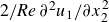
The operator (
 ${2}/{\textit{Re}} \; \partial ^2 {u}_1 /{\partial x_2^2}$
) on the left-hand side represents pure dissipation and is independent of the background flow. Assuming wall boundary conditions, its eigenvalues can be calculated analytically as
 $-j^2\pi ^2/(2\,Re)$
, where
 $j$
is an arbitrary positive integer. Equation (3.5) becomes singular only if
 $\mu _L$
equals one of these eigenvalues. In figure 2, only these specific singularities are visible. However, while these singular values correspond strictly to the zero-wavenumber limit, the full problem can exhibit singularities – with Fredholm alternative solutions – at other
 $\mu _L$
values for any other wavenumber pair. Among the eigenvalues in the zero-wavenumber limit, the largest (
 $j=1$
) is
 \begin{equation} \mu _d = -\frac {\pi ^2}{2\,\textit{Re}}. \end{equation}
Furthermore, as
 $k_1\to 0$
and
 $k_3\to 0$
, the eigenvalue problem (3.3) for
 $\tilde {\mu }_{e,\infty }$
reduces to this same dissipative operator (
 ${2}/{\textit{Re}} \; \partial ^2 {u}_1 /{\partial x_2^2}$
). Because the eigenvalues for this specific wavenumber pair are independent of the background flow,
 $\mu _d$
serves as a lower bound for
 ${\mu }_{e,\infty }$
for any flow configuration within this domain,
 \begin{equation} {\mu }_{e,\infty }\geqslant \mu _d. \end{equation}
The (2.26), which expresses the sensitivity, also reduces in one dimension to
 \begin{equation} \begin{bmatrix} \frac {2}{\textit{Re}}\,D^2 - \mu _L & -u_1 \\[8pt] \frac {1}{\textit{Re}} \left (D^2 U_1\, +\, 2 \, D^2 u_1 \right ) + f_1 & 0 \end{bmatrix} \begin{bmatrix} \delta u_1 \\ \delta \mu _L \end{bmatrix} = \begin{bmatrix} -\frac {1}{\textit{Re}}D^2 \\[10pt] -\frac {1}{\textit{Re}} D^2 u_1 \end{bmatrix} \begin{bmatrix} \delta U_1 \end{bmatrix}. \end{equation}
In the case of singular solutions, the particular part
 $u_{\textit{p}, i}$
has only a streamwise component and depends on
 $x_2$
, following the previous discussion. Meanwhile, the eigenvector that, when combined with the particular solution, maximises
 $\dot {e}$
at a given perturbation level corresponds to the largest eigenvalue,
 ${\mu }_{e,\infty }$
. Because this eigenfunction can take the form of a spanwise-oscillating three-dimensional wave, their superposition can also result in a fully three-dimensional field. Additionally, the one-dimensional particular solution allows (2.38) to be significantly reduced during sensitivity calculations,
 \begin{equation} \frac {\partial \dot {e}_{\textit{p}}}{\partial U_i} = -u_{\textit{p},j}\frac {\partial {U}_{j}}{\partial x_i}+{U}_{j}\frac {\partial u_{\textit{p},i}}{\partial x_j} +u_{\textit{p},j}\frac {\partial u_{\textit{p},i}}{\partial x_j} +\frac {1}{\textit{Re}}\frac {\partial ^2 u_{\textit{p},i}}{\partial x_j \partial x_j}. \end{equation}
When the background flow coincides with the laminar base flow, the terms in the momentum equation
 $(-{U}_{j}({\partial {U}_{i}}/{\partial x_j}) +( {1}/{\textit{Re}})({\partial ^2 {U}_i}/({\partial x_j \partial x_j})) + f_i)$
balance each other; therefore, the right-hand sides of (2.16) and (3.5) vanishes; consequently, the left-hand side must also be zero. Thus, the velocity field of both the normal solutions and the particular part of the singular solutions is zero. Therefore, only the singular solutions of the form
 $a\tilde {u}_i$
determine the possible maximum of the time derivative of the kinetic energy:
 $a^2 \mu _{e,\infty }$
. If
 $\mu _{e,\infty }\lt 0$
, then the maximum is zero everywhere except at
 $\beta =0$
; therefore, an absorbing zone exists with zero radius. The condition
 $\mu _{e,\infty }\lt 0$
holds whenever the Reynolds number lies below the global stability limit obtained from the classical Reynolds–Orr energy method,
 $Re\lt {\textit{Re}}_E$
. In that regime, the minimal absorbing zone collapses to a single point – the laminar base flow state – which is consistent with the base flow being a global attractor there.
Two configurations are examined: (i) PCF between moving walls, and (ii) PPF driven by a constant pressure gradient between stationary walls.
The Reynolds number is defined as
 \begin{equation}{\textit{Re}}= \frac {U_0 h }{\nu }{,} \end{equation}
where
 $h$
is the half-gap. For PCF
 $U_0$
is half the wall-speed difference; for PPF it is the centreline velocity of the laminar base flow. The forcing term
 $f_1$
vanishes for PCF and is chosen to yield the prescribed
 ${\textit{Re}}$
for PPF.
In the numerical study,
 ${\textit{Re}}$
was varied from
 $30$
to
 $800$
in increments of
 $10$
for PCF, and from
 $100$
to
 $5000$
in increments of
 $10$
for PPF. At each step the optimiser is initialised with the previously converged solution. In the first step, the laminar base flow was used, however, in the case of PCF a minor perturbation was necessary. Optimisation was carried out in MATLAB 2024b using the built-in fmincon routine with the interior-point algorithm. Spectral-collocation grids containing
 $65$
,
 $80$
and
 $90$
points were tested and produced indistinguishable results; the data presented below correspond to the
 $80$
-point grid.
4. Results
The dependence of the minimal absorbing zone on the Reynolds number is examined first. Although these solutions are referred to as minimal, due to the optimisation problem being non-convex, multiple local minima may exist, and it is not guaranteed that the presented result corresponds to the global minimum. Figure 4 displays the kinetic energy of the critical finite perturbation normalised by the kinetic energy of the laminar base flow. Below the classical energy-stability limits,
 ${\textit{Re}}_E=20.6625$
for PCF and
 ${\textit{Re}}_E=49.6035$
for PPF, the size of the region is zero. Immediately above these thresholds the zone expands rapidly, after which its growth reduces to an approximately linear trend in both configurations.
The observed linear scaling of the absorbing zone size,
 $e_{\textit{AZ}} \sim O({\textit{Re}})$
, is consistent with asymptotic estimates derived using the background method (Doering & Constantin Reference Doering and Constantin1992). The detailed derivation is given in Appendix A.
Even at modest Reynolds numbers the energy of the critical finite perturbation remains comparable to that of the base flow. For PPF the ratio stays below unity and grows only slowly, whereas in PCF it exceeds unity for
 $Re\gtrsim 130$
and increases more steeply.
Kinetic energy of the critical finite perturbation, normalised by the kinetic energy of the laminar base flow, for (a) PCF and (b) PPF.

The optimal background flow profiles and their corresponding critical finite perturbations are depicted in figure 5. For PCF, the velocity gradient near the wall increases sharply while the slope near the channel centre approaches zero. This behaviour reflects the requirement that, at high perturbation amplitudes, due to the spectral constraint the kinetic energy must decrease therefore viscous dissipation must dominate production. Since production is proportional to the product of fluctuation velocity and background flow shear, the shear is concentrated where the fluctuations must vanish due to boundary condition: close to the walls. Such near-wall localisation of the shear is a generic outcome of background method optimisations and is discussed in detail by Chernyshenko (Reference Chernyshenko2025).
In PPF the wall gradient grows only moderately, whereas the bulk velocity is markedly reduced. This is a consequence of the chosen non-dimensionalisation; a Reynolds number based on bulk velocity would reveal a more Couette-like trend.
The critical finite perturbation in both flow configurations changes little in shape as
 ${\textit{Re}}$
increases – only its amplitude grows.
Optimal background flow profiles (a,c) and their corresponding critical finite perturbations (normal solution or the particular part of singular solution) (b,d). Here PCF (a,b); PPF (c,d).

Eigenvalues corresponding to infinite-amplitude perturbations (a,b) and their associated critical spanwise wavenumbers,
 $k_3$
(c,d), for optimal background flow profiles. Results are shown for PCF (a,c) and PPF (b,d).

The largest eigenvalue (
 $\tilde {\mu }_{e,\infty }$
) of (3.3) as a function of the spanwise wavenumber (
 $k_3$
) for optimal background profiles at
 $Re = 200$
and
 $k_1=0$
.

The results are also compared with recent direct numerical simulations (DNS) from the literature (Cavalieri & Nogueira Reference Cavalieri and Nogueira2022) at
 $Re = 500$
for PCF, as shown in figure 5(a
). The turbulent mean profile is significantly less sharp close to the wall and does not satisfy the condition
 $\mu _{e,\infty } \lt 0$
. A positive eigenvalue does not imply that the turbulent mean is not attracting, but rather that it is easy to construct a perturbation field for it whose energy increases initially, resembling a transient growth mechanism.
The critical growth rate of the infinite amplitude perturbation,
 $\mu _{e,\infty }$
, as a function of the Reynolds number for optimal background flows is shown in figures 6(a) and 6(b). It can be clearly seen that after a short transient, the value tends towards the theoretical lower limit,
 $\mu _d$
, in the case of PCF. This is reasonable, since any sharper velocity profile increases the load of (3.5), which in turn increases the magnitude of the particular solution. Meanwhile,
 $\mu _{e,\infty }$
– which is also the slope of
 $\dot {e}$
as a function of the perturbation amplitude for a resonant solution (2.20) – cannot be further reduced; therefore, the size of the absorbing zone (where
 $\dot {e}_{\max } = 0$
) would increase. For PPF, the growth rate lies between the theoretical minimum,
 $\mu _d$
, and
 $0.5\mu _d$
, and after a longer transient, it tends towards
 $0.5\mu _d$
. This behaviour can be explained by that the magnitude of the load and the slope are balanced: increasing the sharpness of the background profile may reduce the slope
 $\mu _{e,\infty }$
, but the resulting increase of the load leads to a larger absorbing ball overall.
In figures 6(c) and 6(d), the critical spanwise wavenumbers (
 $k_3$
), where
 $\tilde {\mu }_{e,\infty }(0,k_3) = \mu _{e,\infty }$
, are plotted. These critical wavenumbers show high variation as the Reynolds number increases. They can change significantly even for almost identical velocity profiles. This observation is attributed to the fact that although a single numerical global maximum exists, there are several local maxima with values very close to it, but located at distinctly different wavenumbers (see figure 7, which plots the largest eigenvalue as a function of the spanwise wavenumber). Furthermore, the possible magnitude of the critical spanwise wavenumber increases as the Reynolds number increases. This occurs because the optimal background profiles become sharper, increasing the production of perturbations at high wavenumbers to overcome the higher dissipation in that regime. This trend is highly evident in PPF, where the critical wavenumber consistently exceeds 2 and can surpass 15 at higher Reynolds numbers. Conversely, the trend is less pronounced in PCF, where the critical wavenumber frequently drops to zero. When the eigenvalues are plotted as a function of the wavenumber in figure 7, a sudden change in the curve occurs at around
 $k_3=1.6$
. This phenomenon also happens at other Reynolds numbers and is caused by a change in the symmetry of the eigenvector. Below this wavenumber, the first component (
 $\hat {u}_1$
) is symmetric (as holds true for the analytical solution at
 $k_3=0$
, where
 $\hat {u}_1(x_2) = \cos (\pi x_2 / 2)$
), and above this wavenumber, the first component is antisymmetric. A critical eigenvector is always antisymmetric (or almost antisymmetric) in this sense, as shown in figures 8(b) and 8(d). However, as the critical wavenumber increases, this strict mathematical symmetry is broken, as can be seen in figure 8(d). Meanwhile, the eigenvector associated with the highest eigenvalue for PCF is always symmetric (see figures 8
a and 8
c), and therefore a similar sudden change is not observed in the plots of
 $\tilde {\mu }_{e,\infty }$
as a function of
 $k_3$
. The key difference leading to these observations is the symmetry of the background profiles: PCF profiles are antisymmetric, while Poiseuille profiles are symmetric.
Eigenfunctions of (3.3) corresponding to the critical spanwise wavenumber (
 $k_3$
) for optimal background flow profiles. The blue, red and yellow curves represent the real part of
 $\hat {u}_1(x_2)$
, the real part of
 $\hat {u}_2(x_2)$
and the imaginary part of
 $\hat {u}_3(x_2)$
, respectively. All other velocity components are zero for the presented phase of the complex wave. Results are shown for (a,c) PCF and (b,d) PPF. The specific parameters for each panel are (a)
 $Re=150$
,
 $k_3 = 1.977$
; (b)
 $Re=200$
,
 $k_3 = 2.820$
(solid curves) and
 $Re=1400$
,
 $k_3 = 2.836$
(dashed curves); (c)
 $Re = 300$
,
 $k_3=6.080$
; (d)
 $Re = 1100$
,
 $k_3=7.828$
.

Velocity profiles non-dimensionalised by the friction velocity versus wall distance for (a) PCF and (b) PPF, compared with the Spalding profile (
 $\kappa = 0.41, C = 5.2$
) .

Figure 9 compares the dimensionless optimal background flow profiles with the classical Spalding fit for turbulent boundary layers, using viscous scaling. Above
 $Re\approx 200$
the optimal profiles become nearly Reynolds-number-independent and almost identical between the two configurations, yet they differ substantially from the turbulent law of the wall.
The optimal background flow profiles resembles the optimal dissipation-maximising profile obtained by Plasting & Kerswell (Reference Plasting and Kerswell2003) (figure 6 in Plasting & Kerswell (Reference Plasting and Kerswell2003)) at
 $Re=73\,000$
for the PCF, although the latter exhibits a slightly lower friction velocity. There
 $U^+\approx 4$
at
 $y^+ \approx 80$
, while in our case
 $U^+\approx 5.6$
at the same location. This comparison suggests that minimising the absorbing-ball radius may provide a background field that approximates slightly closely the turbulent mean profile than optimising the maximum of the dissipation rate.
Three main factors are believed to be the main source of error in approximating the turbulent mean profile. First, the reliance on standard kinetic energy to establish the absorbing zone, while mathematically convenient, is likely suboptimal. A more general energy functional (such as a Sobolev norm or the introduction of weight functions) – albeit harder to employ owing to the loss of the Reynolds–Orr identity – might yield a smaller zone that coincides more closely with the turbulent part of the state space. Second, the assumption that the turbulent attractor explores state space randomly and uniformly is likely an oversimplification; in reality the dynamics may linger near certain invariant solutions, for example, unstable periodic orbits (Kawahara et al. Reference Kawahara, Uhlmann, van and van Veen2012; Ashtari & Schneider Reference Ashtari and Schneider2023), so that the centroid of the minimal absorbing zone does not represent the mean flow. Third, an absorbing ball must contain the global attractor, which is often strictly larger than the chaotic attractor of interest.
Although minimising the absorbing zone does not predict the turbulent mean profile, it offers a route to proving global stability of the laminar base flow. Any larger domain which includes the whole minimal absorbing zone is also an absorbing zone. Therefore, if the laminar base flow solution is inside the minimal absorbing zone, we can also define an absorbing zone around the laminar base flow, as visualised in figure 10. The size of this zone can be characterised by the kinetic energy,
 \begin{equation} e_{\textit{AZ, BF}} =e_{\textit{AZ, opt}} + e_{\textit{d}}{,} \end{equation}
where
 \begin{equation} e_{\textit{d}} = \frac {1}{2}\int _{\mathcal{V}} \left ({U}^{\mathrm{BF}}_{i} - {U}^{\mathrm{BGF}}_{i} \right )\left ({U}^{\mathrm{BF}}_{i} - {U}^{\mathrm{BGF}}_{i} \right ) \; \mathrm{d}\mathcal{V} \end{equation}
is the kinetic energy of the difference between the laminar base flow
 $U_i^{\mathrm{BF}}$
and the optimal background flow
 $U_i^{\mathrm{BGF}}$
. These energies, normalised by the laminar kinetic energy
 $E_{\textit{BF}}$
, are plotted in figure 11. First, it can be seen that
 $e_{\textit{d}}\leqslant e_{\textit{AZ, BF}}$
in both flow configurations; therefore, the minimal absorbing zone includes the laminar state, as expected, since absorbing balls should include all equilibrium points. Consequently, there exists an absorbing zone around the laminar base state.
The sketch of the absorbing zones around the optimal background flow and the laminar base flow.

The kinetic energy of critical finite perturbations of the optimal background flow (
 $e_{\textit{AZ, opt}}$
), the size of the absorbing zone around the laminar base flow (
 $e_{\textit{AZ, BF}}$
) and the energy of the difference between the base flow and the optimal background flow (
 $e_{\textit{d}}$
) normalised by the energy of the laminar base flow (
 $E_{\textit{BF}}$
). Here (a) PCF, (b) PPF.

This absorbing zone can be utilised to prove the global stability of the base flow. In the case of a linearly stable base state, there exists a region of attraction of the laminar state. If the provable region of attraction is large enough and this minimal zone is fully inside, it proves the global stability of the flow. Recently, for finite-dimensional systems, Nagy (Reference Nagy2025) showed an efficient way to construct such a conditional Lyapunov function to calculate the size of the region of attraction and showed possible ways of extension to infinite-dimensional systems. However, it must be mentioned that even in these preliminary results, the normalised allowable kinetic energy is of the order of
 $10^{-2}-10^{-3}$
. Since the size of the minimal absorbing zone increases rapidly after the well-known stability limit
 ${\textit{Re}}_E$
and is of the order of
 $1$
, further improvement will be necessary to significantly increase the provable global stability limit of shear flows.
A further attempt is made to slightly improve the global stability results. In this case, the size of the absorbing zone around the laminar base flow (
 $e_{\textit{AZ, BF}}$
) is minimised instead of only the size of the absorbing zone,
 \begin{equation} e_{\textit{AZ, BF, opt}} = \min _{U_i} \left ( e_{\textit{AZ}} [U_i] + e_{\textit{d}} [U_i]\right )\!. \end{equation}
This also necessitates a minor modification to the sensitivity calculation,
 \begin{equation} \frac {\delta e_{\textit{AZ, BF}}}{\delta U_i} = \frac {\delta e_{\textit{AZ}}}{\delta U_i} + \frac {\delta e_{\textit{d}}}{\delta U_i} = u_j \frac {\delta u_j}{\delta U_i} - \left ({U}^{\mathrm{BF}}_{i} - U_i \right )\!. \end{equation}
In the case of PCF, the results are identical to the previous optimisation procedure; therefore, these results are not shown. At the same time, a non-negligible improvement is made in the case of PPF. The observed difference between the flows is attributed to the presence of forcing, which is zero in the case of PCF. The result of the new optimisation procedure is presented in figure 12. Compared with the previous optimisation, the absorbing zone around the laminar state is
 $\approx 3\,\%-4\,\%$
smaller. In contrast, the absorbing zone around the background flow grew by
 $\approx 20\,\%$
, and the size difference between the background flow and the laminar base flow decreased by
 $\approx 40\,\%$
.
Poiseuille flow: comparison of the original optimisation (dashed, pale curves) with direct minimisation of
 $e_{\textit{AZ,BF}}$
(solid curves). Quantities as in figure 11.

5. Conclusion
In this study, a variational framework based on the background method was developed to determine the minimal absorbing zone in the state space of incompressible shear flows. While most applications of the background method focus on finding bounds for bulk quantities like the dissipation rate, our objective was conceptually distinct: to identify the smallest possible ‘energy ball’ guaranteed to contain all long-term dynamics.
The procedure was successfully implemented for PCF and PPF, producing optimised background flow profiles and corresponding absorbing–zone radius over a range of Reynolds numbers. The comparison with DNS data and canonical turbulent profiles revealed substantial quantitative discrepancies. The optimal background flows systematically exhibit steeper near-wall gradients than their turbulent counterparts.
Three plausible sources of this discrepancy are suggested. First, the use of the standard kinetic energy functional, while mathematically convenient due to the simplifications of the Reynolds–Orr identity, may be too restrictive to accurately delineate the true boundaries of the turbulent attractor. A more generalised energy functional could yield a tighter absorbing zone, although this presents a far more complex optimisation problem. Second, the underlying assumption that a turbulent trajectory explores its attractor uniformly may be an oversimplification. The dynamics are likely structured around specific invariant solutions, such as unstable periodic orbits, meaning the geometric centroid of the minimal absorbing zone would not necessarily coincide with the time-averaged mean state. Third, an absorbing ball must contain the global attractor, which can be significantly larger than the turbulent chaotic attractor of interest.
Furthermore, the methodology offers a valuable and rigorous tool for global stability analysis. The calculated minimal absorbing zone provides a provable bound on the region of state space accessible to the flow’s long-term dynamics. By demonstrating that this zone contains the laminar state, we can construct an absorbing region centred on the laminar base flow itself. This provides a clear target for proving global stability: if the laminar state’s basin of attraction can be shown to fully contain this absorbing zone, then global stability is guaranteed. Future research employing more general Lyapunov functionals may succeed in defining smaller absorbing zones, potentially creating a new pathway towards both estimating turbulent mean states and strengthening our understanding of hydrodynamic stability.
Acknowledgements
P.T.N. appreciates the significant input of Professor R. Kerswell (University of Cambridge) concerning the derivation of the absorbing zone scaling laws. Furthermore, P.T.N. would like to thank the anonymous reviewers for their constructive comments and suggestions. Their questions and insights have significantly improved the quality of this manuscript.
Funding
This paper was supported by the János Bolyai Research Scholarship of the Hungarian Academy of Sciences.
Declaration of interests
P.T.N. reports no conflict of interest.
AI declaration
During the preparation of this work, P.T.N. used Gemini 3 Pro in order to improve the grammatical flow and readability of the manuscript. After using this tool, P.T.N. reviewed and edited the content as needed and takes full responsibility for the content of the publication.
Appendix A. Derivation of the absorbing zone scaling
This appendix provides a derivation of the linear scaling relationship
 $e_{\textit{AZ}} \sim O({\textit{Re}})$
observed in the results. The radius of the minimal absorbing zone is defined as the maximum kinetic energy
 $e$
sustainable by the flow, which corresponds to the largest energy level on the manifold where
 $\mathrm{d}e/\mathrm{d}t = 0$
.
To estimate this bound analytically, we employ a Lagrange multiplier method. A functional
 $\mathcal{L}$
is defined that combines the energy and its time derivative via a coupling parameter
 $\tau$
,
 \begin{equation} \mathcal{L}[u_i] = e[u_i] + \tau \frac {\mathrm{d}e}{\mathrm{d}t}[u_i]. \end{equation}
For any state satisfying the condition
 $\mathrm{d}e/\mathrm{d}t = 0$
, the energy is exactly
 $e = \mathcal{L}$
. Therefore, the global maximum of this functional,
 $\mathcal{L}^* = \max _{u_i} \mathcal{L}[u_i]$
, constitutes a rigorous upper bound for the size of the absorbing zone (
 $e_{\textit{AZ}} \leqslant \mathcal{L}^*$
).
Let us decompose the velocity perturbation
 $u_i$
into a mean profile
 $\bar {u}_i$
(averaged over the homogeneous streamwise
 $x_1$
and spanwise
 $x_3$
directions) and the zero-mean fluctuations
 $u^{\prime}_i$
,
 \begin{equation} u_i(\boldsymbol{x}) = \bar {u}_1(x_2)\delta _{i1} + u^{\prime}_i(\boldsymbol{x}). \end{equation}
Substituting this decomposition into the definitions of
 $e$
(2.4) and
 $\mathrm{d}e/\mathrm{d}t$
(2.5), and noting that cross-terms vanish upon integration, the functional separates into two independent parts:
 $\mathcal{L} = \mathcal{L}'[u^{\prime}_i] + \bar {\mathcal{L}}[\bar {u}_1]$
.
A.1. The fluctuating part
The functional governing the fluctuations is given by
 \begin{equation} \mathcal{L}' = \int _{\mathcal{V}} \left [ \frac {1}{2} u^{\prime}_i u^{\prime}_i + \tau \left ( -u^{\prime}_1 u^{\prime}_2 \frac {\mathrm{d} U_1}{\mathrm{d} x_2} - \frac {1}{\textit{Re}} \frac {\partial u^{\prime}_i}{\partial x_j} \frac {\partial u^{\prime}_i}{\partial x_j} \right ) \right ] \mathrm{d}\mathcal{V}. \end{equation}
This is a quadratic functional of the form
 $\mathcal{L}' = \langle u', \mathcal{H}_\tau u' \rangle$
, where
 $\mathcal{H}_\tau$
is a linear operator depending on
 $\tau$
and the background flow
 $U_1$
. For the maximum of the total functional
 $\mathcal{L}$
to be finite,
 $\mathcal{L}'$
must be negative semidefinite (i.e. its maximum value must be zero).
This requirement is also a spectral constraint. It demands that the lowest eigenvalue of the operator associated with the dissipation and production terms balances the positive energy term. Specifically, we require
 \begin{equation} \int _{\mathcal{V}} \left ( \frac {\tau }{\textit{Re}} |\boldsymbol{\nabla }u'|^2 + \tau u^{\prime}_1 u^{\prime}_2 \frac {\mathrm{d}U_1}{\mathrm{d}x_2} \right ) \mathrm{d}\mathcal{V} \geqslant \frac {1}{2} \int _{\mathcal{V}} |u'|^2 \mathrm{d}\mathcal{V}. \end{equation}
Based on the Poincaré inequality (
 $\int |\boldsymbol{\nabla }u'|^2 \geqslant C \int |u'|^2$
), the dissipation term scales as
 $\tau /{\textit{Re}}$
while the production term scales as
 $\tau$
. To maintain positivity of the left-hand side with the unit order energy term on the right-hand side, the parameter
 $\tau$
must scale with the Reynolds number,
 \begin{equation} \tau \sim O({\textit{Re}}). \end{equation}
A.2. The mean part
The functional for the mean profile includes the forcing term
 $f_1$
(which is non-zero for PPF) and linear source terms,
 \begin{equation} \bar {\mathcal{L}} = \int _{\mathcal{V}} \left [ \frac {1}{2} \bar {u}_1^2 + \tau \left ( \frac {1}{\textit{Re}} \bar {u}_1 \frac {\mathrm{d}^2 U_1}{\mathrm{d} x_2^2} - \frac {1}{\textit{Re}} \left (\frac {\mathrm{d} \bar {u}_1}{\mathrm{d} x_2}\right )^2 + \bar {u}_1 f_1 \right ) \right ] \mathrm{d}\mathcal{V}. \end{equation}
Maximising this functional with respect to
 $\bar {u}_1$
yields the Euler–Lagrange equation,
 \begin{equation} \bar {u}_1 + \frac {\tau }{\textit{Re}} \left ( \frac {\mathrm{d}^2 U_1}{\mathrm{d} x_2^2} + 2 \frac {\mathrm{d}^2 \bar {u}_1}{\mathrm{d} x_2^2} +{\textit{Re}}f_1 \right ) = 0. \end{equation}
We now consider the asymptotic behaviour for the optimised background flow
 $U_1$
. To satisfy the spectral constraint (Doering & Constantin Reference Doering and Constantin1992),
 $U_1$
must exhibit boundary layers of thickness
 $\delta \sim Re^{-1}$
. Within these boundary layers, the second derivatives scale as
 $\partial ^2/\partial x_2^2 \sim \delta ^{-2} \sim Re^2$
. For PPF, the forcing term
 $Re f_1$
is a constant of order
 $O(1)$
(e.g.
 $Re f_1 = 2$
for standard non-dimensionalisation).
Comparing magnitudes in (A7), the curvature terms (
 $\sim Re^2$
) overwhelm both the algebraic term
 $\bar {u}_1$
(
 $\sim 1$
) and the forcing term
 $Re f_1$
(
 $\sim 1$
). The dominant balance in the boundary layer is therefore
 \begin{equation} \frac {\mathrm{d}^2 U_1}{\mathrm{d} x_2^2} + 2 \frac {\mathrm{d}^2 \bar {u}_1}{\mathrm{d} x_2^2} \approx 0 \quad \implies \quad \bar {u}_1(x_2) \approx -\frac {1}{2} U_1(x_2). \end{equation}
This indicates that the forcing term
 $f_1$
, while physically necessary for sustaining the flow, is asymptotically negligible in determining the critical perturbation profile for the optimised background field.
Substituting
 $\bar {u}_1 \approx -U_1/2$
back into
 $\bar {\mathcal{L}}$
and integrating by parts, the maximum energy is dominated by the cross-term,
 \begin{equation} \mathcal{L}^* \approx \bar {\mathcal{L}} \approx \frac {\tau }{\textit{Re}} \int _{\mathcal{V}} \left ( -\frac {1}{2}U_1 \right ) U_1^{\prime\prime} \, \mathrm{d}\mathcal{V} - \frac {\tau }{\textit{Re}} \int _{\mathcal{V}} \left ( -\frac {1}{2}U_1^{\prime} \right )^2 \, \mathrm{d}\mathcal{V} = \frac {\tau }{4 Re} \int _{\mathcal{V}} \left ( \frac {\mathrm{d} U_1}{\mathrm{d} x_2} \right )^2 \mathrm{d}\mathcal{V}. \end{equation}
Finally, using the scalings
 $\tau \sim {\textit{Re}}$
and
 $\int (U_1^{\prime})^2 \sim \delta \boldsymbol{\cdot }(\delta ^{-1})^2 \sim {\textit{Re}}$
, we obtain
 \begin{equation} e_{\textit{AZ}} \lesssim \mathcal{L}^* \sim \frac {O({\textit{Re}})}{\textit{Re}} \boldsymbol{\cdot }O({\textit{Re}}) \sim O({\textit{Re}}). \end{equation}
Appendix B. Derivation of the minimal absorbing zone for the KS equation
In this appendix, the variational framework is applied to the one-dimensional KS equation to determine the minimal absorbing zone. The derivation parallels the Navier–Stokes analysis, detailing the spectral constraint, the resonance solutions arising at singularities, and the numerical implementation.
B.1. Governing equations and energy evolution
The KS equation on a periodic domain
 $x \in [-L/2, L/2]$
is considered,
 \begin{equation} u_t + u_{\textit{xx}} + u_{\textit{xxxx}} + u u_x = 0, \end{equation}
where subscripts denote partial differentiation. The velocity field
 $u(x,t)$
is decomposed into a stationary background field
 $\varPhi (x)$
and a time-dependent fluctuation
 $v(x,t)$
,
 \begin{equation} u(x,t) = \varPhi (x) + v(x,t). \end{equation}
Substituting this into the governing equation and isolating the fluctuation evolution yields
 \begin{equation} v_t = - \left ( v_{\textit{xx}} + v_{\textit{xxxx}} + (\varPhi v)_x + v v_x \right ) - R(\varPhi ), \end{equation}
where
 $R(\varPhi ) = \varPhi _{\textit{xx}} + \varPhi _{\textit{xxxx}} + \varPhi \varPhi _x$
is the residual of the background field. The kinetic energy of the fluctuation is defined as
 $e(t) =( {1}/{2}) \int _{-L/2}^{L/2} v^2 \, \mathrm{d}x$
. The rate of change of energy is obtained by taking the inner product with
 $v$
and integrating by parts,
 \begin{equation} \frac {\mathrm{d}e}{\mathrm{d}t} = \int _{-L/2}^{L/2} \left ( (v_x)^2 - (v_{\textit{xx}})^2 - \frac {1}{2} \varPhi _x v^2 - v R(\varPhi ) \right ) \, \mathrm{d}x. \end{equation}
B.2. Infinite-amplitude perturbations
To ensure the existence of an absorbing zone, the system must be dissipative at large energies. The asymptotic growth rate as
 $e \to \infty$
is dominated by the linear terms in the operator (quadratic in the energy functional),
 \begin{equation} \mu _{e,\infty } = \max _{v} \frac {\displaystyle\int _{-L/2}^{L/2} \left [ (v_x)^2 - (v_{\textit{xx}})^2 - \frac {1}{2} \varPhi _x v^2 \right ] \, \mathrm{d}x}{\int _{-L/2}^{L/2} v^2 \, \mathrm{d}x}. \end{equation}
The variation of this quotient yields the eigenvalue problem
 \begin{equation} 2v_{\textit{xxxx}} + 2v_{\textit{xx}} + \varPhi _x v + \mu _{e,\infty } v = 0. \end{equation}
The absorbing zone exists only if the largest eigenvalue
 $\mu _{e,\infty } \lt 0$
.
B.3. Finite-amplitude perturbations
The boundary of the absorbing zone is defined by the largest energy level
 $\beta$
where
 $\max \dot {e} = 0$
. This is formulated as a constrained optimisation problem, leading to the Euler–Lagrange equation,
 \begin{equation} 2 v_{\textit{xxxx}} + 2 v_{\textit{xx}} + (\varPhi _x + \mu _L) v = -R(\varPhi ), \end{equation}
where
 $\mu _L$
is the Lagrange multiplier for the energy constraint.
B.3.1. Normal solutions
Typically,
 $\mu _L$
is treated as a parameter. For a given
 $\mu _L \neq \mu _{e,\infty }$
, (B7) is invertible. The solution
 $v(\mu _L)$
is computed, and
 $\mu _L$
is iterated to find the roots of
 $\dot {e}(v(\mu _L)) = 0$
. The critical energy is the maximum energy associated with these roots and is given by
 $e_{\textit{AZ,n}} = ({1}/{2}) \int v^2 \mathrm{d}x$
.
B.3.2. Resonance solutions
A singularity arises if the Lagrange multiplier coincides with an eigenvalue,
 $\mu _L = \mu _{e,\infty }$
. In this case, the linear operator
 $\mathcal{L} = 2\partial _x^4 + 2\partial _x^2 + \varPhi _x + \mu _{e,\infty }$
is singular. According to the Fredholm alternative, a solution exists only if the residual
 $-R(\varPhi )$
is orthogonal to the kernel of the adjoint operator. Since the operator is self-adjoint, this requires
 $\langle \tilde {v}, R(\varPhi ) \rangle = 0$
, where
 $\tilde {v}$
is the eigenfunction associated with
 $\mu _{e,\infty }$
.
If this condition is met (or approximately met in the numerical procedure), the solution takes the form
 \begin{equation} v = v_{\textit{p}} + a \tilde {v}, \end{equation}
where
 $v_{\textit{p}}$
is the particular solution (orthogonal to
 $\tilde {v}$
) and
 $a$
is an amplitude coefficient. The time derivative of energy becomes a function of the amplitude
 $a$
,
 \begin{equation} \dot {e}(a) = \dot {e}\big(v_{\textit{p}} + a \tilde {v}\big). \end{equation}
The critical amplitudes
 $a^*$
are the roots of
 $\dot {e}(a) = 0$
. If real roots exist, the corresponding singular critical energy is
 $e_{\textit{AZ,s}} = ({1}/{2}) \int (v_{\textit{p}} + a^* \tilde {v})^2 \mathrm{d}x$
. The final radius of the absorbing zone is the maximum of the normal and singular critical energies:
 $e_{\textit{AZ}} = \max (e_{\textit{AZ,n}}, e_{\textit{AZ,s}})$
.
B.4. Sensitivity analysis
To minimise the absorbing zone via gradient-based optimisation, the sensitivity of the critical energy
 $\beta$
with respect to the background flow
 $\varPhi$
is required. The direct matrix method described in § 2.3.1 is adapted for the KS system.
The discretised critical state vector
 $X = [v; \mu _L]$
is defined by the system
 $F(X, \varPhi ) = 0$
, comprising the Euler–Lagrange equation (B7) and the condition
 $\dot {e} = 0$
. Linearising this system yields
 \begin{equation} \begin{bmatrix} \boldsymbol{A}_{\textit{sys}} & v \\[5pt] \big(\boldsymbol{\nabla} _v \dot {e}\big)^T & 0 \end{bmatrix} \begin{bmatrix} \delta v \\ \delta \mu _L \end{bmatrix} = \boldsymbol{B} \delta \varPhi , \end{equation}
where
 $\boldsymbol{A}_{\textit{sys}}$
is the discretised operator from (B7) and
 $\boldsymbol{B}$
captures the explicit dependence of the equations on
 $\varPhi$
. The sensitivity of the energy
 $\beta = ({1}/{2}) v^T \boldsymbol{M} v$
is computed as
 \begin{equation} \frac {\delta \beta }{\delta \varPhi } = v^T \boldsymbol{M} \delta v. \end{equation}
This formulation applies to both normal and singular solutions, provided the linearisation is performed around the correct critical state
 $v_{\textit{crit}}$
(which includes the eigenmode component
 $a\tilde {v}$
in the singular case) and the corresponding Lagrange multiplier.
B.5. Implementation
The problem is discretised using a Fourier spectral-collocation method. To exploit the symmetry of the domain and the governing equation, the linear system for the fluctuation
 $v$
is inverted in the subspace of antisymmetric functions using sine-based differentiation matrices. For an even total number of grid points
 $N$
, the dimension of this reduced subspace is
 $(N-2)/2$
.
Although the linear system is solved in the reduced subspace, the full velocity vector is reconstructed to evaluate the scalar constraint
 $\mathrm{d}e/\mathrm{d}t = 0$
. This reconstruction ensures that the nonlinear integral terms in the energy derivative are computed accurately over the periodic domain. Furthermore, considering the full domain is essential during the analysis of resonance solutions.
Regarding the exclusion of the constant function, it is inevitable. Since the KS equation is Galilean invariant, adding an arbitrary constant to
 $v$
or
 $u$
generates a new solution, implying there is no upper bound on the norm of
 $u$
or
 $v$
without this restriction (Nicolaenko et al. Reference Nicolaenko, Scheurer and Temam1985). This constraint aligns with the theoretical requirements of the background method: if the constant mode were included in the collocation basis, the spectral constraint
 $\mu _{e,\infty }\lt 0$
could not be satisfied.
Analogous to the Navier–Stokes analysis, the absorbing zone is typically defined by the energy of the fluctuation,
 $||v||$
. However, the bound on the total velocity norm
 $||u||$
is often the quantity of physical interest. Using the triangle inequality
 $||u|| \leqslant ||v|| + ||\varPhi ||$
, the optimisation objective can be modified to minimise the total energy bound. The corresponding energy functional is defined as
 \begin{equation} e_{\textit{total}} = e_{\textit{AZ}} + \frac {1}{2} \int _{-L/2}^{L/2} \varPhi ^2 \, \mathrm{d}x. \end{equation}
Consequently, the norm of the total field is bounded by
 $||u|| \leqslant \sqrt {2 e_{\textit{total}}}$
. The sensitivity of this total energy with respect to the background flow is given by
 $({\delta e_{\textit{total}}}/{\delta \varPhi }) ={} ({\delta \beta }/{\delta \varPhi }) + \varPhi$
.
B.6. Results
The maximum time derivative of kinetic energy,
 $\dot {e}_{\textit{max}}(\beta )$
, for the KS equation with parameters
 $L=30\,\pi$
and
 $N=512$
. Here
 $\varPhi$
is the optimal background field corresponding to minimal
 $e_{\textit{total}}$
. Blue curves indicate normal solutions to (B7). The critical normal solution is marked by a purple cross, and the critical singular solution by an orange cross. Green ‘+’ signs denote direct maximisation of
 $\mathrm{d}e/\mathrm{d}t$
constrained by various energy levels.

Code validation was performed by implementing the KS equations using a collocation method in MATLAB and comparing the output to the reference code of Kassam & Trefethen (Reference Kassam and Trefethen2005). The results showed good agreement. Subsequently, solutions to the Euler–Lagrange equations were compared with the direct maximisation of
 $\mathrm{d}e/\mathrm{d}t$
over functions
 $v$
, where the energy level was constrained at various
 $\beta$
levels using MATLAB’s fmincon routine. These comparisons are plotted in figure 13. While the results of the two approaches were identical, the Euler–Lagrange solution was six to seven orders of magnitude faster than direct optimisation.
The maximum growth of kinetic energy as a function of the energy level exhibits a shape similar to that observed in the Navier–Stokes equations. However, a key difference distinguishes the two: while the Navier–Stokes equations allow for multiple local extrema among normal solutions, the KS equation exhibits only a single extremum.
Next, the optimisation of the background field was performed. The domain size was increased from
 $8\,\pi$
to
 $110\,\pi$
in increments of
 $0.4\,\pi$
. The number of collocation points,
 $N$
, was varied between 350 and 500 with a step size of 50. The results were nearly identical; deviations occurred only for
 $N = 350$
at
 $L \gt 95\,\pi$
, indicating insufficient grid resolution in that specific case.
The bound of
 $\|u\|$
for the KS equation assuming antisymmetric
 $u$
functions. The dashed line represents the power-law fit:
 $0.1803 L^{1.5470}$
.

The optimal background profiles for the KS equation.

The bound for
 $\|u\|$
as a function of
 $L$
is plotted in figure 14. A power-law relationship is evident. For low
 $L$
, there is a slight deviation, but as
 $L$
increases, the relationship follows a straight line on a logarithmic plot. The fitted function is
 $0.1803 L^{1.5470}$
. This exponent is in good agreement with the findings of Fantuzzi & Wynn (Reference Fantuzzi and Wynn2015), who obtained a scaling of
 $0.7299 L^{1.5709}$
. While our amplitude is more than four times smaller, this difference is attributed to the inclusion of neglected modes in Fantuzzi & Wynn (Reference Fantuzzi and Wynn2015) and the differing calculation methods for the absorbing zone. In contrast, our system is truncated, though the grid convergence suggests the result is robust. Furthermore, in both analyses, the exponent remains close to the current best analytical estimate of
 $3/2$
(Bronski & Gambill Reference Bronski and Gambill2006).
Figure 15 displays the optimal background profiles. The analysis indicates that the optimal profiles possess
 $L/2$
periodicity, agreeing with the numerical results of Fantuzzi & Wynn (Reference Fantuzzi and Wynn2015). The shape is also similar: the background profile is linear over most of the domain, separated by a sudden jump characterised by a much steeper gradient and oscillatory behaviour during the transition. However, the amplitude of our optimal background profile is significantly smaller than that reported in Fantuzzi & Wynn (Reference Fantuzzi and Wynn2015). This difference arises because the presented method provides a lower bound on
 $\|u\|$
through a fundamentally different construction of the absorbing ball.


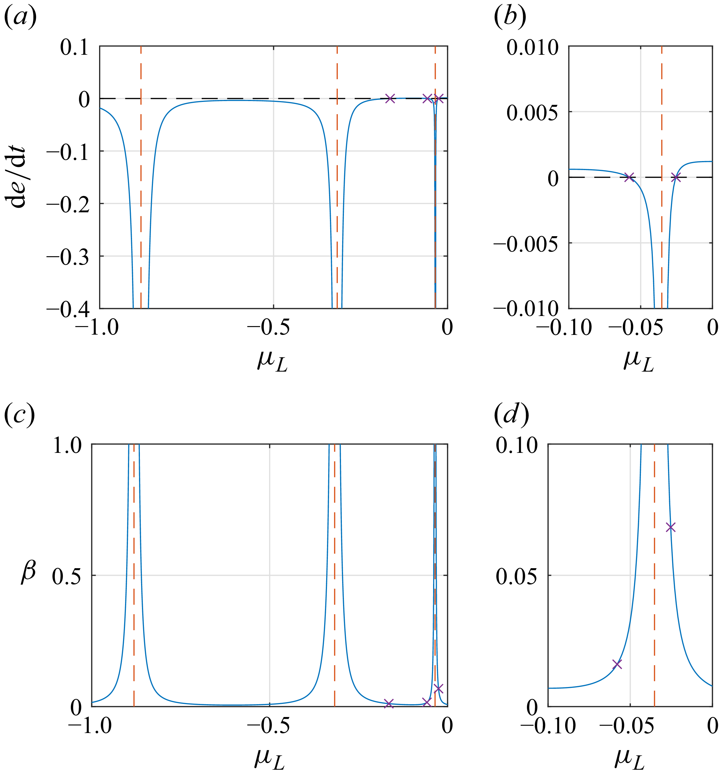
 μL
 de/dt=0
 μL=−0.0352
 Re=140
 U1=(1−y2)(−1.56y6+1.8y4+0.41y2+0.7)
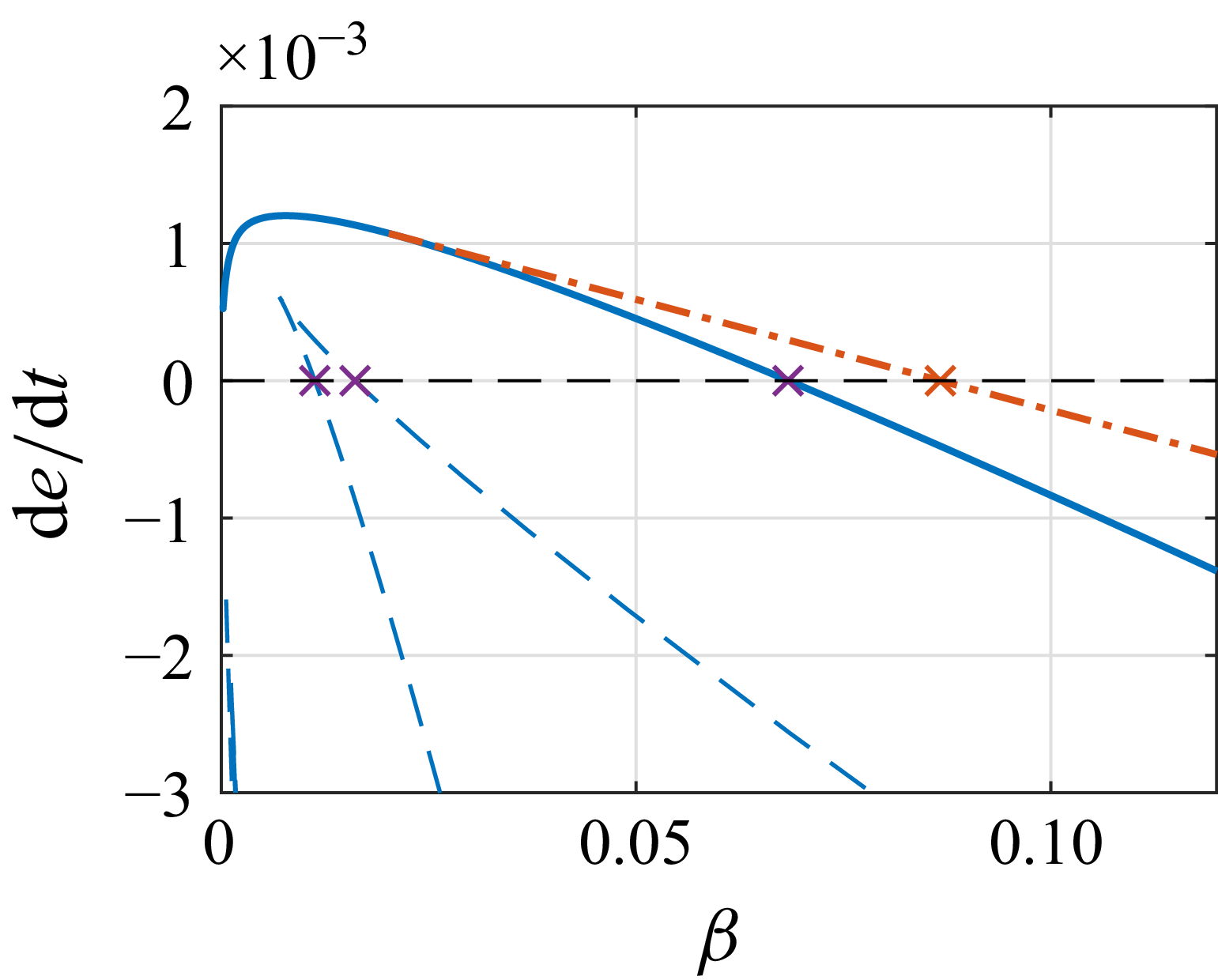
 e˙max(β)
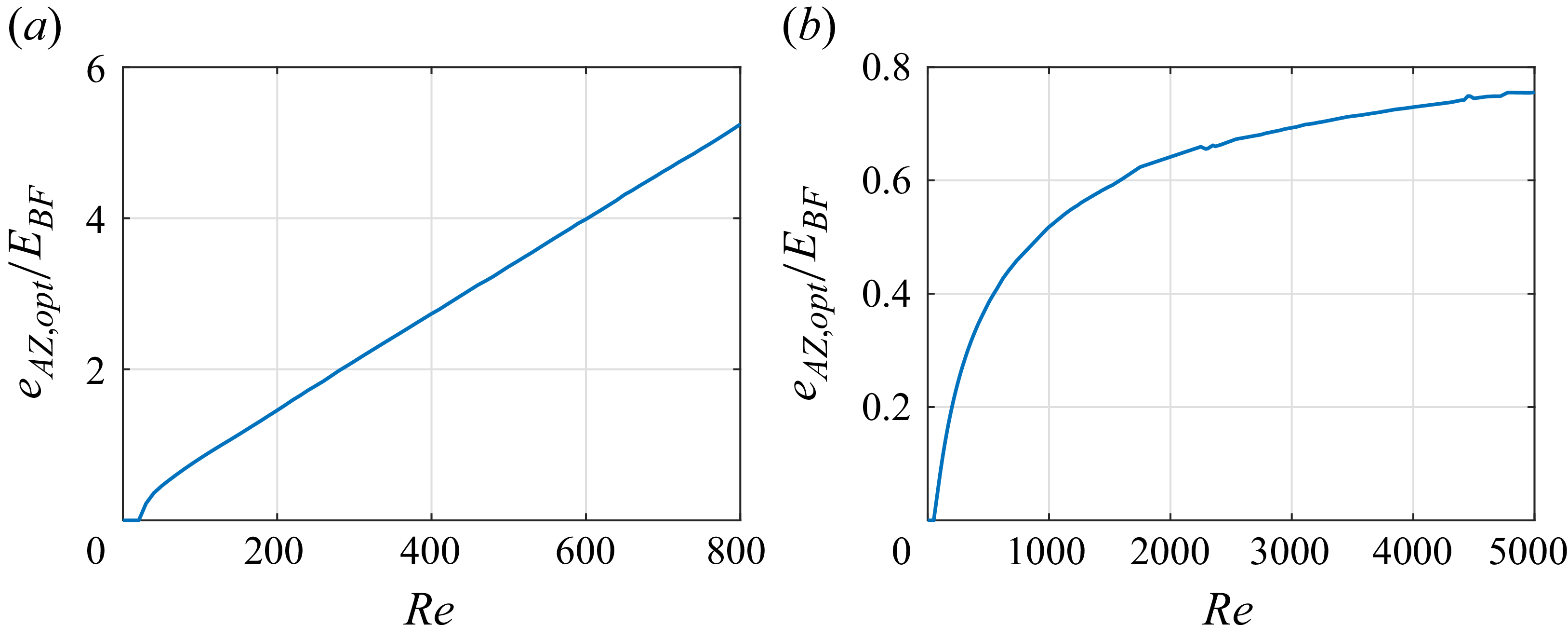


 k3
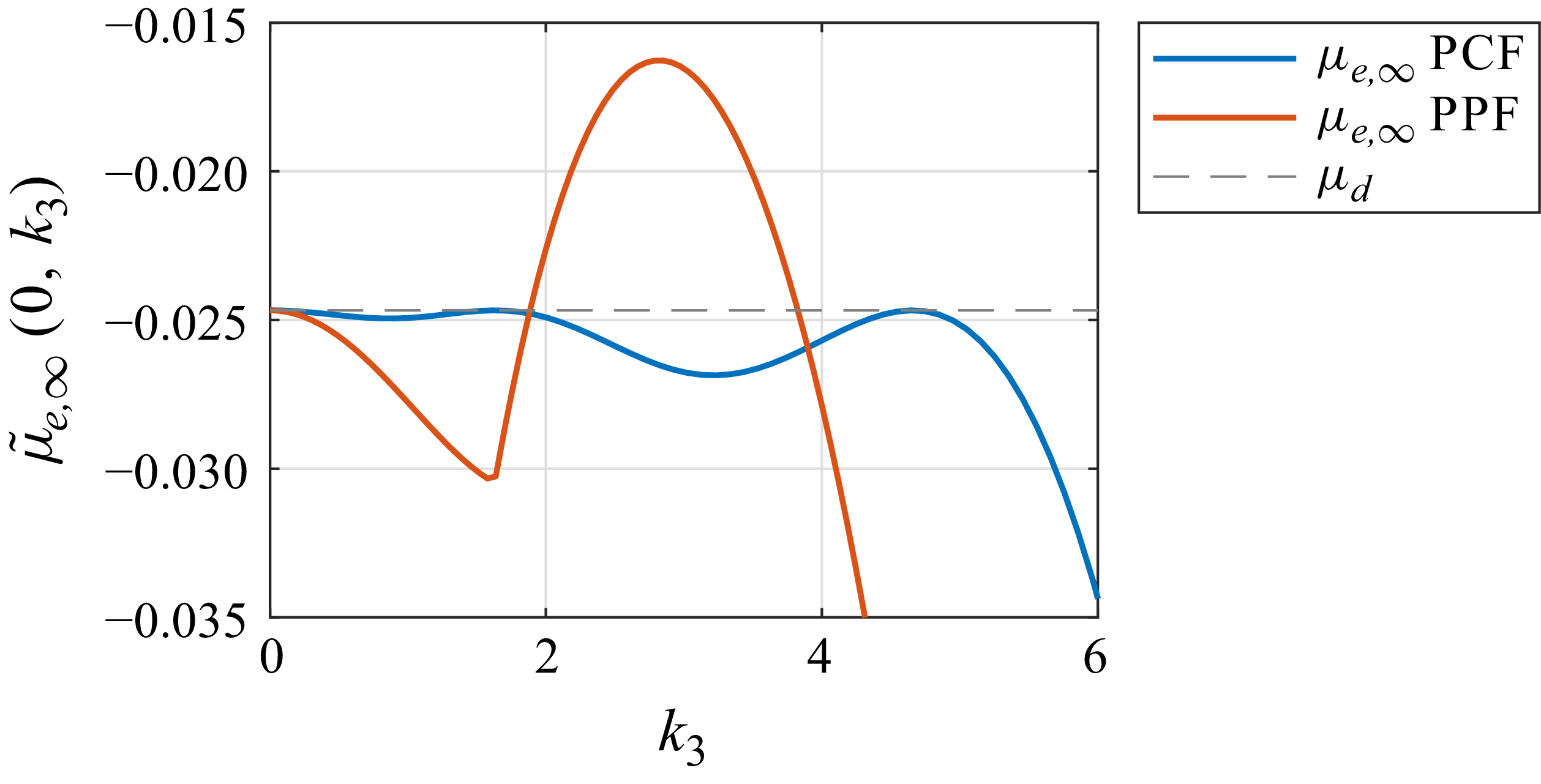
 μ~e,∞
 k3
 Re=200
 k1=0

 k3
 u^1(x2)
 u^2(x2)
 u^3(x2)
 Re=150
 k3=1.977
 Re=200
 k3=2.820
 Re=1400
 k3=2.836
 Re=300
 k3=6.080
 Re=1100
 k3=7.828
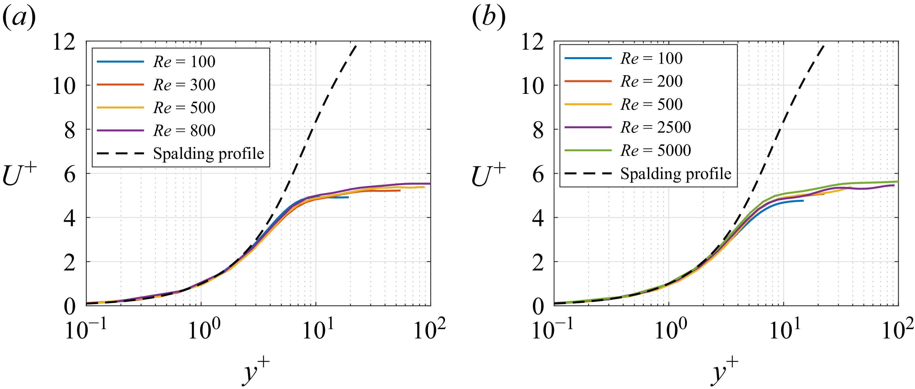
 κ=0.41,C=5.2
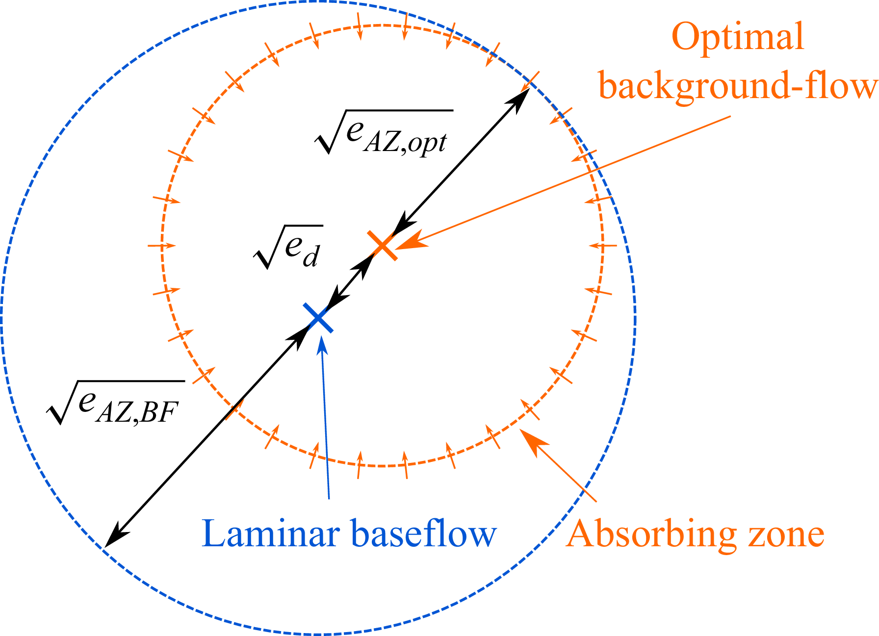
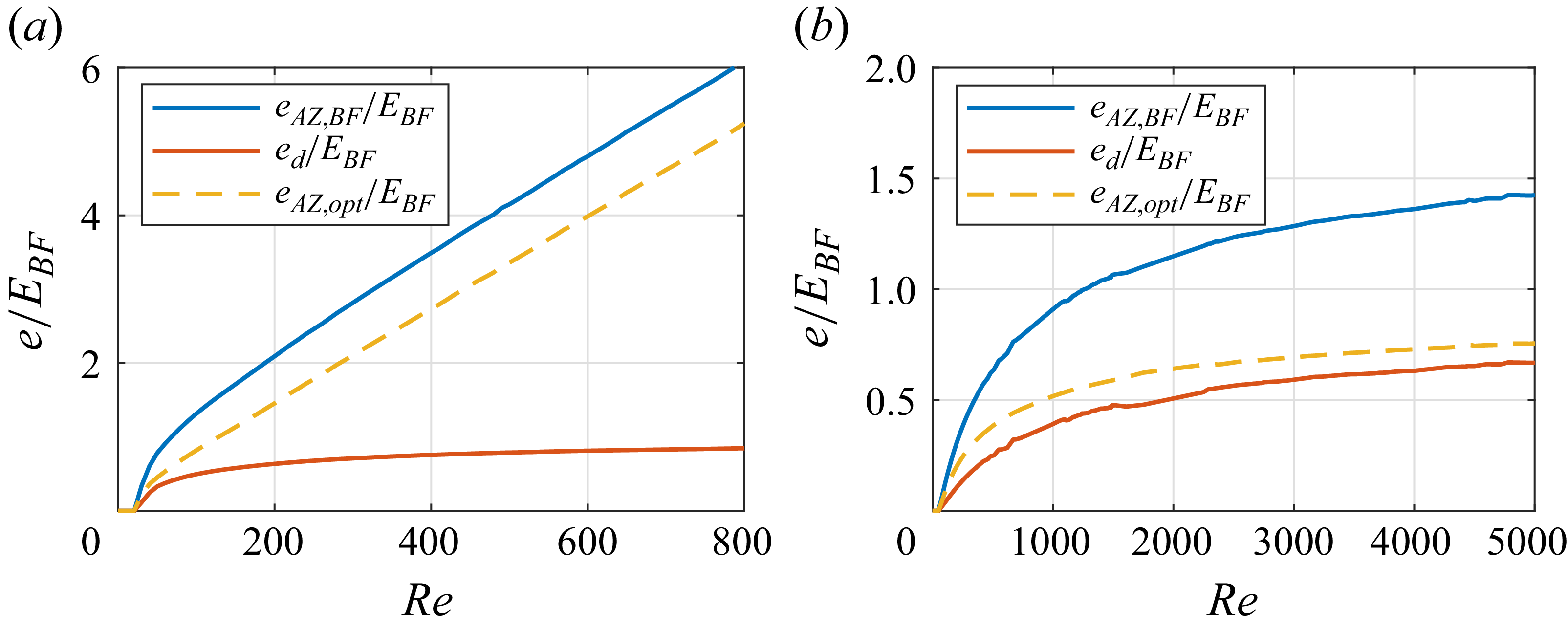
 eAZ, opt
 eAZ, BF
 ed
 EBF
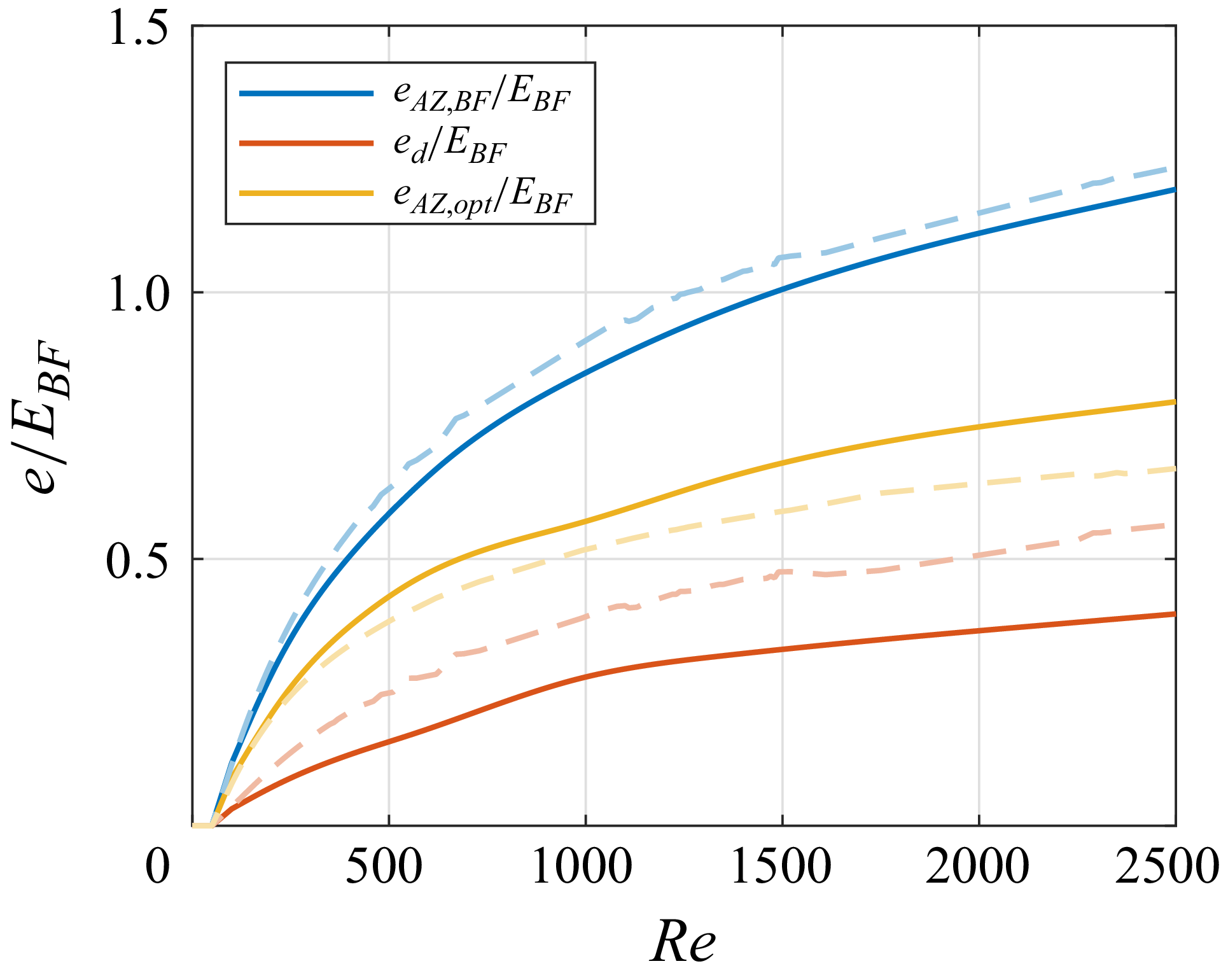
 eAZ,BF
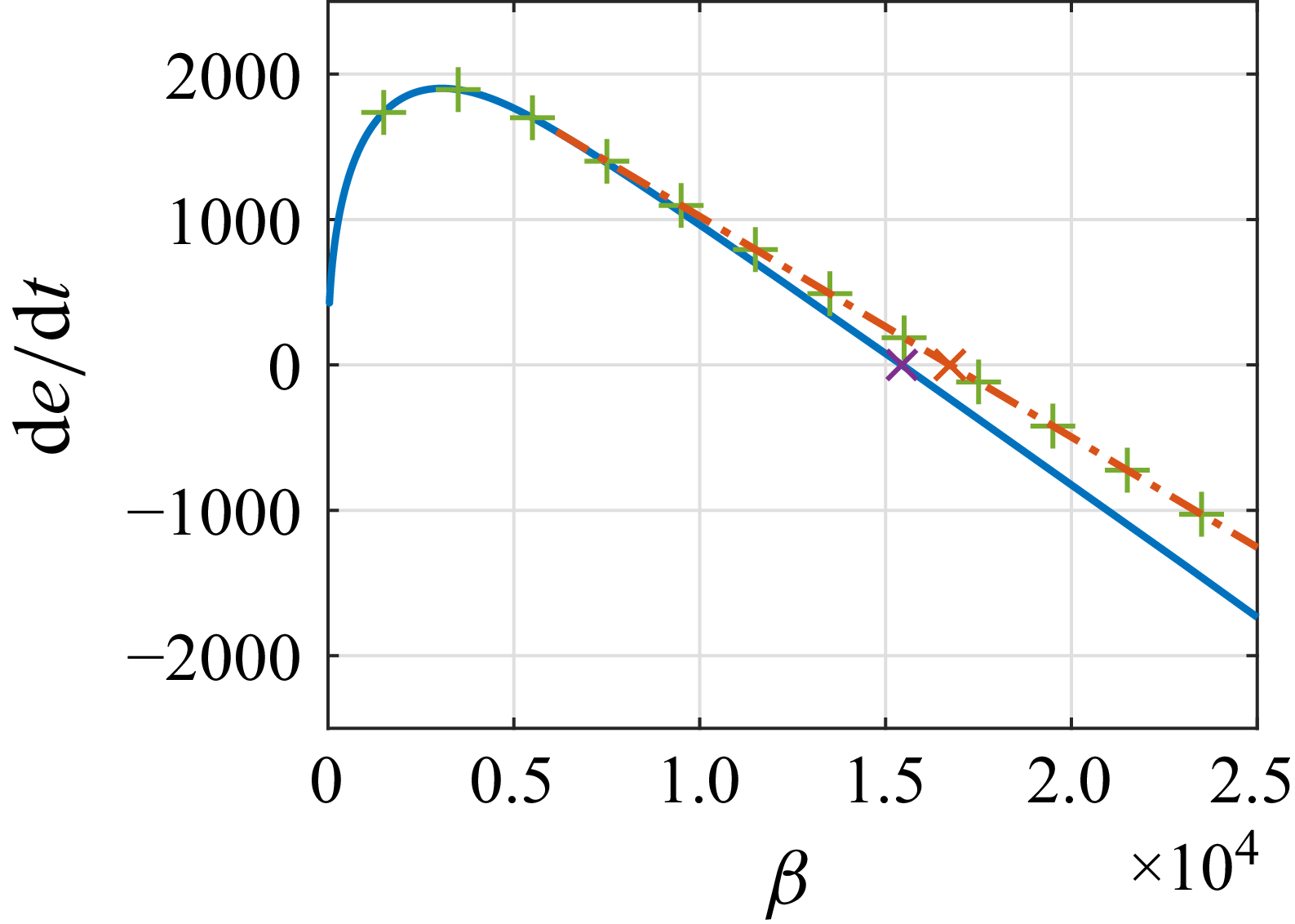
 e˙max(β)
 L=30π
 N=512
 Φ
 etotal
 de/dt
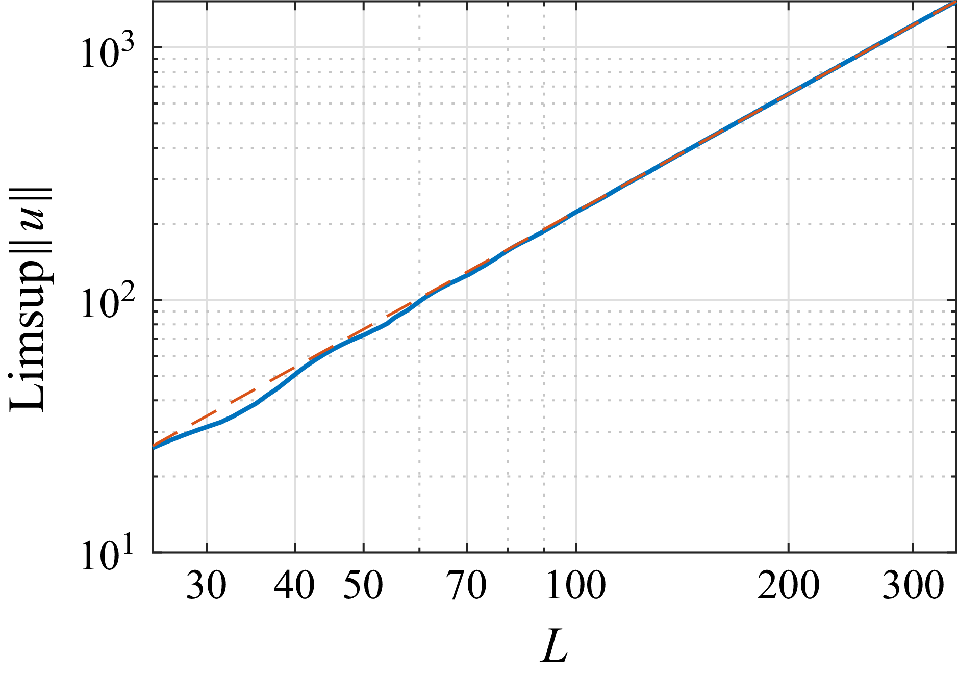
 ‖u‖
 u
 0.1803L1.5470