2.1 Numerical representation of Sumner's journey

Representing Sumner's journey on a programmable map requires accurate numerical knowledge of his path, so we now must sift through what is known (and believed) about his journey in order to create a first visual on a programmable map, using the techniques from our previous work.

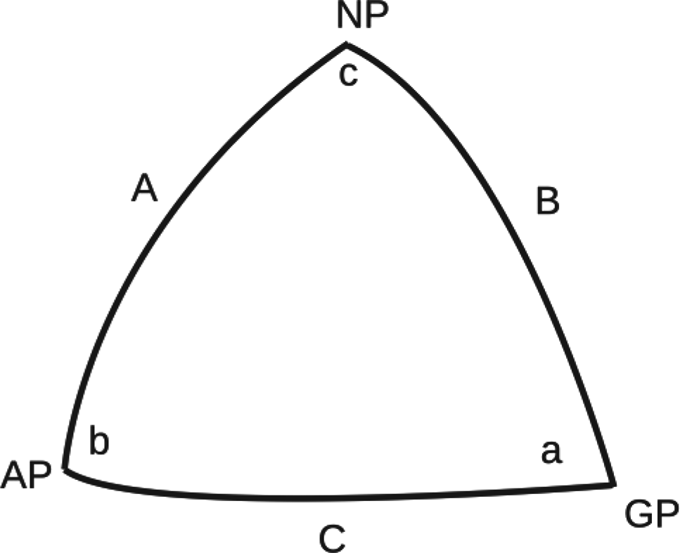
The central CN theme of Sumner's calculations uses a spherical triangle, like that represented by Figure 1.

Figure 1.

Navigational triangle

Here, NP is the north pole, GP the geographical position of the sun, AP the ship's assumed position, c the local hour angle, b the azimuth (or angle) to GP, A the co-latitude of the AP, B the co-latitude of GP, and C the co-altitude of sun. Angle a is not used. The pertinent equation for Sumner's approach is

(1)\begin{equation}\textrm{cos}(c )= \frac{{\textrm{cos}(C )- \textrm{cos}(A )\textrm{cos}(B )}}{{\textrm{sin}(A )\textrm{sin}(B )}}.\end{equation}

which links B from a nautical almanac, C from an alt measurement, and A from the DR lat. Solving for c is related to his lng via the Greenwich Hour Angle (GHA) of the sun (also from a nautical almanac). The parameter A is what Sumner varied in 10′ increments north. To begin with a numerical recreation, we pull statements and figures from a reprint of Sumner's original publication (Vanvaerenbergh and Ifland, Reference Vanvaerenbergh and Ifland2003). In doing so, we immediately found a problem with the rote literature. We thus work up two possible numerical adaptations of the journey, suitable for our classroom lesson.

2.2 Initial problem

Sumner took an alt measurement of the sun on 1837-12-17 at 10:15 am of 12°10′ (page A-15 of Vanvaerenbergh). On page A-14 of the same work, his DR lat was reported as 51°37′. His DR lng was not reported but can be estimated from a map plot presumably produced by Sumner (Plate III of Vanvaerenbergh) to be 6⋅73 W (here −6⋅73°).

His DR lat gives A in Equation (1) and his alt measurement gives C. Side B comes from use of a nautical almanac to find the declination (decl) of the sun at the time of his measurement. Computing lng requires the sun's GHA, also from a nautical almanac. We used online calculators for this, setting them to 10:15 am on 1837-12-17 (183 years ago). We found a decl of 23⋅22°S (NASA, 2020; NOAA, 2020) and a GHA of 334⋅67° (Umland, 2020). With these numbers in place, we were ready for our first numerical recreation at Sumner's journey.

Using Equation (1) as described, we get his ‘longitude from chronometer’ location to be (51⋅62°, −4⋅71°), and his two ‘what-if’ points (each 10′ further north) to be (51⋅79°, −4⋅07°) and (51⋅95°, −3⋅39°).

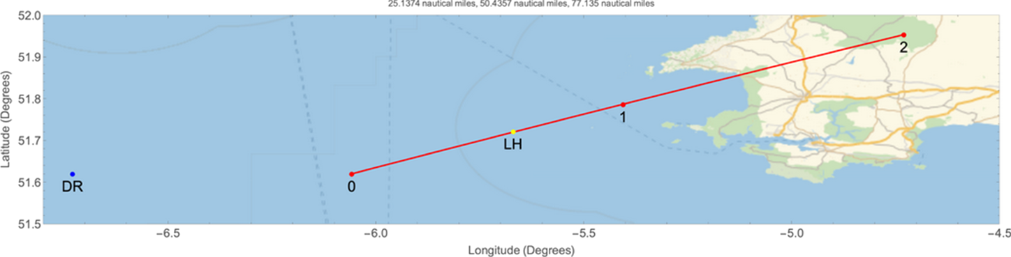
A plot of these points using our mapping technique is shown in Figure 2. In this figure, the blue point labelled ‘DR’ is his supposed DR position and the yellow point labelled ‘LH’ is Smalls lighthouse. The three connected red points produce a line through the three computed positions (here labelled 0, 1 and 2), the plot of which immediately exposes a problem.

Figure 2.

Blue dot: Sumner's original DR position, yellow dot: Smalls lighthouse (LH), Red dots: Sumner's calculated positions (0, 1, and 2)

Sumner claimed that his first calculation (i.e. our point 0) placed his position 9 Nautical Miles (NMi) east of his DR, and the second two (points 1 and 2) 27 and 54 NMi ENE of his DR (hereafter the ‘9 + 27 + 54 check’), respectively. In Figure 2, the first point is 75 NMi and the other two are 100 and 126 NMi from his DR. Also, the line containing the three computed positions supposedly contained Smalls lighthouse.

The entire line is obviously shifted too far to the east, does not contain the lighthouse and is mostly on land near the mainland U.K. We must therefore re-examine the parameters involved prior to bringing this journey into the classroom. We do so in two adaptations presented below, a process made manageable using our programmable mapping technique.

2.3 Adaptation #1

In this adaptation, we assume that Sumner's altitude measurement of 12⋅1° is reliable, as is his DR lat. We wonder, though, if extrapolating back 183 years for the GHA and decl gave correct values. We did our due diligence in this regard, consulting the finest numerical sources we could find (NASA, 2020; NOAA, 2020; PyEphem, 2020; Umland, 2020; Wolfram, 2020), but still had lingering doubts (and realised that implementing our own ephemeris computations is beyond the scope here). We thus allow slight manual variation in these parameters with the goal of having Smalls lighthouse fall on the line, while point 0 moves closer to the DR position. (This is one instance of the value of Sumner's narrative.) Our eventual GHA and decl came out to be 333⋅2° and 23⋅25° (each changed by <1% of those originally stated) to obtain the triple of (51⋅62°,−6⋅06°), (51⋅79°,−5⋅41°) and (51⋅95°,−4⋅73°) for points 0, 1 and 2, respectively, resulting in Figure 3.

Figure 3.

Sumner's computed positions with modified GHA and declination values

As pointed out by a reviewer, this is equivalent to considering that sun may have been observed approximately 6 min later than the time reported by Sumner. We find this small time difference acceptable given the well-known historical hardship of keeping accurate time at sea. This places the lighthouse on the same line as the computed points, but still leaves his original DR position 25 NMi from the first point 0. We thus adjust his DR lng to −6⋅3°, making the distance 9 NMi, 34 NMi and 62 NMi, comfortably close to the 9 + 27 + 54 check, as shown in Figure 4.

Figure 4.

Adaptation #1 of Sumner's calculations. The blue dot (original DR) is 9 NMi from the leftmost red dot, and 34 and 62 NMi from the more rightward red dots

We can proceed in our lesson using the points in Figure 4, but note that it still differs from Sumner's account (Plate III of Vanvaerenbergh), in which Smalls lighthouse falls between points 1 and 2 in the triple, not between 0 and 1 as shown in Figure 4. This suggests Sumner's stated DR lng was too far west by 0⋅43°.

2.4 Adaptation #2

Adaptation #1 allowed for a small and manual changes to the GHA, decl and lng used in Sumner's calculations. While yielding results closer to Sumner's narrative, it still did not produce a close match to it. Manual adjustment of the parameters was difficult, as small changes to one required changes to others, all while attempting to nudge the system closer to Sumner's narrative. This naturally led us to wonder if allowing for small changes in all of Sumner's navigational parameters would lead to another, more optimised adaptation.

We decided on a two-fold goal for a computer-driven minimisation algorithm: (1) minimise the sum of distances to the 9 + 27 + 54 check, and (2) minimise the distance of Smalls lighthouse to the line containing the three computed points. The driving equations are as follows.

First, Equation (1) is solved for c, giving

(2)\begin{equation}c({A,B,C} )= \frac{{180}}{\pi }\left( {\textrm{co}{\textrm{s}^{ - 1}}\left[ {\frac{{\textrm{cos}(C )- \textrm{cos}(A )\textrm{cos}(B )}}{{\textrm{sin}(A )\textrm{sin}(B )}}} \right] + \frac{\pi }{4}} \right),\end{equation}

with the π/4 making the angle determination map friendly, and the 180/π converting to degrees. Next, a distance formula between two (lat, lng) points is defined as (Stackoverflow, 2020)

(3)\begin{align}\begin{array}{*{20}{c}} {d({la{t_1},ln{g_1},la{t_2},ln{g_2}} )= }\\ {6925\;\textrm{si}{\textrm{n}^{ - 1}}\sqrt {\dfrac{1}{2} - \dfrac{1}{2}\textrm{cos}\left[ {\dfrac{\pi }{{180}}({la{t_2} - la{t_1}} )} \right] + \dfrac{1}{2}\textrm{cos}\left[ {\dfrac{\pi }{{180}}la{t_1}} \right]\textrm{cos}\left[ {\dfrac{\pi }{{180}}la{t_2}} \right]\left( {1 - \textrm{cos}\left[ {\dfrac{\pi }{{180}}({ln{g_2}} )} \right]} \right)} ,} \end{array}\end{align}

which returns a distance (in NMi) between points (lat₁,lng₁) and (lat₂,lng₂).

We now define a function to generate a (lat,lng) point based on Sumner's longitude by chronometer technique or

(4)\begin{equation}p({n,decl,alt,gha} )= \left( {51.62 + \frac{{10n}}{{60}},c\left( {90 - \left( {51.62 + \frac{{10n}}{{60}}} \right),90 + decl,90 - alt} \right) + gha} \right).\end{equation}

This is a function of the navigational parameters decl, alt and gha, and n, which is an integer from 0.2, representing the calculated point. Note n = 0 reduces p to

(5)\begin{equation}p({0,decl,alt,gha} )= ({51.62,c({90 - 51.62,90 + decl,90 - alt} )+ gha} ),\end{equation}

which is Sumner's first ‘longitude by chronometer’ calculation. Values of n = 1 and n = 2 give his what-if calculations of being 10′ then 20′ further north.

Lastly, we define a function that returns the distance between a point and a line to be

(6)\begin{equation}g({{x_0},{y_0},a,b,c} )= \frac{{|{a{x_0} + b{y_0} + c} |}}{{\sqrt {{a^2} + {b^2}} }},\end{equation}

where (x ₀,y ₀) is a single point and the line that the form ax + by + c = 0. In use, the point will be the location of Smalls lighthouse, and the line will be the one containing all three of Sumer's computed points.

The function to minimise M sums the distances from Sumner's DR to each of the n = 0, 1 and 2 points, offsetting each term to its respective part in the 9 + 27 + 54 check. It also contains the function g(x ₀,y ₀,a,b,c) from Equation (6) to be

(7)\begin{align} & M(lng,decl,alt,gha) \nonumber\\ & \quad =|d(p(0,25{\cdot}23 + \Delta decl,12{\cdot}16 + \Delta alt,333{\cdot}2 + \Delta gha), (51{\cdot}62, - 6 + \Delta lng))- 9| \nonumber\\ & \qquad +|d(p(1,25{\cdot}23 + \Delta decl,12{\cdot}16 + \Delta alt,333{\cdot}2 + \Delta gha), (51{\cdot}62, - 6 + \Delta lng))- 27| \nonumber\\ & \qquad +|d(p(2,25{\cdot}23 + \Delta decl,12{\cdot}16 + \Delta alt,333{\cdot}2 + \Delta gha),(51{\cdot}62, - 6 + \Delta lng))- 54|\nonumber\\ & \qquad +g(51{\cdot}72, - 5{\cdot}670,a,b,c),\end{align}

which written more compactly becomes

(8)\begin{align} & M(lng,decl,alt,gha)\nonumber\\ & \quad={-}90 + g(51{\cdot}72, - 5{\cdot}670,a,b,c)\nonumber\\ & \qquad+\sum_{n = 0}^2 |d(p(n,25{\cdot}23 + \Delta decl,12{\cdot}16 + \Delta alt,333{\cdot}2 + \Delta gha), (51{\cdot}62, - 6 + \Delta lng))|.\end{align}

Here a, b and c are computed in real time based on a linear fit to Sumer's three computed points as the minimiser runs. Note the (lat,lng) of Smalls lighthouse is known, and a ‘weighting coefficient’ can be placed in front of the g function to vary the importance of this term (we used 2⋅0). We hypothesise that if M can be minimised relative to small changes in the navigation parameters (Δdecl, Δalt, Δgha and Δlng), another suitable adaptation of Sumner's journey may be found.

The ‘Minimise’ function is used in Mathematica (Wolfram, 2020), which gives Δlng = −0⋅488, Δdecl = 0⋅280, Δalt = 0⋅03, and Δgha = 0⋅959. The computed points 0, 1 and 2 come out to be (51⋅62, −6⋅022), (51⋅79, −5⋅48) and (51⋅95, −4⋅92) and are plotted in Figure 5.

Figure 5.

Adaptation #2 of Sumner's journey

We note a nice correspondence with the 9 + 27 + 54 check, here coming in at 9 NMi, 31 NMi, and 54 NMi. Additionally, Smalls lighthouse is very close to the line containing the calculated points. Sumner's supposed DR lng is still further west than that found here at −6⋅26°. This value is similar to that found in Adaptation #1.

We are cautious with our work to this point, as we are proposing a correction to historical data, to make a better match to Sumner's narrative, also noting how our final result is close to that in Bowditch (NIMA, 2015). Our belief in Sumner's altitude measurement (i.e. his sextant skills) in Adaptation #1 is justified, seeing here only a small correction to the altitude parameter. We also note that in the literature, Smalls lighthouse fell between calculated points 1 and 2, not 0 and 1 as arrived at here. We were unable to find a model that replicates this part of his journey.

We now proceed with our classroom lesson, given that we have a model consistent with the description of Sumner's journey. We note again the importance of developing pedagogical lessons in CN.

3.1 Introduction

We naturally start by telling the story, as outlined at the beginning of Section 2 of this work, and on page 9 of Vanvaerenbergh. This is kept as a general overview, including a thorough visual using a standard world map, which alone is an opportunity to expose students to geography beyond their own familiar localities. The sun's visibility at only 10:15 am demonstrates a need for CN beyond the dual chronometer technique, which is typically remembered by students as a technique that only works with the sun at noon (since the sun's apex and thus local time are so easy to discern).

3.2 Initial map plotting

We begin with a manual map plotting exercise, for Sumner's DR position and Smalls lighthouse. Blanks maps are given to the students with axes extending from −4° to −8° in longitude and 48° to 53° in latitude. Such a map roughly exposes the southern coast of Ireland, St. George's Channel and the Pembrokeshire Coast National Park. (To the reader: We quietly note reversing the logic from our numerical adaptations, for our pedagogy: we claim to know the modified DR longitude at the start of the lesson, that came to us only at the end of a numerical adaptation to make the 9 + 27 + 54 check work.)

3.3 Computing ‘longitude by chronometer’

We now approach Sumner's first longitude by chronometer calculation with a close look at Equation (1), which is a formidable one for general education students (but alas we are at a ‘technical’ university). Thanks to Sumner's story, each parameter has a definite meaning. We take careful inventory of what Sumner knew and demonstrate how the entire right-hand side of Equation (1) is known. We work together in class (with calculators) to arrive at c. A targeted discussion now ensues about the relationship between c (the LHA), GHA and longitude. Sumner's story brings a strong sense of purpose to these parameters, as they involve finding his longitude, so ill-fated in the history of navigation. A discussion is often accompanied by the addition of one more arc drawn from the NP in Figure 1, which is that for the Prime Meridian at Greenwich (most conveniently drawn to the east of the NP–GP line shown in Figure 1). With the longitude computed, this point is plotted on the map, with a reference (and check) to the 9 NMi distance between the DR and this computed position, as per the story.

We next return to the general world map, highlighting the Celtic Sea into St. George's Channel, and ask what one would do if they were suspicious of a persistent current from the south. This naturally leads to assuming one's latitude is further north, and that suspicion in one's DR needs no justification, as it is inherently error prone. Some discussion is warranted on the meaning of Sumner's 10′ further north (10 NMi of due north travel on a great circle given the 60 NMi/° rule of thumb). This leads to two more calculations of c involving Equation (1), and two more points plotted on the map. The points are shown to fall on the same line, which requires a pause, as an extremely important idea on CN is emerging: the line of position.

3.4 Live map visual

We now bring out the live programmable map into our lesson. The reader may access the map as well (Bensky, Reference Bensky2020). Note that being a ‘live’ map, the usual zoom and panning controls are both functional.

The map implementation of Sumner's journey is straightforward: it plots all needed points, including Sumner's DR, Smalls lighthouse, the computed points, the sun's GP and the circle of position (COP). Shown in Figure 6, the user clicks on buttons of points they wish to include on the map. When this map is brought up and projected in class for the students, its ‘live’ nature affords the instructor many pedagogical possibilities.

Figure 6.

A live map of Sumner's journey. All map controls (zooming and panning) work, and the user is able to choose which aspects of Sumner's journey to plot. Note here the zoom has made the visible portion of the circle of position appear straight

We initially show Sumner's DR and the sun's GP, which was in Botswana (southern Africa) at the time of Sumner's sighting. We then show the COP, with which the students are already familiar, but this application re-enforces its meaning.

3.5 The line of position

We have found the line of position difficult to get at pedagogically. Circles of position have been presented earlier in the class as an outcome of a sextant shot. We proceed with the COP on the live map as follows.

Using the live map, we display Sumner's calculated positions one by one, but show how we must zoom into the Celtic Sea to see the individual points. This is a very revealing process, as repeated clicking on the map's zoom control causes the GP to eventually leave the map, while the visible portion of the COP in the Celtic Sea begins to straighten as the individual calculated points become distinct.

There are two important concepts in CN that the live map illustrates nicely. First, plotting the DR and the GP on the same map is discussed as forcing some reckoning with issues involving the scale of the map (Schlereth, Reference Schlereth2000; Karl, Reference Karl2011). Using the live map makes this clear, as the thickness of the line used initially to render the COP on a map that includes both the DR and GP positions is as wide as the state of Florida, USA. Second, seeing the COP become straight at high map zoom into a more local swath of ocean clearly shows the origin of a LOP.

The astute student will recognise the emergence of a LOP from a previously learned topic in a calculus course: the LOP is a line tangent to the COP and perpendicular to its radius, which is also the azimuth to the GP. Williams's humour (Williams, Reference Williams1994, page 112) on this revelation serves as an anecdotal point to ponder about the historical development of CN.

3.6 Conclude the lesson

We now discuss Sumner's revelation of the LOP and how he sailed along it to promptly sight the lighthouse, noting that the lighthouse also being on his LOP was only fortuitous. We take time and allow students to ensure their hand-drawn maps correspond with the programmable map, and invariably take some ‘what-if’ questions involving the live map. We note the map will also plot any arbitrary (lat,lng) point by keying it into the text entry box.

Lastly, a comparison between Sumner's journey and the technique of St. Hilaire (Vanvaerenbergh and Ifland, Reference Vanvaerenbergh and Ifland2003) is appropriate. We highlight how both focused on the utility of Equation (1). Sumner's inputs were C and B, while St. Hilaire's were A, c and B. Sumner varied A, while St. Hilaire placed more utility in his DR position (A,c) as his ‘assumed position.’ Sumner wanted to compute c, and St. Hilaire C. While Sumner plotted many computed points, St. Hilaire compared observed and computed (sun) altitudes. Sumner's (mathematical) plots will reveal a LOP while St. Hilaire will use his comparison to move a (sketched) LOP perpendicular to the azimuth, toward or away from the GP. Sumner assumes he is on the computed LOP, and St. Hilaire looks for the intersection of multiple LOPs.