1 Introduction
Rapid distortion theory (RDT) is a powerful analytical tool to describe the evolution of turbulence under strong shear. A significant body of work is available on RDT in the context of single-phase flows (see reviews of Savill (Reference Savill1987) and Hunt, Carruthers & Fung (Reference Hunt, Carruthers and Fung1991)). However, the case of particle-laden turbulence has not been addressed using RDT until now. In this paper, we extend the classic single-phase RDT to strongly sheared turbulence loaded with small heavy particles.
Rapid distortion theory for single-phase flows has a long-standing history. In a seminal paper, Pearson (Reference Pearson1959) derived a closed form for the evolution of turbulent fluctuations due to uniform distortion. The theory provides an analytical description of the evolution of the Fourier modes of the velocity fluctuations. The closed form is made possible by the assumption that the nonlinear inertial effects are negligible compared to the applied distortion. This generated significant interest, particularly in the case of sheared turbulence (Moffatt Reference Moffatt1965; Townsend Reference Townsend1970). Further work by Rogers provided analytical expressions for the Reynolds stress tensor (Rogers Reference Rogers1986; Rogers & Moin Reference Rogers and Moin1987), and the mixing of a passive scalar field (Rogers Reference Rogers1991).
Rapid distortion theory is particularly suited for the analysis of homogeneously sheared turbulence (HST), a fundamental flow that builds up in complexity from homogeneous isotropic turbulence by introducing a mean linear shear. The work done by the mean shear flow produces turbulent kinetic energy and the shear deformation adds to the complexity of the flow structures. As a prototypal turbulent shear flow, a number of studies relied on HST to investigate the effects of turbulence anisotropy (Lee, Kim & Moin Reference Lee, Kim and Moin1990), the emergence of hairpin vortices (Rogers & Moin Reference Rogers and Moin1987), the sweep and ejection mechanisms (Pumir Reference Pumir1996) and the limits of the postulate of local isotropy (Kasbaoui et al.
Reference Kasbaoui, Patel, Koch and Desjardins2017) without contamination by bounding walls. Comparisons with direct numerical simulations (Isaza et al.
Reference Isaza, Warhaft and Collins2009; Kasbaoui et al.
Reference Kasbaoui, Patel, Koch and Desjardins2017) show that, provided the shearing is strong enough, RDT reproduces correctly a wide range of turbulence statistics in HST for a total deformation up to
 $\unicode[STIX]{x1D6E4}t\sim 5$
, where
 $\unicode[STIX]{x1D6E4}$
is the shear rate. The success of RDT is such that many models for single-phase turbulence are evaluated on their ability to recover the RDT limits when tested in HST configuration (Hunt & Carruthers Reference Hunt and Carruthers1990; Hunt et al.
Reference Hunt, Carruthers and Fung1991; Isaza & Collins Reference Isaza and Collins2009; Briard et al.
Reference Briard, Gomez, Mons and Sagaut2016).
In an effort to better understand particle-laden turbulence, many authors studied HST loaded with dispersed particles. In this flow, various numerical studies investigated effects such as turbulence modulation by particle clusters Gualtieri et al. (Reference Gualtieri, Picano, Sardina and Casciola2013), particle shear stress (Shin & Lee Reference Shin and Lee2002), the dispersion of particle pairs (Shen & Yeung Reference Shen and Yeung1997; Ahmed & Elghobashi Reference Ahmed and Elghobashi2001) and the alignment of vortex tubes (Ahmed & Elghobashi Reference Ahmed and Elghobashi2000). However, it remains to link particle-laden HST to a theoretical grounding such as RDT.
The challenge in extending RDT to particle-laden turbulence arises from the strong interaction between the particulate and gaseous phases. Particles cluster in turbulence owing to their preferential sampling of the straining regions of the flow (Maxey Reference Maxey1987; Squires & Eaton Reference Squires and Eaton1991; Eaton & Fessler Reference Eaton and Fessler1994; Kasbaoui et al.
Reference Kasbaoui, Koch, Subramanian and Desjardins2015; Sumbekova et al.
Reference Sumbekova, Cartellier, Aliseda and Bourgoin2017). In a recent study (Kasbaoui, Koch & Desjardins Reference Kasbaoui, Koch and Desjardins2019), we showed that shear may be a precursor to a cascade of instabilities called ‘the route to clustering’ that leads to the formation of clusters orders of magnitude larger than the particle diameter. Elghobashi and coworkers showed from direct numerical simulations that dispersed particles in the two-way coupling limit, modify the alignment of vortex tubes in HST, increase the turbulent kinetic energy and dissipation rate and may cause further anisotropic alteration of turbulence at small scales in the sedimentation direction (Elghobashi & Truesdell Reference Elghobashi and Truesdell1992; Ahmed & Elghobashi Reference Ahmed and Elghobashi2000, Reference Ahmed and Elghobashi2001). This modulation is strong when the mass loading
 $M=\unicode[STIX]{x1D70C}_{p}\langle \unicode[STIX]{x1D719}\rangle /\unicode[STIX]{x1D70C}_{f}$
is order unity, where
 $\unicode[STIX]{x1D70C}_{p}$
and
 $\unicode[STIX]{x1D70C}_{f}$
are the particles and fluid densities and
 $\langle \unicode[STIX]{x1D719}\rangle$
is the average particle volume fraction. In the present study, we focus on gaseous flows loaded with solid particles or liquid droplets. Because of the large density ratio of aerosols (
 $\unicode[STIX]{x1D70C}_{p}/\unicode[STIX]{x1D70C}_{f}=O(10^{3})$
), the coupling between the two phases is strong even at relatively dilute concentrations (
 $\langle \unicode[STIX]{x1D719}\rangle <10^{-3}$
). Unlike in single-phase RDT, where the kinematic distortion is the only process at play, a two-way coupled RDT for particle-laden HST needs to capture the dynamic anisotropic modulation the aerosols and gas exert on each other as they are sheared. Since even a linearized treatment shows a drastic growth of sinusoidal volume fraction perturbations in simple shear (Kasbaoui et al.
Reference Kasbaoui, Koch, Subramanian and Desjardins2015), one may expect interesting results when a range of scales exists as is the case in turbulence.
This paper is organized as follows. We start by presenting the governing equation for sheared particle-laden flows in § 2. To make the analysis tractable, we focus on particles with small inertia, for which the velocity field is given as an expansion in Stokes number (Ferry & Balachandar Reference Ferry and Balachandar2001). Then, we derive the extended RDT in § 3. We show that the classical RDT is recovered in the limit of vanishing mass loading and provide a closed form for the two-phase case. In § 4, we compare the predictions of the theory to fully nonlinear, Euler–Lagrange numerical simulations of particle-laden HST.
2 Governing equations
An incompressible Newtonian gas of density
 $\unicode[STIX]{x1D70C}_{f}$
and viscosity
 $\unicode[STIX]{x1D707}_{f}$
is loaded with monodisperse solid particles (or liquid droplets) of density
 $\unicode[STIX]{x1D70C}_{p}$
and diameter
 $d_{p}$
at the average volume fraction
 $\langle \unicode[STIX]{x1D719}\rangle$
. These particles experience a gravitational force and a hydrodynamic force equal to the Stokes drag (Maxey & Riley Reference Maxey and Riley1983)
 $$\begin{eqnarray}\displaystyle & \displaystyle \frac{\text{d}\boldsymbol{x}_{p}^{i}}{\text{d}t}=\boldsymbol{u}_{p}^{i}, & \displaystyle\end{eqnarray}$$
 $$\begin{eqnarray}\displaystyle & \displaystyle \frac{\text{d}\boldsymbol{u}_{p}^{i}}{\text{d}t}=\frac{\boldsymbol{u}_{f}(\boldsymbol{x}_{p}^{i},t)-\boldsymbol{u}_{p}^{i}}{\unicode[STIX]{x1D70F}_{p}}+\boldsymbol{g}, & \displaystyle\end{eqnarray}$$
where
 $\boldsymbol{x}_{p}^{i}$
and
 $\boldsymbol{u}_{p}^{i}$
are the Lagrangian position and velocity of particle ‘
 $i$
’,
 $\unicode[STIX]{x1D70F}_{p}=\unicode[STIX]{x1D70C}_{p}d_{p}^{2}/(18\unicode[STIX]{x1D707}_{f})$
is the particle response time,
 $\boldsymbol{u}_{f}$
is the fluid velocity and
 $\boldsymbol{g}$
is the gravitational acceleration. Other hydrodynamic forces such as the Basset history force and the lift force can be neglected due to the large density ratio between solid particles or liquid droplets and the carrier gas. Particle–particle interactions such as collisions and detailed hydrodynamic coupling are also negligible for semi-dilute aerosols. The carrier gas satisfies the Navier–Stokes equations
 $$\begin{eqnarray}\displaystyle & \displaystyle \unicode[STIX]{x1D735}\boldsymbol{\cdot }\boldsymbol{u}_{f}=0, & \displaystyle\end{eqnarray}$$
 $$\begin{eqnarray}\displaystyle & \displaystyle \unicode[STIX]{x1D70C}_{f}\frac{\unicode[STIX]{x2202}\boldsymbol{u}_{f}}{\unicode[STIX]{x2202}t}+\unicode[STIX]{x1D70C}_{f}\boldsymbol{u}_{f}\boldsymbol{\cdot }\unicode[STIX]{x1D735}\boldsymbol{u}_{f}=-\unicode[STIX]{x1D735}p+\unicode[STIX]{x1D707}_{f}\unicode[STIX]{x1D6FB}^{2}\boldsymbol{u}_{f}+\unicode[STIX]{x1D70C}_{f}\boldsymbol{g}+\unicode[STIX]{x1D70C}_{p}\unicode[STIX]{x1D719}\frac{\boldsymbol{u}_{p}-\boldsymbol{u}_{f}}{\unicode[STIX]{x1D70F}_{p}}, & \displaystyle\end{eqnarray}$$
where
 $\boldsymbol{u}_{p}$
is the Eulerian particle velocity field.
In Euler–Lagrange approaches, individual particles are tracked using (2.1) and (2.2) and Eulerian quantities such as the local volume fraction
 $\unicode[STIX]{x1D719}$
and particle velocity field
 $\boldsymbol{u}_{p}$
are determined a posteriori. Euler–Euler approaches rely on solving partial differential equations for the Eulerian quantities directly and are preferred for analytical treatments. According to Druzhinin (Reference Druzhinin1995), the particle evolution equations (2.1) and (2.2) lead to the following conservation equations for the particle mass and momentum
 $$\begin{eqnarray}\displaystyle & \displaystyle \unicode[STIX]{x1D70C}_{p}\frac{\unicode[STIX]{x2202}\unicode[STIX]{x1D719}}{\unicode[STIX]{x2202}t}+\unicode[STIX]{x1D70C}_{p}\unicode[STIX]{x1D735}\boldsymbol{\cdot }\left(\unicode[STIX]{x1D719}\boldsymbol{u}_{p}\right)=0, & \displaystyle\end{eqnarray}$$
 $$\begin{eqnarray}\displaystyle & \displaystyle \unicode[STIX]{x1D70C}_{p}\frac{\unicode[STIX]{x2202}(\unicode[STIX]{x1D719}\boldsymbol{u}_{p})}{\unicode[STIX]{x2202}t}+\unicode[STIX]{x1D70C}_{p}\unicode[STIX]{x1D735}\boldsymbol{\cdot }\left(\unicode[STIX]{x1D719}\boldsymbol{u}_{p}\boldsymbol{u}_{p}\right)=\unicode[STIX]{x1D70C}_{p}\unicode[STIX]{x1D719}\boldsymbol{g}+\unicode[STIX]{x1D70C}_{p}\unicode[STIX]{x1D719}\frac{\boldsymbol{u}_{f}-\boldsymbol{u}_{p}}{\unicode[STIX]{x1D70F}_{p}}. & \displaystyle\end{eqnarray}$$
While being conceptually and numerically simpler, this approach has been verified in many studies (Druzhinin Reference Druzhinin1995; Zhang & Prosperetti Reference Zhang and Prosperetti1997; Druzhinin Reference Druzhinin2001) to yield agreement with the Euler–Lagrange approach in semi-dilute particle-laden flows. This approach is also restricted to small and moderate Stokes numbers since particle-trajectory crossing effects, which are not captured by this Euler–Euler formulation, become significant at high Stokes numbers (Desjardins, Fox & Villedieu Reference Desjardins, Fox and Villedieu2008b ).
It is seen from the two momentum equations (2.4) and (2.6) that the mass loading
 $M=\unicode[STIX]{x1D70C}_{p}/\unicode[STIX]{x1D70C}_{f}\langle \unicode[STIX]{x1D719}\rangle$
is a measure of the coupling strength between the phases. In the one-way coupling regime, i.e.
 $M\ll 1$
, perturbations in the gas velocity drive inhomogeneities in the particle phase, but there is no feedback to the gas. For aerosols, this effectively takes place for volume fractions below
 $10^{-6}$
. In the semi-dilute regime, i.e.
 $10^{-5}<\langle \unicode[STIX]{x1D719}\rangle <10^{-3}$
corresponding to
 $M=O(1)$
, the particle feedback cannot be neglected due to the large density ratio
 $\unicode[STIX]{x1D70C}_{p}/\unicode[STIX]{x1D70C}_{f}=O(10^{3})$
.
In addition to the mass loading, the nature of the particle-laden flow is determined by the Stokes number
 $St=\unicode[STIX]{x1D70F}_{p}/T_{f}$
, where
 $T_{f}$
is a characteristic fluid time scale. The Stokes number is a measure of the particle inertia. Particles with
 $St=0$
act like tracers, whereas particles with
 $St\rightarrow \infty$
have an uncorrelated ballistic motion. Particles with
 $St=O(1)$
have a motion correlated with the fluid but the non-vanishing slip velocity leads to strong clustering (Squires & Eaton Reference Squires and Eaton1991; Eaton & Fessler Reference Eaton and Fessler1994).
To further simplify the analysis, we constrain the study to particles with small but non-zero inertia. For such particles, it is possible to approximate the particle velocity field in terms of fluid quantities and gravity. The expansion in particle relaxation time truncated to first order (Maxey Reference Maxey1987; Druzhinin Reference Druzhinin1994; Ferry & Balachandar Reference Ferry and Balachandar2001) yields
 $$\begin{eqnarray}\boldsymbol{u}_{p}=\boldsymbol{u}_{f}+\boldsymbol{U}_{g}-\unicode[STIX]{x1D70F}_{p}\left(\frac{\unicode[STIX]{x2202}\boldsymbol{u}_{f}}{\unicode[STIX]{x2202}t}+(\boldsymbol{u}_{f}+\boldsymbol{U}_{g})\boldsymbol{\cdot }\unicode[STIX]{x1D735}\boldsymbol{u}_{f}\right)+O(\unicode[STIX]{x1D70F}_{p}^{2}),\end{eqnarray}$$
where
 $\boldsymbol{U}_{g}=\unicode[STIX]{x1D70F}_{p}\boldsymbol{g}$
is the particle settling velocity. The studies of Ferry & Balachandar (Reference Ferry and Balachandar2002) in turbulent channel flow and Ferry & Balachandar (Reference Ferry and Balachandar2001) and Rani & Balachandar (Reference Rani and Balachandar2003) in isotropic homogeneous turbulence show this approximation holds for
 $St_{\unicode[STIX]{x1D702}}=\unicode[STIX]{x1D70F}_{p}/\unicode[STIX]{x1D70F}_{\unicode[STIX]{x1D702}}<0.3$
, where
 $\unicode[STIX]{x1D70F}_{\unicode[STIX]{x1D702}}$
is the Kolmogorov time scale. Using (2.7), Shotorban & Balachandar (Reference Shotorban and Balachandar2009) performed two-way coupled simulations of decaying particle-laden homogeneous isotropic turbulence and obtained kinetic energy and dissipation rate that match Euler–Lagrange simulations for
 $St_{\unicode[STIX]{x1D702}}<0.25$
. In homogeneously sheared turbulence, the existence of a second flow time scale,
 $T_{f}=\unicode[STIX]{x1D6E4}^{-1}$
, introduces a second Stokes number based on the shear rate
 $St_{\unicode[STIX]{x1D6E4}}=\unicode[STIX]{x1D6E4}\unicode[STIX]{x1D70F}_{p}$
. Both Stokes numbers
 $St_{\unicode[STIX]{x1D702}}$
and
 $St_{\unicode[STIX]{x1D6E4}}$
need to be small in order for the expansion (2.7) to be applicable. Our recent simulations (Kasbaoui et al.
Reference Kasbaoui, Patel, Koch and Desjardins2017) of sheared sedimenting particles in the two-way coupling regime show favourable comparisons with the full Eulerian equations for the shear-based Stokes number
 $St_{\unicode[STIX]{x1D6E4}}=\unicode[STIX]{x1D70F}_{p}\unicode[STIX]{x1D6E4}\sim 0.1$
. Hence, we will consider this expansion applicable for
 $St_{\unicode[STIX]{x1D6E4}}<0.1$
and
 $St_{\unicode[STIX]{x1D702}}<0.3$
.
With the expansion (2.7), the governing equations can be recast in the following form
 $$\begin{eqnarray}\displaystyle & \displaystyle \unicode[STIX]{x1D735}\boldsymbol{\cdot }\boldsymbol{u}_{f}=0, & \displaystyle\end{eqnarray}$$
 $$\begin{eqnarray}\displaystyle & \displaystyle \left(\unicode[STIX]{x1D70C}_{f}+\unicode[STIX]{x1D70C}_{p}\unicode[STIX]{x1D719}\right)\left(\frac{\unicode[STIX]{x2202}\boldsymbol{u}_{f}}{\unicode[STIX]{x2202}t}+\boldsymbol{u}_{f}\boldsymbol{\cdot }\unicode[STIX]{x1D735}\boldsymbol{u}_{f}\right)=-\unicode[STIX]{x1D735}p+\unicode[STIX]{x1D707}_{f}\unicode[STIX]{x1D6FB}^{2}\boldsymbol{u}_{f}\hspace{80.00012pt} & \displaystyle \nonumber\\ \displaystyle & \displaystyle \hspace{115.00017pt}\quad +\,\left(\unicode[STIX]{x1D70C}_{f}+\unicode[STIX]{x1D70C}_{p}\unicode[STIX]{x1D719}\right)\boldsymbol{g}-\unicode[STIX]{x1D70C}_{p}\unicode[STIX]{x1D719}\boldsymbol{U}_{g}\boldsymbol{\cdot }\unicode[STIX]{x1D735}\boldsymbol{u}_{f}, & \displaystyle\end{eqnarray}$$
 $$\begin{eqnarray}\displaystyle & \displaystyle \frac{\unicode[STIX]{x2202}\unicode[STIX]{x1D719}}{\unicode[STIX]{x2202}t}+\left(\boldsymbol{u}_{f}+\boldsymbol{U}_{g}-\unicode[STIX]{x1D70F}_{p}\left(\frac{\unicode[STIX]{x2202}\boldsymbol{u}_{f}}{\unicode[STIX]{x2202}t}+(\boldsymbol{u}_{f}+\boldsymbol{U}_{g})\boldsymbol{\cdot }\unicode[STIX]{x1D735}\boldsymbol{u}_{f}\right)\right)\boldsymbol{\cdot }\unicode[STIX]{x1D735}\unicode[STIX]{x1D719}=\unicode[STIX]{x1D70F}_{p}\unicode[STIX]{x1D719}\unicode[STIX]{x1D735}\boldsymbol{u}_{f}\boldsymbol{ : }\unicode[STIX]{x1D735}\boldsymbol{u}_{f}. & \displaystyle\end{eqnarray}$$
These equations resemble those of a variable density fluid of density
 $\unicode[STIX]{x1D70C}_{f}+\unicode[STIX]{x1D70C}_{p}\unicode[STIX]{x1D719}$
, although differences exist. The most notable differences can be seen in the volume fraction equation (2.10), in which the right-hand side contains a source of volume fraction fluctuations due to preferential concentration. This term can be expressed as the difference between the second tensor invariants of the straining and rotation tensors. Hence, in regions where the straining exceeds the rotation, this term causes exponential accumulation of particles. In the opposite scenario, this term acts as a sink. Moreover, the volume fraction field is convected at the particle velocity rather than that of the fluid.
Now, we consider that the flow is subject to homogeneous shear. Without loss of generality, we define
 $x_{1}$
,
 $x_{2}$
and
 $x_{3}$
as the streamwise, shear and spanwise directions, respectively. The driving shear flow is expressed as
 $\unicode[STIX]{x1D6E4}x_{2}\boldsymbol{e}_{1}$
. It is often useful to rewrite the previous equations in terms of the fluctuating velocity
 $\boldsymbol{u}_{f}^{\prime }=\boldsymbol{u}_{f}-\unicode[STIX]{x1D6E4}x_{2}\boldsymbol{e}_{1}$
, leading to
 $$\begin{eqnarray}\displaystyle & \displaystyle \unicode[STIX]{x1D735}\boldsymbol{\cdot }\boldsymbol{u}_{f}^{\prime }=0, & \displaystyle\end{eqnarray}$$
 $$\begin{eqnarray}\displaystyle & \displaystyle \left(\unicode[STIX]{x1D70C}_{f}+\unicode[STIX]{x1D70C}_{p}\unicode[STIX]{x1D719}\right)\left(\frac{\unicode[STIX]{x2202}\boldsymbol{u}_{f}^{\prime }}{\unicode[STIX]{x2202}t}+\unicode[STIX]{x1D6E4}x_{2}\frac{\unicode[STIX]{x2202}\boldsymbol{u}_{f}^{\prime }}{\unicode[STIX]{x2202}x_{1}}+\boldsymbol{u}_{f}^{\prime }\boldsymbol{\cdot }\unicode[STIX]{x1D735}\boldsymbol{u}_{f}^{\prime }+\unicode[STIX]{x1D6E4}u_{f,2}^{\prime }\boldsymbol{e}_{1}\right)\hspace{60.00009pt} & \displaystyle \nonumber\\ \displaystyle & \displaystyle \qquad =-\unicode[STIX]{x1D735}p+\unicode[STIX]{x1D707}_{f}\unicode[STIX]{x1D6FB}^{2}\boldsymbol{u}_{f}^{\prime }+\,\left(\unicode[STIX]{x1D70C}_{f}+\unicode[STIX]{x1D70C}_{p}\unicode[STIX]{x1D719}\right)\boldsymbol{g}-\unicode[STIX]{x1D70C}_{p}\unicode[STIX]{x1D719}\left(\boldsymbol{U}_{g}\boldsymbol{\cdot }\unicode[STIX]{x1D735}\boldsymbol{u}_{f}^{\prime }+\unicode[STIX]{x1D6E4}U_{g,2}\boldsymbol{e}_{1}\right), & \displaystyle\end{eqnarray}$$
 $$\begin{eqnarray}\displaystyle & \displaystyle \frac{\unicode[STIX]{x2202}\unicode[STIX]{x1D719}}{\unicode[STIX]{x2202}t}+\unicode[STIX]{x1D6E4}x_{2}\frac{\unicode[STIX]{x2202}\unicode[STIX]{x1D719}}{\unicode[STIX]{x2202}x_{1}}+\boldsymbol{u}_{p}^{\prime }\boldsymbol{\cdot }\unicode[STIX]{x1D735}\unicode[STIX]{x1D719}=\unicode[STIX]{x1D719}\unicode[STIX]{x1D70F}_{p}\unicode[STIX]{x1D735}\boldsymbol{u}_{f}^{\prime }\boldsymbol{ : }\unicode[STIX]{x1D735}\boldsymbol{u}_{f}^{\prime }+2\unicode[STIX]{x1D719}\unicode[STIX]{x1D6E4}\unicode[STIX]{x1D70F}_{p}\frac{\unicode[STIX]{x2202}u_{f,2}^{\prime }}{\unicode[STIX]{x2202}x_{1}}, & \displaystyle\end{eqnarray}$$
where the deviation of the particle velocity from simple shear
 $\boldsymbol{u}_{p}^{\prime }=\boldsymbol{u}_{p}-\unicode[STIX]{x1D6E4}x_{2}\boldsymbol{e}_{1}$
is given by
 $$\begin{eqnarray}\displaystyle \boldsymbol{u}_{p}^{\prime } & = & \displaystyle \boldsymbol{u}_{f}^{\prime }+\boldsymbol{U}_{g}\nonumber\\ \displaystyle & & \displaystyle -\,\unicode[STIX]{x1D70F}_{p}\left(\frac{\unicode[STIX]{x2202}\boldsymbol{u}_{f}^{\prime }}{\unicode[STIX]{x2202}t}+\unicode[STIX]{x1D6E4}x_{2}\frac{\unicode[STIX]{x2202}\boldsymbol{u}_{f}^{\prime }}{\unicode[STIX]{x2202}x_{1}}+\left(\boldsymbol{u}_{f}^{\prime }+\boldsymbol{U}_{g}\right)\boldsymbol{\cdot }\unicode[STIX]{x1D735}\boldsymbol{u}_{f}^{\prime }+\unicode[STIX]{x1D6E4}\left(u_{f,2}+U_{g,2}\right)\boldsymbol{e}_{1}\right).\end{eqnarray}$$
In this representation, the convection by homogeneous shear terms
 $\unicode[STIX]{x1D6E4}x_{2}\unicode[STIX]{x2202}/\unicode[STIX]{x2202}x_{1}$
appear explicitly. These terms are also known as the distortion terms. In spectral space, they induce turning of the wave vector of the Fourier modes (Thomson Reference Thomson1887; Moffatt Reference Moffatt1965; Kasbaoui et al.
Reference Kasbaoui, Koch, Subramanian and Desjardins2015) towards a direction parallel to the velocity gradient. The distortion of turbulence leads to the elongation of vortex tubes (Rogers & Moin Reference Rogers and Moin1987) and their alignment in a direction nearly perpendicular to the velocity gradient (Sukheswalla, Vaithianathan & Collins Reference Sukheswalla, Vaithianathan and Collins2013).
RDT is applicable when the shearing is strong so that the distortion term in the momentum equation exceeds in magnitude the nonlinear convection. Formally, this is expressed as
 $$\begin{eqnarray}\frac{\Vert \unicode[STIX]{x1D6E4}x_{2}\unicode[STIX]{x2202}\boldsymbol{u}_{f}^{\prime }/\unicode[STIX]{x2202}x_{1}\Vert }{\Vert \boldsymbol{u}_{f}^{\prime }\boldsymbol{\cdot }\unicode[STIX]{x1D735}\boldsymbol{u}_{f}^{\prime }\Vert }\sim \unicode[STIX]{x1D6E4}\unicode[STIX]{x1D70F}_{f}=S^{\ast }\gg 1,\end{eqnarray}$$
where
 $\unicode[STIX]{x1D70F}_{f}=\langle u_{f,i}^{\prime }u_{f,i}^{\prime }\rangle /\unicode[STIX]{x1D716}$
is the large eddy turnover time and
 $\unicode[STIX]{x1D716}$
is the dissipation rate. It is clear that RDT will be applicable in the limit of large shear numbers
 $S^{\ast }=\unicode[STIX]{x1D6E4}\langle u_{f,i}^{\prime }u_{f,i}^{\prime }\rangle /\unicode[STIX]{x1D716}$
.
For expansion (2.7) to remain valid, both the shear and turbulent Stokes numbers need to be small. The shear Stokes number can be written as
 $$\begin{eqnarray}St_{\unicode[STIX]{x1D6E4}}=\unicode[STIX]{x1D6E4}\unicode[STIX]{x1D70F}_{p}=\unicode[STIX]{x1D6E4}\unicode[STIX]{x1D70F}_{f}\frac{\unicode[STIX]{x1D70F}_{p}}{\unicode[STIX]{x1D70F}_{\unicode[STIX]{x1D702}}}\frac{\unicode[STIX]{x1D70F}_{\unicode[STIX]{x1D702}}}{\unicode[STIX]{x1D70F}_{f}}\sim \frac{S^{\ast }St_{\unicode[STIX]{x1D702}}}{\sqrt{Re_{l}}},\end{eqnarray}$$
where
 $Re_{l}=\unicode[STIX]{x1D70C}_{f}\unicode[STIX]{x1D716}l^{2}/(\langle u_{f,i}^{\prime }u_{f,i}^{\prime }\rangle \unicode[STIX]{x1D707}_{f})$
is the large scale Reynolds number, and
 $l$
denotes the integral length scale (Pope Reference Pope2001). Thus, for
 $St_{\unicode[STIX]{x1D702}}<0.3$
and sufficiently large Reynolds number, the condition
 $St_{\unicode[STIX]{x1D6E4}}<0.1$
can be satisfied even for large
 $S^{\ast }$
.
The assumption of rapid distortion along with a Boussinesq approximation allows linearization of the governing equations. Note that velocity fluctuations drive volume fraction variations that are order
 $1/S^{\ast }$
smaller than the mean volume fraction and thus
 $\unicode[STIX]{x1D719}^{\prime }=\unicode[STIX]{x1D719}-\langle \unicode[STIX]{x1D719}\rangle \ll 1$
. Performing an expansion in
 $1/S^{\ast }$
and retaining the leading-order terms leads to the following equations:
 $$\begin{eqnarray}\displaystyle & \displaystyle \unicode[STIX]{x1D735}\boldsymbol{\cdot }\boldsymbol{u}_{f}^{\prime }=0, & \displaystyle\end{eqnarray}$$
 $$\begin{eqnarray}\displaystyle & \displaystyle \frac{\unicode[STIX]{x2202}\boldsymbol{u}_{f}^{\prime }}{\unicode[STIX]{x2202}t}+\unicode[STIX]{x1D6E4}x_{2}\frac{\unicode[STIX]{x2202}\boldsymbol{u}_{f}^{\prime }}{\unicode[STIX]{x2202}x_{1}}+\unicode[STIX]{x1D6E4}u_{f,2}^{\prime }\boldsymbol{e}_{1}=-\frac{1}{\unicode[STIX]{x1D70C}_{m}}\unicode[STIX]{x1D735}p^{\prime }+\frac{\unicode[STIX]{x1D707}_{f}}{\unicode[STIX]{x1D70C}_{m}}\unicode[STIX]{x1D6FB}^{2}\boldsymbol{u}_{f}^{\prime }\hspace{20.00003pt} & \displaystyle \nonumber\\ \displaystyle & \displaystyle \hspace{125.00018pt}+\,\frac{\unicode[STIX]{x1D70C}_{p}\unicode[STIX]{x1D719}^{\prime }}{\unicode[STIX]{x1D70C}_{m}}\boldsymbol{g}-\frac{\unicode[STIX]{x1D70C}_{p}\langle \unicode[STIX]{x1D719}\rangle }{\unicode[STIX]{x1D70C}_{m}}\boldsymbol{U}_{g}\boldsymbol{\cdot }\unicode[STIX]{x1D735}\boldsymbol{u}_{f}^{\prime }, & \displaystyle\end{eqnarray}$$
 $$\begin{eqnarray}\displaystyle & \displaystyle \frac{\unicode[STIX]{x2202}\unicode[STIX]{x1D719}^{\prime }}{\unicode[STIX]{x2202}t}+\unicode[STIX]{x1D6E4}x_{2}\frac{\unicode[STIX]{x2202}\unicode[STIX]{x1D719}^{\prime }}{\unicode[STIX]{x2202}x_{1}}+\boldsymbol{U}_{g}\boldsymbol{\cdot }\unicode[STIX]{x1D735}\unicode[STIX]{x1D719}=2\langle \unicode[STIX]{x1D719}\rangle \unicode[STIX]{x1D6E4}\unicode[STIX]{x1D70F}_{p}\frac{\unicode[STIX]{x2202}u_{f,2}^{\prime }}{\unicode[STIX]{x2202}x_{1}}, & \displaystyle\end{eqnarray}$$
where
 $p^{\prime }=p+\unicode[STIX]{x1D70C}_{m}\boldsymbol{g}\boldsymbol{\cdot }\boldsymbol{x}$
is a reduced pressure and
 $\unicode[STIX]{x1D70C}_{m}=\unicode[STIX]{x1D70C}_{f}+\unicode[STIX]{x1D70C}_{p}\langle \unicode[STIX]{x1D719}\rangle$
is an effective mixture density. Equations (2.17), (2.18) and (2.19) constitute the RDT governing equations in physical space. It is worthwhile to transform these equations to spectral space. Such a representation allows an understanding of the distortion of turbulence in terms of its spectral content. Applying a Fourier transform to the RDT equations yields
 $$\begin{eqnarray}\displaystyle & \displaystyle \boldsymbol{k}\boldsymbol{\cdot }\hat{\boldsymbol{u}}_{f}=0, & \displaystyle\end{eqnarray}$$
 $$\begin{eqnarray}\displaystyle & \displaystyle \frac{\unicode[STIX]{x2202}\hat{\boldsymbol{u}}_{f}}{\unicode[STIX]{x2202}t}-\unicode[STIX]{x1D6E4}k_{1}\frac{\unicode[STIX]{x2202}\hat{\boldsymbol{u}}_{f}}{\unicode[STIX]{x2202}k_{2}}+\unicode[STIX]{x1D6E4}\hat{u} _{f,2}\boldsymbol{e}_{1}=-\frac{\text{i}\,\boldsymbol{k}}{\unicode[STIX]{x1D70C}_{m}}\hat{p}-\frac{\unicode[STIX]{x1D707}_{f}}{\unicode[STIX]{x1D70C}_{m}}k^{2}\hat{\boldsymbol{u}}_{f}+\frac{\unicode[STIX]{x1D70C}_{p}\hat{\unicode[STIX]{x1D719}}}{\unicode[STIX]{x1D70C}_{m}}\boldsymbol{g}-\frac{\unicode[STIX]{x1D70C}_{p}\langle \unicode[STIX]{x1D719}\rangle }{\unicode[STIX]{x1D70C}_{m}}\text{i}\boldsymbol{U}_{g}\boldsymbol{\cdot }\boldsymbol{k}\hat{\boldsymbol{u}}_{f}, & \displaystyle\end{eqnarray}$$
 $$\begin{eqnarray}\displaystyle & \displaystyle \frac{\unicode[STIX]{x2202}\hat{\unicode[STIX]{x1D719}}}{\unicode[STIX]{x2202}t}-\unicode[STIX]{x1D6E4}k_{1}\frac{\unicode[STIX]{x2202}\hat{\unicode[STIX]{x1D719}}}{\unicode[STIX]{x2202}k_{2}}+\text{i}\boldsymbol{U}_{g}\boldsymbol{\cdot }\boldsymbol{k}\hat{\unicode[STIX]{x1D719}}=2\langle \unicode[STIX]{x1D719}\rangle \unicode[STIX]{x1D6E4}\unicode[STIX]{x1D70F}_{p}\text{i}k_{1}\hat{u} _{f,2}, & \displaystyle\end{eqnarray}$$
where
 $\hat{\boldsymbol{u}}_{f}$
and
 $\hat{\unicode[STIX]{x1D753}}$
are the Fourier coefficients associated with the mode of wave vector
 $\boldsymbol{k}=(k_{1},k_{2},k_{3})$
and wavenumber
 $k=\sqrt{k_{1}^{2}+k_{2}^{2}+k_{3}^{2}}$
, defined as
 $$\begin{eqnarray}\displaystyle & \displaystyle \hat{\boldsymbol{u}}_{f}(t,\boldsymbol{k})=\frac{1}{\left(2\unicode[STIX]{x03C0}\right)^{3/2}}\int _{\boldsymbol{x}\in \mathbb{R}^{3}}\boldsymbol{u}_{f}^{\prime }(t,\boldsymbol{x})\exp \left(-\text{i}\,\boldsymbol{k}\boldsymbol{\cdot }\boldsymbol{x}\right)\text{d}\boldsymbol{x}, & \displaystyle\end{eqnarray}$$
 $$\begin{eqnarray}\displaystyle & \displaystyle \hat{\unicode[STIX]{x1D719}}(t,\boldsymbol{k})=\frac{1}{\left(2\unicode[STIX]{x03C0}\right)^{3/2}}\int _{\boldsymbol{x}\in \mathbb{R}^{3}}\unicode[STIX]{x1D719}^{\prime }(t,\boldsymbol{x})\exp \left(-\text{i}\,\boldsymbol{k}\boldsymbol{\cdot }\boldsymbol{x}\right)\text{d}\boldsymbol{x}. & \displaystyle\end{eqnarray}$$
The solenoidal condition (2.20) ensures that the pressure acts solely in the wave normal direction
 $\boldsymbol{k}$
. The forces driving the flow are obtained by projecting the momentum equation into the directions perpendicular to the wave vector,
 $\unicode[STIX]{x1D6FF}_{ij}-k_{i}k_{j}/k$
, resulting in
 $$\begin{eqnarray}\displaystyle & & \displaystyle \frac{\unicode[STIX]{x2202}\hat{\boldsymbol{u}}_{f}}{\unicode[STIX]{x2202}t}-\unicode[STIX]{x1D6E4}k_{1}\frac{\unicode[STIX]{x2202}\hat{\boldsymbol{u}}_{f}}{\unicode[STIX]{x2202}k_{2}}+\unicode[STIX]{x1D6E4}\hat{u} _{f,2}\left(\unicode[STIX]{x1D644}-2\frac{\boldsymbol{k}\boldsymbol{k}}{k^{2}}\right)\boldsymbol{\cdot }\boldsymbol{e}_{1}+\frac{\unicode[STIX]{x1D70C}_{p}\langle \unicode[STIX]{x1D719}\rangle }{\unicode[STIX]{x1D70C}_{m}}\text{i}\boldsymbol{U}_{g}\boldsymbol{\cdot }\boldsymbol{k}\hat{\boldsymbol{u}}_{f}\nonumber\\ \displaystyle & & \displaystyle \quad =-\frac{\unicode[STIX]{x1D707}_{f}}{\unicode[STIX]{x1D70C}_{m}}k^{2}\hat{\boldsymbol{u}}_{f}+\frac{\unicode[STIX]{x1D70C}_{p}\hat{\unicode[STIX]{x1D719}}}{\unicode[STIX]{x1D70C}_{m}}\left(\unicode[STIX]{x1D644}-\frac{\boldsymbol{k}\boldsymbol{k}}{k^{2}}\right)\boldsymbol{\cdot }\boldsymbol{g}.\end{eqnarray}$$
In the previous equations, the distortion term appears as
 $\unicode[STIX]{x1D6E4}k_{1}\unicode[STIX]{x2202}/\unicode[STIX]{x2202}k_{2}$
in the transformed equations. This term causes a transfer of energy in the Fourier space from the large scale modes to short modes parallel to the velocity gradient direction. A key step in the RDT derivation for rapidly sheared flows consists in solving along the characteristic
 $\text{d}k_{2}/\text{d}t=-k_{1}\unicode[STIX]{x1D6E4}$
in spectral space (Thomson Reference Thomson1887). This effectively means that Fourier modes turn towards a direction parallel to the velocity gradient. Note that, in single-phase flows, a single rotating Fourier mode is a complete solution to the nonlinear Navier Stokes equations (Craik & Criminale Reference Craik and Criminale1986), indicating that these modes are fundamental solutions for homogeneously sheared flows. Finally, the complete set of equations for the rotating Fourier modes are
 $$\begin{eqnarray}\displaystyle & \displaystyle \frac{\text{d}\hat{\boldsymbol{u}}_{f}}{\text{d}t}+\unicode[STIX]{x1D6E4}\hat{u} _{f,2}\left(\unicode[STIX]{x1D644}-2\frac{\boldsymbol{k}\boldsymbol{k}}{k^{2}}\right)\boldsymbol{\cdot }\boldsymbol{e}_{1}+\frac{\unicode[STIX]{x1D70C}_{p}\langle \unicode[STIX]{x1D719}\rangle }{\unicode[STIX]{x1D70C}_{m}}\text{i}\boldsymbol{U}_{g}\boldsymbol{\cdot }\boldsymbol{k}\hat{\boldsymbol{u}}_{f} & \displaystyle \nonumber\\ \displaystyle & \displaystyle \quad =-\frac{\unicode[STIX]{x1D707}_{f}}{\unicode[STIX]{x1D70C}_{m}}k^{2}\hat{\boldsymbol{u}}_{f}+\frac{\unicode[STIX]{x1D70C}_{p}\hat{\unicode[STIX]{x1D719}}}{\unicode[STIX]{x1D70C}_{m}}\left(\unicode[STIX]{x1D644}-\frac{\boldsymbol{k}\boldsymbol{k}}{k^{2}}\right)\boldsymbol{\cdot }\boldsymbol{g}, & \displaystyle\end{eqnarray}$$
 $$\begin{eqnarray}\displaystyle & \displaystyle \frac{\text{d}\hat{\unicode[STIX]{x1D719}}}{\text{d}t}+\text{i}\boldsymbol{U}_{g}\boldsymbol{\cdot }\boldsymbol{k}\hat{\unicode[STIX]{x1D719}}=2\langle \unicode[STIX]{x1D719}\rangle \unicode[STIX]{x1D6E4}\unicode[STIX]{x1D70F}_{p}\text{i}k_{1}\hat{u} _{f,2}, & \displaystyle\end{eqnarray}$$
 $$\begin{eqnarray}\displaystyle & \displaystyle \boldsymbol{k}(t)=\left(k_{1},k_{2},k_{3}\right)=(k_{1,0},k_{2,0}-k_{1,0}\unicode[STIX]{x1D6E4}t,k_{3,0}). & \displaystyle\end{eqnarray}$$
Defining the linear operator
 $\unicode[STIX]{x1D653}(\boldsymbol{k}_{0},t)$
solution to the evolution equations (2.26), (2.27) and (2.28), any fluctuations
 $\boldsymbol{u}_{f}^{\prime }(\boldsymbol{x},t)$
and
 $\unicode[STIX]{x1D719}^{\prime }(\boldsymbol{x},t)$
can be computed from the spectral content at a time origin
 $t=0$
(equations (2.23) and (2.24)) using
 $$\begin{eqnarray}\unicode[STIX]{x1D74C}(\boldsymbol{x},t)=\int \int \int \left\{\unicode[STIX]{x1D653}(\boldsymbol{k}_{0},t)\hat{\unicode[STIX]{x1D74C}}_{0}\exp \left(\text{i}\,\boldsymbol{k}(t)\boldsymbol{\cdot }\boldsymbol{x}\right)\right\}\text{d}\,\boldsymbol{k}_{0},\end{eqnarray}$$
where
 $\unicode[STIX]{x1D74C}=(\boldsymbol{u}_{f}^{\prime },\unicode[STIX]{x1D719}^{\prime })^{\text{T}}$
are the physical space fluctuations and
 $\hat{\unicode[STIX]{x1D74C}}_{0}=(\hat{\boldsymbol{u}}_{f,0},\hat{\unicode[STIX]{x1D719}}_{0})^{\text{T}}$
are their Fourier amplitudes at the initial time.
3 The rapid distortion matrix for particle-laden turbulence
The purpose of RDT is to find a solution operator
 $\unicode[STIX]{x1D653}$
that maps the later turbulence spectrum to the initial one. When the particle volume fraction is null (i.e. in a single-phase flow), the solution operator can be obtained analytically (Pearson Reference Pearson1959; Moffatt Reference Moffatt1965; Townsend Reference Townsend1970). However, this will not be the case in general. In what follows, we introduce notions of the theory of linear functional equations that prove useful for the treatment of the particle-laden case. We will apply this approach to the single-phase case first and show that we recover the classical single-phase RDT results. Then we will present the extension to particle-laden flows.
First, we write the general two-phase equations (2.26) and (2.27) in the following matrix form
 $$\begin{eqnarray}\displaystyle \frac{\text{d}\hat{\unicode[STIX]{x1D712}}}{\text{d}t}+\left(\unicode[STIX]{x1D63F}+\unicode[STIX]{x1D651}+\unicode[STIX]{x1D642}+\unicode[STIX]{x1D63E}\right)\hat{\unicode[STIX]{x1D712}}=0, & & \displaystyle\end{eqnarray}$$
 $$\begin{eqnarray}\displaystyle \hat{\unicode[STIX]{x1D712}}(t=0)=\left(\hat{u} _{f,1}(0),\hat{u} _{f,2}(0),\hat{u} _{f,3}(0),\hat{\unicode[STIX]{x1D719}}(0)\right)^{\text{T}}=\hat{\unicode[STIX]{x1D712}}_{0}, & & \displaystyle\end{eqnarray}$$
where
 $\unicode[STIX]{x1D63F}$
,
 $\unicode[STIX]{x1D651}$
,
 $\unicode[STIX]{x1D642}$
and
 $\unicode[STIX]{x1D63E}$
are the distortion, viscous diffusion, gravitational settling and coupling operators, respectively, given as


The operators above have a time dependence incurred by the shear induced variation of
 $k_{2}=k_{2,0}-\unicode[STIX]{x1D6E4}k_{1}t$
and
 $k=\sqrt{k_{1}^{2}+k_{2}^{2}+k_{3}^{2}}$
. The distortion operator is responsible for the change of magnitude of the spectral modes due to the rotation of the wave vectors. The viscous diffusion operator acts only on the fluid velocity and causes the damping of fluid velocity fluctuations by viscosity. The gravitational settling describes the mass and momentum transport due to the settling of particles. The coupling operator captures the effects that each phase has on the other: the imbalance of fluid strain and rotation, i.e. preferential concentration, promotes the growth of volume fraction perturbations, which lead to a spatially varying gravitational loading on the fluid. Notice that unlike the other block-diagonal operators, the coupling operator contains only off-diagonal components responsible for coupling the dynamics of the fluid velocity and the particle volume fraction.
The time dependence of the operators renders the task of finding a solution to (3.1) vastly more complicated than for constant operators. In the spirit of the general theory of linear functional equations (Bellman Reference Bellman1997), we will focus on solving the differential system (3.1) for the variable time matrix
 $\unicode[STIX]{x1D653}(t)$
with an initial condition
 $\unicode[STIX]{x1D653}(t=0)=\unicode[STIX]{x1D644}$
, i.e.
 $$\begin{eqnarray}\displaystyle & \displaystyle \frac{\text{d}\unicode[STIX]{x1D653}}{\text{d}t}+\left(\unicode[STIX]{x1D63F}+\unicode[STIX]{x1D651}+\unicode[STIX]{x1D642}+\unicode[STIX]{x1D63E}\right)\unicode[STIX]{x1D653}=0, & \displaystyle\end{eqnarray}$$
 $$\begin{eqnarray}\displaystyle & \displaystyle \unicode[STIX]{x1D653}(t=0)=\unicode[STIX]{x1D644}. & \displaystyle\end{eqnarray}$$
Finding the solution
 $\unicode[STIX]{x1D653}(t)$
to the general problem leads to a specific solution
 $\hat{\unicode[STIX]{x1D712}}(t)$
that incorporates the initial conditions
 $\hat{\unicode[STIX]{x1D712}}_{0}$
following the simple multiplication rule
 $\hat{\unicode[STIX]{x1D712}}(t)=\unicode[STIX]{x1D653}(t)\hat{\unicode[STIX]{x1D712}}_{0}$
.
3.1 Single-phase case
In the single-phase setting (
 $\langle \unicode[STIX]{x1D719}\rangle =0$
), the coupling and gravitational settling operators are zero. Assuming an inviscid fluid for now, the fluctuations associated with the initial mode
 $\boldsymbol{k}_{0}$
are completely determined by the distortion
 $$\begin{eqnarray}\frac{\text{d}\unicode[STIX]{x1D653}}{\text{d}t}+\unicode[STIX]{x1D63F}\unicode[STIX]{x1D653}=0.\end{eqnarray}$$
Given the simple form of the operator
 $\unicode[STIX]{x1D63F}$
, solving the system (3.9) can be done by hand, albeit tediously, with the initial condition
 $\unicode[STIX]{x1D653}=\unicode[STIX]{x1D644}$
. Doing so, one arrives to a solution equal to the classical single-phase RDT operator,
 $\unicode[STIX]{x1D653}=\unicode[STIX]{x1D63C}$
, where
 $$\begin{eqnarray}\displaystyle & \displaystyle \unicode[STIX]{x1D63C}(\boldsymbol{k}_{0},t)=\left(\begin{array}{@{}cccc@{}}\,1 & {\displaystyle \frac{k_{0}^{2}}{k_{1}^{2}+k_{3}^{2}}}\left(-{\displaystyle \frac{k_{3}^{2}}{k_{0}^{2}}}P+{\displaystyle \frac{k_{1}^{2}}{k_{0}^{2}}}Q\right) & 0 & 0\,\\ \,0 & {\displaystyle \frac{k_{0}^{2}}{k^{2}}} & 0 & 0\,\\ \,0 & {\displaystyle \frac{k_{1}k_{3}}{k_{1}^{2}+k_{3}^{2}}}\left(P+Q\right) & 1 & 0\,\\ \,0 & 0 & 0 & 1\,\end{array}\right), & \displaystyle\end{eqnarray}$$
 $$\begin{eqnarray}\displaystyle & \displaystyle P=\frac{k_{0}^{2}}{k_{1}\sqrt{k_{1}^{2}+k_{z}^{2}}}\left(\arctan \unicode[STIX]{x1D6FC}-\arctan \unicode[STIX]{x1D70F}\right), & \displaystyle\end{eqnarray}$$
 $$\begin{eqnarray}\displaystyle & \displaystyle Q=\frac{\unicode[STIX]{x1D6E4}t\left(k_{0}^{2}-2k_{2,0}^{2}+k_{1}k_{2,0}\unicode[STIX]{x1D6E4}t\right)}{k^{2}}, & \displaystyle\end{eqnarray}$$
 $$\begin{eqnarray}\displaystyle & \displaystyle \unicode[STIX]{x1D6FC}=\frac{k_{2,0}}{\sqrt{k_{1}^{2}+k_{3}^{2}}}, & \displaystyle\end{eqnarray}$$
 $$\begin{eqnarray}\displaystyle & \displaystyle \unicode[STIX]{x1D70F}=\frac{k_{2}}{\sqrt{k_{1}^{2}+k_{3}^{2}}}. & \displaystyle\end{eqnarray}$$
This form has been derived by Pearson (Reference Pearson1959), although earlier results can be traced to Kelvin (Thomson Reference Thomson1887).
The inclusion of viscous effects, although trivial, serves to illustrate how a full solution can be built by adding the effects of the operators one at a time. Keeping the viscous diffusion operator, we now seek to solve an equation that supersedes (3.9),
 $$\begin{eqnarray}\frac{\text{d}\unicode[STIX]{x1D653}}{\text{d}t}+\left(\unicode[STIX]{x1D63F}+\unicode[STIX]{x1D651}\right)\unicode[STIX]{x1D653}=0.\end{eqnarray}$$
To find a solution to the viscous RDT equation above that extends the inviscid result, consider the new matrix
 $\unicode[STIX]{x1D654}=\unicode[STIX]{x1D63C}^{-1}\unicode[STIX]{x1D653}$
. Injecting this form in (3.15) yields an equation for
 $\unicode[STIX]{x1D654}$
,
 $$\begin{eqnarray}\frac{\text{d}\unicode[STIX]{x1D654}}{\text{d}t}+\unicode[STIX]{x1D63C}^{-1}\unicode[STIX]{x1D651}\unicode[STIX]{x1D63C}\unicode[STIX]{x1D654}=0,\end{eqnarray}$$
with the initial condition
 $\unicode[STIX]{x1D654}(0)=\unicode[STIX]{x1D644}$
. The inverse of the RDT matrix is simply
 $\unicode[STIX]{x1D63C}^{-1}(\boldsymbol{k}_{0},t)=\unicode[STIX]{x1D63C}(\boldsymbol{k}(t),-t)$
, which states that the distortion of the mode
 $\boldsymbol{k}(t)$
backwards in time recovers the mode
 $\boldsymbol{k}_{0}$
. Because of the particular diagonal structure of
 $\unicode[STIX]{x1D651}$
, it commutes with the distortion operator
 $\unicode[STIX]{x1D63C}$
, which leads to
 $\unicode[STIX]{x1D63C}^{-1}\unicode[STIX]{x1D651}\unicode[STIX]{x1D63C}=\unicode[STIX]{x1D651}$
. Physically, this means that the viscous diffusion acts in the same way in the laboratory reference frame and the distorted one.
Because
 $\unicode[STIX]{x1D651}$
is a diagonal operator, the solution to (3.16) is a diagonal matrix such that
 $$\begin{eqnarray}\displaystyle & \displaystyle \unicode[STIX]{x1D654}(t)=\text{diag}\left(\text{e}^{-\unicode[STIX]{x1D6FC}_{1}},\text{e}^{-\unicode[STIX]{x1D6FC}_{1}},\text{e}^{-\unicode[STIX]{x1D6FC}_{1}},1\right), & \displaystyle\end{eqnarray}$$
 $$\begin{eqnarray}\displaystyle & \displaystyle \unicode[STIX]{x1D6FC}_{1}=\frac{\unicode[STIX]{x1D707}_{f}}{\unicode[STIX]{x1D70C}_{m}}\int _{0}^{t}k^{2}\,\text{d}t^{\prime }=\frac{\unicode[STIX]{x1D707}_{f}}{\unicode[STIX]{x1D70C}_{m}}t\left(k_{0}^{2}-k_{1,0}k_{2,0}\unicode[STIX]{x1D6E4}t+(k_{1,0}\unicode[STIX]{x1D6E4}t)^{2}/3\right). & \displaystyle\end{eqnarray}$$
Hence, we recover the single-phase viscous RDT (Isaza & Collins Reference Isaza and Collins2009; Kasbaoui et al. Reference Kasbaoui, Patel, Koch and Desjardins2017),
 $$\begin{eqnarray}\displaystyle \unicode[STIX]{x1D653}(\boldsymbol{k}_{0},t) & = & \displaystyle \unicode[STIX]{x1D63C}\unicode[STIX]{x1D654}\end{eqnarray}$$
 $$\begin{eqnarray}\displaystyle & = & \displaystyle \left(\begin{array}{@{}cccc@{}}\,\text{e}^{-\unicode[STIX]{x1D6FC}_{1}} & \text{e}^{-\unicode[STIX]{x1D6FC}_{1}}{\displaystyle \frac{k_{0}^{2}}{k_{1}^{2}+k_{3}^{2}}}\left(-{\displaystyle \frac{k_{3}^{2}}{k_{0}^{2}}}P+{\displaystyle \frac{k_{1}^{2}}{k_{0}^{2}}}Q\right) & 0 & 0\,\\ \,0 & \text{e}^{-\unicode[STIX]{x1D6FC}_{1}}{\displaystyle \frac{k_{0}^{2}}{k^{2}}} & 0 & 0\,\\ \,0 & \text{e}^{-\unicode[STIX]{x1D6FC}_{1}}{\displaystyle \frac{k_{1}k_{3}}{k_{1}^{2}+k_{3}^{2}}}\left(P+Q\right) & \text{e}^{-\unicode[STIX]{x1D6FC}_{1}} & 0\,\\ \,0 & 0 & 0 & 1\,\end{array}\right).\end{eqnarray}$$
Isaza & Collins (Reference Isaza and Collins2009) showed that the inclusion of the viscous operator is necessary to obtain an explicit dependence on the shear number
 $S_{0}^{\ast }$
. This extends the validity of RDT for a longer total deformation
 $\unicode[STIX]{x1D6E4}t$
when compared with direct numerical simulations.
The derivation above shows that it is possible to find an exact solution to a problem with many physical processes by combining solutions to sub-systems that isolate each process. Specifically, the solution
 $\unicode[STIX]{x1D653}=\unicode[STIX]{x1D63C}\unicode[STIX]{x1D654}$
to the problem with both distortion and viscous diffusion is the product of the solutions
 $\unicode[STIX]{x1D63C}$
and
 $\unicode[STIX]{x1D654}$
to the problems controlled exclusively by distortion or viscous diffusion. This is made possible because
 $\unicode[STIX]{x1D651}$
and
 $\unicode[STIX]{x1D63C}$
commute in (3.16). When this property is missing, more involved approaches are required. As we show next, this difficulty will emerge when dealing with the two-phase coupling.
3.2 The particle-laden case
Similarly to the splitting approach shown for the viscous RDT, we seek to find a solution to the full particle-laden RDT equation (3.7) by including the effects of the remaining operators, one at a time. First, we seek to take into account the effect of particle sedimentation, in addition to the distortion and viscous diffusion. To find a solution to the truncated system
 $$\begin{eqnarray}\frac{\text{d}\unicode[STIX]{x1D653}}{\text{d}t}+\left(\unicode[STIX]{x1D63F}+\unicode[STIX]{x1D651}+\unicode[STIX]{x1D642}\right)\unicode[STIX]{x1D653}=0,\end{eqnarray}$$
we introduce the matrix
 $\unicode[STIX]{x1D655}=\unicode[STIX]{x1D654}^{-1}\unicode[STIX]{x1D63C}^{-1}\unicode[STIX]{x1D653}$
. Equation (3.21) written for
 $\unicode[STIX]{x1D655}$
is
 $$\begin{eqnarray}\frac{\text{d}\unicode[STIX]{x1D655}}{\text{d}t}+\unicode[STIX]{x1D654}^{-1}\unicode[STIX]{x1D63C}^{-1}\unicode[STIX]{x1D642}\unicode[STIX]{x1D63C}\unicode[STIX]{x1D654}\unicode[STIX]{x1D655}=0.\end{eqnarray}$$
Here again the diagonal structure of
 $\unicode[STIX]{x1D642}$
leads to
 $\unicode[STIX]{x1D654}^{-1}\unicode[STIX]{x1D63C}^{-1}\unicode[STIX]{x1D642}\unicode[STIX]{x1D63C}\unicode[STIX]{x1D654}=\unicode[STIX]{x1D642}$
. The solution to (3.22) is the diagonal matrix
 $\unicode[STIX]{x1D655}=\text{diag}(\text{e}^{-(\unicode[STIX]{x1D70C}_{p}\langle \unicode[STIX]{x1D719}\rangle /\unicode[STIX]{x1D70C}_{m})\unicode[STIX]{x1D6FC}_{2}},\text{e}^{-(\unicode[STIX]{x1D70C}_{p}\langle \unicode[STIX]{x1D719}\rangle /\unicode[STIX]{x1D70C}_{m})\unicode[STIX]{x1D6FC}_{2}},\text{e}^{-(\unicode[STIX]{x1D70C}_{p}\langle \unicode[STIX]{x1D719}\rangle /\unicode[STIX]{x1D70C}_{m})\unicode[STIX]{x1D6FC}_{2}},\text{e}^{-\unicode[STIX]{x1D6FC}_{2}})$
where
 $\unicode[STIX]{x1D6FC}_{2}(t)=\text{i}t(\unicode[STIX]{x1D650}_{g}\boldsymbol{\cdot }\boldsymbol{k}_{0}-U_{g,2}\unicode[STIX]{x1D6E4}tk_{1}/2)$
.
We continue the splitting procedure to build the full particle-laden solution. We define the matrix
 $\unicode[STIX]{x1D650}=\unicode[STIX]{x1D655}^{-1}\unicode[STIX]{x1D654}^{-1}\unicode[STIX]{x1D63C}^{-1}\unicode[STIX]{x1D653}$
. When including the coupling, this matrix is subject to the equation
 $$\begin{eqnarray}\frac{\text{d}\unicode[STIX]{x1D650}}{\text{d}t}+\unicode[STIX]{x1D655}^{-1}\unicode[STIX]{x1D654}^{-1}\unicode[STIX]{x1D63C}^{-1}\unicode[STIX]{x1D63E}\unicode[STIX]{x1D63C}\unicode[STIX]{x1D654}\unicode[STIX]{x1D655}\unicode[STIX]{x1D650}=0.\end{eqnarray}$$
The difficulty here comes from the fact that
 $\unicode[STIX]{x1D63E}$
and
 $\unicode[STIX]{x1D63C}$
do not commute. The shearing alters the coupling between the two phases but does not suppress it. Let us define the coupling operator in the transformed reference frame
 $$\begin{eqnarray}\displaystyle \unicode[STIX]{x1D63E}^{\prime } & = & \displaystyle \unicode[STIX]{x1D655}^{-1}\unicode[STIX]{x1D654}^{-1}\unicode[STIX]{x1D63C}^{-1}\unicode[STIX]{x1D63E}\unicode[STIX]{x1D63C}\unicode[STIX]{x1D654}\unicode[STIX]{x1D655}\end{eqnarray}$$
 $$\begin{eqnarray}\displaystyle & = & \displaystyle \left(\begin{array}{@{}cccc@{}}\,0 & 0 & 0 & \text{e}^{\unicode[STIX]{x1D6FC}_{1}+(\unicode[STIX]{x1D70C}_{f}/\unicode[STIX]{x1D70C}_{m})\unicode[STIX]{x1D6FC}_{2}}\left(c_{14}-a_{12}c_{24}/a_{22}\right)\,\\ \,0 & 0 & 0 & \text{e}^{\unicode[STIX]{x1D6FC}_{1}+(\unicode[STIX]{x1D70C}_{f}/\unicode[STIX]{x1D70C}_{m})\unicode[STIX]{x1D6FC}_{2}}{\displaystyle \frac{c_{24}}{a_{22}}}\,\\ \,0 & 0 & 0 & \text{e}^{\unicode[STIX]{x1D6FC}_{1}+(\unicode[STIX]{x1D70C}_{f}/\unicode[STIX]{x1D70C}_{m})\unicode[STIX]{x1D6FC}_{2}}\left(c_{34}-a_{32}c_{24}/a_{22}\right)\,\\ \,0 & a_{22}c_{42}\text{e}^{-\unicode[STIX]{x1D6FC}_{1}-(\unicode[STIX]{x1D70C}_{f}/\unicode[STIX]{x1D70C}_{m})\unicode[STIX]{x1D6FC}_{2}} & 0 & 0\,\end{array}\right),\end{eqnarray}$$
where
 $a_{ij}$
and
 $c_{ij}$
are the components of the distortion and coupling operators respectively. Unfortunately, the sparsity of this operator does not lead to a simpler set of equations for the components
 $u_{ij}$
of
 $\unicode[STIX]{x1D650}$
. The most significant sub-systems in (3.23) are the pairs
 $(u_{42},u_{22})$
and
 $(u_{44},u_{24})$
, which satisfy
 $$\begin{eqnarray}\displaystyle \frac{\text{d}}{\text{d}t}\left(\begin{array}{@{}c@{}}u_{4i}\\ u_{2i}\end{array}\right)+\left(\begin{array}{@{}cc@{}}0 & c_{42}^{\prime }\\ c_{24}^{\prime } & 0\end{array}\right)\left(\begin{array}{@{}c@{}}u_{4i}\\ u_{2i}\end{array}\right)=0, & & \displaystyle\end{eqnarray}$$
where
 $c_{ij}^{\prime }$
are the components of the operator
 $\unicode[STIX]{x1D63E}^{\prime }$
,
 $i=2$
or 4 and the initial conditions are
 $(u_{42},u_{22})=(0,1)$
and
 $(u_{44},u_{24})=(1,0)$
. Equation (3.26) demonstrates the essence of the coupling problem: the volume fraction fluctuations (
 $u_{4i}$
) are driven solely by the velocity component in the gradient direction (
 $u_{2i}$
), since only this component couples with the imposed shear flow to modulate the strain and rotation magnitudes leading to preferential concentration. Because this is a 2-by-2 system, two independent solutions can exist. An initial volume fraction perturbation leads to the emergence of the solution
 $u_{44}$
, while an initial momentum perturbation leads to
 $u_{42}$
. Solving the coupled pair of equations (3.26) allows the subsequent computation of the velocities in directions 1 and 3 following
 $$\begin{eqnarray}\displaystyle \unicode[STIX]{x1D650} & = & \displaystyle \left(\begin{array}{@{}cccc@{}}1 & \displaystyle -\int c_{14}^{\prime }u_{42}\,\text{d}t^{\prime } & 0 & \displaystyle -\int c_{14}^{\prime }u_{44}\,\text{d}t^{\prime }\\ 0 & u_{22} & 0 & u_{24}\\ 0 & \displaystyle -\int c_{34}^{\prime }u_{42}\,\text{d}t^{\prime } & 1 & \displaystyle -\int c_{34}^{\prime }u_{44}\,\text{d}t^{\prime }\\ 0 & u_{42} & 0 & u_{44}\end{array}\right).\end{eqnarray}$$
It is valuable to express (3.26) as a scalar equation in order to extract physical insight. Using
 $\text{d}u_{2i}/\text{d}t=c_{24}u_{4i}$
to combine the equations for
 $u_{2i}$
and
 $u_{4i}$
into a second-order differential equation yields
 $$\begin{eqnarray}\frac{\text{d}^{2}u_{4i}}{\text{d}t^{2}}+\left(\frac{1}{k^{2}}\frac{\text{d}k^{2}}{\text{d}t}-\frac{\unicode[STIX]{x1D707}_{f}k^{2}}{\unicode[STIX]{x1D70C}_{m}}+\text{i}\frac{\unicode[STIX]{x1D70C}_{f}}{\unicode[STIX]{x1D70C}_{m}}\boldsymbol{U}_{g}\boldsymbol{\cdot }\boldsymbol{k}\right)\frac{\text{d}u_{4i}}{\text{d}t}-II_{c}u_{4i}=0,\end{eqnarray}$$

where
 $II_{c}=c_{42}c_{24}$
is the second invariant of the coupling tensor. Equation (3.28) shows that the variation of the local particle volume fraction is due to 4 effects: (i) the wave stretching (first term on the left multiplying the first-order derivative) due to the turning and alteration of scales by the shear, (ii) viscous diffusion (second term), (iii) the difference in sedimentation speeds of the two phases (third term) and (iv) the two-way coupling through preferential concentration and gravity (term multiplying the zero-order derivative).
To the best of our knowledge, the solution to (3.28) cannot be expressed in terms of any known special function, although multiple time scales techniques, such as the Wentzel–Kramer–Brillouin–Jeffreys method, can be used to find an approximate solution for large wavenumber modes (Kasbaoui et al.
Reference Kasbaoui, Koch, Subramanian and Desjardins2015). Unlike the fully analytical single-phase RDT, the particle-laden case requires numerical integration of (3.28). The full particle-laden RDT solution is formally given by
 $\hat{\unicode[STIX]{x1D712}}(t)=\unicode[STIX]{x1D63C}\unicode[STIX]{x1D654}\unicode[STIX]{x1D655}\unicode[STIX]{x1D650}\hat{\unicode[STIX]{x1D712}}_{0}$
, but the last operator cannot be expressed in an analytical form.
Further simplifications can be made in the special case of vanishingly small mass loading (
 $M\ll 1$
), i.e. in the one-way coupling regime. Flows in this regime are abundant in the atmosphere (Shaw Reference Shaw2003) such as cloud formation (Falkovich, Fouxon & Stepanov Reference Falkovich, Fouxon and Stepanov2002; Ireland, Bragg & Collins Reference Ireland, Bragg and Collins2016). The super-dilute conditions,
 $\langle \unicode[STIX]{x1D719}\rangle <10^{-6}$
, lead to a mass loading of
 $O(10^{-3})$
for water droplets in clouds. In this regime, the particle feedback is negligible. The coupling operator reduces to
 $\unicode[STIX]{x1D63E}=-2\text{i}\unicode[STIX]{x1D6E4}\langle \unicode[STIX]{x1D719}\rangle k_{1}\boldsymbol{e}_{4}\boldsymbol{e}_{2}$
. The second invariant of the coupling operator is approximately zero and this leads to two solutions of (3.28) that are
 $u_{44}=1$
and
 $$\begin{eqnarray}\displaystyle u_{42}=\int _{0}^{t}\text{i}2\unicode[STIX]{x1D6E4}\unicode[STIX]{x1D70F}_{p}\langle \unicode[STIX]{x1D719}\rangle \frac{k_{0}^{2}}{k^{2}}k_{1}\text{e}^{-\unicode[STIX]{x1D6FC}_{1}-(\unicode[STIX]{x1D70C}_{f}/\unicode[STIX]{x1D70C}_{m})\unicode[STIX]{x1D6FC}_{2}}\,\text{d}t^{\prime }. & & \displaystyle\end{eqnarray}$$
The remaining entries of operator
 $\unicode[STIX]{x1D650}$
are zero.
3.3 Short time evolution
In the general case, building the operator
 $\unicode[STIX]{x1D650}$
requires solving the differential equation (3.28) dictating the coupling between the two phases. Upon careful examination of this equation, one will find that it may not be solved in terms of any usual function. In Kasbaoui et al. (Reference Kasbaoui, Koch, Subramanian and Desjardins2015), we showed that an approximate solution can be derived for high wavenumber modes using a multiple time scale analysis. Depending on the orientation of the wave vector, the approximate solution may take the form of parabolic cylinder functions. Given the challenge in finding an exact solution valid at all times, we focus instead on finding one that holds for short time intervals. The goal is to construct a numerical integrator capable of propagating the solution forward in time.
The derivation of the short time solution is shown in appendix A. Effects due to the lack of commutativity become negligible at short times
 $\unicode[STIX]{x1D6E4}\unicode[STIX]{x0394}t\ll 1$
, allowing a semi-analytical treatment. With the approximate RDT operator,
 $\unicode[STIX]{x1D653}(\unicode[STIX]{x0394}t)$
, we can propagate the fluctuating quantities from
 $t$
to
 $t+\unicode[STIX]{x0394}t$
according to
 $$\begin{eqnarray}\displaystyle \unicode[STIX]{x1D712}(t+\unicode[STIX]{x0394}t)=\unicode[STIX]{x1D653}(\unicode[STIX]{x0394}t)\unicode[STIX]{x1D712}(t)+O(\unicode[STIX]{x0394}t^{2}). & & \displaystyle\end{eqnarray}$$
4 Homogeneously sheared turbulence
Using the RDT matrix operator (2.29), it is possible to compute various turbulence statistics by integrating over the whole spectral space. In this section, we compare the predictions of RDT to Euler–Lagrange simulations of homogeneously sheared turbulence (HST).
4.1 Numerical methods
In the present work, we employ the flow solver NGA (Desjardins et al. Reference Desjardins, Blanquart, Balarac and Pitsch2008a ), with the Euler–Lagrange strategy of Capecelatro & Desjardins (Reference Capecelatro and Desjardins2013). The numerical method uses a volume-filtered approach that captures the particle modulation of the fluid without resolving the flow on the particle scale.
For the fluid phase, the Navier–Stokes equations (2.3) and (2.4) are solved on a staggered mesh. The discretization relies on second-order finite-volume schemes (Morinishi et al. Reference Morinishi, Lund, Vasilyev and Moin1998; Morinishi, Vasilyev & Ogi Reference Morinishi, Vasilyev and Ogi2004; Desjardins et al. Reference Desjardins, Blanquart, Balarac and Pitsch2008a ) that preserve mass, momentum and kinetic energy. The equations are advanced in time with a fractional step approach and a Crank–Nicolson scheme proposed by Pierce & Moin (Reference Pierce and Moin2004).
For each Lagrangian particle, equations (2.1) and (2.2) describing the position and velocity are advanced using a second-order Runge–Kutta scheme. The unperturbed fluid velocity at the particle location is computed using the method of Ireland & Desjardins (Reference Ireland and Desjardins2017). Eulerian particle data such as the volume fraction field are computed from the Lagrangian data using a Gaussian kernel of width
 $\unicode[STIX]{x1D6FF}_{f}$
multiple of the particle diameter. The method is fully conservative and yields grid-independent solutions in two-way coupled problems and has been verified against experiments (Capecelatro & Desjardins Reference Capecelatro and Desjardins2013; Capecelatro, Desjardins & Fox Reference Capecelatro, Desjardins and Fox2014).
Note that simulations of HST require additional specific algorithms. The fluid solver integrates the Navier–Stokes equations in physical space for which the fluid velocity has been decomposed into base shear and fluctuations as in equation (2.12). This procedure leads to the emergence of distortion terms (
 $\unicode[STIX]{x1D6E4}x_{2}\unicode[STIX]{x2202}(\cdot )/\unicode[STIX]{x2202}x_{1}$
) and bulk shear-forcing terms (remaining terms proportional to
 $\unicode[STIX]{x1D6E4}$
). The former terms are treated implicitly in a split step approach, coupled with the Crank–Nicolson scheme in NGA. To maintain a true unbounded homogeneous shear, shear-periodic boundary conditions are used in the shear direction
 $x_{2}$
and regular periodicity is used in the streamwise and spanwise directions,
 $x_{1}$
and
 $x_{3}$
respectively. For a simulation box that extends from
 $x_{2}=0$
to
 $L_{2}$
in the shear direction, shear periodicity requires that any Eulerian quantity
 $q$
satisfies
 $$\begin{eqnarray}q(x_{1},x_{2}=L_{2},x_{3})=q(x_{1}-\unicode[STIX]{x1D6E4}tL_{2},x_{2}=0,x_{3}).\end{eqnarray}$$
The Lagrangian equivalent are the Lees–Edwards boundary conditions and apply to Lagrangian particles. The details of the implementation are carefully documented in Kasbaoui et al. (Reference Kasbaoui, Patel, Koch and Desjardins2017).
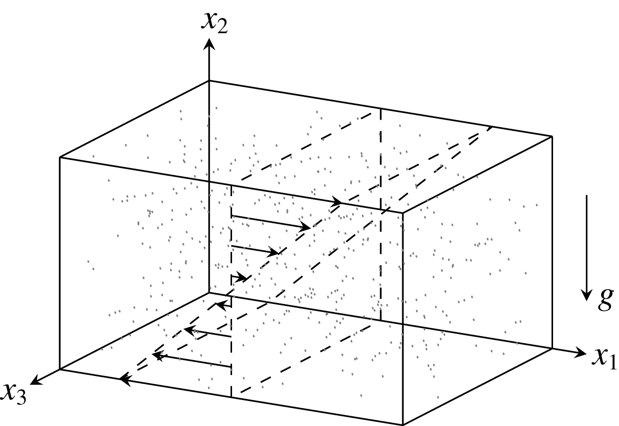
Sketch of the geometrical configuration. A background base shear
 $\unicode[STIX]{x1D6E4}x_{2}\boldsymbol{e}_{1}$
drives a turbulent gas loaded with particles. A gravitational acceleration aligned with the shear direction, i.e.
 $\boldsymbol{g}=-g\boldsymbol{e}_{2}$
, causes the particles to settle.

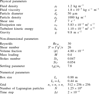
Parameters for the Euler–Lagrange simulation of homogeneously sheared turbulence.

4.2 Homogeneously sheared turbulence
The flow configuration is sketched in figure 1. The physical parameters correspond to
 $50~\unicode[STIX]{x03BC}\text{m}$
particles with density
 $\unicode[STIX]{x1D70C}_{p}=10^{3}~\text{kg}~\text{m}^{-3}$
suspended in air at the average volume fraction
 $\langle \unicode[STIX]{x1D719}\rangle =4.8\times 10^{-4}$
. At these conditions, the mass loading is
 $M=0.4$
. The flow is sheared at the rate
 $\unicode[STIX]{x1D6E4}=7~\text{s}^{-1}$
. Table 1 contains a summary of the simulation parameters.
The initial turbulence is isotropic and characterized by a Taylor micro-scale Reynolds number
 $Re_{\unicode[STIX]{x1D706},0}=30$
. The turbulent kinetic energy spectrum follows
 $$\begin{eqnarray}\displaystyle E_{0}(k)=C_{k}\unicode[STIX]{x1D716}_{0}^{2/3}\unicode[STIX]{x1D705}_{0}^{-5/3}\left\{\begin{array}{@{}ll@{}}\left(k/\unicode[STIX]{x1D705}_{0}\right)^{2}, & \quad k<\unicode[STIX]{x1D705}_{0},\\ \left(k/\unicode[STIX]{x1D705}_{0}\right)^{-5/3}, & \quad \unicode[STIX]{x1D705}_{0}\leqslant k\leqslant \unicode[STIX]{x1D705}_{\unicode[STIX]{x1D702}},\\ 0, & \quad k>\unicode[STIX]{x1D705}_{\unicode[STIX]{x1D702}},\end{array}\right. & & \displaystyle\end{eqnarray}$$
where
 $\unicode[STIX]{x1D716}_{0}$
is the initial dissipation rate,
 $\unicode[STIX]{x1D705}_{0}$
is the spectrum peak wavenumber and
 $C_{k}=1.5$
is a constant (Isaza & Collins Reference Isaza and Collins2009). The largest wavenumber
 $\unicode[STIX]{x1D705}_{\unicode[STIX]{x1D702}}$
is given by
 $$\begin{eqnarray}\unicode[STIX]{x1D705}_{\unicode[STIX]{x1D702}}=\unicode[STIX]{x1D705}_{0}\left[\frac{2\unicode[STIX]{x1D716}_{0}^{1/3}}{3\unicode[STIX]{x1D708}C_{k}\unicode[STIX]{x1D705}_{0}^{4/3}}+\frac{11}{15}\right]^{3/4}.\end{eqnarray}$$
In the present simulations, the ratio of
 $\unicode[STIX]{x1D705}_{\unicode[STIX]{x1D702}}$
to the largest wavenumber supported by the grid
 $k_{max}$
is small enough
 $\unicode[STIX]{x1D705}_{\unicode[STIX]{x1D702}}/k_{max}=0.005$
to avoid loss of resolution or confinement effects during the integration time
 $\unicode[STIX]{x1D6E4}t\leqslant 4$
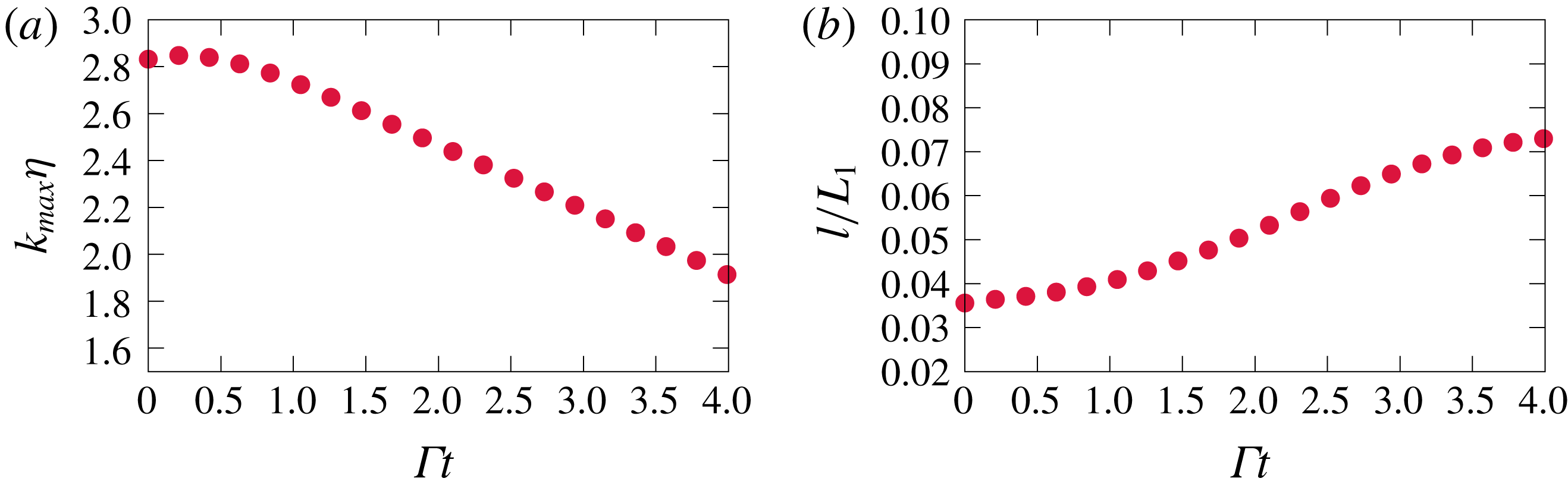
. As shown in figures 2(a) and 2(b), we maintain sufficient resolution at small scales, such that
 $k_{max}\unicode[STIX]{x1D702}\geqslant 1$
, and at large scales, such that the integral length scale
 $l\equiv \langle u_{1}^{2}\rangle ^{3/2}/\unicode[STIX]{x1D716}$
(Shen & Warhaft Reference Shen and Warhaft2000) continues growing while remaining much smaller than the box size (
 $l/L_{1}<0.08$
).
Evolution of (a) the product of the largest wavenumber resolved by the grid and the Kolmogorov scale and (b) the normalized integral length scale during the integration time
 $\unicode[STIX]{x1D6E4}t\leqslant 4$
.

The high shear number
 $S^{\ast }=26$
indicates that the shearing strongly exceeds the nonlinear inertial effects of turbulence, hence providing opportunity for comparison with RDT. The Lagrangian particles are seeded uniformly in the domain and are initialized with a velocity equal to the sum of the local fluid velocity, gravitational settling velocity and inertial correction of Ferry & Balachandar (Reference Ferry and Balachandar2001). The turbulence Stokes number
 $St_{\unicode[STIX]{x1D702}}=0.047$
and shear Stokes number
 $St_{\unicode[STIX]{x1D6E4}}=0.054$
are within the acceptable values in the present derivation of RDT.
Comparison with the theory is performed by computing the auto-correlation spectra
 $\unicode[STIX]{x1D6F7}_{i,j}$
from RDT. This quantity is defined as
 $$\begin{eqnarray}\langle f_{i}(\boldsymbol{x})f_{j}(\boldsymbol{x}+\boldsymbol{r})\rangle =\int \int \int \unicode[STIX]{x1D6F7}_{i,j}(\boldsymbol{r},t)\exp (\boldsymbol{r}\boldsymbol{\cdot }\boldsymbol{k})\,\text{d}\,\boldsymbol{k},\end{eqnarray}$$
where
 $f_{i}=u_{i}$
for
 $i=1$
to 3 and
 $f_{4}=\unicode[STIX]{x1D719}$
. In the following, we will focus on single-point statistics, namely,
 $\boldsymbol{r}=0$
. The short time expression derived in § 3.3 is used to propagate the spectra in time according to
 $$\begin{eqnarray}\unicode[STIX]{x1D6F7}_{i,j}(\boldsymbol{k},t+\unicode[STIX]{x0394}t)=\unicode[STIX]{x1D61F}_{i,p}^{\ast }(\boldsymbol{k}_{0},\unicode[STIX]{x0394}t)\unicode[STIX]{x1D61F}_{j,q}(\boldsymbol{k}_{0},\unicode[STIX]{x0394}t)\unicode[STIX]{x1D6F7}_{p,q}(\boldsymbol{k}_{0},t)+O(\unicode[STIX]{x0394}t^{2}),\end{eqnarray}$$
where
 $\boldsymbol{k}_{0}$
is any wave vector at time
 $t$
, and
 $\boldsymbol{k}$
the corresponding wave vector at
 $t+\unicode[STIX]{x0394}t$
. The initial conditions are the same as those in the simulations. At
 $t=0$
, the turbulence is homogeneous and isotropic with the spectrum (4.2), which yields the following auto-correlation spectra for the fluid velocity fluctuations
 $$\begin{eqnarray}\unicode[STIX]{x1D6F7}_{i,j}(\boldsymbol{k}_{0},0)=\frac{E(k_{0})}{4\unicode[STIX]{x03C0}k_{0}^{2}}\left(\unicode[STIX]{x1D6FF}_{ij}-\frac{k_{i,0}k_{j,0}}{k_{0}^{2}}\right),\end{eqnarray}$$
for
 $1\leqslant i\leqslant 3$
and
 $1\leqslant j\leqslant 3$
. Initially, the particles are assumed uniformly distributed and uncorrelated with the fluid, i.e.
 $$\begin{eqnarray}\displaystyle \unicode[STIX]{x1D6F7}_{4,4}(\boldsymbol{k}_{0},0) & = & \displaystyle 0,\end{eqnarray}$$
 $$\begin{eqnarray}\displaystyle \unicode[STIX]{x1D6F7}_{4,i}(\boldsymbol{k}_{0},0) & = & \displaystyle 0,\quad \text{for }1\leqslant i\leqslant 3.\end{eqnarray}$$
The quantities of interest are computed by integrating over the Fourier space. Specifically, the Reynolds stresses, volume fraction fluctuations, particle–fluid correlations and dissipation rate are obtained using
 $$\begin{eqnarray}\displaystyle & \displaystyle \langle u_{i}u_{j}\rangle =\int \int \int \unicode[STIX]{x1D6F7}_{i,j}\,\text{d}\,\boldsymbol{k},\quad 1\leqslant i,j\leqslant 3 & \displaystyle\end{eqnarray}$$
 $$\begin{eqnarray}\displaystyle & \displaystyle \langle \unicode[STIX]{x1D719}u_{i}\rangle =\int \int \int \unicode[STIX]{x1D6F7}_{4,i}\,\text{d}\,\boldsymbol{k},\quad 1\leqslant i\leqslant 3 & \displaystyle\end{eqnarray}$$
 $$\begin{eqnarray}\displaystyle & \displaystyle \langle {\unicode[STIX]{x1D719}^{\prime }}^{2}\rangle =\int \int \int \unicode[STIX]{x1D6F7}_{4,4}\,\text{d}\,\boldsymbol{k}, & \displaystyle\end{eqnarray}$$
 $$\begin{eqnarray}\displaystyle & \displaystyle \unicode[STIX]{x1D716}=\mathop{\sum }_{i=1}^{3}\int \int \int \unicode[STIX]{x1D708}k^{2}\unicode[STIX]{x1D6F7}_{i,i}\,\text{d}\,\boldsymbol{k}. & \displaystyle\end{eqnarray}$$
The triple integrals are evaluated in spherical coordinates using a mid-point rule. Notice that all initial spectra have a finite wavenumber support, considerably simplifying the numerical integration.
The simulations show a transition from an isotropic state to a highly anisotropic state within just a few
 $\unicode[STIX]{x1D6E4}t$
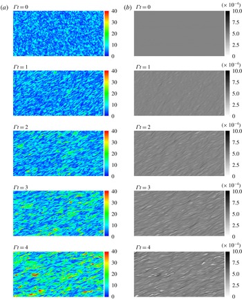
. Isocontours of the gas vorticity magnitude plotted in figure 3(a) show the stretching and tilting of vortex tubes towards the streamwise direction. This anisotropic distortion of the turbulent flow is a fundamental feature of HST. Previous work in single-phase flow HST focused on quantifying the asymptotic angle that vortex tubes make with the streamwise direction (Sukheswalla et al.
Reference Sukheswalla, Vaithianathan and Collins2013). Note that the magnitude of vorticity increases with time due to the energy injection by the mean shear flow.
Cuts in the
 $(x_{1},x_{2})$
plane of the volume fraction (b) and the vorticity magnitude, i.e.
 $\unicode[STIX]{x1D714}$
; (a) fields at consecutive times from two-way coupled Euler–Lagrange simulations.

The simulations also show the gradual accumulation of particles into elongated structures (figure 3
b). While particles are initially uniformly distributed, inhomogeneity in the particle distribution quickly emerges. By
 $\unicode[STIX]{x1D6E4}t=4$
elongated particle clusters have formed, having a volume fraction nearly twice as large as the mean volume fraction. Nearly depleted pockets develop adjacent to the particle clusters. Visual examination of figures 3(a) and 3(b) shows that the low volume fraction pockets, coincide with regions of the flow where vorticity is highest, as expected from preferential concentration. Note that the formation of clusters and void pockets is an indication of strong nonlinearities that fall out of scope of RDT. However, as we show below, the present RDT formulation explains the early stages of the clustering in HST.
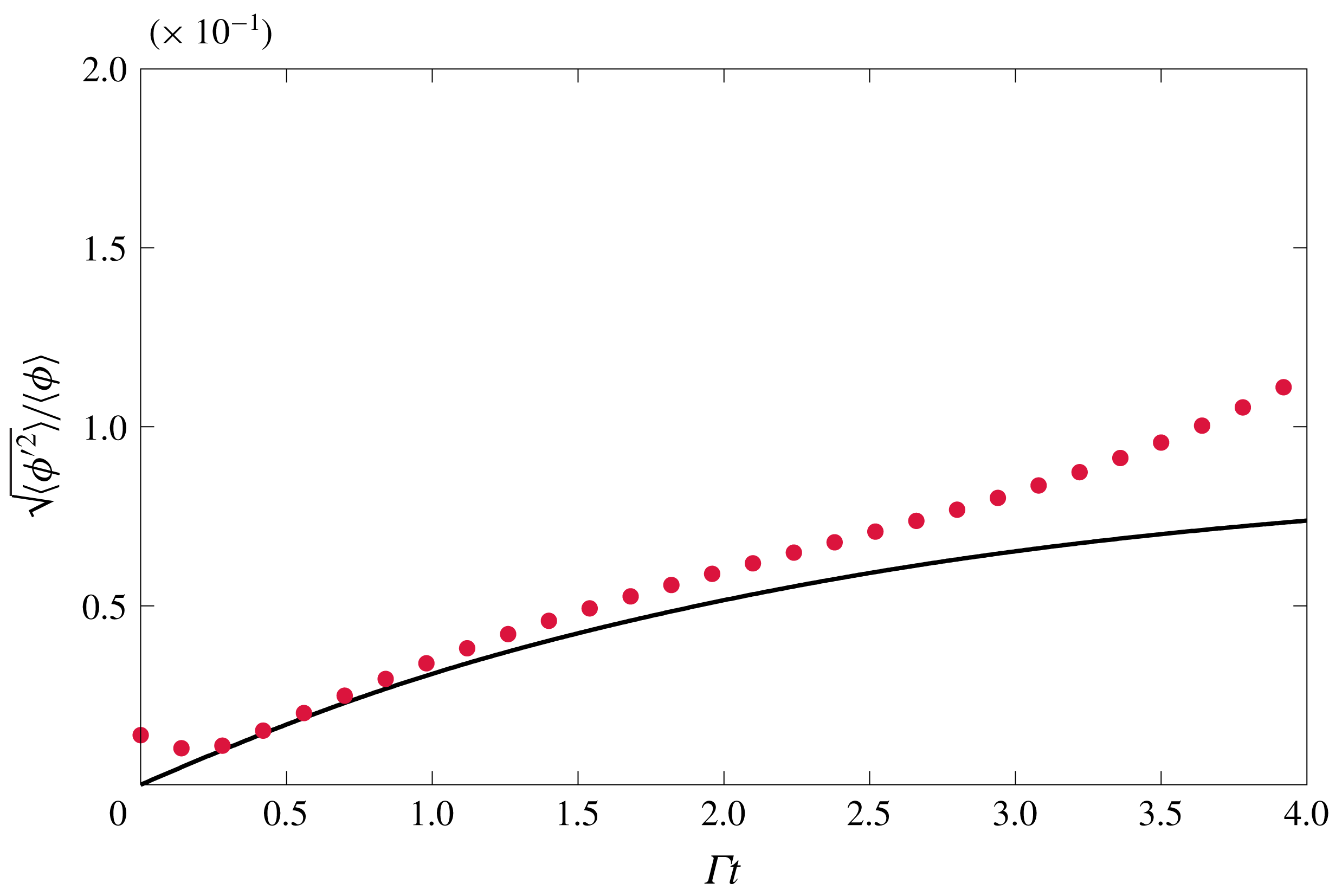
Evolution of the root mean square volume fraction fluctuations from the extended RDT (thick line) and Euler–Lagrange simulations (symbols).

As the suspension is sheared, the emergence of particle clusters is accompanied by a growth of volume fraction fluctuations. In figure 4, we report measurements from the simulations alongside values computed from RDT. Note that despite seeding the Lagrangian particles uniformly, a small volume fraction fluctuation
 $\langle \unicode[STIX]{x1D719}^{\prime 2}\rangle \neq 0$
persists due to the discrete nature of Lagrangian data. The linear theory captures the early growth of the volume fraction fluctuations within a few per cent until
 $\unicode[STIX]{x1D6E4}t\sim 0.7$
. Further, RDT shows a comparable growth rate to the simulation until
 $\unicode[STIX]{x1D6E4}t\sim 3$
. This proves that interplay between shear and preferential concentration is the main mechanism for the initiation of clusters under these conditions. Beyond
 $\unicode[STIX]{x1D6E4}t\sim 3$
, the appearance of clusters and depleted pockets in the simulations indicates a strengthening of the nonlinear mechanisms. This translates into an increase of the growth rate in the simulations compared to RDT.
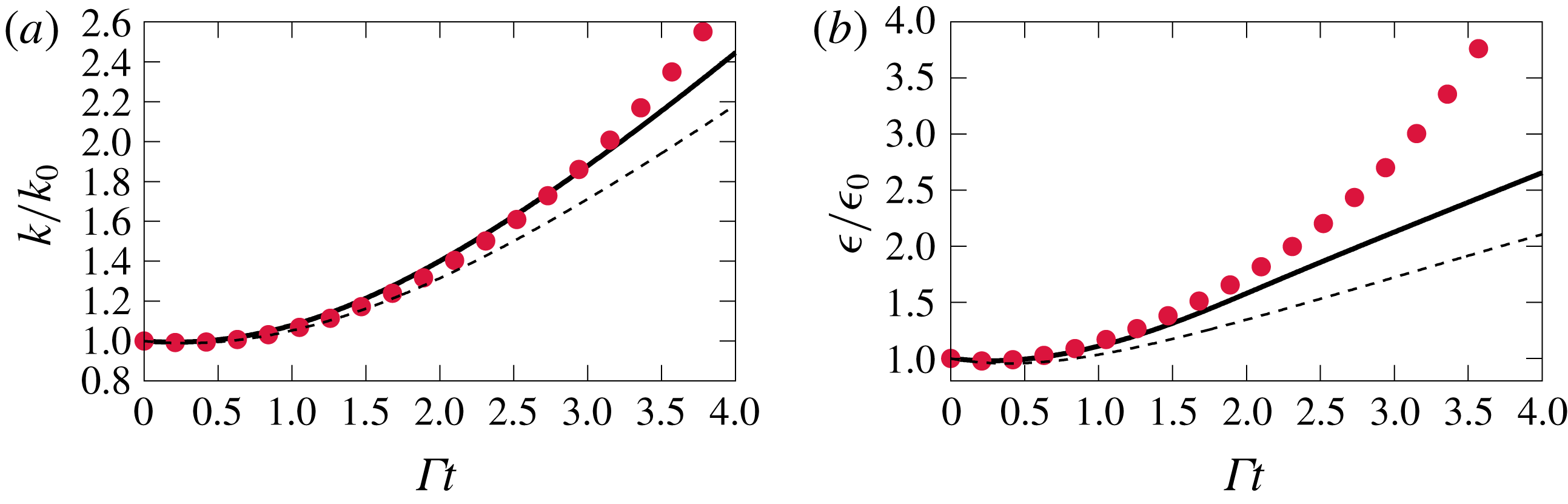
Turbulence observables computed from the extended RDT (thick lines) and Euler–Lagrange simulations (symbols). Thin lines represent results of the single-phase flow RDT (i.e.
 $\langle \unicode[STIX]{x1D719}\rangle =0$
).

The evolution of turbulent kinetic energy (TKE) and dissipation rate in the fluid phase is shown in figures 5(a) and 5(b). Rapid distortion theory captures the evolution of the TKE until
 $\unicode[STIX]{x1D6E4}t\sim 3.5$
and the dissipation rate until
 $\unicode[STIX]{x1D6E4}t\sim 2$
. The presence of particles leads to a larger growth rate of these quantities compared to the single-phase flow case. The increase in TKE is caused by the work done by gravity on the volume fraction fluctuations created by preferential concentration. Based on prior work of Elghobashi & Truesdell (Reference Elghobashi and Truesdell1992), the increase in dissipation rate can be explained by the fact that settling particles force the fast-dissipating small scale fluid motions more than large scales. This is also in agreement with our previous work (Kasbaoui et al.
Reference Kasbaoui, Koch, Subramanian and Desjardins2015), where we showed that the largest velocity fluctuations induced by the combined action of preferential concentration and shear have a length scale controlled by viscous dissipation that expresses as
 $$\begin{eqnarray}\sqrt{\unicode[STIX]{x1D708}/\unicode[STIX]{x1D6E4}}=\unicode[STIX]{x1D702}/\sqrt{\unicode[STIX]{x1D6E4}\unicode[STIX]{x1D70F}_{\unicode[STIX]{x1D702}}}=\unicode[STIX]{x1D702}\sqrt{St_{\unicode[STIX]{x1D702}}/St_{\unicode[STIX]{x1D6E4}}}\sim \unicode[STIX]{x1D702}.\end{eqnarray}$$
Therefore, these fluctuations contribute primarily to the increase of the dissipation rate. Beyond
 $\unicode[STIX]{x1D6E4}t\sim 2$
, nonlinear effects lead to growth rates of the TKE and dissipation rate higher than those predicted by the linear theory.
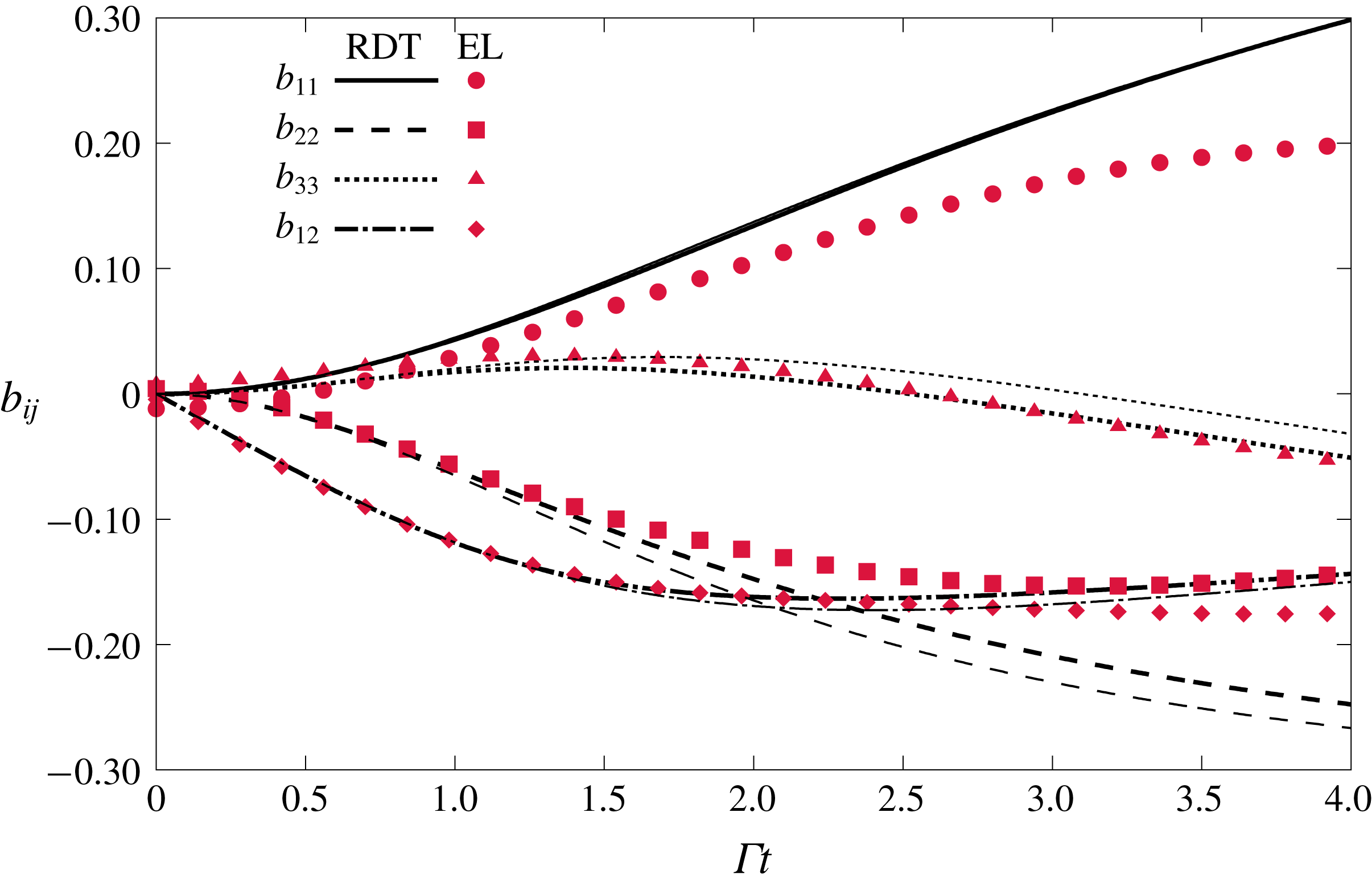
Anisotropic Reynolds stresses computed from the extended RDT (thick lines) and Euler–Lagrange (EL) simulations (symbols). Thin dashed lines represent results of the single-phase flow RDT (i.e.
 $\langle \unicode[STIX]{x1D719}\rangle =0$
).

In addition to the modulation of the TKE and dissipation rate, the suspended particles modify the anisotropic structures in HST. We quantify the directional anisotropy with an analysis of the anisotropic Reynolds stresses
 $b_{ij}=\langle u_{i}u_{j}\rangle /2k-\unicode[STIX]{x1D6FF}_{ij}/3$
(see figure 6). In the present case, the particle-laden flow RDT shows good agreement with the simulations until
 $\unicode[STIX]{x1D6E4}t\sim 2$
. Compared to the unladen case (
 $\langle \unicode[STIX]{x1D719}\rangle =0$
), the extended RDT predicts an increase of component
 $b_{22}$
which is also seen in the simulations. This is expected since the gravitational loading particles exert on the gas drives fluctuations in the gravity direction
 $x_{2}$
. The accumulation of kinetic energy in the streamwise and settling directions reduces the proportion of kinetic energy in the spanwise direction. This manifests as a lower
 $b_{33}$
component in the extended RDT and Euler–Lagrange simulations. Note that in single phase HST at
 $\unicode[STIX]{x1D6E4}t=4$
, the value of
 $b_{22}$
approaching
 $-1/3$
suggests that the flow is made of loosely correlated (small
 $b_{12}$
) two-dimensional turbulence slices in the
 $x_{1}$
–
 $x_{3}$
plane. The forcing that particles exert on the gas opposes this distortion of turbulence as manifested by an increase of
 $b_{12}$
,
 $b_{22}$
and lowering of
 $b_{33}$
. Further, in the simulations,
 $b_{11}$
is lowered, suggesting a weaker action of shear along the streamwise direction. Overall, Euler–Lagrange simulations show a lower degree of anisotropy than RDT likely due to strong nonlinear processes.
5 Conclusion
In this paper, we laid the foundation for the analysis of homogeneously sheared particle-laden turbulence in the two-way coupled semi-dilute regime using rapid distortion theory. The analysis presented relies on two assumptions: (i) the particles are small enough to have small but non-zero inertia, and (ii) the shearing happens on a time scale faster than the integral time scale of the turbulence. The approach allows the description of the turbulence spectral content in a semi-analytical form. It is shown that, in addition to the distortion by the shear, the Fourier modes are further altered due to the preferential concentration mechanism and the gravitational loading exerted by the particles.
The application of RDT to particle-laden HST provides semi-analytical expressions for the turbulent velocity and volume fraction fluctuations. These forms can be used to compute the evolution of various turbulence statistics such as the turbulent kinetic energy and volume fraction variance. For the various quantities measured, we show that there is a quantitative agreement until
 $\unicode[STIX]{x1D6E4}t\sim 1$
between the extended RDT and Euler–Lagrange simulations. Most notably, the linear theory is able to predict the initial growth of the root mean square of volume fraction fluctuations. Remarkably, the simulations show the formation of clusters and depleted pockets within a few
 $\unicode[STIX]{x1D6E4}t$
even for the small Stokes number considered (
 $St_{\unicode[STIX]{x1D702}}=0.047$
,
 $St_{\unicode[STIX]{x1D6E4}}=0.54$
). While these latter effects are inherently nonlinear, the ability of RDT to capture the initial growth of volume fraction fluctuations confirms that clustering in the semi-dilute regime is triggered by an interplay between shear and preferential concentration.
Further analysis of particle-laden HST, shows a modulation of the anisotropic stresses in both Euler–Lagrange simulations and RDT. We found that the coupling between the particulate phase and the fluid enhances the turbulent kinetic energy and dissipation rate, and causes a change of the turbulence organization in a way that opposes the anisotropic distortion caused by the shear. However, this modulation, while qualitatively captured by RDT, is stronger in the simulations at large
 $\unicode[STIX]{x1D6E4}t$
due to nonlinear mechanisms such as clustering, and nonlinear inertial effects.
Acknowledgements
This work was supported by NSF grants CBET-1233793, CBET-1505759 and CBET-1437903.
Appendix A. Short time approximation of the rapid distortion matrix
Due to the challenges in integrating analytically equation (3.23), we focus here on providing a short time approximation of operator
 $\unicode[STIX]{x1D650}$
. The goal is to build a numerical integrator that can propagate the solution forward in time. Various approaches can be used to build an approximate solution, including the Magnus expansion which can provide high-order approximations of the analytical exponential solution (Magnus Reference Magnus1954; Blanes et al.
Reference Blanes, Casas, Oteo and Ros2009; Duran & Moreau Reference Duran and Moreau2013). To keep the derivation simple, we use an explicit Euler scheme (first order) to approximate
 $\unicode[STIX]{x1D650}$
at
 $\unicode[STIX]{x0394}t$
 $$\begin{eqnarray}\displaystyle \unicode[STIX]{x1D650}(\unicode[STIX]{x0394}t) & = & \displaystyle \unicode[STIX]{x1D650}(0)-\unicode[STIX]{x0394}t\unicode[STIX]{x1D63E}^{\prime }\unicode[STIX]{x1D650}(0)+O(\unicode[STIX]{x0394}t^{2})\end{eqnarray}$$
 $$\begin{eqnarray}\displaystyle & = & \displaystyle \unicode[STIX]{x1D644}-\unicode[STIX]{x0394}t\unicode[STIX]{x1D63E}(0)+O(\unicode[STIX]{x0394}t^{2}).\end{eqnarray}$$
Since the RDT operator is
 $\unicode[STIX]{x1D653}=\unicode[STIX]{x1D63C}\unicode[STIX]{x1D654}\unicode[STIX]{x1D655}\unicode[STIX]{x1D650}$
, this leads to the following approximation
 $$\begin{eqnarray}\displaystyle \unicode[STIX]{x1D653}(\unicode[STIX]{x0394}t) & = & \displaystyle \unicode[STIX]{x1D63C}(\unicode[STIX]{x0394}t)\unicode[STIX]{x1D654}(\unicode[STIX]{x0394}t)\unicode[STIX]{x1D655}(\unicode[STIX]{x0394}t)\unicode[STIX]{x1D650}(\unicode[STIX]{x0394}t)\end{eqnarray}$$
 $$\begin{eqnarray}\displaystyle & = & \displaystyle \unicode[STIX]{x1D63C}(\unicode[STIX]{x0394}t)\unicode[STIX]{x1D654}(\unicode[STIX]{x0394}t)\unicode[STIX]{x1D655}(\unicode[STIX]{x0394}t)\left(\unicode[STIX]{x1D644}-\unicode[STIX]{x0394}t\unicode[STIX]{x1D63E}(0)\right)+O(\unicode[STIX]{x0394}t^{2}).\end{eqnarray}$$
This leads to the following operator
 $$\begin{eqnarray}\displaystyle & \displaystyle \unicode[STIX]{x1D653}(\boldsymbol{k}_{0},\unicode[STIX]{x0394}t)=\left(\begin{array}{@{}llll@{}}\text{e}^{-\unicode[STIX]{x1D6EC}_{1}} & \text{e}^{-\unicode[STIX]{x1D6EC}_{1}}a_{12} & 0 & -\unicode[STIX]{x0394}t\text{e}^{-\unicode[STIX]{x1D6EC}_{1}}(c_{14}+a_{12}c_{24})\\ 0 & \text{e}^{-\unicode[STIX]{x1D6EC}_{1}}a_{22} & 0 & -\unicode[STIX]{x0394}t\text{e}^{-\unicode[STIX]{x1D6EC}_{1}}c_{24}a_{22}\\ 0 & \text{e}^{-\unicode[STIX]{x1D6EC}_{1}}a_{32} & \text{e}^{-\unicode[STIX]{x1D6EC}_{1}} & -\unicode[STIX]{x0394}t\text{e}^{-\unicode[STIX]{x1D6EC}_{1}}(c_{34}+a_{32}c_{24})\\ 0 & -\unicode[STIX]{x0394}t\text{e}^{-\unicode[STIX]{x1D6EC}_{2}}c_{42} & 0 & \text{e}^{-\unicode[STIX]{x1D6EC}_{2}}\end{array}\right) & \displaystyle\end{eqnarray}$$
 $$\begin{eqnarray}\displaystyle & \displaystyle \unicode[STIX]{x1D6EC}_{1}=\unicode[STIX]{x0394}t\frac{\unicode[STIX]{x1D707}_{f}}{\unicode[STIX]{x1D70C}_{m}}\left(k_{0}^{2}-k_{1,0}k_{2,0}\unicode[STIX]{x1D6E4}\unicode[STIX]{x0394}t+\frac{(k_{1,0}\unicode[STIX]{x1D6E4}\unicode[STIX]{x0394}t)^{2}}{3}\right)\quad & \displaystyle \nonumber\\ \displaystyle & \displaystyle +\,\frac{\unicode[STIX]{x1D70C}_{p}\langle \unicode[STIX]{x1D719}\rangle }{\unicode[STIX]{x1D70C}_{m}}\text{i}\unicode[STIX]{x0394}t\left(\unicode[STIX]{x1D650}_{g}\boldsymbol{\cdot }\boldsymbol{k}_{0}-U_{g,2}\unicode[STIX]{x1D6E4}\unicode[STIX]{x0394}t\frac{k_{1}}{2}\right), & \displaystyle\end{eqnarray}$$
 $$\begin{eqnarray}\displaystyle & \displaystyle \unicode[STIX]{x1D6EC}_{2}=\text{i}\unicode[STIX]{x0394}t\left(\unicode[STIX]{x1D650}_{g}\boldsymbol{\cdot }\boldsymbol{k}_{0}-U_{g,2}\unicode[STIX]{x1D6E4}\unicode[STIX]{x0394}t\frac{k_{1}}{2}\right). & \displaystyle\end{eqnarray}$$
The fluctuating quantities evolve from
 $t$
to
 $t+\unicode[STIX]{x0394}t$
according to
 $$\begin{eqnarray}\displaystyle \unicode[STIX]{x1D712}(t+\unicode[STIX]{x0394}t)=\unicode[STIX]{x1D653}(\unicode[STIX]{x0394}t)\unicode[STIX]{x1D712}(t)+O(\unicode[STIX]{x0394}t^{2}). & & \displaystyle\end{eqnarray}$$