
1. State of the art
In 2020, the number of objects launched into space was three times higher than in 2019, due exclusively to commercial activities (ESOC 2021). As the number of objects orbiting the Earth continues to increase, the issue of debris, and consequently debris re-entering the atmosphere, can no longer be dismissed. Moreover, the damage generated by large pieces of debris could be dramatic if the objects reach populated areas (Ailor & Patera Reference Ailor and Patera2007). In order to prevent these kinds of negative consequences, various types of studies are being done. Some researchers are developing innovative systems to capture debris before it enters the atmosphere, thereby preserving the active space stations (Flores-Abad et al. Reference Flores-Abad, Ma, Pham and Ulrich2014; More & Murugan Reference More and Murugan2021). Other studies focus on improving the predictive impact time and area, including estimation of the debris dispersion (Reyhanoglu & Alvarado Reference Reyhanoglu and Alvarado2013). Nevertheless, we are still poorly informed about some debris properties, such as the initial state vector, the ambient atmospheric conditions and key parameters, including the ballistic coefficients. The work on the observation of space debris (Hossein et al. Reference Hossein, Acernese, Cardona, Cialone, Curianò, Mariani, Marini, Marzioli, Parisi and Piergentili2020) has provided information on breakup events (Lips Reference Lips2003), while fragments from the destruction of space vehicles surviving to the ground have been analysed in order to study how they impacted the Earth (Park & Park Reference Park and Park2017), as in the tragic accident of the Colombia shuttle (Ailor et al. Reference Ailor, Hallman, Steckel and Weaver2005) or the re-entry of the Chinese space station Tiangong-1 (Ahmad & Fitri Reference Ahmad and Fitri2021). These data may help to build breakup scenarios and improve the predictive capabilities of re-entry debris codes.
Nowadays, atmospheric re-entry trajectory and survivability predictive codes are being developed by research centres and space agencies. The available codes can be classified into two main categories: object-oriented codes and spacecraft-oriented codes Lips & Fritsche (Reference Lips and Fritsche2005). The object-oriented method is based on simplifying the complicated geometry of objects into simple shapes such as sphere, cylinder, box, etc. Tools using this method are DAS, ORSAT and DRAPS. In particular, ORSAT, developed by NASA, also includes thermal/ablation models to determine the debris survivability assessment (Ostrom & Sanchez Reference Ostrom and Sanchez2018). The ESA with SCARAB has opted for the spacecraft-oriented method to simulate the re-entry of spacecraft in as real a way as possible; nevertheless, due to a much more complex analysis strategy, this method requires great modelling efforts and computing resources (Lips et al. Reference Lips, Fritsche, Koppenwallner and Klinkrad2004; Koppenwallner et al. Reference Koppenwallner, Fritsche, Lips and Heiner2005). PAMPERO developed by the CNES agency since 2013 is another predictive code based on spacecraft-oriented tools (Annaloro et al. Reference Annaloro, Galera, Kärräng, Prigent, Lips and Omaly2017).
The determination of destructive re-entries and the prediction of the potential for ground risk due to the arrival of fragmented objects on the ground are the main purposes of these numerical codes. The breakup is estimated to occur at altitudes between 90 and 65 km (Kärräng, Lips & Soares Reference Kärräng, Lips and Soares2019) and is the consequence of strong external forces leading generally to the fragmentation of the debris (Prevereaud et al. Reference Prevereaud, Vérant, Moschetta, Sourgen and Blanchard2012; Lips Reference Lips2013; Park et al. Reference Park, Laboulais, Leyland and Mischler2020). As a result, one large object becomes a multitude of smaller ones that will interact with each other. These interactions exist at least in the first moments after fragmentation, where the flow is still rarefied. Note that nowadays, this flow regime still needs to be better explored. As evidence, bridging functions describing aero-thermodynamics coefficients, that take into account the different flow regimes involved, are used to improve trajectory predictions and the demise of debris (Park et al. Reference Park, Laboulais, Leyland and Mischler2020). Atmospheric re-entry can lead to different behaviour of the debris’ flight depending on its size, shape and material. Evolving at hypersonic velocities, debris entering the atmosphere penetrates an increasingly dense medium as its altitude decreases. Thus it undergoes successively four different flow regimes: free-molecular, transition, slip-flow and continuum. Approaching the Earth, the dynamic pressure and heat flux increase. Most of the time, a small object does not survive this phase, but a larger one can, at least partially, hit the Earth. Different scenarios can occur leading to a longer preservation of the following debris, or to its accelerated destruction. In any case, the interactions between pieces of debris lead to a change in their trajectories, which increases the difficulty of predicting ground impacts (Ahmad & Fitri Reference Ahmad and Fitri2021). These difficulties are mainly due to viscous effects that have to be taken into account when analysing and describing shock/shock interactions. They concern not only 1 m diameter objects flying at hypersonic speeds, but also smaller parts that are manufactured at high melting temperatures (Koppenwallner, Fritsche & Lips Reference Koppenwallner, Fritsche and Lips2001).
Therefore, the topic of proximal bodies is of great interest. The aim of this experimental work is to study how rarefaction and viscous effects could modify the aero-thermodynamic properties of shock/shock interactions. Our motivation is to bring new knowledge to improve the prediction of the fate of objects entering the Earth's atmosphere. This study is not restrictive to this application and can also be useful for other scenarios concerning high speed combined with high altitude of an atmospheric re-entry.
Many studies concerning the interaction of objects focused on the study of Edney's shock/shock interferences (Edney Reference Edney1968), since they play a major role in the aero-thermodynamics observed behaviours. Numerous experimental and theoretical studies investigated interferences between an oblique shock generated by a wedge and a bow shock, most often produced by a cylinder. These works were motivated by high local heating rates at hypersonic speeds occurring in critical situations, such as shock/shock interferences on a deflected flap, along axial corners in wing–body or on fin–wing junctions. Shock-wave/boundary-layer interactions also occur in air-intakes of breathing propulsive systems. Such interactions can induce separation of the boundary layer, which causes loss in control effectiveness in the engine inlet, with the subsequent reattachment of the separated shear layer giving rise to heat-transfer rates. Many studies have focused on Edney type IV interactions as this is the most critical shock–impact interaction in terms of aero-thermal loads at the wall. Most studies have been carried out experimentally in shock tubes or numerically with a computational fluid dynamics approach, in the continuum regime (Sanderson Reference Sanderson1995; Windisch, Reinartz & Müller Reference Windisch, Reinartz and Müller2016; Khatta & Gopalan Reference Khatta and Gopalan2018; Paoli Reference Paoli2018). Only a few authors have shown interest in studying the influence of viscous effects on the thermal effects of Edney type IV interactions, and have shown a decrease in heat loads in the slip regime (Carlson & Wilmoth Reference Carlson and Wilmoth1992; Glass Reference Glass1999; Moss et al. Reference Moss, Pot, Chanetz and Lefebvre1999; Pot et al. Reference Pot, Chanetz, Lefebvre and Bouchardy1999; Riabov & Botin Reference Riabov and Botin1999; Grasso et al. Reference Grasso, Purpura, Chanetz and Délery2003; Lu et al. Reference Lu, Yue, Xiao and Zhang2013).
Regarding the specific subject of space debris re-entry, the geometries of the objects concerned have a closed geometry (spheres, cylinders, cubes, plates) that will form bow shocks. In this context, more recent work has been carried out to study more specifically bow shock interactions, experimentally always in a continuum regime, and numerically in continuum and rarefied regimes (Vashchenkov, Kashkovsky & Ivanov Reference Vashchenkov, Kashkovsky and Ivanov2003). Some major works investigated interactions between two or several spheres. Indeed, the sphere–sphere case is a canonical geometry that can nevertheless be expected to exhibit many of the important flow features of more realistic geometries. The trajectories of the interacting spheres were analysed experimentally in shock tube facilities using the free flight method (Laurence, Deiterding & Hornung Reference Laurence, Deiterding and Hornung2007; Laurence, Parziale & Deiterding Reference Laurence, Parziale and Deiterding2012; Park & Brown Reference Park and Brown2012; Fisher, Quinn & Smith Reference Fisher, Quinn and Smith2018; Marwege et al. Reference Marwege, Willems, Gülhan, Aftosmis and Stern2018; Whalen & Laurence Reference Whalen and Laurence2021). Only one experimental work concerns the interaction of cylinders in free flight conditions with a hypersonic shock tube (Leiser et al. Reference Leiser, Löhle, Zander, Buttsworth, Choudhury and Fasoulas2022).
The literature shows that studies of the bow shock interaction have so far been conducted in the continuum regime and do not take into account the viscous effects that can occur due to high velocities and low atmospheric density. This experimental work focuses on the study of the interaction between two spheres in a low pressure supersonic flow in the slip regime, representative of an altitude of 76 km. Experiments have been carried out with flow conditions of Mach 4 and ambient pressure 2.67 Pa. Previous work by Cardona, Joussot & Lago (Reference Cardona, Joussot and Lago2021) has shown that the different types of Edney interference can be identified; however, some differences appear with respect to the continuous regime, such as the thickening of the shock and the boundary layer, which leads to the vanishing of the impinging jets that appear in type IV interference. This study goes further and analyses the impact of the viscous effects on the rear sphere in the wake of the first one. In order to simplify this study, it has been chosen to have both spheres of the same diameter. Different diagnostics have been applied in order to analyse the impact of low density on different parameters that influence the aero-thermodynamics of interacting spheres. Shock/shock interferences will be analysed in terms of shock-wave shapes, drag and lift forces, and wall pressure distribution of the second sphere. To complete the study, a pendulum method was adopted to characterize the wake of a sphere in a supersonic rarefied flow. This non-intrusive method will also be used to evaluate the effect of the second sphere on the first one. This experimental work allows the analysis of the influence of viscous effects on the different parameters that are affected by the shock/shock interactions, and of which physical properties are the most affected. In addition, this dataset will allow the validation and improvement of certain physical models, in particular those concerning the aerodynamics used in the debris entry prediction codes. To our knowledge, no experiments have been conducted with two spheres interacting in a rarefied flow. This topic seems to have been exclusively studied experimentally and numerically in a continuum regime, and numerically in a rarefied flow. Still, some parameters are poorly explored, such as the distribution of pressure or heat transfer at the surface of the second sphere. No full study has yet been conducted to link aerodynamic properties with surface parameters such as wall pressure. Numerically, even if calculations representative of rarefied flows are improving, some questions still need to be addressed, in particular, the determination of accommodation coefficients (Zuppardi & Paterna Reference Zuppardi and Paterna2015). These parameters originate in slip conditions, thus in the boundary layer of an object. In a rarefied flow, the physics is still poorly understood, which is why some experimental data can provide important information.
2. Experimental conditions
2.1. MARHy wind tunnel
The experiments presented in this paper were carried out in the MARHy wind tunnel, one of the three wind tunnels of the FAST platform at ICARE, CNRS (France). MARHy is a rarefied wind tunnel that can create flow from Mach 0.8 up to Mach 20, thanks to the 23 interchangeable nozzles that can generate different low-density flows representative of the early stages of space flight or atmospheric re-entry.
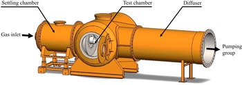
As shown in figure 1, the wind tunnel is composed of three main parts: the settling chamber, the test chamber and the diffuser. The first part is used to establish the stagnation conditions of the flow. The air flow entering the chamber, and hence the static pressure in the settling chamber, are regulated by a gas valve. The air is then accelerated through the chosen nozzle and expands into the test chamber. There, the free-stream conditions depend on the stagnation conditions, the nozzle and the pumping conditions. The third part, the diffuser, links the test chamber to the pumping group, which is composed of two primary type pumps and 14 Roots blowers. The pumping group is able to keep operating conditions in a stable and continuous mode, with no time limit.
Schematic view of the MARHy wind tunnel.

Depending on the nozzle used during experiments, the flow can reach a large range of speeds and pressures. For Mach numbers below 5, the test gas is ambient air, which was the case for the set of experiments presented in this paper. For hypersonic flows, the test gas used is dinitrogen. Regardless of the nozzle used, the flow is laminar and continuous in the isotropic core thanks to the stable stagnation conditions and the powerful pumping group. The diameter and length of the isotropic core, where the free-stream conditions are well known, depend on the nozzle used.
Stagnation and free-stream conditions are obtained by adjusting, respectively, the pressures in the settling chamber and in the test chamber independently (see figure 1). The stagnation pressure is regulated and stabilized accurately with a micro-valve placed at the inlet of the settling chamber. The free-stream pressure in the test chamber is regulated by commissioning the right number of Roots blowers, and is adjusted by opening the butterfly valve placed between the diffuser and the pumping group. Pressures are monitored with MKS absolute pressure sensors. Their full range is chosen to be in accordance with expected values: a 10 torr sensor for the stagnation pressure ( $p_o$), and 0.1 torr for the free-stream pressure (
 $p_\infty$), respectively accurate to 0.12 % and 0.15 % of reading. The control of static and infinite upstream flow pressures ensures stable flow conditions in terms of velocity and density. Given the accuracy of the sensors, the maximum Mach number deviation is 2.6 %.
2.2. Flow conditions
The purpose of this work was to investigate the interaction of two spherical fragments of debris when re-entering the atmosphere in the upper layers, where the flow regime is rarefied. For the study to be representative of the flow properties of space debris, experimental conditions have to recreate a level of rarefaction equivalent to that at breakup altitude. The rarefaction level is characterized with the mean free path,  $\lambda _{\infty }$, defined as the distance between two collisions of molecules. Assuming the variable cross-section hard sphere model, this parameter can be calculated with (2.1) (Bird Reference Bird1994), where
 $\omega _\infty$ is given by the viscosity power law of Sutherland. For the chosen nozzle (Mach 4, 2.67 Pa), whose experimental conditions are presented in table 1,
 $\omega _\infty =0.92$ (see Appendix C, table 3) and
 \begin{equation} \lambda_{\infty} = \frac{\mu_{\infty}}{\rho_{\infty} \sqrt{2 R_m T_\infty}}\,\frac{2 (7-2 \omega_\infty) (5-2 \omega_\infty)}{15 \sqrt{\rm \pi}}. \end{equation}
Flow conditions of the Mach 4, 2.67 Pa nozzle.

To evaluate the type of flow regime in terms of collisions, very often the free-stream Knudsen number  $Kn_\infty$ (see (2.2)) is used to compare the size of the considered object with respect to the mean free path. In the present study the diameter of the first sphere
 $D_1$ is considered as the reference distance to determine the global Knudsen number:
 \begin{equation} Kn_{\infty}= \frac{\lambda_{\infty}}{D_1}. \end{equation}
Considering an estimated fragmentation altitude between 91 and 50 km, the MSISE-90 model gives a free-stream pressure ranging between 0.1 and 100 Pa, and a mean free path ranging between  $3.10^{-2}$ and
 $7.10^{-5}$ m. Ground test experimental simulation of the complete physical conditions of the atmospheric entry of space debris is extremely hard, and there is no facility able to reproduce such conditions. Nevertheless, the study of an analogous rarefaction effect is possible in wind tunnels since another similitude parameter may be used to take into consideration high-speed velocities, namely the similarity number (Chambre & Schaaf Reference Chambre and Schaaf1961; Wuest Reference Wuest1974; Macrossan Reference Macrossan2007), described with
 \begin{equation} \varsigma = \frac{Ma_{\infty}}{\sqrt{Re_{\infty}}}. \end{equation}
As can be seen, this parameter is based on the appropriate Mach and Reynolds numbers, taking into account dynamic and viscosity effects. As discussed in Cardona et al. (Reference Cardona, Joussot and Lago2021), the chosen models (see § 2.3) and nozzle give  $\varsigma =0.233$ and
 $Kn_\infty =0.0139$. When considering the similarity parameter, experimental conditions are representative of a 1 m diameter main debris fragmenting at 76 km in altitude, according to the MSISE-90 atmospheric model and the velocities given in Prevereaud et al. (Reference Prevereaud, Vérant, Moschetta, Sourgen and Blanchard2012). Consequently, free-stream experimental conditions are coherent with the expected level of rarefaction at fragmentation altitudes.
2.3. Models and general configuration of the set-up
The experiments presented in this paper were carried out in the MARHy wind tunnel described above, equipped with the nozzle detailed in table 1.
Two spheres were used as experimental models that act as blunt bodies that represent a large variety of debris shapes. The first sphere,  $S_1$, represents the parent debris, and the second sphere,
 $S_2$, a debris fragment detached from
 $S_1$. The spheres are made of Polyoxymethylene (POM), painted with thin black spray paint to increase contrast and improve image analysis. Painted, they both have same size (16 mm diameter) and mass (2.88 g with the paint). The choice of the diameter of the spheres was motivated by different reasons: the spheres must be large enough to be instrumented and also to allow an accurate visualization of the flow around them; but at the same time, they must not be too large to ensure that the shock of the two spheres can always be contained in the useful core of the flow whatever the relative position of the two spheres.
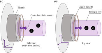
As described schematically in figure 2, the axes of symmetry of the two spheres are aligned with the vertical plane  $Y=0$ passing through the axis of symmetry of the nozzle. The experiment consists in moving the second sphere vertically, leaving the first one fixed, in order to analyse the physical properties of the interaction of the shocks produced by the two spheres. The outside diameter of the divergent nozzle is 220 mm, but the isentropic flow core is only 75 mm in diameter. In order to have enough clearance to move sphere
 $S_2$, the centre of
 $S_1$ is placed at
 $Z=-30$ mm. As presented in Cardona et al. (Reference Cardona, Joussot and Lago2021), this position does not significantly alter the free-stream flow seen by
 $S_1$, or its shock-wave shape. Moreover, since the point of interest is the effect of shock/shock interferences, if
 $S_1$ is always at the same position in the flow, then even a slight modification in its shock waves will not impact our study much. The second sphere will be moved to many different positions behind
 $S_1$ in the
 $\boldsymbol {x}$ and
 $\boldsymbol {z}$ axes. Throughout this work, the stagnation point of
 $S_1$ is taken as the origin of the spatial reference, and the axes
 $\boldsymbol {x}$,
 $\boldsymbol {y}$ and
 $\boldsymbol {z}$ are oriented as shown in figure 2. Here,
 $(X_2,Z_2)$ are the coordinates of the nose of
 $S_2$ in this spatial reference. More details concerning the different set-ups will be given in § 3.
General configuration of the set-up.

3. Experimental devices and post-processing
3.1. Flow-field visualization
3.1.1. Set-up
To visualize the flow field, the two spheres are held in position with profiled supports, which do not obstruct the flow. Sphere  $S_1$ is maintained with a vertical support fixed in a rotary system to allow the sphere to be removed from the flow in order to record background images. Sphere
 $S_2$ is maintained with a horizontal support coming from the rear of the sphere so as not to be intrusive. This support is fixed on a triaxial displacement system so that
 $S_2$ can be moved in the wake of
 $S_1$, and also removed from the flow for the recording of background images.
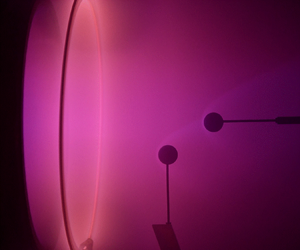
The low density of current experimental conditions does not allow the application of common techniques such as schlieren or particle image velocimetry to visualize and analyse the flow field. A technique used less commonly but adapted to our experimental conditions is used in this work. It is the technique of the glow discharge based on a cathode to ionize molecules. In our experiment, the cathode was made of copper and was placed upstream of the models around the exit of the nozzle, as shown in figure 2. It consists in applying an electrical discharge on a cathode placed near the flow. A negative voltage  $-$1 kV is applied on the copper ring, inducing current 4 mA. The polarization is low enough not to modify the nature of the flow (Coumar & Lago Reference Coumar and Lago2017). With this method, a local increase in density induces an increase in the local emitted luminous intensity. Since a shock wave is a compression of molecules, the glow discharge makes it possible to determine visually the shock waves of the spheres, by analysing the brighter region.
This method generates a volumetric illumination of the flow. Consequently, all the images taken are the result of luminous integration in the line of sight of the eye or of any recording tool. So even if the glow discharge technique can determine shock waves, the local density cannot be calculated with a simple scaling law.
Images were recorded with a Kuro CMOS camera using back illumination. The camera is equipped with a VUV objective lens that gives a resolution 154  $\mathrm {\mu }$m px
 $^{-1}$. For each relative positioning of the spheres (
 $S_1$ and
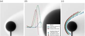
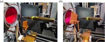
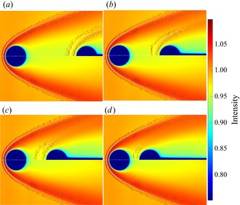
 $S_2$ fixed during acquisition), a set of 200 raw images was recorded, with exposure time 60 ms. An equivalent set of images without the models in the flow was recorded as background image. For each position, images of the flow are averaged and divided by the mean background image. This processing allows us to reduce the noise of images and avoid luminous gradient due to the experimental set-up. The resulting normalized image, shown in figure 3(a), presents an improved luminous contrast of images that allows the analysis of shock waves.
Detection of a sphere thick shock wave. (a) Normalised image of the flow around a single sphere; (b) detection method on a pixel line; (c) result of shock-wave detection on the entire image.

3.1.2. Shock-wave detection
Images give important information, in particular, on shock-wave shapes. In our study, the detection of shock waves is a key step to determine the type of shock/shock interferences that occur. This detection is based on the luminous intensity of the images. Kovacs et al. (Reference Kovacs, Passaggia, Mazellier and Lago2022) proposed the Fourier self-deconvolution (FSD) method, which was developed and validated for our specific experimental conditions. This method is applied to the present work. As illustrated in figure 3(b), the luminous intensity in analysed for each horizontal line of pixels, and allows us to define three regions due to the thickness of the shock wave: the maximal intensity, the FSD maximum, and the maximum of the FSD derivative. In what follows, the three regions will be named, from upstream to the surface of the sphere, as: foot of shock (FS), middle of shock (MS), and boundary layer (BL). Concerning this last region, the maximum luminosity is representative of the denser region. Close to the surface of the sphere, particularly at the front half, this denser region corresponds to the boundary layer. Outside this area, this term of BL is inappropriate. However, it will be more convenient to call it BL in the rest of this paper. Note that the region between the FS and the BL is called ‘middle’ but obviously, it is not located at the centre. Applying the method on each horizontal line of pixels of the image, we obtain three well-plotted regions corresponding to the regions described previously, as shown in figure 3(c).
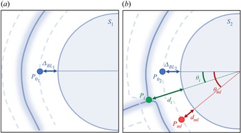
The analysis of the images, and more specifically the intensity values, can also provide important information to locate regions of stronger interactions. Figure 4 shows the four main points that will be used to deepen the knowledge on the effect of shock/shock interferences in supersonic rarefied flows. Thanks to the shock-wave detection, the intersection point  $P_i$ between the middle shock of the two spheres is found, where
 $P_i$ is characterized by
 $d_i$ and
 $\varTheta _i$. Throughout this work,
 $\varTheta _i$ will be used as the reference parameter to reflect the relative positions of the spheres. Concerning the other three points of interest, their locations are based on the luminous intensity of the image. By finding the point of maximum luminosity in the intersection area,
 $P_{ml}$, the maximum local density can be found. The last two points,
 $P_{0_1}$ and
 $P_{0_2}$, concern the maximum luminosity on the horizontal line passing by the nose of the spheres. Here,
 $\varDelta _{BL_1}$ and
 $\varDelta _{BL_2}$, respectively, give the boundary layer stand-off distances of
 $S_1$ and
 $S_2$. In addition to location information, these three points contain intensity values that make it possible to compare the level of density of each type of shock/shock interference. All the data from
 $P_{0_1}$ will serve as normalizing parameters.
Detection of points of interest: intersection point between  $S_1$ and
 $S_2$ middle shock (
 $P_i$), point of maximum luminosity in the intersection area (
 $P_{ml}$), and points of maximum luminosity along the stagnation line of
 $S_1$ and
 $S_2$ (
 $P_{0_1}$ and
 $P_{0_2}$).

3.2. Drag and lift force measurements
The aerodynamic forces of the spheres for the different interference cases studied were measured. Force measurements were carried out with two different methods. The simplest device is a pendulum balance method that consists in suspending a sphere with wires to measure drag forces from the angle deviation. The second method is the use of an aerodynamic balance to measure drag and lift forces. The two methods are complementary, and the results obtained with these two devices will be compared.
3.2.1. Aerodynamic balance
The aerodynamic balance used in this investigation was designed and experimented by Noubel & Lago (Reference Noubel and Lago2021). It was developed especially for low-density flow conditions, such as those in the MARHy wind tunnel, where the force values are estimated to be between 1 mN and 1 N. The balance is a sting type and comprises two modules to measure drag and lift forces.
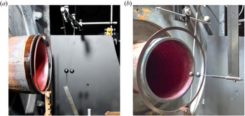
The drag and lift forces are required for the following sphere ( $S_2$). It is thus screwed until its centre of gravity on the sting of the aerodynamic balance. The balance is positioned horizontally in the flow and fixed to a triaxial displacement system as presented in figure 5.
Forces balance set-up. Pictures of a measurement of (a) the total forces, and (b) the residual forces.

The balance is positioned horizontally to avoid gravity effects, as explained by Noubel & Lago (Reference Noubel and Lago2021). Thus lift forces are measured in the  $\boldsymbol {y}$-direction, so the second sphere will be displaced in the
 $\boldsymbol {y}$-direction and not in the
 $\boldsymbol {z}$-direction as for the other experiments. Since the flow in the core is isotropic, the change in direction does not modify the physics of the shock/shock interferences or the physical values. The positioning is controlled with a camera placed on top of the test chamber.
Sphere  $S_1$ and a plate are placed in a rotary system so that the sphere is in either the flow (figure 5a) or the plate (figure 5b). The usefulness of this system will be explained in the next paragraph. The first sphere is placed as described in § 3.1 (figure 5a), but this time, to keep the same displacement area for the second sphere,
 $S_1$ off-centre from the middle of the nozzle is in the
 $\boldsymbol {y}$-direction (
 $Z=0$ mm,
 $Y=-30$ mm).
For each position of  $S_2$, two measures have to be realized: with
 $S_1$ in the flow (figure 5a), and with a plate hiding
 $S_2$ from the flow (figure 5b). The first measurement records the total drag and lift forces, including residual forces induced by the suction of the pumping group, or vibration from the pumping group. The second measurement records only the residual forces. The acquisition time, both with and without the plate, is 10 s, with acquisition frequency 1000 kHz. These two steps are repeated five times. For each module, drag and lift, values are averaged and the residual force values are subtracted from the total force to obtain the real drag and lift forces.
3.2.2. Swinging sphere method
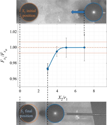
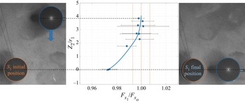
This method consists in suspending the second sphere by a wire system so that it can move freely according to the surrounding flow. The angle of deviation of the sphere will depend on the force acting on the sphere, the measurement of which allows the aerodynamic force to be deduced (Cardona & Lago Reference Cardona and Lago2022). As shown in figure 6, the swinging sphere method was employed in two different ways. In figure 6(a), the suspended sphere is the second one, in order to measure the impact of  $S_1$ over
 $S_2$. In figure 6(b), on the contrary, the first sphere is suspended, in order to measure the effect of
 $S_2$ on
 $S_1$.
Picture of the swinging sphere experiments: (a) method applied on  $S_2$ supported by a moving support; (b) method applied with
 $S_1$ supported by a fixed support, and
 $S_2$ moving.

In both cases, the suspended sphere is drilled from side to side on an axis passing through its centre. A thin, inelastic wire of 0.07 mm diameter passes through the hole in the sphere and through the hole in a hollow tube that serves as a support to hold it like a swing. This tube is positioned horizontally, parallel to the  $y$–
 $z$ plane so as to give a single degree of freedom along the
 $x$ axis. In order to avoid any movement in the
 $\boldsymbol {y}$-direction, the wire is glued to the sphere and to the stem. To obtain precise results, the sphere is positioned so that both sides of the wire have the same length, forming an isosceles triangle with the straight stem as base. This experiment is analysed from images obtained with the Kuro camera equipped with the VUV lens described in § 3.1. Despite the high stability of the flow and the equilibrium state reached by
 $S_2$, a slight movement of very small amplitude may affect the sphere. To improve the quality image definition, the images were recorded with very short acquisition times since the aim is to detect accurately moving spheres and wires. On the contrary, due to the size of each image, the duration of acquisition must not be too long so that the sets of images generated are not heavy files. A good compromise was to set the acquisition time to 20 ms per image.
For the experiment that consists in studying the movement of the sphere  $S_2$ (figure 6a),
 $S_1$ is set as for the set-up of flow visualization described in § 3.1. The tube that holds the wires of
 $S_2$ is attached to a triaxial Cartesian displacement system, which aligns
 $S_2$ with
 $S_1$ in the same vertical plane that passes through
 $Y=0$. After the flow has been established and stabilized,
 $S_2$ is first placed in its initial position, right behind
 $S_1$ in the
 $\boldsymbol {x}$-direction. The experiment then consists in moving the tube vertically, or horizontally with the displacement system with constant speed 0.8 mm s
 $^{-1}$. As
 $S_2$ is moved in the wake of
 $S_1$, the sphere progressively balances itself so that it compensates for the forces induced by the flow.
For the second experiment (figure 6b),  $S_1$ is suspended by the swinging system. The holding tube of
 $S_1$ is then fixed to the wall of the test chamber. The second sphere is held by the same moving system as the one described in § 3.1. Both spheres are placed in the same positions as described in § 2.3. In this experiment, the support of
 $S_1$ does not move, and only
 $S_1$ responds to the experienced forces. This time, it is
 $S_2$ that is displaced behind
 $S_1$ to study the impact of its positioning on the upstream sphere. For this experiment, some positions of
 $S_2$ were studied. Images were recorded with stationary positions for reasons that are explained in Appendix A.
The determination of the force value of the suspended sphere is based on the measurement of the angle of its wires with respect to the vertical, as detailed in Cardona & Lago (Reference Cardona and Lago2022). Assuming an equilibrium state of the sphere in each image (i.e. acceleration 0 m s $^{-2}$ is considered), Cardona & Lago (Reference Cardona and Lago2022) demonstrated that the drag force
 $F_x$ of the sphere is given by
 \begin{equation} F_x=m\, g \sin(\alpha). \end{equation}
With the manual detection of the wire, and automatic detection of the sphere, accuracy  $\pm$1 px for both the centre of the sphere and the wire is assumed. Consequently, the real angle is given with estimated accuracy
 $\pm 0.4^{\circ }$, and the drag force of each position with accuracy
 $\pm$0.18 mN. This method was validated by comparing the drag forces of a single sphere obtained by Cardona & Lago (Reference Cardona and Lago2022) and literature results. In the present work, the swinging method is applied to an interactive sphere (
 $S_2$) to study the effects of interaction. Results are compared to those obtained with the aerodynamic balance in the same experimental conditions in Appendix B. These two methods show a good agreement, which allows us to be confident with the results obtained with the swinging method.
3.3. Surface pressure measurement
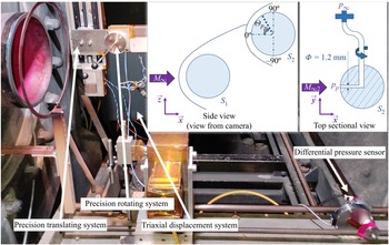
The set-up used for the measurement of wall pressure of the second sphere  $S_2$ is shown in figure 7. The purpose is to measure the pressure at the surface of the second sphere in the meridian plane for every interference type investigated. The assembly of the first sphere remains unchanged from that described in § 3.1. The second sphere is drilled as shown in the top sectional view of figure 7. A hole of 1.2 mm diameter along a radius of
 $S_2$ is made to measure wall pressure. This diameter is chosen according to two experimental constraints. The hole must be small enough to have a highly localized measurement of the pressure at the surface of
 $S_2$. At the same time, as the pressures at the surface of the sphere are very low, the diameter of the hole must be large enough to reach equilibrium with the pressure sensor, to which the pressure line is linked, in a reasonable time. A second larger hole is made perpendicular to the first, into which a stainless steel tube is inserted. This tube is used to hold the sphere in position and to connect the wall pressure measurement hole to the pressure sensor. This tube is placed on a horizontal plane and perpendicular to the flow axis. Its diameter was chosen according to two parameters: not to obstruct the flow too much, but to hold the sphere sufficiently so that it does not vibrate with the forces exerted by the flow. At the opposite end of the sphere, the tube is maintained in a precision rotating system. As can be seen on the scheme, in the side view of figure 7, this rotating system can rotate
 $S_2$ without moving it towards
 $S_1$. Therefore, the hole of
 $S_2$ moves along the perimeter of the vertical plane at its surface, allowing wall pressure measurements at different angles. The rotating system is in turn supported by a precision vertical translation system enabling the precise movement of
 $S_2$ to obtain the six types of shock/shock interference. The whole assembly is held on the triaxial displacement system. The wall pressure is measured with a pressure sensor that is placed inside the experimental chamber, out of the flow. This minimizes the distance between the measuring point and the sensor; the pressure line is connected by a flexible tube. The sensor is placed vertically on a support that absorbs vibrations, so that the membrane separating two identical pressure cavities does not undergo gravity or vibrations. The sensor is a Validyne DP103 that measures the differential pressure between the surface hole and the residual pressure in the test chamber
 $p_\infty$. The sensor measures very low pressures up to 0.0125 psi, i.e. 86 Pa, and is accurate at 0.5 % of the full scale, i.e. 0.43 Pa.
Picture and schematics of the surface pressure measurement.

For each position of  $S_2$, thus for each interference case studied, the wall pressure of
 $S_2$ was measured over an angular section ranging between
 $90^{\circ }$ and
 $-90^{\circ }$, as described in the side view in figure 7. For each angle, it is necessary to wait as long as needed to stabilize the pressure. For each position of
 $S_2$, once the pressure has been measured for all angles, the sphere is rotated to its initial angle, and a new measurement is realized to ensure that there is no deviation in values during the time of the experiment (
 $\sim$4 h).
4. Shock/shock interference analysis for a fixed longitudinal distance
4.1. Identifications of the type of shock/shock interference
In a first study (Cardona et al. Reference Cardona, Joussot and Lago2021), numerous images were recorded for a large set of positions, varying both  $X_2$ and
 $Z_2$. As investigated in the continuum regime (Edney Reference Edney1968), six different patterns were identified. Even though the results gave first knowledge of shock/shock interferences (SSIs) in a supersonic rarefied flow, the mapping of the positions of
 $S_2$ described in this previous work was not ideal. Indeed, the position grid was not fine enough. Moreover, the results were obtained for different
 $X_2$ positions, which induces a variation of the pressure perceived by
 $S_2$ along the shock of
 $S_1$. And when one moves away longitudinally from
 $S_1$, the structure of the shock of
 $S_1$ is modified because the pressure in the shock changes; it becomes more diffuse, which also affects the flow field in the wake of
 $S_1$. Therefore, the interaction of the shocks of
 $S_1$ and
 $S_2$ is also modified as a function of the position
 $X_2$. In addition to these effects, the angle of incidence of the shock from
 $S_1$ on
 $S_2$ is also changed when
 $S_2$ moves away longitudinally from
 $S_1$. All of these variations would not allow the SSI effects to be decoupled from these flow variations. However, the purpose of the present study is to evaluate the specifics of each type of interference in a rarefied flow. We therefore chose to fix the longitudinal position of
 $X_2$ of the second sphere and move it only in the vertical direction, keeping the angle of the incident shock constant. It was chosen to place the nose of
 $S_2$ 24 mm behind that of
 $S_1$ in the
 $\boldsymbol {x}$-direction, resulting in incident shock angle 25
 $^{\circ }$. As the second sphere moves down in the wake of the first one, its shock wave intersects the shock wave of
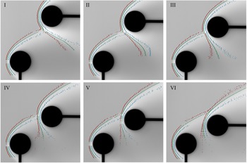
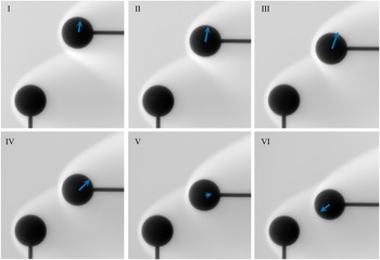
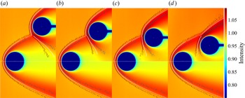
 $S_1$, in six different ways. Figure 8 shows the images obtained for the six types of interference first described by Cardona et al. (Reference Cardona, Joussot and Lago2021), and detailed more accurately in the present work.
Images of the SSIs and their detected shock waves (red indicates FS, green indicates MS, blue indicates BL).

In order to analyse SSIs qualitatively, the  $S_1$ and
 $S_2$ shock waves were superposed as shown in figure 9.
Superposition of  $S_1$ (reference case without interference) and
 $S_2$ (with interference) middle shock waves for each type of interference.

Many relative positions of  $S_2$ with respect to
 $S_1$ (
 $X_2/r_1=3$, with
 $r_1$ the radius of
 $S_1$) other than those given in figures 8 and 9 were recorded. This made it possible to classify the SSIs in terms of coordinates and thus of intersection angles
 $\varTheta _i$, as shown in figure 10. Since shock waves are thick and diffused in rarefied flows, the SSI characteristics are not as clearly defined as in the continuum regime, where pressures are higher. This means that transitions between two types of SSI are smooth and are given as a function of the angle area. Consequently, the determined angles described in figure 10 delineate transition areas.
Schematics of SSIs with the associated range of incident shock angle.

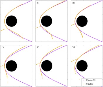
A detailed qualitative analysis of figures 9 and 8 reveals several important features.
(i) Considering the sphere
 $S_2$, its shock is not symmetrical, unlike for $S_1$. The lower flow region is affected by the presence of the first sphere, and particularly the flow conditions that it creates.
(ii) For all types of interference, from I to VI, we see that the shock angle of the lower part of the
$S_2$ shock wave increases. For types I and II, below the intersection point, the $S_2$ shock wave is pushed by the incident shock. Then, as $S_2$ descends, it enters the wake of $S_1$, where the level of rarefaction increases as the local pressure decreases. Hence the lower part of the $S_2$ shock wave is less compressed: it expands and gets thicker.(iii) For types IV, V and VI SSIs, the incident shock wave, coming from
$S_1$, interferes with the upper part of the $S_2$ shock wave ($\varTheta _i > -5^{\circ }$). For type IV, the $S_1$ and $S_2$ shock waves intersect almost perpendicularly, while for types V and VI, the two shocks go in the same direction (north-east). Either way, one part of the molecules arriving with the $S_1$ shock wave penetrates under the upper part of the $S_2$ shock wave. Consequently, the $S_2$ shock wave deviates upwards. For type VI, this effect diminishes due to the fact that as $S_2$ goes down in the wake of $S_1$, the $S_1$ shock wave will progressively go above the shock wave of $S_2$ until there is no SSI.(iv) From type I to type III, below the point of intersection (
$\varTheta < \varTheta _i$), the curvature of the $S_2$ shock wave appears to flatten, while for types V and VI, the flattening occurs above the point of intersection ($\varTheta > \varTheta _i$). This behaviour is probably related to the location of the pressure peaks deforming the shock wave of the second sphere.(v) Another peculiarity of the type I–IV patterns is the presence of a recoil zone, where the point of intersection of the shocks appears to be pushed farther ahead of
$S_2$. This seems to occur when the shock waves from $S_1$ and $S_2$ meet with different orientations, one going north-east and the other south-east. Moreover, this feature is not observable for types V and VI, where the shock waves follow the same direction (north-east).


In the following, the six interference types that have been identified will be investigated in terms of visualization, aerodynamic forces and wall pressure measurements.
4.2. Identification of points of interest and their characteristics
4.2.1. Stand-off distances
The shock-wave detection method allowed us to identify three regions of shock. On the horizontal line from the nose of the sphere (see the horizontal lines in the two schemes in figure 4), the stand-off distances ( $\varDelta$) of the foot shock (FS), middle shock (MS) and boundary layer (BL) were determined. Figure 11 presents the evolution of these stand-off distances as a function of the angle of intersection
 $\varTheta _i$, and reveals the deformation of the shock waves on the horizontal line of
 $S_2$. These results were not observed in Cardona et al. (Reference Cardona, Joussot and Lago2021) where
 $X_2$, and thus the incident shock angle, varied, suggesting that the incident shock angle tends to influence the SSI, as has been found in many other studies in the continuous regime (Edney Reference Edney1968; Keyes & Hains Reference Keyes and Hains1973; Borovoy et al. Reference Borovoy, Chinilov, Gusev, Struminskaya, Délery and Chanetz1997; Boldyrev et al. Reference Boldyrev, Borovoy, Chinilov, Gusev, Krutiy, Struminskaya, Yakovleva, Délery and Chanetz2001; Peng et al. Reference Peng, Luo, Han, Hu, Han and Jiang2020). Nevertheless, to investigate the influence of the incident shock angle under rarefied conditions, further study would be required. On the three graphs in figure 11, the black lines represent the mean value for stand-off distances of
 $S_1$, which do not change (with
 $\pm 0.154$ mm accuracy) whatever the vertical position (
 $Z_2$-coordinate) of
 $S_2$. Since
 $S_2$ has exactly the same diameter as
 $S_1$,
 $\varDelta _1$ also represents the stand-off distances that
 $S_2$ should have without any interactions.
Shock stand-off distances of  $S_2$ according to the type of interference: (a) foot shock, (b) middle shock, and (c) boundary layer.

As observed, the stand-off distances for the sphere  $S_2$ (
 $\varDelta _2$) are strongly impacted. Note that
 $\varDelta _{BL_2}$ is almost constant (figure 11c), except for type VI SSIs, where an increase can be observed. It corresponds to positions where
 $S_2$ enters the wake of
 $S_1$ more deeply, i.e. where the local mean free path also increases. This is in agreement with Rembaut, Joussot & Lago (Reference Rembaut, Joussot and Lago2020) and Akhlaghi & Roohi (Reference Akhlaghi and Roohi2021) who showed that an increase in the rarefaction level leads to an increase in
 $\varDelta$, and therefore to an increase in
 $\varDelta _2$ for type VI SSIs.
For all the five other types of interference, the analysis is based on  $\varDelta _{FS_2}$ and
 $\varDelta _{MS_2}$. For type I SSIs, the stagnation line of
 $S_2$ is not impacted. The area of interaction affects only a small area of the lower part of the shock. Then, from type II to type III,
 $\varDelta _2$ increases strongly. From a detailed analysis of the schematics of SSI in figure 10, it seems that the shock wave of
 $S_1$ penetrates in between the surface of
 $S_2$ and its shock wave by going up, pushing it away at the nose. The range of angles of type IV SSIs seems to be a transitional area, where the stand-off distances suddenly decrease. This could be due to the particular impact where the two shock waves meet almost perpendicularly around the nose of
 $S_2$. This creates a V-shaped deformation of the shock, which seems pushed away from
 $S_2$ surface above its nose. But at the nose, the strong incident shock wave penetrates deeper into the shock wave of
 $S_2$, decreasing the stand-off distances of both its FS and MS. Types V and VI SSIs do not impact the shock wave shape much at the stagnation point. As discussed above, the increase in
 $\varDelta$ is due mostly to the increase in rarefaction level.
4.2.2. Distances between the interaction area and the surface of $S_2$

Figure 12 shows the points of interest  $P_i$ and
 $P_{ml}$ that we identified in figure 4. Distances
 $d_i$ and
 $d_{ml}$ were determined on the
 $S_2$ shock wave for each angle of intersection
 $\varTheta _i$. Here,
 $P_i$ is located at the intersection between the middle of the shock waves so it refers to the middle shock region, and
 $P_{ml}$ is the most luminous point in the intersection area so it refers to the boundary layer region. Thus
 $d_i$ and
 $d_{ml}$ are, respectively, compared to
 $d_{MS_1}$ and to
 $d_{BL_1}$, the distances of the shock wave without SSI.
Distances of (a) the interaction point and (b) the most luminous point in the shock/shock interaction area from the surface of the sphere, according to the type of interference.

First, it is important to note that  $d_i$ remains greater than or equal to its reference value (
 $d_{{MS}_1}$), while this is not the case for
 $d_{ml}$ as it is smaller than its reference value (
 $d_{{BL}_1}$) from types III to VI SSI. This means that in the intersection area, the middle of the shock is mostly pushed away from the surface of
 $S_2$, while the boundary layer is mostly pushed towards it. Consequently, in this area, shock waves are thicker and more diffuse, increasing the viscous effect at the wall of the sphere.
Also, another remarkable feature of the curves in figure 12 is the V-shape that appears around the interference angle  $0^{\circ }$. This area shows a very localized increase in the stand-off distance for both the shock interaction and the point of greatest brightness that reflects the point of greatest density. This feature can also be observed in the specific shape of the type IV SSI shown in figure 10 in a schematic way, and in the image in figure 8. Curiously, it is more marked than any other aspects of SSI shapes. This is consistent with the fact that the type IV SSI is a transition region where the interaction of shocks exhibits compression, as can be seen in figure 11, where the distances of the different shock regions become smaller than the reference distances.
4.2.3. Intensity levels in the intersection area
Another interesting observation that deserves analysis is the distribution of the light intensity in the area of the shock interaction. Even if the intensity is not exactly proportional to the density, it gives information concerning the impact of SSI on the local density. In figure 13, the intensity level of  $P_{ml}$ (
 $I_{ml}$ in figure 13a) and of the most luminous point passing by the nose of
 $S_2$ (
 $I_{0_2}$ in figure 13b) are plotted. In order to compare the intensity levels of the different images, their values have been normalized with
 $I_{0_1}$ of each image. It should be noted that
 $I_{0_1}$, located at the stagnation line of
 $S_1$, is the densest point of a single sphere, and its value is the one that
 $S_2$ should have without any interaction.
Intensity values of the most luminous points (a) in the shock/shock interaction area, and (b) on the stagnation line, according to the type of interference.

As shown in figure 13, the two tendencies are the same: the slopes increase from type I to IV, and then decrease from type IV to VI. Figure 13(b) shows the light intensity at the  $S_2$ stagnation point normalized to that of
 $S_1$. The curve shows a maximum for the type IV SSI, which is representative, for this type of interaction, of an increase in local density in front of
 $S_2$. Figure 13(a) presents the evolution of
 $I_{ml}$, showing that whatever the type of SSI, the local density in the intersection zone of the shocks is higher than the maximum density observed at the stagnation point of the
 $S_1$ sphere taken as reference. On the other hand, the graph in figure 13(b) shows for type I, where the sphere is almost out of the influence of the shock wave
 $S_1$, that the densities of the two stagnation points are equal. This is consistent, since the free flows seen by
 $S_1$ and
 $S_2$ are the same. Then, from type II to type VI, the intensity values vary in the same way as for
 $P_{ml}$. Approaching type VI, the density at
 $P_{0_2}$ becomes lower than that at
 $P_{0_1}$, leading to an increase in separation distances due to a higher level of rarefaction. Also, the mean free path increases, and the free flux density decreases as well as the local density in the shock wave of
 $S_2$.
4.3. Drag and lift
4.3.1. Drag and lift analysis
The aerodynamic balance described in § 3.2 was used to measure the drag and lift forces of  $S_1$ alone, and of
 $S_2$ interacting with
 $S_1$. From the previous images, the six relative positions of the sphere were selected to observe the impact of the different SSI on the aerodynamic forces. Drag (
 $F_{x_2}$) and lift (
 $F_{z_2}$) force values of sphere
 $S_2$ are presented in figures 14(a,b), respectively. Black lines with the values
 $F_{x_0}$ and
 $F_{z_0}$ are the drag and lift forces undergone by a single sphere without any interactions. They represent the forces that the sphere
 $S_2$ would have experienced without any interaction.
(a) Drag and (b) lift forces of  $S_2$ measured with thrust device.

The evolution of the drag force shows that for type I,  $F_{x_2}$ is almost the same as the reference value. This result was expected since both spheres see almost the same free flow (with the difference of a slight impact of the
 $S_1$ shock wave on
 $S_2$). From SSI types I to IV, as
 $S_2$ goes down and interacts with the
 $S_1$ shock wave,
 $F_{x_2}$ increases. It reaches a maximum for a type IV SSI, the transition area highlighted particularly in § 4.2. For types V and VI, the drag force suddenly decreases, reaching values lower than
 $F_{x_0}$. Again, this is due to the fact that
 $S_2$ goes deeper into the wake of
 $S_1$, where the flow is more rarefied, and presumably reaches speeds that are lower than the free-stream flow. As a result, the forces experienced by
 $S_2$ behind
 $S_1$ (in the
 $\boldsymbol {x}$-direction) decrease greatly, suggesting that when a fragmented piece of debris remains behind a parent piece of debris, the latter protects it from being damaged by the free flow. In figure 15, the luminous profile along the vertical axis
 $X_2/r_1=3$, and the drag force profile, are plotted, both according to
 $Z_2$. Since the luminous intensity is the reflection of the local density, no recompression area is observed in the wake of
 $S_1$. Therefore, since the profile of the drag forces follows the profile of the intensity, the decrease of the altitude of the sphere
 $S_2$ leads to the decrease of the force
 $F_{x_2}$. This statement will be confirmed later in this work with the oscillating sphere results.
Drag force and luminous intensity profiles along the vertical axis  $X_2/r_1=3$.

With respect to lift forces, for types I–III,  $S_2$ is mainly above the shock wave of
 $S_1$, and after, it is mainly below. Therefore, one would expect
 $S_2$ to be respectively repelled or attracted in the
 $\boldsymbol {z}$-direction by ricocheting off the shock wave of
 $S_1$, as can be observed in the continuous regime (Register et al. Reference Register, Aftosmis, Stern, Brock, Seltner, Willems, Guelhan and Mathias2020). But in fact, since the shock wave from
 $S_1$ is thick and diffuse, it does not represent a clear boundary that would block
 $S_2$ in the wake of
 $S_1$. For this reason, the sign of the lift force of
 $S_2$ does not change as it approaches the shock of
 $S_1$ from above or below, but simply decreases. Nevertheless, it could undergo a change of sign for a type VI SSI, but this would be due not to shock/impact interference but to the protection created by
 $S_1$, when
 $S_2$ is in its wake and close to the axis of
 $S_1$.
According to the forces undergone by  $S_2$ and
 $S_1$, one can deduce the displacement of
 $S_2$ toward
 $S_1$ as follows:
(i) if
$F_{x_2}< F_{x_0}$, then $S_2$ approaches $S_1$ in the $\boldsymbol {x}$-direction ($\Leftarrow$)(ii) if
$F_{x_2}>F_{x_0}$, then $S_2$ moves away from $S_1$ in the $\boldsymbol {x}$-direction ($\Rightarrow$)(iii) if
$F_{z_2}< F_{z_0}$, then $S_2$ approaches $S_1$ in the $\boldsymbol {z}$-direction ($\Downarrow$)(iv) if
$F_{z_2}>F_{z_0}$, then $S_2$ moves away from $S_1$ in the $\boldsymbol {z}$-direction ($\Uparrow$).


Taking into account both the values and directions of each force, the resulting forces were calculated in the  $S_1$ referential, and the results are drawn in figure 16, giving information on the direction of
 $S_2$ towards
 $S_1$. As can be seen, when
 $S_2$ and its shock are enveloped in the shock of
 $S_1$, it is attracted to the first sphere.
Calculated displacement of  $S_2$ in
 $S_1$ reference frame according to the shock/shock interaction type.

4.3.2. Comparison with the continuum regime
Fisher (Reference Fisher2019) studied the SSIs of Edney in a continuum regime at Mach 5. His experiment consists in releasing a sphere that flies freely in the flow field generated by a primary sphere. This work allows us to compare SSI depending on the level of rarefaction, since drag forces were measured.
In the work of Fisher (Reference Fisher2019), the drag coefficient was calculated with  $C_d=\tfrac {1}{2}{F_x}/$
 $({\rho _{\infty } V_{\infty }^2 S})$, where
 $\rho _{\infty }$ and
 $V_{\infty }$ are the values in the free-stream flow (upstream of
 $S_1$), and
 $S={\rm \pi} ({D}/{2})^2$. Note that this method does not take into account the local flow seen by
 $S_2$ moving in the flow generated by
 $S_1$. Since free-stream flow conditions impact directly the flow generated downstream of
 $S_1$, it is questionable if this parameter is effectively representative of the aerodynamics of
 $S_2$. Nevertheless, it allows us to compare results with the literature, where this method is mostly used. In our conditions, the drag coefficient of a single sphere is 1.35, while Fisher's is about 0.88. For both results, the drag coefficient of
 $S_2$ (
 $C_{d_2}$) is normalized by that of a single sphere (
 $C_{d_o}$). In figure 17, it is clear that the trends of all the curves are similar: for type I, the drag force of
 $S_2$ is almost that of the sphere alone in the free stream; in the wake of the sphere
 $S_1$, the dynamic pressure decreases as one moves towards the centre of the flow, i.e. towards a type VI interaction. The flow therefore becomes rarefied; the viscosity increases as well as the mean free path. As the local density and velocity decrease, the forces become smaller. The second sphere will experience weaker forces and, in a way,
 $S_2$ will be ‘protected’ by remaining in the wake of the first sphere,
 $S_1$. So the impact of the SSI, in terms of drag coefficients, is similar for both regimes. Nevertheless, this analysis has to be taken with caution for two reasons. On the one hand, the trajectory described by the sphere of Fisher is different from ours. On the other hand, the drag coefficients are given according to a type of SSI, but not in terms of location. As the shock wave of
 $S_1$ is thicker and more diffuse in a rarefied flow, the area where SSI occurs will be larger than in a continuum regime, expanding the area of high drag forces. This hypothesis seems to be confirmed by the results of Laurence & Deiterding (Reference Laurence and Deiterding2011).
Drag coefficient of the present work on the vertical axis  $X_2/r_1=3$, compared with the results of Fisher (Reference Fisher2019), with variable coordinates.

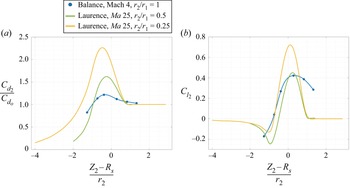
In figures 18(a,b), respectively, the drag and lift coefficients are plotted according to the normalized distance of  $S_2$ towards the incident bow shock. Here,
 $Z_2$ is the altitude of
 $S_2$ towards
 $S_1$,
 $R_s$ is the altitude of the shock wave (middle shock in our case), and
 $r_2$ is the radius of
 $S_2$. Both results concern the vertical axis
 $X_2/D_1=1.5$ (
 $X_2/r_1=3$). As far as drag is concerned, it can be seen that the maxima are obtained globally at the same location for all cases, but their amplitude varies inversely with the radius ratios of the spheres. The two iso-Mach curves have roughly the same shape, although they were obtained for different sphere radius ratios. This suggests that for ratio 1 , the corresponding curve would also have the same shape but would show a smaller maximum value. The curve obtained in the present work has a slightly different shape from the other two, with a wider curvature around the maximum, which could be due to rarefaction effects. However, this remains a hypothesis because it was performed at a lower Mach number. Regarding the lift coefficients, at iso-Mach, the maxima and minima have the same locations, and again with very similar shapes, as for the drag. Nevertheless, the maximum lift is observed for the same location, the curve does not have a minimum, and especially the shape of the curve around the maximum is less sharp and wider. This last point, observed for both the drag and the lift, might be due to the important decrease in Mach number, but in any case, if they exist, these effects are coupled with the increase in the rarefaction level that thickens the incident shock wave, and thus enlarge the area where the aerodynamic coefficients of
 $S_2$ are impacted.
Drag and lift coefficients of the present work for a longitudinal distance of 1.5 diameters, compared with the results of Laurence & Deiterding (Reference Laurence and Deiterding2011).

4.4. Surface pressure
4.4.1. Wall pressure analysis
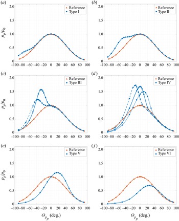
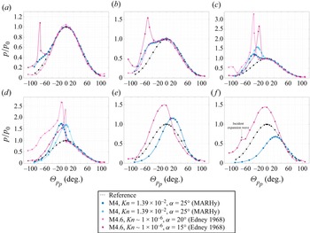
The pressure distribution at the surface of  $S_2$ was measured for the same six locations as those already investigated. However, three other relative positions were explored to better describe the transitions between the different types of SSI, in particular between types III and IV, and between types IV and V. The pressures were also measured for a single sphere, representative of the reference wall pressure distribution. Figure 19 describes, for each type of SSI, the pressure distribution at the surface of
 $S_2$ in blue, along with the reference case in orange. The wall pressure values (
 $p_p$) are normalized with the stagnation pressure (
 $p_0$) which is 56.17 Pa. The wall pressure distributions are given as functions of the angle of the measurement point (
 $\varTheta _{p_p}$) with respect to the surface of
 $S_2$,
 $0^{\circ }$ being taken with respect to the nose of the sphere.
Pressure distributions for the six types of SSIs and for a single sphere (reference case).

The pressure distribution reveals two different behaviours. Concerning types I, II and III, the surface pressure is disturbed only on the lower part of the sphere ( $\varTheta _{p_p}<0^{\circ }$). For these three types, the wall pressure is higher than the reference case in the interference area. After this increase, the wall pressure returns to the reference behaviour. Pressure distribution clearly presents two peaks: one which corresponds to the intersection zone of two shocks, and the other which corresponds to the nose of the sphere (at the stagnation point). In the first case, the peak is not, mathematically speaking, a maximum, but it is obtained with the minimum of the pressure derivative according to the angle, corresponding to the interaction area. For types IV, V and VI SSI, the pressure distributions are modified globally, resulting in only one maximum corresponding to the intersection area. Outside the interference area, in the lower part of
 $S_2$ (
 $\varTheta _{p_p}<0^{\circ }$), values are lower than those of the reference case. At maximum, a great peak is reached, and then the slope tends to stick to the reference value. For types IV and V, the peak is clearly higher than the reference maximum value, while type VI is lower, which is coherent with the fact that
 $S_2$ penetrates deeper into the wake of
 $S_1$, i.e. when the flow is more rarefied.
Pressure peaks in the interference area ( $p_{p_{max, interf}}$) are plotted according to
 $\varTheta _{i}$ in figure 20(a). The angle of these peaks (
 $\varTheta _{p_{p_{max, interf}}}$) are also plotted according to
 $\varTheta _{i}$ in figure 20(b). Due to the thickness of the shock wave, the angles given as frontier (figure 10) are not clear delimitations; this is why the three positions of type IV presented in figure 19 are not located in the exact
 $\varTheta _{i}$ range. Nevertheless, regarding the shape of the pressure distribution of the three points discussed for type IV, they seem to follow the same behaviour. With this assumption, we will henceforth consider them as representative of a type IV SSI. Figure 20(a) shows an increase from I to IV and then a decrease of the maximum pressure in the intersection area. The maximum pressure peak is reached when middle shock waves interact at approximately
 $-5^{\circ }$ from the horizontal, which corresponds to a type IV SSI. Figure 20(b) plots the location of the pressure peak at the surface of
 $S_2$ as a function of the angle of the interaction point. As can be observed, the curve presents two distinct regions with two different slopes. The first area corresponds to types I to IV, where the value of
 $\varTheta _{p_{p_{max, interf}}}$ increases until it reaches the same value as the angle of intersection. From this point, the curve has a gentler slope for types V and VI, since
 $\varTheta _{p_{p_{max, interf}}}$ increases by
 $20^{\circ }$ for an increase of
 $\varTheta _i$ by
 $60^{\circ }$. One can notice that the maximum pressure is located mostly on the lower part of the sphere and does not seem to go higher than
 $25^{\circ }$ from the stagnation point, even if the intersection angle is on the higher part of the sphere.
(a) Maximum surface pressure  $p_{p_{max, interf}}$ and (b) its angle
 $\varTheta _{p_{p_{max, interf}}}$ according to the interaction angle
 $\varTheta _{i}$.

4.4.2. Comparison with the continuum regime
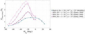
A comparison of the pressure distribution of the present work has been made with the results of Edney (Reference Edney1968) (see Appendix A). His work, based on the interaction of an oblique incident shock with the bow shock of a hemisphere, indicates a similar behaviour for SSI types I to III, with more pronounced pressures values, and thinner pressure peaks. The real difference is observed for SSI types IV to VI. In particular, the specific pressure distribution of the continuum regime seems to vanish completely in our rarefied conditions, appearing a lot like a type V or VI. This might be due to the thicker boundary layer that would prevent a supersonic jet from impinging at the wall of  $S_2$. Thus the type IV interference might be disappearing as the level of rarefaction increases, as suggested by Gusev & Erofeev (Reference Gusev and Erofeev2004) or White & Kontis (Reference White and Kontis2018), who studied the impact of an incident shock on a cylinder at Knudsen numbers equivalent to our conditions.
Figure 21 focuses more specifically on pressure peaks. It is obvious, whatever the angle of incident shock, that the continuum case presents higher values of pressure peaks. Their repartition at the wall of  $S_2$ is more localized: it concerns a region of about
 $10^{\circ }$, against
 $40^{\circ }$ in our case. Also, the maximal pressure peak is located on a lower angle (about
 $-25^{\circ }$) than the one that we observed in the rarefied regime (about
 $-10^{\circ }$). These differences are consistent with the increase in the thickness of the shock wave due to an increase in the level of rarefaction: the impact of the SSI is localized not in one point, but in a zone leading to a decrease in the impact of the boundary layer of the second sphere at its surface, and therefore also the decrease in wall pressure.
Pressure peak distribution, comparison with results of Edney (Reference Edney1968) in a continuum regime.

4.5. Discussion regarding the results obtained for $X_2/r_1=3$

Analysis of the results presented in figures 11–14, 19 and 20 allows us to make several observations and analyse the different SSIs as follows.
(i) Type I does not impact
$S_2$ much. The sphere is mostly located in the free stream and thus suffers more from it than from the interaction with the $S_1$ shock wave. Looking at the wall pressure distribution, it can be seen that the values are slightly higher in the interference area, located on the lower part of the sphere, which explains the lift force that is a bit higher than the reference.(ii) Type II implies a recoil of the
$S_2$ shock wave from its surface, at the nose of the sphere but also in the interaction area; only the BL seems to decrease. The local density in both areas also seems to increase, along with the drag force. The lift force also increases, but this is due to a greater modification ($p_{p_{max, interf}}\simeq p_0$) of the wall pressure on the lower part of $S_2$.(iii) Type III shows the same tendency as type II. The stand-off distances reach a maximum (except for BL) for
$\varTheta _{i}\simeq -10^{\circ }$, which corresponds to the angle of minimum distance of the BL in the interaction area. The drag force keeps increasing as $S_2$ goes down, while the lift force reaches a maximum $\varTheta _{i}\simeq -20^{\circ }$, and then decreases. Looking at the pressure distribution, it is noticeable that the great pressure peak ($p_{p_{max, interf}}>p_0$) displaces towards the centre of the sphere, decreasing the lift effect that had the incident shock for higher positions.(iv) Type IV shows strong variation in shock distances. Stand-off distances decrease drastically to reach a minimum for
$\varTheta _{i}\simeq 20^{\circ }$. A recoil of the interaction point and of the BL in the interaction area is observed, with local maximum for $\varTheta _{i}\simeq 0^{\circ }$. Then both decrease until their reference value. The BL seems less impacted than the MS. The maximum at $\varTheta _{i}\simeq 0^{\circ }$ also corresponds to a maximal density in the interaction area and at the nose of $S_2$. It also corresponds to a maximal drag force and a maximal pressure peak. The strong compression of the shock wave might be the reflection of the drag force and pressure maximum. After this specific location corresponding to $\varTheta _{i}\simeq 0^{\circ }$, the density, the forces and the pressure all decrease.(v) Types V and VI are similar SSIs. They both present an increase in the stand-off distances, along with a decrease in the local densities corresponding to an increase of the rarefaction level since they entered the wake of
$S_1$. The drag and lift forces decrease, even reaching values that are lower than the reference. The global modification of the wall conditions decreases the maximal pressure peak. For $\varTheta _{i}>40^{\circ }$, the stagnation pressure is no longer reached, as for the reference drag force.


5. Drag force analysis with the swinging sphere experiment
In a previous study, Cardona & Lago (Reference Cardona and Lago2022) explored the swinging sphere method (described in § 3.2.1) applied to a sphere moving in the wake of another one. The force measurements obtained previously with this method were compared to those obtained with another device: the aerodynamic balance (described in § 3.2.2). The validation of the swinging method shown in Appendix B will make it possible to explore other changes in the aerodynamics of debris when an interaction with other debris exists. This method can be applied on both the first and second spheres since this force measurement is non-intrusive.
5.1. Impact of $S_1$ on $S_2$ aerodynamics


To measure the impact of  $S_1$ on
 $S_2$ aerodynamics, the swinging method was applied on a certain number of trajectories. The support of
 $S_2$, initially placed in a chosen position, is then moved in the
 $\boldsymbol {x}$- or
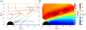
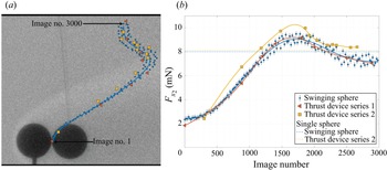
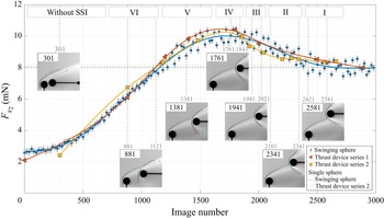
 $\boldsymbol {z}$-direction. In figure 22(a), the mean trajectories described by
 $S_2$ are plotted along with its mean drag force values. Values are given with maximum inaccuracy
 $\pm 0.6$ mN, estimated with the dispersion of the measured points (see figure 33). Note that in the calculation of the drag forces with the swinging technique, we did not consider the lift forces. Since the maximal lift force is 2.5 mN, it represents 8.9 % of the sphere weight, which corresponds to maximal error 0.84 mN on the drag forces. The mapping in figure 22(b) is obtained by interpolating these results. As can be observed, the mapping is not well defined, which is due to an insufficient number of measures. Nevertheless, it allows us to have first knowledge of the drag forces endured by a sphere in interaction with another. On the mapping are plotted the three regions of the
 $S_1$ shock wave. As can be seen, the maximum drag force is reached in the shock wave regions. When above the shock wave, the
 $S_2$ drag force is that of the reference case; when under, the
 $S_2$ drag force decreases until minimum value 2.4 mN. Except around the incident shock, there is no increase in
 $F_x$. This confirms that, due to the rarefaction level, there is no recompression wave in the wake of
 $S_1$. This marks a great difference with the continuum regime.
(a) Plot of  $S_2$ mean drag forces according to location on the different swinging trajectories. (b) Interpolated mapping of the drag force and drag coefficient.

With the use of the swinging method, we can also observe some behaviours in the wake of the  $S_1$ flow. Looking at the swinging trajectory where
 $S_2$ is displaced horizontally in the
 $\boldsymbol {x}$-direction (
 $Z_2/r_1=0$), no change of drag forces is observed. If there were some recirculation, then we should have observed, at one point, a change in the sign of the angle of
 $S_2$ wires,
 $S_2$ being pushed towards
 $S_1$ by the recirculation. As this is not the case, we might think that there is no recirculation behind
 $S_1$. This hypothesis would be consistent with previous studies from the literature, where numerical and experimental studies were carried out to understand the evolution of the wake structure of a sphere, under hypersonic and rarefied flow conditions with Reynolds numbers ranging between
 $194$ and
 $2129$. Experimentally, the wake of a sphere was analysed with Pitot pressure measurements and hot wire velocities (Muthoo & Brundin Reference Muthoo and Brundin1974). The numerical works were carried out with the direct simulation Monte Carlo method, some test cases of which were validated by the experimental results (Reeves & Lees Reference Reeves and Lees1965; Dogra et al. Reference Dogra, Moss, Wilmoth and Price1994). All the results showed that the wake shows neither separation nor recirculation in the range of Reynolds numbers studied by the different authors. The same conclusions can be applied to our experimental conditions where the Reynolds number is
 $294.5$.
As explained in Appendix B, to validate the swinging method, some measurements were realized with the aerodynamic balance on a chosen trajectory: initial position ( $X_2/r_1=2$,
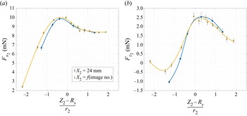
 $Z_2/r_1=0$) and support moved up. Thanks to these measurements, we obtained the drag, but also the lift forces on this trajectory. Figure 23 presents their values (yellow squares) according to the normalized vertical distance of
 $S_2$ towards the middle shock. The value obtained for
 $X_2/r_1=3$ have been superposed to evaluate the evolution of the drag and lift forces according to the longitudinal distance. As can be observed, the variation of the longitudinal distance (
 $X_2=f(\text {image no.})$) does not affect much the distribution of forces towards the middle shock of
 $S_1$. For both the drag and the lift, only a slight increase in the values is observable when
 $S_2$ is located under the
 $S_1$ shock wave.
(a) Drag and (b) lift forces of  $S_2$ on the swinging sphere trajectory (
 $X_2=f(\text {image no.})$) and on the vertical axis
 $X_2=24$ mm (
 $X_2/r_1=3$).

Figure 24 shows the locations of  $S_2$ where we measured the results of figure 23. It can be seen that the only point corresponding to
 $X_2/r_1<3$ is the lowest one (
 $({Z_2-R_s})/{r_2} = -2.2$). This means that the increase in drag is due to an increase in the diffusion of the
 $S_1$ shock wave as we look downstream, impacting
 $S_2$ aerodynamics on a wider area. Nevertheless, the diffusion of the
 $S_1$ shock wave downstream also implies a decrease in the local pressure in the shock wave. This is why we observe lower negative lift on the low position of
 $S_2$, and lower positive lift on the higher position of
 $S_2$. Nevertheless, the little impact of the longitudinal distance of
 $S_2$ shows that the flow field generated by
 $S_1$ can affect a following object in a wide area.
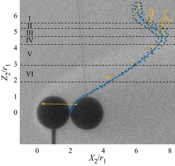
Calculated displacement (yellow arrows) of  $S_2$ in the
 $S_1$ reference frame according to its position on the swinging trajectory (blue line).

Thanks to the drag and lift measurements, in figure 24 are also plotted the local displacement of  $S_2$ towards
 $S_1$. From
 $Z_2/r_1=0$ to the transition between types VI and V, the second sphere seems attracted by
 $S_1$. As shown in § 4.4, for this type VI SSI and lower position, the maximal wall pressure is lower than the reference case due to a higher local rarefaction level. As there is no observed recompression area,
 $S_2$ is less repulsed than
 $S_1$ in the
 $\boldsymbol {x}$-direction, and so they will remain close to each other. Also, as the repartition of pressure is located mostly on the upper part of
 $S_2$, it is pushed downwards. So
 $S_2$ also gets close to
 $S_1$ in the
 $\boldsymbol {z}$-direction.
Between types VI and V, the results seem to show that there is a transition zone where the direction of  $S_2$ reverses. Referring to the different data for the position of
 $X_2/r_1=3$ and
 $\varTheta _{i} \simeq 40^{\circ }$, we observed in § 4.5 that the local density (figure 13b), the drag and lift forces (figure 14), and the pressure peak (figure 20) all reach values equal to those in the reference case. At this particular position,
 $S_2$ does not move relative to
 $S_1$, so the two spheres follow the same flight path. It is possible that these specific flight conditions lead to an equilibrium position, where
 $S_1$ and
 $S_2$ fly together without moving away from each other. As the wall pressure distribution around the sphere
 $S_2$ is not axisymmetric, one could think that a skin friction effect located on the lower part of the sphere could compensate the wall pressure forces located on the upper part of the sphere, leading to a local equilibrium. This effect seems to be confirmed by the behaviour of type V SSI measurements. By analysing further the pressure data of this interaction, we calculated that 66 % of the wall pressure contribution corresponds to the half-sphere on the upper part of
 $S_2$, which is still not consistent with a positive lift. In the continuum regime, the lift forces are driven mostly by the pressure contribution. However, in the present case, results seem to suggest a strong implication of the viscous effects, still not well understood, marking a difference with the continuum regime. It is probable that the viscous effects might act mostly on the lower part of
 $S_2$, balancing the wall pressure that acts on its upper part, leading to a positive lift. Then, from type IV to I and beyond,
 $S_2$ is pushed away from
 $S_1$ in the
 $\boldsymbol {x}$- and
 $\boldsymbol {z}$-directions. In the
 $\boldsymbol {x}$-direction, this is understandable since wall pressures are higher than the reference case. In the
 $\boldsymbol {z}$-direction, since pressure peaks are located on the lower part of
 $S_2$ for type III to I, we also easily understand the positive lift forces.
5.2. Impact of $S_2$ on $S_1$ aerodynamics


Whether in hydrodynamics (Zhu, Liang & Fan Reference Zhu, Liang and Fan1994) or aerodynamics (Golubev Reference Golubev2012), studies demonstrated that the location of  $S_2$ around
 $S_1$ impacts directly the drag forces endured by
 $S_1$. The swinging method being a non-intrusive way to measure drag forces, it can be applied to
 $S_1$ with the presence of
 $S_2$ in its flow. In this way, we can observe the behaviour of
 $S_1$ while moving
 $S_2$ longitudinally on the axis
 $Z_2/r_1=0$, and vertically on the axis
 $X_2/r_1=3$, to complete our study.
5.2.1. Case $Z_2/r_1=0$

The sphere  $S_2$ was first displaced on the horizontal axis (
 $Z_2/r_1=0$), which corresponds to the study by Golubev (Reference Golubev2012). Four locations of
 $S_2$ were studied, and the results are given in figure 25. Here, we present the drag force measured for the swinging sphere
 $S_1$ according to the relative position of
 $S_2$. Figure 26 shows the normalized enhanced images corresponding to these positions. They allow us to better understand the physics of the flow field, since they are compared to images of a single sphere in the flow.
Drag forces of  $S_1$ according to
 $X_2$, the position of
 $S_2$ relative to
 $S_1$ in the
 $\boldsymbol {x}$-direction (
 $Z_2/r_1=0$).

Normalized images with jet colour map and detection of shock waves. Top images of (a–d) show  $X_2/r_1=7, 5, 4, 3$ mm, respectively, and
 $Z_2/r_1=0$. Bottom images show single sphere.

As observed in figure 25, when  $S_2$ is far behind
 $S_1$, the latter is confronted by the same drag force as when it is alone in the flow. As
 $S_2$ gets closer, it reaches a point (around
 $X_2/r_1=4.6$) where it begins to affect the aerodynamics of
 $S_1$. Gradually, the
 $S_1$ drag force decreases. By observing the images of figure 26, a few things are noticeable. When
 $S_2$ is far enough from
 $S_1$ (figures 26a,b) not to disturb the
 $S_1$ drag force, it seems that the wake
 $S_1$ is not modified in at least the first diameter behind it. The
 $S_2$ compression wave is visible and shows the sign of a highly rarefied flow, with a great thickening of the wave and a great stand-off distance: 6.7 mm for figure 26(a), and 5.8 mm for figure 26(b). As
 $S_2$ gets closer to
 $S_1$ and enters a more rarefied flow with a lower velocity, the shock wave of
 $S_2$ has difficulty developing, but a compression is still visible upstream of
 $S_2$. The few molecules that constitute this compression might create a viscous layer that pushes
 $S_1$ upstream. Another point that might induce the variation of drag force is the merging of the incident shock with the compression wave induced by
 $S_2$.
Golubev (Reference Golubev2012) calculated the  $S_1$ drag force in a continuum regime. His results, shown and compared to ours in figure 27, were obtained for different Mach numbers but the same Reynolds number. In the continuum regime, the inter-sphere distance for which the drag coefficient of
 $S_1$ has a value equal to the reference is the same, whatever the Mach number. These three curves also show that the influence of the presence of
 $S_2$ is all the more important as the Mach number decreases. The curve obtained in this work, at Mach 4 in the rarefied regime, shows that the distance for which the drag coefficient of
 $S_1$ has a value equal to that of the reference drag is greater than that obtained at the same Mach number in the continuum regime. Comparison of the iso-Mach curves also shows that the slopes show that the influence of
 $S_2$ is substantially the same; meanwhile, the value of the normalized drag coefficient of
 $S_1$ is greater in the continuum regime.
Dimensionless drag force of  $S_1$ according the dimensionless distance between spheres
 $l$.

5.2.2. Case $X_2/r_1=3$

In the same manner as for the previous case,  $S_2$ is moved behind
 $S_1$, this time vertically on the axis
 $X_2/r_1=3$. Results of the measured
 $S_1$ drag force are plotted in figure 28 according the position of
 $S_2$. First,
 $S_2$ is placed so that it does not act on
 $S_1$, which does not displace itself. As
 $S_2$ is moved down, and gets closer to
 $S_1$, the swinging sphere moves ahead, as it does when
 $S_2$ is close behind it on the axis
 $Z_2/r_1=0$. With the normalized enhanced images of figure 29, an analysis equivalent to that from the case
 $Z_2/r_1=0$ can be made. As
 $S_2$ gets down, the lower part of the
 $S_2$ shock wave modifies the wake of
 $S_1$ by intensifying the density in its wake.
Drag forces of  $S_1$ according to the position of
 $S_2$ in the
 $\boldsymbol {z}$-direction (
 $X_2/r_1=3$).

Normalized images with jet colour map and detection of shock waves. Top images in (a–d) show  $Z_2/r_1=3.77, 3.25, 2.59, 1.74$ mm, respectively, and
 $X_2/r_1=3$. Bottom images show single sphere.

The cases where  $S_2$ locations generate SSIs do not seem to affect the drag of
 $S_1$. Indeed, we observe 3 % of drag variation whether for displacement in the axis
 $Z_2/r_1=0$, where there is no SSI, or in the axis
 $X_2/r_1=3$, where there is. This variation is not really significant, but is still interesting. In the case of space debris re-entry, it would mean that the aerodynamics of a parent piece of debris, and thus its trajectory, depends on the location of the fragments debris. These fragments can be a single object, but more often they are clouds of fragments for which the modification of
 $S_1$ aerodynamics might not be negligible.
6. Conclusion
This work presents an experimental investigation of SSIs between two spheres in a supersonic slip regime. The purpose was to analyse the influence of viscous effects on the interference properties first described by Edney (Reference Edney1968), and still much studied today, particularly in the continuum regime.
These experiments were carried out in the MARHy wind tunnel, and many results were obtained in a supersonic rarefied flow. Free-stream conditions result in a Mach 4 steady flow with static pressure 2.67 Pa, corresponding to the rarefaction degree of fragmentation altitudes. Considering debris that fragments at 76 km altitude, the models used represent two spheres of about 1 m diameter interacting with each other. This study allowed a better understanding of the different types of SSIs, and of their effects on the aerodynamics of space debris re-entry.
This study is divided into two main parts:
(i) the analysis of SSIs for a fixed longitudinal distance that induces a constant incident shock angle of
$25^{\circ }$(ii) the analysis of the drag forces with the swinging sphere experiment.

Despite the rarefaction effects, the patterns of SSI described by Edney (Reference Edney1968) are still observed in our conditions. Nevertheless, our experimental visualization technique does not allow us to observe any supersonic jet or recompression wave in between the shock and the surface of the interacting object. The distribution of wall pressure tends to confirm that there is no jet impinging at the surface of the sphere, since the particular distribution of the type IV SSI seen in the continuum regime vanishes in our conditions.
Concerning the wall pressure, some differences should be pointed out: the distribution is smoother, with lower pressure peaks. It is to be noted that for type V and VI SSIs, the pressure peaks are lower and localized on the top of the sphere, while in the continuum regime, they are higher than the reference value and concentrated at the nose of the sphere. This might be due to a recompression wave, non-existent in our case, that might be more impacting than the SSI itself.
As the SSI patterns seem to deviate from their original description in the continuum regime, it was desired to deepen the physics that explains these differences. Based on a drag forces comparison with the continuum regime, it is shown that their basic trends are similar; but due to our rarefaction level, the incident shock is thicker, which induces a smoother distribution of drag forces around the incident shock wave. According to the type of interference, the evolution of the drag force follows that of the wall pressure peak. This suggests that the drag force is influenced mainly by the pressure forces. Unfortunately, to our knowledge, there is no study in the continuum regime that would enable us to evaluate the viscous effects.
The measurement of the lift forces showed a larger area of influence around the incident shock than in the continuum regime. This demonstrates the viscous effects that are due to the thickening of the shock wave.
Another relevant behaviour of rarefied flows was observed. In some cases, we measured a positive lift force, while the pressure load was localized on the top of the sphere. This is due to skin friction on the bottom of the sphere that is large enough to compensate for pressure forces.
The complementary study realized with the swinging sphere experiment demonstrates that there is no recompression wave or recirculation area in the wake of the first sphere. It also shows that the second sphere, when at a distance less than 1.3 $D_1$, has little influence on the drag force of the first sphere, decreasing its value by 3 % when they are close to each other, thus increasing slightly its velocity. This drag variation is not observed when SSIs are observed, which means that they are due only to wake effects.
The results have shown a certain amount of differences with the continuum regime, which demonstrates the value of such experimental results in a rarefied flow.
Acknowledgements
Special thanks to H. Noubel and J.E.M. Morales for their advice on technical aspects and numerical simulation.
Funding
This work is part of a PhD fully financed by the Agence Nationale de la Recherche for the project IPROF: ANR-19-CE39-0003-01.
Declaration of interests
The authors report no conflict of interest.
Appendix A. Pressure distribution: comparison between the continuum and the rarefied experiments
The graphs of figure 30 show the experimental results of the present study, superposed with those of Edney (Reference Edney1968). Both are the distribution of pressure at the wall of a sphere in interaction with an incident shock. Contrary to the present results, the incident shock of Edney is not a bow shock, but an oblique one.
Pressure distribution, comparison with results of Edney (Reference Edney1968) in a continuum regime.

Some differences should be pointed out for all six types of SSI: the distribution is smoother, with lower pressure peaks.
The main difference is observed for type IV to VI SSIs. In particular, for type IV, the specific pressure distribution of the continuum regime seems to vanish completely in our rarefied conditions, making it look a lot like type V or VI. This might be due to the thicker boundary layer that would prevent a supersonic jet from impinging at the wall of  $S_2$. Thus the type IV interference might be disappearing as the level of rarefaction increases, as was suggested by Gusev & Erofeev (Reference Gusev and Erofeev2004) and White & Kontis (Reference White and Kontis2018), who studied the impact of an incident shock on a cylinder at Knudsen numbers equivalent to our conditions.
For type V and VI SSIs, the pressure peaks are lower and localized on the top of the sphere, while in the continuum regime, they are higher than the reference value and concentrated at the nose of the sphere. This might be due to a recompression wave, non-existent in our case, that might be more impacting than the SSI itself.
Appendix B. Validation of the swinging sphere method on the second sphere
The swinging method was first validated in Cardona & Lago (Reference Cardona and Lago2022), with the measurement of a single sphere suspended in the free-stream flow described in table 1. Results were compared to the literature, and measured drag forces were in accordance with those of Aroesty (Reference Aroesty1962), Bailey (Reference Bailey1966) and Wegener & Ashkenas (Reference Wegener and Ashkenas1961). However, this method has not yet been validated by comparison with force measurements obtained with the aerodynamic balance. The pendulum method makes it possible to determine the value of the drag forces in the case of a sphere suspended in a known flow. The experiment consists of moving the sphere  $S_2$ vertically; its angular displacement will depend on the properties of the flow surrounding it. The displacement of the sphere
 $S_2$ is done in the
 $Y_2=0$ plane, i.e.
 $S_2$ moves in the
 $\boldsymbol {x}$- and
 $\boldsymbol {z}$-directions. Figure 31(a) shows the two spheres at their initial position, and the trajectory described by the sphere
 $S_2$ is indicated by the blue points. ‘Image no. 1’ corresponds to the initial position of
 $S_2$, with both spheres aligned on the
 $\boldsymbol {x}$-direction, and ‘Image no. 3000’ corresponds to its final position. The image number increases with the altitude (
 $Z_2$-coordinate) of
 $S_2$.
(a) Trajectory of the stagnation point of the swinging sphere, and location of the stagnation points of  $S_2$ with the thrust device. (b) Drag forces according to the position of
 $S_2$.

To validate the measurement of the drag forces obtained by this method, measurements with the aerodynamic balance were carried out for the positions of  $S_2$ marked with orange and yellow points on the trajectory, following two different protocols.
Before detailing the protocols, however, it is first necessary to explain how, experimentally, the flow conditions can be affected by the presence of objects in the flow core. As already mentioned, the free-stream flow in the isotropic core depends on the stagnation pressure  $p_0$ and on the free-stream pressure
 $p_{\infty }$. The pressure
 $p_0$ is adjusted at the beginning of the experiment and remains constant without being affected by the presence of objects in the flow. The pressure
 $p_{\infty }$ of the free jet, on the other hand, depends on the obstruction of the core of the flow and can be adjusted with the butterfly valve that separates the test chamber and the pumping unit. Consequently, for a system with two objects, when one is moved in the flow, the free-stream pressure may vary slightly because the obstruction of the core flow is modified. For this particular swinging sphere experiment, images were acquired while the sphere
 $S_2$ was in motion, which implies that the pressure
 $p_{\infty }$ changed slightly between the starting position,
 $S_2$ behind the sphere
 $S_1$, and the final position, ‘Image no. 3000’. In the case presented here, the free-flow pressure was regulated with both spheres in the initial position, as shown in figure 31(a). This can produce a small uncertainty in the measurement of the force with this method.
To evaluate the influence of the pressure  $p_{\infty }$ on the measurement of aerodynamic forces, it was decided to adopt two protocols for the measurement of drag forces with the aerodynamic balance. They differ in the way the free-flow pressure was set: for measurements of series 1, the free flow pressure
 $p_{\infty }$ was adjusted at the beginning of the experiment when the two spheres are in their initial position (‘Image no. 1’), then
 $p_{\infty }$ evolved freely according to the position of
 $S_2$. The experimental conditions of this first series are equivalent to those of the swinging method. A second series of measurements was made but, this time, for each position of the sphere
 $S_2$,
 $p_{\infty }$ was adjusted and set at the nominal value (see table 1).
The three sets of drag forces measured – on the one hand with the swinging method, and on the other hand with the aerodynamic balance for series 1 and 2 – are plotted on the graph in figure 31(b).
As can be seen, the trend of the three curves is the same. A dispersion is observed in the measured force values (blue circles), which increases as the sphere  $S_2$ approaches the passage of the shock created by sphere
 $S_1$. This is due to a slightly oscillating movement of the sphere
 $S_2$ that is observed during the experiments and which gives maximum deflection 0.6 mN. It should be noted that when the sphere
 $S_2$ is in the wake of
 $S_1$, this dispersion is almost no longer observable as shown in the figure. Series 2 shows greater values than the other two, which are in good agreement with each other. Both protocols show the importance of the variation in free-stream pressure. An interesting point to note is at the end of the trajectory of the sphere
 $S_2$, for image numbers above 2500. In figure 31(b), the two dashed lines give the value of the drag force of a single sphere measured with the swinging sphere experiment (blue) and with the aerodynamic balance (yellow). From image no. 2500,
 $S_2$ is not in direct interaction with the shock wave of
 $S_1$: the two shock waves still interact, but the incident shock does not impact the surface of
 $S_2$. Thus the aerodynamics of
 $S_2$ is almost the aerodynamics of a single sphere in free-stream flow. Besides, regarding series 2, it can be observed that the curve tends to reach an asymptote with the value of a single sphere, which is not the case for the other measurements.
In order to deepen the analysis of the impact of free-stream parameters on the measurement of drag forces, the stagnation pressure ( $p_0$), free-stream pressure (
 $p_\infty$) and free-stream Mach number (
 $Ma_\infty$) are plotted for the two aerodynamic balance series measurements in figure 32. The free-stream Mach number is calculated with both pressures as
 \begin{equation} Ma_\infty = \sqrt{\frac{2}{\gamma-1}\left[\left(\frac{p_\infty}{p_0}\right)^{({\gamma-1})/{\gamma}}-1\right]}. \end{equation}
(a) Stagnation pressure  $p_0$, (b) free-stream pressure
 $p_\infty$, and (c) free-stream Mach number
 $Ma_\infty$, for different positions of
 $S_2$.

As can be seen, the pressures and thus the Mach number of series 2 are close to the theoretical values, as desired for this experiment (see table 1). The last two points, near image no. 2500, are the farthest from the theoretical values. At this position, the drag forces of  $S_2$, which is located in the free-stream flow described in table 1, should have the same value as for a single sphere. The small difference (0.2 mN) observed in figure 31 might be due to this tiny deviation in free-stream pressure, or to the fact that
 $S_2$ is still under a slight influence of the shock wave of
 $S_1$. However, the results of series 2 are in good agreement with what was expected, contrary to those of the swinging sphere experiment and the balance series 1, which present a difference of 1 mN with the expected drag value. While it is unsurprising to observe smaller values when the free-stream pressure is lower than expected (see
 $p_\infty$ in figure 32), it is important to note that the pressure variations are small.
In table 2, we present the average values of flow pressures ( $p_0$ and
 $p_{\infty }$) and Mach number of series 1 and 2. This table also includes the differences (
 $\ne$) calculated with respect to the theoretical values. It can be seen that the free-stream pressure of series 1 is 3.41 % smaller than the nominal values, which is ten times the difference calculated for the measurements of series 2. This 3.41 % decrease in free flow pressure, which could be considered acceptable, results in a 12.5 % decrease in the drag force measurement, which is a fairly significant error. Moreover, the Mach number increases by only 0.65 %, which is very little compared to the accuracies of experiments reported in the literature. Nevertheless, it seems that in these flow conditions, even variations considered negligible have, in fact, a great impact on measurements.
Mean pressures and Mach number compared to theoretical values.

It is known that when  $S_2$ is out of the shock wave of
 $S_1$, its drag force is equal to the drag force of a single sphere in the free-stream flow. Thus the measured forces of series 1 were corrected by rescaling values with respect to the value of a single sphere. In this way, the graph in figure 33 is obtained, showing three superposed curves. This means that with one known value, the swinging method can give exploitable drag forces.
Drag forces rescaled with infinite value according to the position of  $S_2$, and associated images.

Appendix C. Nomenclature
Nomenclature