1. Introduction
In many aerospace applications, the aerodynamic noise is often subjected to regulatory barriers, making airframe noise reduction one of the most important issues in aircraft design. When the low Mach number flow passes through an airfoil, the boundary layer turbulence at the trailing edge could make a significant contribution to the far-field broadband noise (Howe Reference Howe1978). Turbulent boundary layer trailing-edge noise also plays a dominant role in noise generation by wind turbines (Oerlemans et al. Reference Oerlemans, Fisher, Maeder and Kögler2009). Over the past decades, inspired by the quiet flight ability of some species of owl (Graham Reference Graham1934; Jaworski & Peake Reference Jaworski and Peake2020), passive trailing-edge serrations have been regarded as a promising way to reduce trailing-edge noise (Howe Reference Howe1991; Gruber Reference Gruber2012; Avallone et al. Reference Avallone, van der Velden, Ragni and Casalino2018). The underlying flow mechanism responsible for noise reduction, on the other hand, has not yet been fully understood, because there may be several mechanisms that work together.
Theoretical studies on serrated trailing edges (Howe Reference Howe1991; Lyu, Azarpeyvand & Sinayoko Reference Lyu, Azarpeyvand and Sinayoko2016; Huang Reference Huang2017; Ayton Reference Ayton2018) have revealed that the destructive interference effect would be the primary mechanism for noise reduction. A first insight into the noise reduction mechanism due to trailing-edge serrations is given by Howe's analytical model (Howe Reference Howe1991), which was proposed for the semi-infinite rigid flat plate with serrated trailing edges at zero degree angle of attack by solving a diffraction problem. It is found that the trailing-edge serrations could reduce noise efficiently if the edges are inclined at angles less than 45 $^{\circ }$ to the mean flow direction. The presence of serrations causes interference effects between the sound waves radiated by the wall pressure fluctuations, which reduce noise. However, in most cases, the far-field noise spectra predicted by this model do not match with the experimental measurements, and the noise reduction capability is greatly overpredicted (Gruber Reference Gruber2012; León et al. Reference León, Merino-Martínez, Ragni, Avallone and Snellen2016b,Reference León, Ragni, Pröbsting, Scarano and Madsenc). More recently, Lyu et al. (Reference Lyu, Azarpeyvand and Sinayoko2016) generalized Amiet's (Amiet Reference Amiet1976) trailing-edge noise theory from a straight edge to sawtooth trailing edges, where a better agreement with experimental measurements compared with Howe's model was obtained. They found that there are two critical non-dimensional parameters, i.e.
 $kh$ and
 $kh_e$, where
 $k$ is the wavenumber in the streamwise direction,
 $2h$ and
 $2h_e$ denote the length of the serrations and the effective root-to-tip amplitude. Here,
 $2h_e= (4h/\lambda )\cdot l_z$, where
 $l_z$ measures the spanwise correlation length, and
 $\lambda$ denotes the spanwise wavelength of the serration. For effective noise reduction, the criteria
 $kh\gg 1$ and
 $kh_e \gg 1$ should be satisfied. Huang (Reference Huang2017) further employed the Wiener–Hopf method combined with Fourier expansions to solve the sound scattering problem, which can be applied to a more generic trailing-edge shape. In addition to finding the destructive interference effect of serrations, this model also suggests a new potential noise reduction mechanism which is that serrations may induce some new lateral modes favourable for inhibiting noise radiation. Using the Wiener–Hopf method combined with non-orthogonal coordinate transformation and separation of variables, Ayton (Reference Ayton2018) also obtained the analytical solution for noise radiation with spanwise-varying trailing edges, and noise reduction is attributed to the enhancement of the destructive interference and the redistribution of the acoustic energies between low-frequency modes and high-frequency modes. It should be pointed out that most of the theoretical studies adopted a set-up with turbulent wall gusts in the presence of a serrated semi-infinite flat plate, and they are difficult to use for real noise assessment. Additionally, the contribution of flow structures is usually neglected in theoretical analyses.
Extensive experimental works have been attempted to reduce noise radiation by using trailing-edge serrations and revealing the inherent noise reduction mechanism. However, it is still challenging to reveal the contribution of the flow structures and dipole sources experimentally, partly due to the disturbance caused by the measuring devices. Early experimental research mainly focused on changes in the noise spectrum. Dassen et al. (Reference Dassen, Parchen, Bruggeman and Hagg1996) and Braun et al. (Reference Braun, Van der Borg, Dassen, Gordner and Parchen1997) conducted the early research and found that the plates or airfoils with serrated trailing edges can effectively suppress noise radiation. A systematic study on the noise reduction mechanism of sawtooth trailing edges can be found in Gruber (Reference Gruber2012), where thirty-seven serrations with different geometric parameters and materials and under various velocities and angles of attack, were investigated. Below the critical frequency  $f\delta /U_c\approx 1$, where f is the frequency,
 $\delta$ means the boundary layer thickness and
 $U_c$ means the convection velocity, the noise reduction can be attributed to decreased phase speed and coherence. The noise increase at high frequencies results from the cross-flow in the valleys of the sawtooth. Moreover, slitted and random serrations were found to show less or no noise increase above the critical frequencies. Contrary to previous conclusions (Howe Reference Howe1991; Gruber Reference Gruber2012), Moreau, Brooks & Doolan (Reference Moreau, Brooks and Doolan2012) and Moreau & Doolan (Reference Moreau and Doolan2013) found that wide serrations outperform narrow ones in tonal noise reduction, based on the experimental results of the flat plate. Narrow serrations can promote the formation of intense vortices and lead to external tonal noise. Additionally, the serrations mainly affect the hydrodynamic field near the trailing edges. In recent years, the contribution of flow structure has been mentioned more frequently. However, due to the limitation of acoustic theory, the relationship between flow structure and the physical acoustic source has been paid less attention. Ji et al. (Reference Ji, Qiao, Tong, Xu and Chen2014) conducted both experiment and large-eddy simulation (LES) on the SD 2030 airfoil with serrations. The results show that the crushing process of shedding vortices was promoted by the spiral flows near the roots of the serrations, resulting in the break-up process of large eddies and the decrease of the correlation length in the spanwise direction. However, another result is that a serrated trailing edge could decrease the mean lift coefficient by 60 % and increase the mean drag coefficient by 5 %, which was surprising when compared with the conclusions of others (Finez et al. Reference Finez, Jacob, Roger and Jondeau2011; Qiao et al. Reference Qiao, Ji, Tong, Chen and Xu2014) on aerodynamic performance. Chong & Vathylakis (Reference Chong and Vathylakis2015) measured the surface pressure and heat transfer on the flat plate and confirmed the existence of side edge vortices. The interaction between the vortical structures and the local turbulent boundary layer can affect the efficiency of noise radiation. Avallone, Pröbsting & Ragni (Reference Avallone, Pröbsting and Ragni2016) showed that the streamwise vortex and the counter-rotating vortex aligned with the serrated edge are the main changes of the flow field. The effective angle between the streamlines and the edges (Howe Reference Howe1991) is affected by the vortices, which may contribute to the underperformance in noise radiation in the far field. Based on the decomposition of the source terms for the pressure Poisson equations, it is found that the turbulent interaction term has a similar intensity as the terms representing the mean-turbulence terms near the serration surface. Additionally, considering the varied intensity of the pressure fluctuation on the serration surface may help develop analytical models. In addition to the enriched research on isolated plates or airfoils with serrated trailing edges, some authors also studied linear cascade airfoils (Finez et al. Reference Finez, Jacob, Roger and Jondeau2011; Qiao et al. Reference Qiao, Ji, Tong, Chen and Xu2014; Tong et al. Reference Tong, Qiao, Ji, Xu and Wang2016) or real wind turbine rotors (Oerlemans et al. Reference Oerlemans, Fisher, Maeder and Kögler2009; Yang et al. Reference Yang, Wang, Liu, Hu and Li2020), and serrations were also proved to be a promising method in noise control.
Compared with experiments, numerical simulation has the advantage of revealing detailed noise reduction mechanisms. However, the complex serration geometry and the expensive computational costs lead to the much limited datasets obtained by wall-resolved LES or direct numerical simulation (DNS). The high-fidelity numerical simulations are still required, and they provide more possibilities for revealing the changes in the flow structures and dipole sources on the surface. Sandberg & Jones (Reference Sandberg and Jones2011) and Jones & Sandberg (Reference Jones and Sandberg2012) performed DNS on the NACA-0012 airfoil with serrated trailing edges. The authors concluded that the serrations mainly affected the flow in the vicinity rather than the upstream flow. The spanwise coherence was primarily influenced by the break-up of the larger turbulent structures into horseshoe vortices. The break-up of the large-scale vortices is also reported in other papers (Ji et al. Reference Ji, Qiao, Tong, Xu and Chen2014; Sanjosé et al. Reference Sanjosé, Méon, Moreau, Idier and Laffay2014). To provide more insights into the theoretical models developed recently, Moreau et al. (Reference Moreau, Sanjosé, Lyu and Ayton2019) conducted an experimental and DNS investigation on the control diffusion airfoil with serrated add ons, which confirmed that the turbulent boundary layer statistics were not largely modified. It was also shown that Lyu et al.'s (Reference Lyu, Azarpeyvand and Sinayoko2016) and Ayton's (Reference Ayton2018) models agreed better with the computational results, while Howe's (Reference Howe1991) in fact overpredicted the noise reduction. Moreover, Ayton's model predicted both the noise reduction and the frequency correctly. Compared with the many numerical studies on turbulent broadband noise, Gelot & Kim (Reference Gelot and Kim2020) investigated the significant reduction of tonal noise on the Joukowski airfoil when serrations were applied. The serrations, in fact, suppressed the strength of the acoustic pressure in the transitional area, and a more destructive phase appeared near the trailing edges, which can finally affect the feedback loop and lead to low noise radiation. In addition to the noise reduction mechanism, optimizing serration parameters is still a challenging task due to the complex acoustic source mechanisms involved. Avallone, van der Velden & Ragni (Reference Avallone, van der Velden and Ragni2017) proposed the iron-shaped trailing-edge serration design, which was found to reduce an additional 2 dB of noise compared with conventional serrations for  $St<15$ where St is the Strouhal number. It was shown that different shapes of serrations, with the same aspect ratio, had a similar distribution of wall pressure fluctuation. Using a flow-induced noise detection tool, the author confirmed the main variation to be the mitigation of the noise source at the root location, which is due to the suppression of the outward (the tendency of the flow to deviate from the centreline to the side edge) and downward (the tendency of the flow to merge between the suction and pressure sides of the serration) flow patterns. A later study of Avallone et al. (Reference Avallone, van der Velden, Ragni and Casalino2018) adopted the very large-eddy simulation method to investigate the noise radiation for a combed sawtooth and found that the new serrations can reduce more noise than the conventional serrations in the low- and mid-frequency range. The study, based on coherence analysis, indicated that destructive interference between the radiated sound waves played an essential role in noise reduction. Furthermore, the new serrations had a more significant spanwise correlation length than the sawtooth ones, which may be beneficial for noise reduction. Among others, Kholodov & Moreau (Reference Kholodov and Moreau2020) combined results of the Reynolds-averaged Navier–Stokes equation and Ayton's model to conduct a surrogate-based global optimization. The goal of optimization was to minimize the noise radiation while keeping the proper lift-to-drag ratio and moment. Finally, the results showed that iron-like serrations, as the better choice, can reduce 1.3 dB overall sound pressure level (OASPL) compared with the straight trailing edges.
Although Gruber (Reference Gruber2012) analysed the effect of geometric parameters in the acoustic experiments comprehensively and concluded that sharper serrations are more efficient in noise reduction, some authors have supported (Chong & Vathylakis Reference Chong and Vathylakis2015; Tong et al. Reference Tong, Qiao, Ji, Xu and Wang2016) or argued (Moreau et al. Reference Moreau, Brooks and Doolan2012; Moreau & Doolan Reference Moreau and Doolan2013) with the conclusions based on the experiments for serrations with different widths. However, as pointed out in some theoretical models (Huang Reference Huang2017), the scattering noise is more sensitive to the serration length  $2h$ than the width
 $\lambda _s$. Hence, the goal of the present study is to explore the effects of serration length on local flow characteristics and far-field noise, and to analyse the noise reduction mechanisms in the near field, with the aid of the high-fidelity wall-resolved LES. Firstly, a high-order flux reconstruction scheme based on the unstructured mesh is employed to overcome the difficulty exposed by trailing-edge serrations. The Ffowcs-Williams & Hawkings (FW-H) acoustic analogy (Ffowcs Williams & Hawkings Reference Ffowcs Williams and Hawkings1969) is used to evaluate the effects of serration length on far-field noise characteristics. Secondly, the local flow structures near the trailing edges and the dynamic modes are investigated to show the influence of serrations on flow characteristics in the near field. Finally, to further analyse the noise reduction mechanisms, the distribution of the dipole source on the wall surface and the flow noise sources near the serrations are investigated in detail. On the one hand, the contribution to the far-field noise and the coherence will be discussed in detail for the dipole source. On the other hand, a more physical flow noise source defined in the wave equation proposed in Mao et al. (Reference Mao, Kang, Wu, Yu, Gao, Su and Lu2020) is utilized, which allows us to quantitatively assess the effect of serration on flow noise sources.
The rest of the paper is organized as follows. The numerical methods for computation and analysis are briefly introduced in § 2. Then, the computational details and convergence study are presented in § 3. Section 4 shows the general flow and acoustic features between straight and insert-type serrated trailing edges. The mode variations due to trailing-edge serrations are discussed based on dynamic mode decomposition. The influence of serrations on the distribution of noise sources on the airfoil surface and in the near wake is revealed, and then the potential noise reduction mechanisms are presented qualitatively and quantitatively. Finally, the main findings are summarized, and some conclusions are presented.
2. Numerical procedures
2.1. The governing equations
The fully compressible Navier–Stokes equations are employed to solve the external flow over an NACA-0012 airfoil with or without trailing-edge serrations, which can be expressed in non-dimensional form as
 $$\begin{gather} \frac{\partial \rho}{\partial t} +\frac{\partial}{\partial x_j}(\rho u_j) = 0, \end{gather}$$
 $$\begin{gather}\frac{\partial}{\partial t} (\rho u_i)+\frac{\partial}{\partial x_j} (\rho u_i u_j) ={-}\frac{\partial p}{\partial x_i}+ \frac{\partial}{\partial x_j}(\tau_{ij}), \end{gather}$$
 $$\begin{gather}\frac{\partial}{\partial t}(\rho E)+\frac{\partial}{\partial x_j} (\rho u_j E) ={-}\frac{\partial}{\partial x_j} (pu_j)+ \frac{\partial}{\partial x_j}(\tau_{ij}u_i)- \frac{\partial q_j}{\partial x_j}, \end{gather}$$
where the total energy is defined as  $E = p/[\rho (\gamma -1)]+u_ju_j/2$,
 $\rho$ is the density,
 $p$ is the pressure and
 $u_i$ is the velocity component, which are non-dimensionalized by free-stream density
 $\rho _0$, dynamic pressure
 $\rho _0 c_0^{2}$, and speed of sound
 $c_0$, respectively. The viscous stress
 $\tau _{ij}$ and heat flux vector
 $q_j$ are computed as
 $$\begin{gather} \tau_{ij} = \frac{\mu Ma}{Re}\left(\frac{\partial u_i}{\partial x_j}+\frac{\partial u_j}{\partial x_i}-\frac{2}{3}\frac{\partial u_m}{\partial x_m}\delta_{ij}\right), \end{gather}$$
 $$\begin{gather}q_j ={-}\frac{\mu Ma}{(\gamma-1)PrRe}\frac{\partial T}{\partial x_j}, \end{gather}$$
where  $\delta_{ij}$ is the Kronecker delta function,
 $Pr=0.72$ is the Prandtl number,
 $\gamma =1.4$ is the ratio of specific heat,
 $Re=\rho U_0 l/\mu _0$ is the Reynolds number defined based on the chord length
 $l$,
 $M_0=U_0/c_0$ is the Mach number and
 $T$ is the temperature. For the low free flow velocity, we assume the non-dimensional dynamic viscosity coefficient
 $\mu$ to be a constant, i.e.
 $\mu =1$. To close the equations, the equation of state for an ideal gas
 $p=\rho T/\gamma$ is employed.
In this study, the solver based on the open-source code PyFR (Witherden, Farrington & Vincent Reference Witherden, Farrington and Vincent2014) is employed to simulate flow fields, combining the superior accuracy of the high-order numerical scheme with the geometric flexibility of an unstructured mesh. The governing equations are discretized using the third-order total variation diminishing (TVD) Runge–Kutta scheme in time and third-order flux reconstruction (FR) (Huynh Reference Huynh2007) in space. Similar to the test cases shown in Park, Witherden & Vincent (Reference Park, Witherden and Vincent2017), implicit LES based on the high-order FR schemes are performed. In addition, all the simulations run on graphical processing unit clusters.
2.2. Ffowcs-Williams & Hawkings acoustic analogy
In this study, the far-field noise is computed using the FW-H acoustic analogy equation (Ffowcs Williams & Hawkings Reference Ffowcs Williams and Hawkings1969; Brentner & Farassat Reference Brentner and Farassat1998), due to the presence of the solid surface. Specifically, considering that the far-field noise propagates in a uniform velocity flow, the formulation in the convection form (Najafi-Yazdi, Brès & Mongeau Reference Najafi-Yazdi, Brès and Mongeau2011) is utilized
 \begin{align} &\left[ \frac{\partial^{2}}{\partial t^{2}} -c_0^{2}\frac{\partial^{2}}{\partial x_i \partial x_j} +2U_{0j}\frac{\partial^{2}}{\partial t \partial x_j}+ U_{0i}U_{0j}\frac{\partial^{2}}{\partial x_i \partial x_j} \right] [H(f)\rho^{\prime}]\nonumber\\ &\quad =\left(\frac{\partial}{\partial t}+U_{0j} \frac{\partial}{\partial x_j}\right)[Q_k n_k\delta(f)] -\frac{\partial }{\partial x_i}[L_{ij}n_j \delta(f)] +\frac{\partial}{\partial x_i \partial x_j}[H(f)\mathcal{T}_{ij}], \end{align}
and
 \begin{equation} \left.\begin{array}{c} Q_j = [\rho(u_j^{\prime} + U_{0j}-v_j)+\rho_0(v_j - U_{0j})],\\ L_{ij}=[\rho u_i^{\prime}(u_j^{\prime}+U_{0j}-v_j) +(p-p_0)\delta_{ij}-\sigma_{ij}],\\ \mathcal{T}_{ij}=\rho u_i^{\prime} u_j^{\prime}+[(p-p_0)-c_0^{2}(\rho-\rho_0)]\delta_{ij}-\sigma_{ij}, \end{array}\right\} \end{equation}
where  $Q_j$,
 $L_{ij}$ and
 $\mathcal {T}_{ij}$ are noise source terms, representing the thickness noise, loading noise and quadrupole noise, respectively. Here,
 $H$ is the Heaviside function,
 $\rho^{\prime}$ is the density fluctuation,
 $n_i$ is the unit normal vector of the penetrable surface and
 $U_{0j}$ is the mean velocity in the far field.
In the following, the final forms for thickness noise and loading noise are given, where the quadrupole noise has been neglected at low velocity:
 \begin{equation} \left.\begin{array}{c} \displaystyle 4{\rm \pi} p^{\prime}_T =\dfrac{\partial}{\partial t}\int_{f=0}\dfrac{(1-M_0\tilde R_1)}{R^{*}} \dot{Q}_j n_j \, {{\rm d}} \boldsymbol{S} - U_0 \int_{f=0}\dfrac{\tilde R_1}{{R^{*}}^{2}}Q_j n_j \, {{\rm d}} \boldsymbol{S},\\ \displaystyle 4{\rm \pi} p^{\prime}_L = \dfrac{1}{c_0}\dfrac{\partial}{\partial t}\int_{f=0} \left[\dfrac{\dot{L}_{ij}n_j\tilde R_i}{R^{*}}\right] \, {{\rm d}} \boldsymbol{S}+ \int_{f=0}\left[\dfrac{L_{ij}n_j\tilde R^{*}_i}{{R^{*}}^{2}}\right] \, {{\rm d}} \boldsymbol{S}, \end{array}\right\} \end{equation}
where
 \begin{equation} \left.\begin{array}{c} \displaystyle R = \dfrac{-M_0(x_1-y_1)+R^{*}}{\alpha^{2}},\\ R^{*} = \sqrt{(x_1-y_1)^{2}+\alpha^{2}(x_2-y_2)^{2}+\alpha^{2}(x_3-y_3)^{2}},\\ \alpha^{2} = 1-M_0^{2},\\ \end{array}\right\} \end{equation}
and  $x_i$,
 $y_i$ are coordinates of the observer location and source location, respectively.
Due to the limitation related to computation cost, the spanwise length of the model in the simulation ( $L_{sim}$) is shorter than that in the experiment (
 $L_{exp}$), so specific corrections must be performed in the process of comparing with the experimental results. We adopt the normalized method (Herr & Reichenberger Reference Herr and Reichenberger2011)
 \begin{equation} SPL_{1/3(norm)} = SPL_{1/3}-50\log(M_0)-10\log(\delta L/R_s^{2}), \end{equation}
where  $M_0$ is the free Mach number,
 $\delta$ is the characteristic outer length scale (turbulent boundary layer thickness or displacement thickness),
 $L$ is the spanwise length and
 $R_s$ is the distance from the source location to the receiver location.
2.3. The wave equation for flow noise sources
Although based on the FW-H equation or original Lighthill equation (Lighthill Reference Lighthill1952; Ffowcs Williams & Hawkings Reference Ffowcs Williams and Hawkings1969) the right-hand terms are defined as the ‘nominal’ noise sources, they contain many non-radiating components. Recently, Mao et al. (Reference Mao, Kang, Wu, Yu, Gao, Su and Lu2020) derived a more general form of the acoustic equation, in which the noise source has been defined in a more physical way. Here, the following is a brief introduction to the theoretical derivation of the acoustic equation. For simplicity, the momentum equation is written in a compact form as
 \begin{equation} D\boldsymbol{u}={-}\frac{1}{\rho}\boldsymbol{\nabla} p + \frac{1}{\rho}\boldsymbol{\nabla}\boldsymbol{\cdot} \boldsymbol{\tau}. \end{equation}
The viscous term is
 \begin{equation} \boldsymbol{\nabla}\boldsymbol{\cdot} \boldsymbol{\tau} = \frac{\lambda + 2\mu}{\rho} \boldsymbol{\nabla} \vartheta-\frac{\mu}{\rho} \boldsymbol{\nabla} \times \boldsymbol{\omega}, \end{equation}
where  $\vartheta$ is the dilatation (
 $\boldsymbol{\nabla} \boldsymbol{\cdot} \boldsymbol {u}$) and
 $\boldsymbol {\omega }$ is the vorticity (
 $\boldsymbol{\nabla} \times \boldsymbol {u}$). From the equation of state
 $p=\rho R_gT$, where
 $R_g$ is the gas constant, the thermodynamic relation is obtained
 \begin{equation} T \boldsymbol{\nabla} s = \boldsymbol{\nabla} h - \frac{1}{\rho}\boldsymbol{\nabla} p, \end{equation}
where  $s$ is the entropy and
 $h$ is the enthalpy. Then, the momentum equation can be rewritten as
 \begin{equation} D\boldsymbol{u}={-}\boldsymbol{\nabla} h+T\boldsymbol{\nabla} s+ \nu_\theta \boldsymbol{\nabla} \vartheta-\nu \boldsymbol{\nabla} \times \boldsymbol{\omega}, \end{equation}
where  $\nu _\theta =(\lambda +2\mu )/\rho$ and
 $\nu =\mu /\rho$ are the kinematic longitudinal and transverse viscosities, respectively, and
 $\lambda$ is the bulk viscosity. Taking the divergence of (2.14), we can get
 \begin{equation} D\vartheta+\boldsymbol{\nabla} \boldsymbol{u}:\boldsymbol{\nabla}\boldsymbol{u}^{T}={-}\nabla^{2} h+\boldsymbol{\nabla}(T\boldsymbol{\nabla} s)+\nu_\theta\boldsymbol{\nabla}\vartheta.\end{equation}
Furthermore, we introduce dimensionless quantities which can describe the relative strengths of disturbances of the thermodynamic variables
 \begin{equation} \mathcal{R} \equiv \ln \left(\frac{\rho}{\rho_0}\right),\quad \mathcal{H} \equiv \frac{1}{\gamma} \ln\left(\frac{p}{p_0}\right),\quad s^{*} \equiv \frac{s-s_0}{c_p}. \end{equation}
The entropy equation is given in the form
 \begin{equation} \frac{{{\rm d}}s}{c_v}=d(\ln p) - \gamma d (\ln \rho), \end{equation}
where  $c_v$ is the constant-volume specific heat. Then, the gradient of enthalpy becomes
 \begin{equation} \boldsymbol{\nabla} h = \boldsymbol{\nabla} (\ln \rho) + \frac{\gamma}{\gamma-1}c^{2}\boldsymbol{\nabla} s^{*}. \end{equation}
Equation (2.15) can be rewritten as
 \begin{equation} D^{2} \mathcal{R}-\boldsymbol{\nabla}\boldsymbol{\cdot}(c^{2}\boldsymbol{\nabla} \mathcal{R}) = [\boldsymbol{\nabla} \boldsymbol{u}:\boldsymbol{\nabla}\boldsymbol{u}^{T}-\nu_\theta \nabla^{2}\vartheta ] +\boldsymbol{\nabla}\boldsymbol{\cdot}(c^{2}\boldsymbol{\nabla} s^{*}). \end{equation}
Rearranging the equation above, we finally get an acoustic equation as follows:
 \begin{equation} D^{2} \mathcal{R}-(D\mathcal{R})^{2}-\boldsymbol{\nabla}\boldsymbol{\cdot}(c^{2}\boldsymbol{\nabla} \mathcal{R})-\nu_\theta \nabla^{2} D\mathcal{R} ={-}\beta + \boldsymbol{\nabla}\boldsymbol{\cdot}(c^{2} \boldsymbol{\nabla} s^{*}),\end{equation}
where the kinematic source term  $\beta = (\vartheta I -\boldsymbol{\nabla} \boldsymbol {u}^{T}):\boldsymbol{\nabla} \boldsymbol {u} = (\vartheta \delta _{ji}-u_{j,i})u_{i,j}$. This source term (
 $-\beta$) can be regarded as the pseudo-‘inviscid work rate’ done by the nonlinear inertial force over a unit volume (Mao et al. Reference Mao, Kang, Wu, Yu, Gao, Su and Lu2020).
The quadratic of the first-order time-rate term  $(D\mathcal {R})^{2}=\vartheta ^{2}$ on the left-hand side is significant only in the shock region and may be neglected for the smooth flow region. For the present low Mach number flow, neglecting the viscous and heat transfer terms and estimating the order of each remaining term, (2.20) can be further simplified into
 \begin{equation} (c_0^{{-}2}\partial_t^{2}-\nabla^{2})p^{\prime}={-}\rho_0\beta, \end{equation}
which means that non-local interaction found in the quasi-incompressible flow is actually produced by  $\beta$ and propagated by sound. This source term will be evaluated quantitatively to show the influence of trailing-edge serrations on noise sources in the near wake.
2.4. The computational cases and validation
In this study, the simulations are conducted at  $M_0=0.1631, Re_l=9.6\times 10^{4}$ for a sharp trailing-edge NACA-0012 airfoil with or without insert-type serrations at
 $0^{\circ }$ incidence angle, and the boundary layer thickness in the vicinity of the trailing edge is estimated (Griffin, Fu & Moin Reference Griffin, Fu and Moin2021) to be
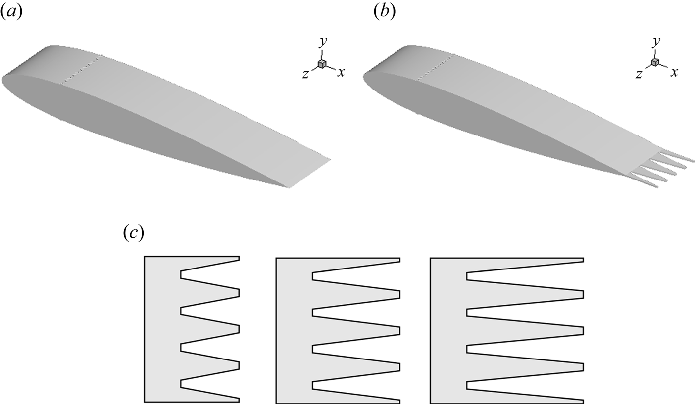
 $\delta _{99}\simeq 0.0426$. Figure 1 shows the schematic configuration of the NACA-0012 airfoil with and without the insert-type trailing-edge serrations. Currently, two types of trailing-edge serrations are often studied. One is the cut-in-type serration, which is often found in experiments (Chong et al. Reference Chong, Joseph, Vathylakis and Gruber2011; Moreau et al. Reference Moreau, Brooks and Doolan2012; Moreau & Doolan Reference Moreau and Doolan2013; Chong & Vathylakis Reference Chong and Vathylakis2015). Even though the cut-in serrations can reduce noise in the far field, they may also cause external tonal noise and aerodynamic deficit (Ji et al. Reference Ji, Qiao, Tong, Xu and Chen2014; Qiao et al. Reference Qiao, Ji, Tong, Chen and Xu2014). The other one is the insert-type serration, which is also effective in noise reduction (Gruber, Azarpeyvand & Joseph Reference Gruber, Azarpeyvand and Joseph2010a; Gruber, Joseph & Chong Reference Gruber, Joseph and Chong2010b, Reference Gruber, Joseph and Chong2011; Finez et al. Reference Finez, Jacob, Roger and Jondeau2011; Jones & Sandberg Reference Jones and Sandberg2012; León et al. Reference León, Merino-Martínez, Ragni, Avallone and Snellen2016b,Reference León, Ragni, Pröbsting, Scarano and Madsenc; Avallone et al. Reference Avallone, van der Velden, Ragni and Casalino2018; Gelot & Kim Reference Gelot and Kim2020). If the thickness of the serrations is controlled to be thin, the perturbation to the incoming flow in the boundary layer will be weak. Another advantage is that the configuration for insert-type serrations can be easily meshed and computed, making it a better choice for numerical simulation and it is adopted here.
Schematic diagram of NACA-0012 configuration for the numerical simulation. (a) NACA-0012 airfoil with straight trailing edge, (b) NACA-0012 airfoil with serrated trailing edge, (c) serrations with different lengths. The strip with zig-zag rough elements is installed on both sides of the airfoil.

The origin of the coordinate system is fixed at the leading edge of the airfoil, with the  $x$-axis pointing to the downstream direction,
 $y$-axis perpendicular to the chord of the airfoil and
 $z$ representing the horizontal position. For the serrated trailing-edge cases, the airfoil is modified to have a trailing-edge thickness of
 $0.005l$. Moreover, the serrations are modified to have a finite straight edge length of
 $0.01l$ at both the root and tip positions to avoid sharp corners for the convenience of numerical calculation. According to the theory of Howe (Reference Howe1991), the size of the serrations should be approximately the thickness of the boundary layer, so we choose a fixed-width
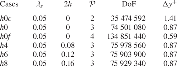
 $\lambda _s=0.05l$ and three lengths ranging from 0.08 to 0.16. The detailed parameters of serrations are given in table 1.
The computational cases and the detailed parameters ( $\lambda _s$ and
 $2h$) of the serrations. Here,
 $\mathcal {P}$ means the polynomial order used for discretization in each element. The degrees of freedom (DoF) for all computational cases are given and
 $\Delta y^{+}$ gives the maximum distance between the first collocation point and the solid wall.

The no-slip and adiabatic conditions are applied on the solid surfaces of the airfoil, and periodic boundary conditions are adopted in the spanwise direction. The far-field boundary conditions combined with the buffer zones are employed to eliminate the spurious reflections of sound. Here, the flow solver is initialized with the far-field flow conditions, namely  $\rho _0=1$,
 $U_0=0.1631$ and
 $p_0 = 0.71$. To achieve a rapid transition of the boundary layer, a strip including zig-zag rough elements is imposed on the airfoil surface at
 $x_\varDelta =0.2l$, with a height
 $h_\varDelta =0.0025l$, a chordwise extent
 $l_\varDelta =0.01l$ and a wavelength
 $\lambda _\varDelta =0.0125l$ in the spanwise direction. Each case is calculated for 450 dimensionless time units to ensure that the turbulence has been fully developed, and the last 200 dimensionless time units are used for statistical analysis (about 32 flow-through times). The pressure signal is split into three segments for frequency domain analysis, overlapping by 50 %, and a Hanning windowing is adopted. The sampling time interval for statistical and frequency analysis is
 $\Delta t = 0.01l/c_0$.
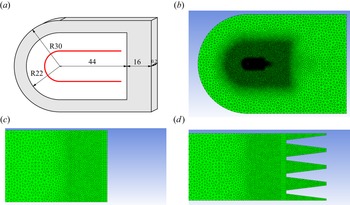
Figure 2 shows a sketch of the computational domain and an enlarged view of the unstructured mesh for the straight trailing-edge case  $h0$ and the serrated trailing-edge case
 $h6$. The computational domain consists of a semicircle with a radius of
 $30l$ in the front and a rectangle with a length of
 $60l$, and the spanwise width is
 $D=0.2l$. On the airfoil, the grid points are concentrated near the trip zone and the trailing edges. In the far field, the buffer zones are indicated by shadowed areas in figure 2(a). The minimum wall distance
 $\Delta y^{+}$ of the collocation point is less than 1 to fully resolve the viscous layer, as given in table 1.
Computational mesh for straight and serrated trailing edges. (a) The topology of the computational zone, with the buffer zone (shaded area) and the FW-H integration face (indicated by the red line). (b) Global view of the unstructured mesh. (c) The mesh near the straight trailing edge. (d) The mesh near the serrrated trailing edges.

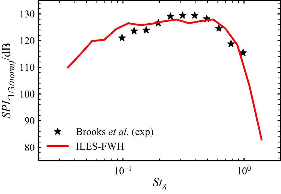
For validation purposes, we first calculated the far-field noise by the FW-H acoustic analogy (Najafi-Yazdi et al. Reference Najafi-Yazdi, Brès and Mongeau2011), which is compared with the experimental results of Brooks et al. (Reference Brooks, Pope and Marcolini1989). Figure 3 shows the normalized sound pressure level (SPL) in 1/3 octave band, which is a distance  $48.03l$ away from and top of the midpoint of the trailing edge. Both numerical and experimental results show that the SPLs will first increase and then decrease as the frequency increases. The qualitative trends of the two are relatively close, and the difference is minor when the Strouhal number
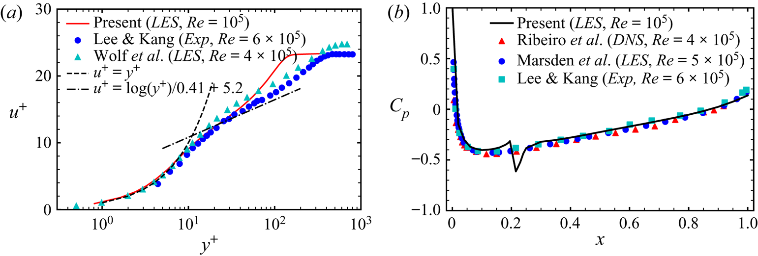
 $St_\delta$ is greater than 0.2, which we think may be attributed to the different methodologies of turbulence tripping. In the experiments, boundary layer transition was achieved by a random distribution of grit in strips, while the zig-zag type of rough elements in a strip is utilized for tripping in this study to save computational costs. In the simulations of Wolf et al. (Reference Wolf, Azevedo and Lele2012), it is also found that the way of tripping plays an essential role in generating far-field noise. Figure 4(a) shows the validation of the local flow characteristics for the straight trailing edge. We compared the boundary layer profiles between simulations and experiments at
 $x/l=0.92$. Before
 $y^{+}$ approaches 70, the curves are in good agreement. The slight deviation beyond
 $y^{+} = 70$ may be attributed to the different Reynolds numbers and the tripping method. The static pressure coefficient on the airfoil surface, shown in figure 4(b), compares well with previous experimental and numerical results.
Comparison of the sound spectrum for the straight trailing edge. The sound pressure levels are shown in normalized third-octave bands between present computational and experimental results, where the monitor point is located at the position  $R_s=48.03, \theta _s=90^{\circ }$ with the origin at the midpoint of the trailing edge. The turbulent boundary layer thickness in the current simulation at
 $x=1.0$ is
 $\delta _{99}/L \simeq 0.0426$ and 0.0753 in the experiment (Brooks, Pope & Marcolini Reference Brooks, Pope and Marcolini1989).

Comparison of the flow characteristics for the straight trailing edge. (a) Turbulent boundary layer profile at  $x=0.92$ (Lee & Kang Reference Lee and Kang2000; Wolf, Azevedo & Lele Reference Wolf, Azevedo and Lele2012). (b) The distribution of the static pressure coefficient on the airfoil surface (Lee & Kang Reference Lee and Kang2000; Marsden, Bogey & Bailly Reference Marsden, Bogey and Bailly2006; Ribeiro et al. Reference Ribeiro, Casalino, Fares and Choudhari2016).

In addition, three computational cases with the straight trailing edge, namely the coarse case  $h0c$ with fewer DoF, the normal case
 $h0$ with normal DoF and the finer case
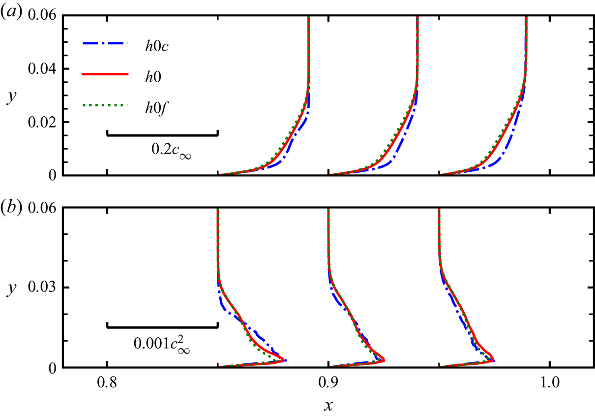
 $h0f$ with more DoF, are performed to verify the convergence of numerical solutions. Figure 5 shows the boundary layer profiles of the mean streamwise velocity
 $\langle u\rangle$ and the Reynolds stress component
 $\langle u^{\prime } u^{\prime } \rangle$ near the trailing edge for these three cases. At the three different streamwise positions, the velocity profile for the case
 $h0c$ deviates from the others to some extent at the near-wall locations, while the cases
 $h0$ and
 $h0f$ show little difference. For the Reynolds stress component
 $\langle u^{\prime } u^{\prime } \rangle$, all three cases predict the peaks well, but
 $h0c$ cannot predict the distribution correctly. Hence, by comparing the results of case
 $h0$ and case
 $h0f$, it is found that utilizing the mesh used in case
 $h0$ is enough to give almost mesh-independent solutions. The total DoF in case
 $h0$ is over 70 million, while the DoF is slightly higher for serrated cases, as given in table 1.
The velocity profiles and Reynolds stress components in the boundary layer of the airfoil. (a) Shows the streamwise velocity profile  $\langle u\rangle$ at
 $x = 0.85, 0.9, 0.95$ and (b) shows the Reynolds stress component
 $\langle u^{\prime } u^{\prime } \rangle$.

3. Results and discussion
3.1. Noise reduction due to trailing-edge serrations
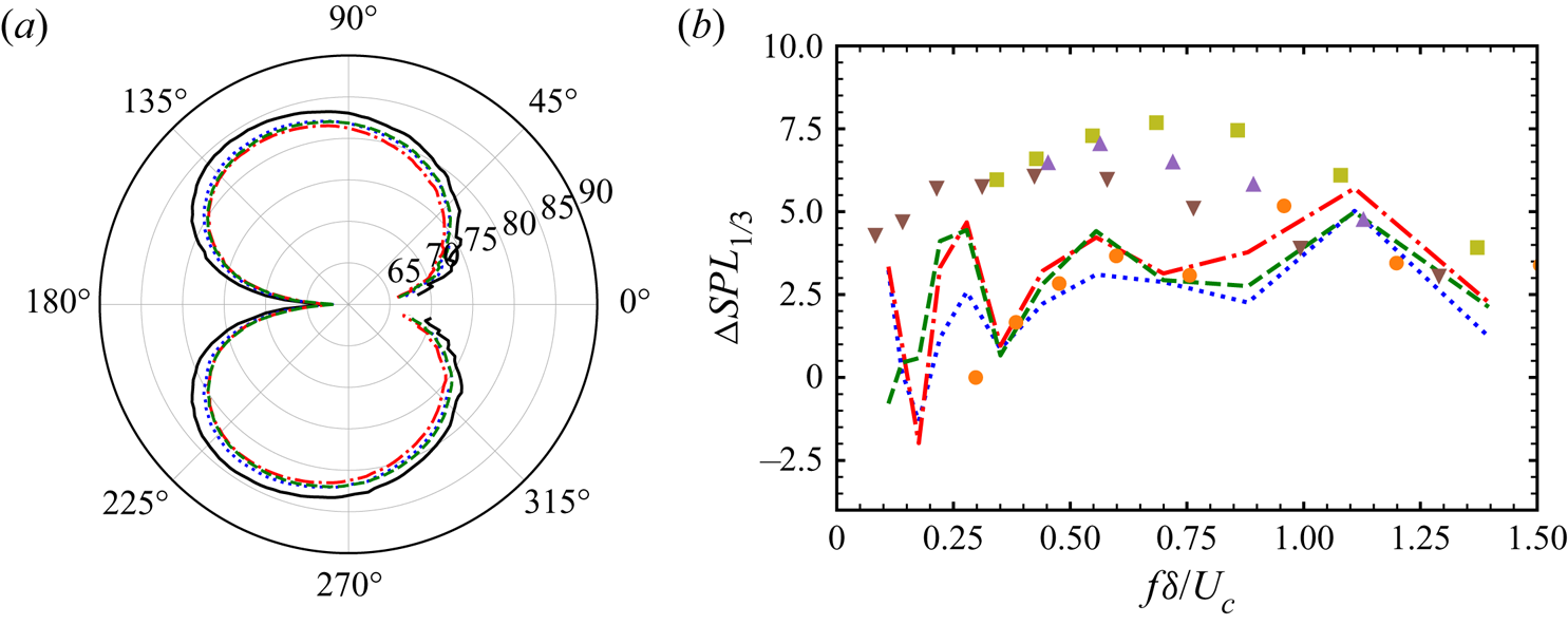
Figure 6(a) shows the OASPL directivity, computed at radius  $R_s=10l$ and polar angle
 $\theta _s=90^{\circ }$. It is seen that the noise radiated by all airfoils with serrations is reduced at almost all polar angles, with a maximum noise reduction of approximately 2 dB in OASPL. Among the serrated cases, the most effective noise reduction is found in case
 $h6$, corresponding to a length of serration
 $2h=0.12l$, in which the maximum reduction of OASPL is approximately 2.4 dB. In the present serrated cases, the noise reduction performance of case
 $h6$ with a medium length of serration is the best, which seems to be somewhat different from previous conclusions that the sharper serrations may reduce noise more (Howe Reference Howe1991; Gruber Reference Gruber2012; Chong & Vathylakis Reference Chong and Vathylakis2015; Lyu et al. Reference Lyu, Azarpeyvand and Sinayoko2016; Huang Reference Huang2017; Ayton Reference Ayton2018). For all cases, the sound generated by airfoils mainly propagates forward. The polar curves show the maximum value of OASPL occurs at a polar angle of approximately
 $\theta _s \simeq 120^{\circ }$ relative to the
 $x$-axis, with its minimum value at approximately
 $\theta _s \simeq 180^{\circ }$. The most effective noise reduction appears in the range of
 $\theta _s \in [150^{\circ }, 170^{\circ } ]$. Figure 6(b) shows the noise reduction in
 $SPL_{1/3}$ vs Strouhal number (
 $St_\delta =f\delta /U_c$), computed at radius
 $R_s=10l, \theta _s = 90^{\circ }$ about the trailing edge in the middle plane. It is seen that all the serrated cases in this study show the effect of noise reduction in the frequency range of
 $St_\delta >0.2$. Furthermore, the moderate serrated case
 $h6$ generally shows the best performance for noise reduction. The maximum noise is reduced by approximately 5 dB at
 $St_\delta \simeq 1.1$. We also compared the present results with those of previous studies (Ji et al. Reference Ji, Qiao, Tong, Xu and Chen2014; León et al. Reference León, Avallone, Pröbsting and Ragni2016a; van der Velden & Oerlemans Reference van der Velden and Oerlemans2017; Avallone et al. Reference Avallone, van der Velden, Ragni and Casalino2018). It is clear that the serration seems to be an effective means of noise reduction in a relatively broad range, even though the airfoil geometry, serration shape, tripping method, angle of attack, Mach number and Reynolds number in these cases are different.
(a) OASPL directivity shown in polar coordinates, computed at radius  $R_s=10l$ about the airfoil trailing edge and averaged in the spanwise direction, showing the straight and different serrated trailing-edge cases. (b) Comparison of the noise reduction in
 $SPL_{1/3}$ for different serrated cases. The convection velocity
 $U_c$ is estimated as
 $U_c=0.7U_0$. The positive values are for noise reduction, and negative values for noise increase:
 $\cdot \cdot \cdot$ (blue)
 $h4$,
 $2h/\delta =1.88$;
 $-\cdot -\cdot$ (red)
 $h6$,
 $2h/\delta =2.82$;
 $---$ (green)
 $h8$,
 $2h/\delta =3.76$;
 $\bullet$ (orange), Ji et al. (Reference Ji, Qiao, Tong, Xu and Chen2014), SD 2030 airfoil,
 $2h/\delta =2.87$,
 $Re_l=3.1\times 10^{5}$;
 $\blacksquare$ (green), León et al. (Reference León, Avallone, Pröbsting and Ragni2016a), NACA 0018 airfoil,
 $2h/\delta =2.92$,
 $Re_l=5.2\times 10^{5}$;
 $\blacktriangle$ (brown), van der Velden & Oerlemans (Reference van der Velden and Oerlemans2017), NACA 0018 airfoil,
 $2h/\delta =4.21$,
 $Re_l=2.8\times 10^{5}$;
 $\blacktriangledown$ (purple), Avallone et al. (Reference Avallone, van der Velden, Ragni and Casalino2018), NACA 0018 airfoil,
 $2h/\delta =4.21$,
 $Re_l=2.8\times 10^{5}$. The boundary layer thickness for the straight trailing-edge case is estimated (Griffin et al. Reference Griffin, Fu and Moin2021) to be
 $\delta /L=0.0426$, which is also used to non-dimensionalize the frequency for the serrated cases.

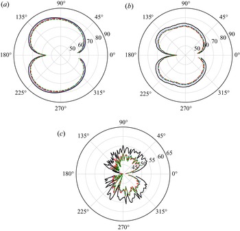
To further quantify the noise reduction for different cases, figure 7 shows acoustic power vs polar angle for various frequency bands. As shown in figure 7(a), in the low-frequency range, the compact dipole sources near the trailing edges play dominant roles in generating sound, which mainly propagates in the upstream direction relative to the  $x$-axis. Thus, the serrations do not change the main direction of propagation across all frequency ranges, but the acoustic power decreases. Different from the OASPL shown in figure 6(a), the case
 $h8$ seems to reduce more noise in this interval than case
 $h4$ and case
 $h6$, although the difference between case
 $h6$ and case
 $h8$ is relatively small. However, with increasing
 $St$, the radiated noise begins to show some non-compact characteristics, and has two lobes in the directions of polar angles
 $90^{\circ }$ and
 $140^{\circ }$. All the serrations selected reduce more noise than in the low-frequency range, and case
 $h6$ exhibits the best performance. In the high-frequency range, the values of acoustic power vary considerably with the polar angle. The serrations can significantly reduce values of acoustic power in all the frequency bands studied, and interestingly, the difference is relatively small for all serrated cases. Previously, some authors (Gruber et al. Reference Gruber, Azarpeyvand and Joseph2010a,Reference Gruber, Joseph and Chongb; Finez et al. Reference Finez, Jacob, Roger and Jondeau2011; Gruber Reference Gruber2012; Ji et al. Reference Ji, Qiao, Tong, Xu and Chen2014) found that the noise with trailing-edge serrations may increase with increasing frequency once beyond a critical frequency. This frequency, non-dimensionalized by the boundary layer thickness
 $\delta$ and convection velocity
 $U_c$, is estimated to be
 $St_\delta \approx$1 (Gruber et al. Reference Gruber, Azarpeyvand and Joseph2010a,Reference Gruber, Joseph and Chongb; Gruber Reference Gruber2012), 1.2 (Finez et al. Reference Finez, Jacob, Roger and Jondeau2011) or 1.27 (Ji et al. Reference Ji, Qiao, Tong, Xu and Chen2014). Here, all serrated cases have lower acoustic power in the range of
 $14\le St \le 20$, as shown in figure 7(c). The highest-frequency component
 $St=20$ corresponds to
 $St_\delta \approx 1.2$, which is near or below the critical values predicted by others (Finez et al. Reference Finez, Jacob, Roger and Jondeau2011; Ji et al. Reference Ji, Qiao, Tong, Xu and Chen2014). For higher-frequency components, we find the noise is much more influenced by the turbulence tripping due to the zig-zag type of rough elements, which are not considered in this study.
Acoustic power directivity for the straight and serrated trailing edges in polar coordinates, computed at radius  $R_s=10l$ and averaged in the spanwise direction and in different frequency ranges; (a)
 $2\le St\le 6$, (b)
 $6\le St\le 14$, (c)
 $14\le St\le 20$: —— (black)
 $h0$;
 $\cdots \cdots$ (blue)
 $h4$;
 $-\cdot -\cdot$ (red)
 $h6$;
 $---$ (green)
 $h8$.

3.2. The influence of serrations on local flow structures
As previously mentioned, the noise generation is weakened by trailing-edge serrations, which is inevitably related to the change of flow structures. In this subsection, we are devoted to studying the influence of serrations on general flow structures. Since the noise reduction in case  $h6$ is the best, we particularly compare the results of case
 $h0$ and case
 $h6$. Figure 8 shows the isocontours of the second invariant of the velocity gradient (
 $Q$) and the dilatation rate in the middle plane for case
 $h0$ and case
 $h6$. The
 $Q$ value can be used to isolate the flow region where vorticity prevails over the strain rate, and it is defined as
 $Q = \frac {1}{2}(\|\boldsymbol {\varOmega }\|^{2}-\|\boldsymbol {D}\|^{2}) = -\frac {1}{2}u_{i,j}u_{j,i}$, where
 $\boldsymbol {\varOmega }$ is the strain rate tensor and
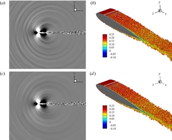
 $\boldsymbol {D}$ the vorticity tensor. As shown in figures 8(b) and 8(d), before the tripping position at
 $x=0.2l$, the flows are all laminar, with smooth velocity change over the airfoil surface. After the tripping position, the flow is destabilized, causing the formation of a Tollmien–Schlichting wave, which further develops into three-dimensional random turbulent flow structures. The scale of such flow structures will become larger along the downstream direction, similar to fully developed boundary layers. There is little visual difference in vortex structures between case
 $h0$ and case
 $h6$. However, from the dilatation fields shown in figures 8(a) and 8(c), the attenuation of the intensities of acoustic waves can be observed. Moreover, it can be inferred from the wave patterns that the source of noise scattering is mainly located near the trailing edge.
The pattern of sound propagation and vortex structures for (a,b) case  $h0$ and (c,d) case
 $h6$. (a,c) The dilatation rate over the range
 $\boldsymbol{\nabla} \cdot \boldsymbol {u} \in [-0.0004, 0.0004]$. (b,d) Vortex structures shown by the
 $Q$-criterion, in which
 $Q=1$ coloured by streamwise velocity.

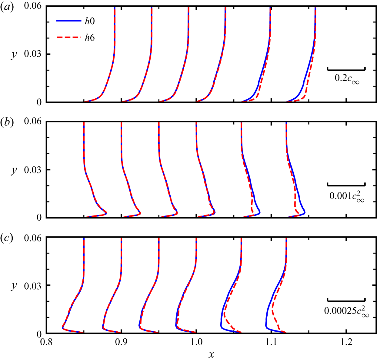
Next, special attention is paid to study the flow characteristics of the boundary layer near the trailing edge. Figure 9 shows the mean velocity profiles of  $\langle u \rangle$ and Reynolds stress components of
 $\langle u'u' \rangle$ and
 $\langle u^{\prime } v^{\prime } \rangle$ in the middle vertical plane of case
 $h0$ and case
 $h6$ at the positions of
 $x/l$=0.85, 0.9, 0.95, 1.0, 1.06 and 1.12. The thickness of the boundary layer
 $\delta$ plays an essential role in Howe's noise scattering model (Howe Reference Howe1991), which mainly determines the critical non-dimensional frequency
 $\omega \delta /U_c$, over which noise reduction is independent of frequency (Gruber Reference Gruber2012; Azarpeyvand, Gruber & Joseph Reference Azarpeyvand, Gruber and Joseph2013). On the surface of the airfoil (
 $x< l$), the thickness of the boundary layer grows along the streamwise direction, and there are little differences in mean profiles
 $\langle u \rangle$, as well as the Reynolds stress profiles of
 $\langle u'u' \rangle$ and
 $\langle v'v' \rangle$, in case
 $h0$ and case
 $h6$. However, in case
 $h6$, the boundary layer becomes thinner on the serration surface, as indicated by the velocity profiles, due to the positive streamwise pressure gradient. Additionally, the intensities of the Reynolds stresses are weakened because of the local flow acceleration. From the comparison of general turbulent quantities in cases
 $h0$ and
 $h6$, we find that the influences of serrations on the upstream velocity-related statistics (
 $x< l$) are relatively small (Sandberg & Jones Reference Sandberg and Jones2011; Jones & Sandberg Reference Jones and Sandberg2012).
Velocity profiles and the Reynolds stress components for straight ( $h0$) and serrated trailing-edge case
 $h6$ in the boundary layer in the middle vertical plane. The profiles of (a)
 $\langle u\rangle$, (b)
 $\langle u^{\prime } u^{\prime } \rangle$ and (c)
 $\langle u^{\prime } v^{\prime } \rangle$, at the positions of
 $x/l$=0.85, 0.9, 0.95, 1.0, 1.06 and 1.12, respectively. For comparison purposes, the profile in case
 $h0$ at
 $x=l$ is extended to the positions
 $x/l>1$, where no solid surface exists.

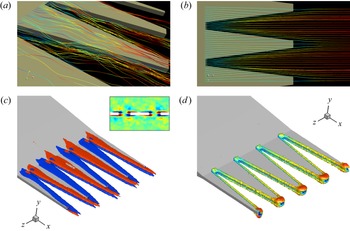
Figures 10(a) and 10(b) show the instantaneous and averaged streamlines near the serrations. The streamlines are extracted with the seed lines locating at  $x/l=1$,
 $z/l=\pm 0.005$. There is a low-speed flow near the roots and a high-speed flow close to the tips between the serrations due to the turbulence mixing process. On both sides of the serration, the streamlines are intertwined, which implies the existence of side vortices. From the time-averaged results, it is seen that the streamlines first deflect to the serrated gap and undergo an acceleration process near the roots. Then, as the cross-sectional area of the gap increases, the flow begins to expand and deflect towards the serrated direction near the tips. Understanding this change of fluid motion is helpful to establish noise prediction models, especially since the existing models usually assume a uniform flow that deviates from the actual situation. Figure 10(c) shows the isocontours of mean vorticity for the case
 $h6$ near the serrated trailing edges. We can observe that the vortex pairs are formed, concentrating near the side edges of the serrations. Due to the chamfered ends, the side vortex will extend some distance downstream in the wake. From the mean streamwise vorticity, there are vorticities of opposite signs above and below the serrated trailing edge caused by the local transverse flow. Specifically, the flow above and below the serrations deviate from the centreline and flow towards the gap region, then shear with the low-speed flow near the serration edges and form the vorticities of opposite signs. The two vortices, one on the top and one on the bottom, are further shown by the
 $Q$ criterion with the iso-surface of
 $Q=1$ in figure 10(d). Previously, Chong & Vathylakis (Reference Chong and Vathylakis2015) also identified the existence of the pressure-driven, oblique vortical structures near the sawtooth edges in plate experiments. Avallone et al. (Reference Avallone, Pröbsting and Ragni2016) found the streamwise-oriented and counter-rotating vortices to be the main features for the mean flow field, which can affect the effective angle experienced by the turbulent flow and finally leads to the noise reduction, as pointed out in Howe (Reference Howe1991). Similar descriptions of the vortex structures can also be found in some studies (Chong et al. Reference Chong, Joseph, Vathylakis and Gruber2011; Qiao et al. Reference Qiao, Ji, Tong, Chen and Xu2014; León et al. Reference León, Ragni, Pröbsting, Scarano and Madsen2016c).
Flow structures near the serrations. (a) The instantaneous streamlines near the trailing edges. (b) The mean streamlines near the trailing edges. (c) The iso-surfaces of mean vorticity  $\omega _x=\pm 1.5$ and (d) the iso-surface of
 $Q=1$ for serrated trailing-edge case
 $h6$ are also shown. The slice show in (c) is extracted at
 $x=1.04$.

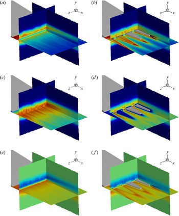
Figure 11 shows the spatial distributions of different components of the Reynolds stress tensor near the trailing edges. It is clear that the Reynolds stresses have been changed significantly. In figure 11(a), in the near wake in case  $h0$, two peaks of
 $\langle u^{\prime } u^{\prime }\rangle$ can be found at a distance above and below the
 $y=0$ plane. For case
 $h6$, the serrations also serve as important sources for inducing Reynolds stresses. The larger values of
 $\langle u^{\prime } u^{\prime }\rangle$ appear in the boundary layers of the serrated edges, as seen in figure 11(b). The effect of serrations on
 $\langle v^{\prime } v^{\prime }\rangle$ seems to be quite different. For case
 $h0$, the intensity of
 $\langle v^{\prime } v^{\prime }\rangle$ in the near wake is strong. However, due to the blocking effect of serrated edges, the intensity of
 $\langle v^{\prime } v^{\prime }\rangle$ in the boundary layer of serrated edges is relatively weak. The peaks of
 $\langle v^{\prime } v^{\prime }\rangle$ occur in the gap in case
 $h6$. Also,
 $\langle v^{\prime } v^{\prime }\rangle$ in case
 $h6$ is weakened compared with that in case
 $h0$. In case
 $h0$, the shear stress
 $\langle u^{\prime } v^{\prime }\rangle$ also concentrates near the wall surface and has the opposite sign for different sides of the airfoil. However, for case
 $h6$,
 $\langle u^{\prime } v^{\prime }\rangle$ concentrates mainly near the side edges of serrations, which is consistent with the distribution of the side vortex pairs. Generally, the serrations strengthen the streamwise fluctuations while weakening the fluctuation in the normal direction. In addition, the enhanced shear stress near the serrations can be observed, which is due to the existence of the side vortex pairs.
The spatial distributions of Reynolds stress components for the straight case ( $h0$) and serrated case (
 $h6$). (a,c,e) Show
 $\langle u^{\prime } u^{\prime }\rangle$ (range 0
 $\sim 5\times 10^{-4}$),
 $\langle v^{\prime } v^{\prime }\rangle$ (range
 $0\sim 2.5\times 10^{-4}$) and
 $\langle u^{\prime } v^{\prime }\rangle$ (range
 $\pm 3\times 10^{-4}$) for case
 $h0$, and (b,d,f) are for case
 $h6$. The slices in the panels are located in three fixed planes, namely the
 $y$–
 $z$ plane
 $x=1.04$,
 $x$–
 $z$ plane
 $y=-0.005$ and
 $x$–
 $y$ plane
 $z = -0.05$. For easy comparison, the solid serrations in (b,d,f) are partly removed to demonstrate clearly the distribution of the Reynolds stress components.

3.3. Dynamic mode decomposition of near-field pressure
In the above subsection, we have found that serrations mainly influence the local flow structures. Next, we are devoted to investigating the effects of serrations on a non-local quantity, i.e. the pressure. Dynamic mode decomposition (DMD) (Schmid Reference Schmid2010) is employed to analyse the unsteady fluctuating pressure fields. Given a collection of the continuous snapshots of the pressure field, with time interval  $\Delta t$
 \begin{equation} \boldsymbol{P_1^{N}}=\{\boldsymbol{p}_1, \boldsymbol{p}_2, \boldsymbol{p}_3, \ldots, \boldsymbol{p}_N\}. \end{equation}
We assume that the pressure field  $\boldsymbol {p}_i$ is related to the subsequent flow field
 $\boldsymbol {p}_{i+1}$ by a linear mapping operator
 $\boldsymbol {A}$, which describes the dynamic characteristics for the system. Specifically, the relation reads
 \begin{equation} \boldsymbol{p}_{i+1}=\boldsymbol{A}\boldsymbol{p}_i. \end{equation}
Beyond a large critical number of snapshots, the further flow field  $\boldsymbol {p}_N$ can be expressed as the linear combination of the previous, and linearly independent vectors
 $\boldsymbol {p}_i$,
 $i$=1,
 $\ldots$,
 $N-1$, namely
 \begin{equation} \boldsymbol{p}_N=a_1\boldsymbol{p}_1+a_2\boldsymbol{p}_2+ \cdots+a_{N-1}\boldsymbol{p}_{N-1}+\boldsymbol{r}. \end{equation}
So the mapping relation can be rearranged as
 \begin{equation} \{\boldsymbol{p}_2, \boldsymbol{p}_3, \ldots, \boldsymbol{p}_{N}\} =\boldsymbol{A}\{\boldsymbol{p}_1, \boldsymbol{p}_2, \ldots, \boldsymbol{p}_{N-1}\} =\{\boldsymbol{p}_2, \boldsymbol{p}_3, \ldots, \boldsymbol{P}_1^{N-1}\boldsymbol{a}\}+\boldsymbol{r} \boldsymbol{e}_{N-1}^{T}, \end{equation}
or in its equivalent matrix form
 \begin{equation} \boldsymbol{P}_2^{N}=\boldsymbol{A}\boldsymbol{P}_1^{N-1}= \boldsymbol{P}_1^{N-1}\boldsymbol{S}+\boldsymbol{r} \boldsymbol{e}_{N-1}^{T}. \end{equation}
The eigen-decomposition of the companion operator  $\boldsymbol {S}$ is defined as
 \begin{equation} \boldsymbol{Sq}=\lambda \boldsymbol{q}, \end{equation}
where  $\lambda$ means the eigenvalue and
 $\boldsymbol {q}$ the eigenvector. Then, the eigen-frequency can be calculated as
 $f=\Im (\log (\lambda ))/(2{\rm \pi} \Delta t)$, and
 $\sum _{i=1}^{N-1}\boldsymbol {p}_i q_i$ gives the spatial distribution of the mode at the corresponding frequency. Moreover, the mode energy is defined as the Euclidean norm, or the
 $L_2$-norm, of the mode vector. The calculation of the companion operator
 $\boldsymbol {S}$ is usually conducted with the QR (orthogonal-triangular decomposition) or SVD (singular value decomposition) algorithm, and more details can be found in Schmid et al. (Reference Schmid, Li, Juniper and Pust2011). Currently, 500 snapshots of pressure fluctuations in the near field, namely the subdomain
 $[-0.5, 2.5] \times [-0.5, 0.5] \times [-0.1, 0.1]$, are utilized for mode analysis, with the constant time interval
 $\Delta t = 0.1l/c_0$.
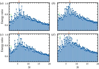
Figure 12 illustrates the distribution of the DMD mode energy in the frequency domain, where its maximum value has been used to normalize the mode energy for each case. It is observed that all the cases have their peaks in a narrow frequency range of  $St \simeq 5 \sim 7$, which should correspond to the most convectively amplified hydrodynamic instability waves. For case
 $h6$, suppose the convection velocity is evaluated as
 $U_c=0.7U_0$, and then the characteristic spatial scale corresponding to the peak frequency is approximately
 $\lambda _{ch}=U_c/f\simeq 0.12l$, which is close to the streamwise wavelength of the large-scale mode structures. Another interesting finding is that case
 $h6$ seems to have a similar energy distribution to the straight trailing-edge case, which may be attributed to the fact that the convection processes of the detached vortices are less affected when the serration length was close to the characteristic spatial scale, i.e.
 $2h\approx \lambda _{ch}$. In case
 $h6$, the energy distribution of most modes is slightly lower than that of other serrated cases but still higher than that of the straight trailing-edge case. In general, mode energy decays rapidly away from these peaks. For most dynamic modes, the energy ratios in serrated cases tend to be higher, which means that the mode energy of pressure will transfer from the most energy-containing modes to other modes within a wide range of frequencies. The redistribution of mode energy will inevitably affect the far-field noise reduction performance. Here, we choose two typical frequencies for analysis of mode structures for all cases, namely
 $St\simeq 6$ and
 $St\simeq 2$. The frequency
 $St\simeq 6$ is related to the highest energy ratio and also the most amplified instability wave. The mode near
 $St\simeq 2$, representing the large-scale structures, is selected.
The distribution of the mode energy ratio in the frequency domain for straight and serrated trailing-edge cases with dynamic mode decomposition algorithms. (a) Shows straight trailing edges, and (b–d) are for serrated trailing edges, namely case  $h4$,
 $h6$ and
 $h8$, respectively. The red arrows point to the global peaks across the frequency domain, namely 5.64, 6.87, 5.40 and 6.38 for each case, and the green arrows to the local peaks near
 $St\simeq 2$, namely 1.96, 1.84, 1.96 and 2.21, which are selected for further investigation.

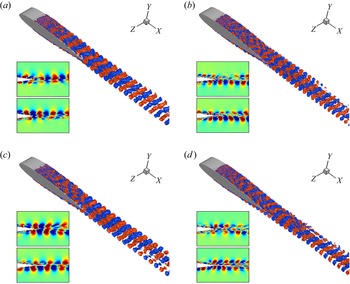
Figure 13 shows the isocontours of the most energetic mode near the frequency  $St\simeq 6$. After the tripping strip, the transition process can be clearly observed. Near the trailing edges, it is seen that the flow structure will develop into larger scales. In the near wake, the flow structure will keep its shape for a short distance, approximately
 $0.5l$ away from the trailing edges, then shrink and decay. It is remarkable that the serrations affect the mode structures near the upstream airfoil surface. With the serrations, the mode structure on the airfoil surface shows a less coherent, distorted behaviour in the spanwise direction and also near the serrations. This is also expressed in the phase differences shown in the panels. As mentioned before, we have shown that the serrations have little effect on the upstream velocity fields due to the fact that the vortex perturbation will convect to the downstream position. In contrast, due to the non-local feature of the pressure (Kim Reference Kim1989), the pressure perturbation near the trailing edges will propagate to the whole flow field, especially the upstream positions. Figure 14 shows the mode structures at the frequency
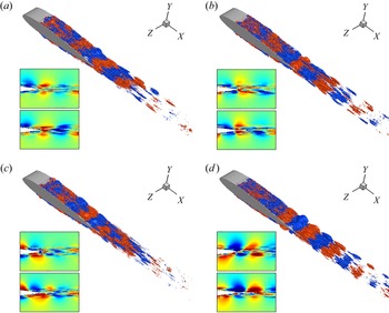
 $St \simeq 2$. Such a frequency corresponds to the scale of the spanwise size of the computational domain, which is less affected by the serrations because of a large difference in scale. In the near wake, the case
 $h8$ shows a greater coherence level in the spanwise direction near the trailing edge, which corresponds to steeper peaks than the other cases in the energy ratio distribution and may be attributed to more coherent detached vortices. For this low frequency,
 $St \approx 2$, the mode structures would be more influenced by the potential flow than the turbulent vortices. Thus, we suggest the reason might be that the change of potential flow characteristics will be more obvious in case
 $h8$ with relatively long serrations, and the longer serrations could cause a more substantial influence on the vortices in the wake. In addition, in the wake region, the long wave structure seems to decay faster than the short wave structure, compared with that in figure 13.
Iso-contours of the most energetic mode structures near  $St\simeq 6$, namely 5.64, 6.87, 5.40 and 6.38 for difference cases. (a) Shows straight trailing edges (
 $h0$), and (b–d) are for serrated cases
 $h4$,
 $h6$ and
 $h8$, respectively. In each panel, the upper view of the slice is extracted at
 $z=-0.025$ (root location for the serrated cases) and the lower slice at
 $z=0$ (tip location for the serrated cases).

Iso-contours of the mode structures with local energy peaks around  $St\simeq 2$, namely 1.96, 1.84, 1.96 and 2.21 for different cases. (a) Shows straight trailing edges (
 $h0$), and (b–d) are for serrated cases
 $h4$,
 $h6$ and
 $h8$, respectively. In each panel, the upper view of the slice is extracted at
 $z=-0.025$ (root location for the serrated cases) and the lower view at
 $z=0$ (tip location for the serrated cases).

3.4. The influence of serrations on dipole sources
As stated in (2.6), the FW-H acoustic analogy can split the noise sources into thickness, loading and quadrupole sources. When the wall has no relative motion and the velocity at the wall is zero, only the dipole source needs to be considered on the airfoil surface. The strengths of dipole sources measured by OASPL for the straight and all serrated cases are shown in figure 15. For case  $h0$, it is seen that the noise intensity changes smoothly near the trailing edges. While for the serrated cases, the intensity of the dipole source increases suddenly at the root of the serrations and then decreases gradually. The intensity of the dipole source at the tip is the weakest. These findings are consistent with the previous studies (Chong & Vathylakis Reference Chong and Vathylakis2015; Avallone et al. Reference Avallone, van der Velden, Ragni and Casalino2018). The high-intensity dipole source near the root is caused by the discontinuous change of geometry. It is also worth noting that the distribution of noise sources is very similar in all cases of serration. The high-intensity source (the red area) is located in the position range of
 $1\lesssim x/l \lesssim 1.02$, the medium-intensity source (the yellow area) is located in the range of
 $1.02\lesssim x/l \lesssim 1.08$ and the lower-intensity source (the cyan area) is located in the range of
 $x/l \gtrsim 1.08$. It can be inferred that the similar noise distribution is mainly caused by the similar upstream boundary layers, as discussed previously.
The dipole source strengths for straight and serrated trailing edges, which are indicated by OASPL. (a) Shows straight trailing-edge case  $h0$, and (b
 $-$d) serrated trailing edges, namely
 $h4$,
 $h6$ and
 $h8$, respectively.

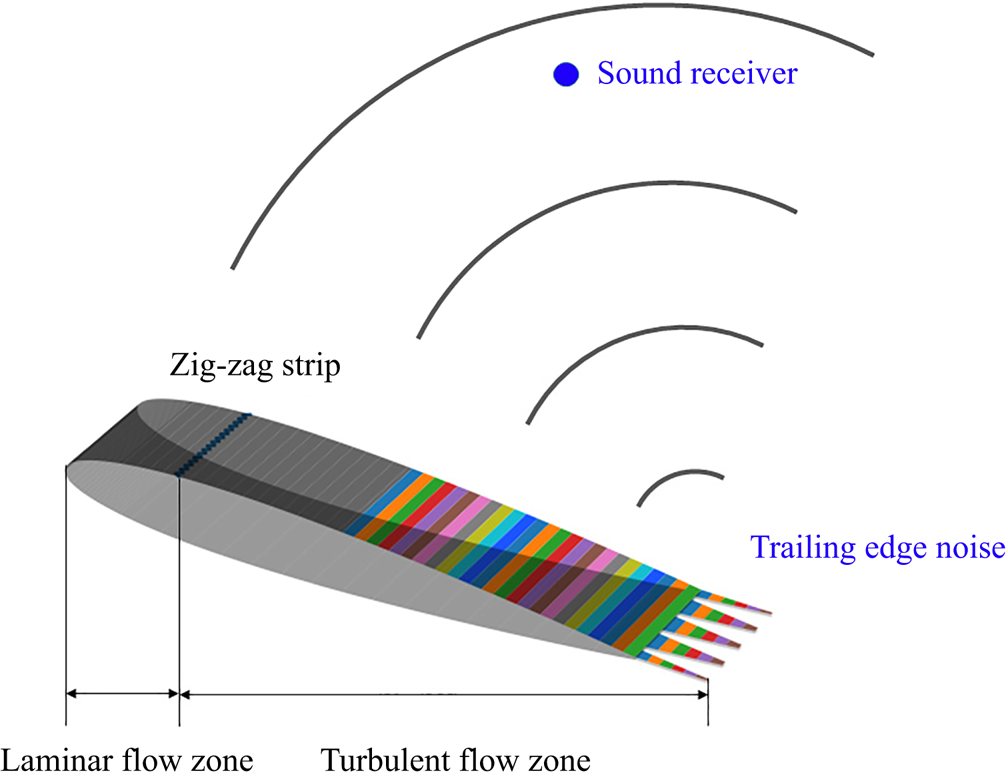
It has been shown that the most vital noise sources are mainly located near the trailing edges. In order to study the detailed distribution of the noise sources on the airfoil and its influence on the far-field noise, we divide the airfoil surface, including the serrated surface, into many strips (Avallone et al. Reference Avallone, van der Velden, Ragni and Casalino2018; Teruna et al. Reference Teruna, Manegar, Avallone, Ragni, Casalino and Carolus2020), as illustrated in figure 16. Here, we are mainly concerned with the influence of a fully developed area, and the surface with  $x/l>0.5$ is split into many spanwise strips. For serrated trailing edges, the strips with
 $x/l\le 1$ relate to the location on the airfoil surface, and the strips with
 $x/l>1$ relate to the location on the serration surface. Hence, for straight trailing edges, only the strips with
 $x/l\le 1$ are considered. In addition, the contribution of each strip to the far-field noise is obtained by integrating the dipole sources on each strip surface.
Geometric sketches of the strips for pressure coherence study. Strips are located on the wall surface with  $x/l>0.5$ for serrated trailing edges, and similar for the straight trailing edge except that the strips with
 $x/l>1$ are not considered. Specifically, every two strips have the streamwise separation
 $\Delta x=0.01$ (every other strip is shown).

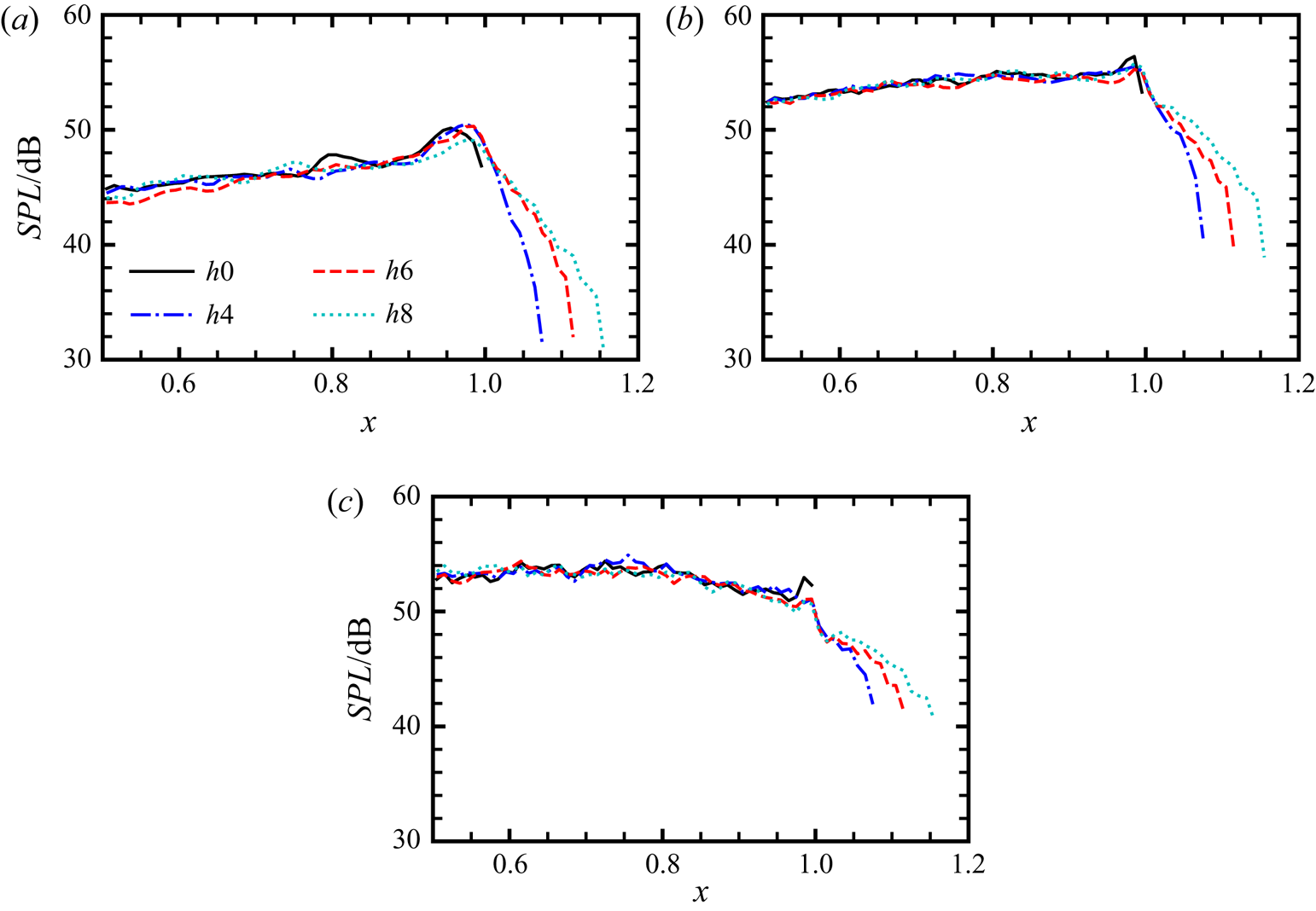
Figure 17 shows SPLs for the noise at the observer in different frequency bands, which are computed by integrating the dipole sources on each strip. The selected observer is located at  $R_s=10l, \theta _s = 90^{\circ }$ from the trailing edge in the median vertical plane. As shown in figures 17(a) and 17(b), the peak noise sources are located near the trailing edges in the frequency ranges of
 $2\le St \le 6$ and
 $6\le St \le 14$. In contrast, the most substantial noise is produced by the strips around
 $x/l=0.75$ in the high-frequency range of
 $14\le St \le 20$. For
 $2\le St \le 6$, the most significant noise sources is located around
 $x/l \approx 0.95\sim 1$. Comparing different positions, we find that the SPLs of case
 $h6$ are lower than those of other serrated cases before
 $x/l\simeq 0.7$, but the difference is less than 2 dB. In addition, case
 $h4$ has a lower amplitude in the area of
 $0.7 \lesssim x/l \lesssim 0.9$ and case
 $h8$ has a lower amplitude in the area of
 $0.9 \lesssim x/l \lesssim 1$. On the surface of serrations, due to the weakening of the noise source intensity (see also figure 15), the SPL at the observer produced by the strip from the root to tip decreases rapidly as well. Interestingly, although the serration length is different, the far-field noise level produced by the tip of the serration is very close in this frequency range. For
 $6 \le St \le 14$, it is easy to find that the primary noise sources are located near the trailing edges. In this frequency range, the SPLs at the observer produced by the strips on the airfoil surfaces in different serrated cases show little difference, except that the case
 $h6$ shows a lower peak value than other serrated cases around
 $x/l=1$. Similarly, for
 $14\le St \le 20$, the SPLs at the observer generated by the airfoil surfaces in different serrated cases are almost identical. A critical difference is that the strips of
 $0.5\lesssim x/l \lesssim 0.8$ become more important noise sources. In agreement with the DMD analysis, these findings confirm that the upstream dipole sources can also be affected by the trailing-edge serrations, which should be considered in the theoretical modelling of the sound scattering process.
The observer's SPLs at  $R_s=10l, \theta _s = 90^{\circ }$ about the trailing edge in the middle plane, produced by the sources near the trailing edges, which show the individual contributions for strips in different frequency bands. (a) Low-frequency range
 $2\le St \le 6$, (b) mid-frequency range
 $6\le St \le 14$, (c) high-frequency range
 $14\le St \le 20$.

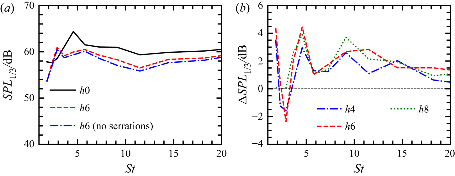
To further explore the interaction between different strips and the overall effect on the noise at the observer, we plot the  $SPL_{1/3}$ spectra of total pressure in the far field contributed by all strips. Figure 18(a) shows the comparison of
 $SPL_{1/3}$ spectra between case
 $h0$ and case
 $h6$. In case
 $h0$, it is found that the amplitude of
 $SPL_{1/3}$ first increases with increasing
 $St$, attains its peak at
 $St \approx 5$ and then decays slowly. Although there is a similar trend in case
 $h6$, the amplitudes of
 $SPL_{1/3}$ are reduced at nearly all frequencies, except at
 $St\simeq 3$, where the peak occurs. If we remove the contributions of the dipole sources on the serrations in case
 $h6$, the
 $SPL_{1/3}$ amplitudes are further reduced. This result indicates that the far-field noise reduction mainly results from dipole sources on the airfoil surface. In other words, the serrations redistribute the dipole sources on the airfoil surface, which is favourable for noise reduction. Figure 18(b) shows the comparison of the noise reduction effect with
 $\Delta SPL_{1/3}$ at the observer for all cases by integrating dipole sources on the wall surface. It is observed that the noise reduction performance of case
 $h6$ and case
 $h8$ is better than the case
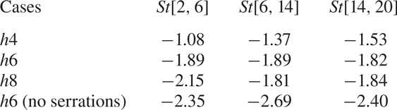
 $h4$. To be specific, the noise reduction capability in each frequency band is also computed, and listed in table 2. It is found that case
 $h8$ can reduce more noise than other serrated cases in low- and high-frequency bands, indicating that case
 $h8$ would be the best choice for noise reduction if only the dipole sources are considered. This finding is contradictory to the practical results shown in figure 6. We believe this is mainly caused by the quadrupole sources influenced by the serrations, which will be further discussed.
Value of  $SPL_{1/3}$ for the noise at an observer for
 $R_s=10l, \theta _s = 90^{\circ }$ about the trailing edge produced by the sources near the trailing edge, which shows the cumulative sum results. (a) The
 $SPL_{1/3}$ comparison between case
 $h0$ and case
 $h6$, (b) comparison between all cases, where the positive values are for noise reduction.

SPL obtained in each frequency band for the observer at  $R_s=10l, \theta _s = 90^{\circ }$ about the trailing edge in the middle plane.

Beyond the discussion on the variation of the dipole source strength, we also explore the coherence between different strips (Avallone et al. Reference Avallone, van der Velden, Ragni and Casalino2018; Teruna et al. Reference Teruna, Manegar, Avallone, Ragni, Casalino and Carolus2020, Reference Teruna, Avallone, Ragni and Casalino2021). The cross-spectrum density (CSD) between two pressure signals at two locations is defined as
 \begin{equation} c_{i,j}= \int_{-\infty}^{\infty} \left[ \int_{-\infty}^{\infty}p^{\prime}(x_i, t)p^{\prime}(x_j, t+\tau)d\tau \right] \, {\rm e}^{j\omega t}\, {{\rm d}}t. \end{equation}
The coherence refers to the normalized amplitude for the CSD, i.e.  $C_{i,j}={|c_{i,j}|}/{\sqrt {|c_{i,i}| |c_{j,j}| }}$. The cosine value of the complex angle for the CSD is adopted to show the phase difference between different signals.
For convenience, the quantity studied is averaged in each frequency band  $[f_a,f_b]$. We define the frequency-averaged quantity as
 \begin{equation} \bar\phi = \frac{1}{f_b-f_a}\int_{f_a}^{f_b}\phi(f)\, {{\rm d}}f, \end{equation}
where the integrand  $\phi (f)$ can be the coherence value or the cosine value of the phase angle, and the average symbols will be omitted in the following parts.
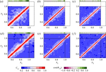
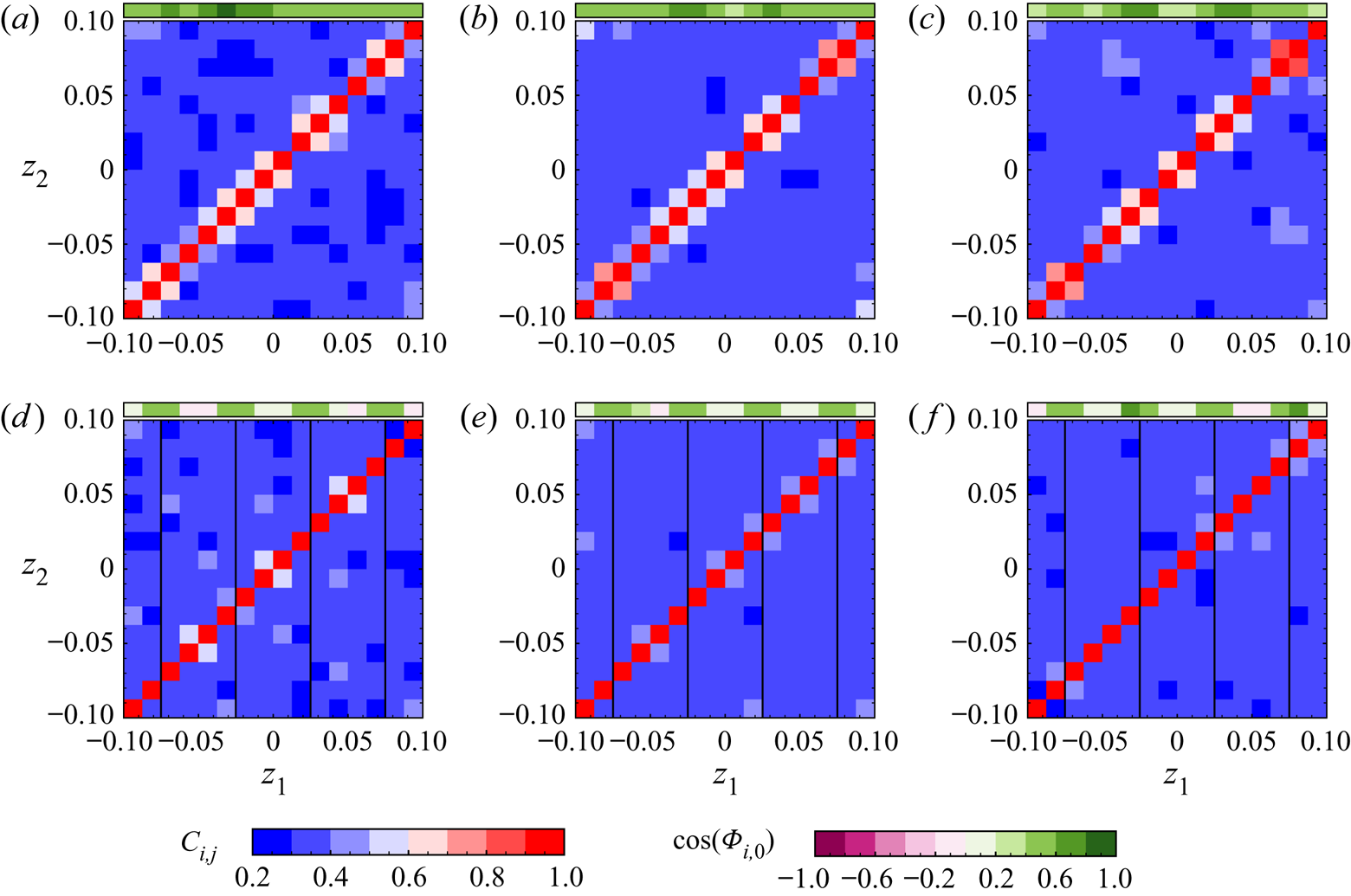
Figure 19 shows the coherence between the pressure signals at the observer computed by integrating different strips for case  $h0$ and case
 $h6$, and the cosine of the phase angle computed by integrating each strip and by integrating all strips. For
 $2\le St \le 6$, the cosines of the phase angle are almost all positive in the region of
 $0.5\le x/l \le 1$, although the serrated case
 $h6$ shows a slightly lower cosine value. The coherence for the case
 $h6$ is slightly lower than case
 $h0$ when
 $x/l \lesssim 0.9$, which indicates a shorter coherence length in the streamwise direction. The reduced coherence length and increased phase angle show the destructive interference, which usually plays an essential role in making the airfoil surface a low-efficiency noise scattering object (Avallone et al. Reference Avallone, van der Velden, Ragni and Casalino2018). In addition, near the trailing edge, the presence of serrations significantly increases the coherence but has no significant effect on the phase. However, there is an obvious phase difference between the pressure produced by the serrations and the total pressure, which also shows that the sound produced by the dipole source on the serrations is helpful to produce the effect of destructive interference so as to achieve the effect of noise reduction. Similar distribution for the phase difference and the coherence can also be found in the frequency ranges of
 $6\le St\le 14$ and
 $14\le St\le 20$, but the coherence is much lower, and the phase angle is even larger. Generally, the presence of serrations will weaken the coherence of the noise source on the airfoil surface, and the phase difference will increase. The pressure produced by the serration itself can reduce the noise by means of destructive interference.
Phase difference with respect to the whole part (purple–green scale) and coherence (blue–red scale) between different strips in the flow direction. (a  $-$c) Show straight trailing-edge case
 $h0$ with
 $St$ in [2, 6], [6, 14] and [14, 20], and (d
 $-$f) show serrated trailing-edge case
 $h6$. The analysis is based on the pressure fluctuation in the far field contributed by each strip on the wall surface. Specifically, the coherence
 $C_{i, j}$ is calculated with the strips
 $i$ and
 $j$, and the cosine value of the phase angle
 $\cos (\varPhi _{i, 0})$ is based on the individual strip
 $i$ and the whole integration surface.

Furthermore, the coherence between different spanwise strips is also studied for case  $h0$ and case
 $h6$. The spanwise strips are located in
 $1< x/l<1.02$ for serrated trailing edges and
 $0.98< x/l<1$ for straight trailing edges, with 16 strips evenly distributed in the spanwise direction. Figure 20 compares the coherence and cosine of phase angle in different frequency bands for case
 $h0$ and case
 $h6$. For
 $2\le St\le 6$, the serrations result in a lower coherence and negative cosine value for the dipole source in the serrated case. Compared with the straight trailing-edge case, we observe a lower negative value near the gap in the serrated case, and their distributions in the high-frequency region are similar. Thus, the analysis of noise sources shows that the trailing-edge serrations influence the upstream dipole sources, and also reduce far-field noise by enhancing the effect of destructive interference.
Phase difference with respect to the whole part (purple–green scale) and coherence (blue–red scale) between different strips in the spanwise direction. (a  $-$c) are for straight trailing-edge case
 $h0$ with
 $St$ in [2, 6], [6, 14] and [14, 20], and (d
 $-$f) for serrated trailing-edge case
 $h6$. The black lines in the panels show the locations of the gap between the serrations. The analysis is based on the pressure fluctuation in the far field contributed by each strip in the spanwise direction.

3.5. The influence of serrations on flow noise sources
In the above subsection, a detailed analysis has been carried out about the change of the dipole noise source on the wall surface due to serrations. Here, we further adopt (2.20) to study the change of flow noise sources in the near wake close to the trailing edge in order to give some insights into the relationship between flow structure and far-field noise. This might also explain why case  $h6$ reduces more noise practically, contradicting the pure dipole source analysis.
Presently, the flow speed is relatively low, the gradient of enthalpy is negligible and thus we only consider the term ( $-\beta$) as the noise source. For case
 $h0$ and case
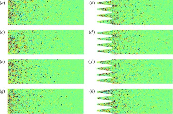
 $h6$, figure 21 shows the distributions of noise source within a typical flow cycle in the middle
 $x-z$ plane. Since the noise source decays quickly downstream, we here only show the noise sources in the near wake. Specifically, for the straight trailing edge, the strong flow noise sources are mainly concentrated within
 $0.05l$ from the trailing edge. While for serrated trailing edges, the noise sources have a wider distribution. The source is distributed along the serration edge, and the distribution seems to be scattered. These sources are closely related to the side vortex pair.
Noise source ( $-\beta$) distribution (range
 $\pm 300$) for straight and serrated trailing edges in the near-wake region of
 $x/l \in [1,1.6], z/l \in [-0.1, 0.1]$ at the
 $y/l=0$ plane. (a,c,e,g) Show case
 $h0$ in a flow cycle with
 $t = 0, T/4, T/2, 3T/4$ (
 $T=l/U_0$), and (b,d,f,h) case
 $h6$.

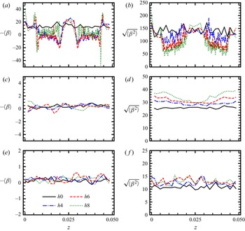
Next, we compare the intensity of the flow noise source quantitatively at some selected positions close to the trailing edge. Figure 22(a) demonstrates the distribution of the averaged noise source term  $-\langle \beta \rangle$ at a relative position of
 $x = x_{t.e.}+0.02l$, where
 $x_{t.e.}$ is the streamwise position of trailing edge. Firstly, we find that the source term is usually positive for the straight trailing-edge case and oscillates above zero. The source term becomes negative near the serration edge and positive near the serration roots and tips for the serrated cases. In addition, the distribution characteristics of the noise source with different serration parameters are similar. As pointed out by Mao et al. (Reference Mao, Kang, Wu, Yu, Gao, Su and Lu2020), the negative values usually occur at the vortex core location where rotation dominates, and the positive values at the place where shear dominates. Here, near the serration edge, there is side vortex pair resulting in the negative value of
 $-\beta$. In the gap of serrations, the mean shear exists with a velocity profile of the wake, leading to the positive value of
 $-\beta$. The spatial distribution of the root mean square (r.m.s.) value for the source term (
 $\sqrt {\langle \beta ^{2} \rangle }$) at a relative position
 $x = x_{t.e.}+0.02l$ is shown in figure 22(b), indicating the mean strength of source. The serrated cases show more dramatic change across the
 $z$ direction than the straight trailing-edge case
 $h0$. In detail, the r.m.s. values become lower at the location for negative source terms, and the longer serrations tend to have lower r.m.s. values. Therefore, the existence of serrations makes the distribution of noise sources more dispersed, weakens the intensity of noise sources and finally affects the far-field noise. As shown in figure 22(c,d), further downstream at the absolute position of
 $x/l=1.3$, it can be seen that the average and r.m.s. values of the noise source are significantly lower than those near the serration edges. Interestingly, compared with case
 $h0$, larger r.m.s. values are observed for serrated cases and case
 $h8$ has the highest amplitudes because the insert-type serrations cause more perturbations to the near turbulent wake. Similarly, for the absolute position
 $x/l = 1.6$, the mean value of the noise source is further reduced, while the r.m.s. values of the noise source in the serrated case are still higher than that of case
 $h0$. At this location, the difference between r.m.s. values for all serrated cases is reduced. Finally, we come to the conclusion that the serrated structure has dual effects on the flow noise source. One is to promote the formation of the side vortex pair, which causes the redistribution of the noise source. The distribution of noise sources is more dispersed, and the intensity is weakened. The other is to induce more disturbance in the near-wake flow, finally affecting the far-field noise. As a result, the best noise reduction performance can be obtained only when the serrations have an appropriate length.
Comparison of the source terms for the straight and serrated trailing edges. The spanwise averaging is taken for each serration. (a,c,e) Show the average value for different distances from the trailing edge, namely the relative position  $x=x_{t.e.}+0.02l$, and the absolute positions of
 $x=1.3l$ and
 $1.6l$, and (b,d,f) show the root-mean-square values.

To investigate the spatial correlation characteristic of the source term  $-\beta$, we define the normalized spanwise correlation function
 $C_{\beta \beta }$ as
 \begin{equation} C_{\beta\beta}(x, y, z; \delta z) = \frac{\langle \beta(x, y, z, t) \beta(x, y, z+\delta z, t) \rangle}{\sqrt{\langle {\beta}^{2}(x, y, z, t) \rangle} \sqrt{\langle {\beta}^{2}(x, y, z+\delta z, t) \rangle} }. \end{equation}
Then, the integral length scale of the source can be evaluated approximately as
 \begin{equation} \varLambda_{\beta\beta}(x, y, z) = |\delta z_1 - \delta z_2|, \end{equation}
where  $\delta z_1$,
 $\delta z_2$ are the two roots of
 $C_{\beta \beta }(x, y, z; \delta z)=0.5$ (Gruber Reference Gruber2012). The distributions of
 $\varLambda _{\beta \beta }$ for all cases in the
 $x$–
 $z$ plane of
 $y=0$ are clearly shown in figure 23. For case
 $h0$, the integral length scale (
 $\varLambda _{\beta \beta }$) of the source term has a lower level after the trailing edge and has little change along the spanwise direction. This length scale begins to increase downstream, especially when
 $x/l \gtrsim 1.4$. In the case of serration, the different distribution of
 $\varLambda _{\beta \beta }$ can be observed, and the minimum scales are mainly distributed near the serration gap and serration tip, in a more scattered pattern. It is worth noting that there is a relatively uniform interval distribution of
 $\varLambda _{\beta \beta }$ in the spanwise direction in the region close to the trailing edges. We believe that this feature of the flow noise source may also be favourable for enhancing destructive interference. Away from the trailing edge, e.g.
 $x/l \gtrsim 1.4$, the difference in the distribution of
 $\varLambda _{\beta \beta }$ for all cases is relatively small.
Comparison of the spanwise integral length, based on the source term  $- \beta$, for the straight and serrated trailing edges. (a
 $-$d) Show cases
 $h0$,
 $h4$,
 $h6$ and
 $h8$, respectively.

4. Summary and conclusion
In this study, implicit wall-resolved LES is carried out on the NACA-0012 airfoil with add-on serrations. One straight trailing-edge case and three serrated trailing-edge cases with different lengths of serrations are studied. The physical mechanisms of noise reduction for insert-type trailing-edge serrations are evaluated qualitatively and quantitatively based on high-fidelity data.
Firstly, numerical results show that the maximum OASPL can be reduced by 2.4 dB with medium-length serrations (case  $h6$). The directivity of sound radiation has no significant change in the case of serration. For all cases, in the range of medium and high frequency, the results of SPL show that the noise reduction performance of serration is relatively obvious. The presence of serrations rarely changes the flow characteristics of the upstream boundary layer, including the boundary layer profile and Reynolds stress components. However, it will significantly change the acoustic features and the flow structures near the serrations. We also find that side vortex pairs are induced near the serration edges (Chong & Vathylakis Reference Chong and Vathylakis2015; Avallone et al. Reference Avallone, Pröbsting and Ragni2016), and they may be favourable for reducing the strength of the physical acoustic sources and the noise radiation.
Secondly, the modal analysis based on DMD shows that the serration can change the pressure structure on the airfoil. For all the cases studied, the peak energy of the dynamic mode occurs in the range of  $St \simeq 5 \sim 7$, and the spanwise coherence in the serrated case corresponding to these peak frequencies is lower than its straight counterpart. Moreover, in the serrated cases, part of the mode energy of the pressure fluctuation will be transferred from the peak mode to the dynamic modes of other frequencies, i.e. the upstream dipole sources are redistributed. Based on the FW-H acoustic analogy, the far-field noise generated by the dipole sources on the airfoil surface is analysed in detail. The results show that the noise generated by the upper airfoil surface in each frequency band is reduced in the case of serration. The pure dipole analysis shows that the longer serration (case
 $h8$) seems better than other cases. In addition, the coherence of the wall pressure fluctuation is analysed, showing that the serrations enhance the destructive interference in both the streamwise and spanwise directions, which makes the airfoil become a lower noise scattering source.
Finally, we built up the relationship between flow structures and physical acoustic sources, with the aid of a recently developed acoustic theory (Mao et al. Reference Mao, Kang, Wu, Yu, Gao, Su and Lu2020), which enables us to study the acoustic source quantitatively in the near wake for straight and serrated trailing edges. The present results show that the serrations have dual effects on flow noise sources. On the one hand, the serrations change the intensity and distribution of the noise sources near the serration edge, which is conducive to suppressing noise radiation. Specifically, the vortex pairs induced by the serrations can cause the mitigation of the source intensity along the side edges, where the case  $h8$ shows the best performance. On the other hand, further downstream, the longer serrations induce more perturbations, resulting in the stronger intensity of the noise source. Overall, the contribution of flow noise source to far-field noise is non-negligible compared with the small noise reduction level, even though the destructive interference plays a dominant role.
To conclude, this study shows that insert-type serrations can achieve the effect of broadband noise reduction. The combined effects of serrations on the dipole source on the airfoil and the flow noise source in the near wake may ultimately determine that the case  $h6$ is the best choice for noise reduction presently. The analysis of dipole source characteristics can predict the overall noise reduction trend. However, it is still challenging to help us design the optimal serrations. It seems that high-fidelity simulation is still necessary for the selection of optimal serration parameters. Moreover, it should be noted that insert-type serrations would also cause some aerodynamic defects (Liu, Azarpeyvand & Theunissen Reference Liu, Azarpeyvand and Theunissen2015), e.g. drag increase due to the increase of the wetting surface. Here, although the drag coefficient is decreased by
 $0.6\,\%$ in case
 $h6$, the total drag is increased by approximately
 $6\,\%$ because the wetting surface increases by
 $7\,\%$. Therefore, further research is needed to solve the contradiction between the aerodynamics and noise reduction, which will be further considered in the future.
Acknowledgements
The numerical calculations in this paper have been done on the supercomputing system in the Supercomputing Center of USTC.
Funding
This work was supported by the National Natural Science Foundation of China under Grant Nos. 91952103, 12172351, 11621202 and 92152301, the Fundamental Research Funds for the Central Universities and the USTC Research Funds of the Double First-Class Initiative.
Declaration of interests
The authors report no conflict of interest.