I. INTRODUCTION
Humans have been using indentation to test material properties since the first person poked a stick into soft ground to see if it was firm enough to walk on. More modern techniques are described by Oliver and PharrReference Oliver and Pharr1 who developed a method for analyzing microscale indentation experiments using the maximum indentation load, maximum indentation depth, and initial unloading stiffness. This method for analyzing nanoindentation, which is generally referred to as the “Oliver–Pharr method,” extracts material properties from nanoindentation, load–displacement curves. Since then, much work has been done in analyzing, numerically modeling, and developing new experimental techniques. Most numerical modeling has used finite element analysis.Reference Poon, Rittel and Ravichandran2–Reference Chen, Ashcroft, Tuck, He, Hague and Wildman4 This paper describes a new simulation method for modeling nanoindentation using the particle-based Material Point Method (MPM).
MPM has been used for modeling nanoindentation experimentsReference Nardi, Hammerquist, Nairn, Karimi, Månson and Leterrier5 and for modeling coupled with molecular dynamics.Reference Ma, Liu, Lu and Komanduri6 This paper describes new axisymmetric and 3D MPM simulations of nanoindentation that added three improvements to increase accuracy and efficiency of prior MPM simulations.Reference Nardi, Hammerquist, Nairn, Karimi, Månson and Leterrier5 First, accurate modeling of nanoindentation requires that contact between the indenter and the material is well modeled. We describe an improvement to the standard MPM contact algorithmsReference Bardenhagen, Guilkey, Roessig, Brackbill, Witzel and Foster7–Reference Nairn, Bardenhagen and Smith9 that more accurately detects contact based on displacements of the two material surfaces. Second, converged nanoindentation results require small cells under the indenter. We describe a mesh refinement scheme, called a “tartan” grid that allows for refined mesh under the indenter and larger cells elsewhere but maintains orthogonality of standard MPM grids. The retained orthogonality greatly simplifies implementation of tartan grids. Use of tartan grids significantly reduced computational time for axisymmetric simulations and made converged, 3D simulations feasible. Third, all MPM simulations used dynamic code with explicit time-stepping. Several techniques were used to suppress dynamic effects and noise.
The new simulation methods led to output of load–displacement curves that faithfully represented quasi-static nanoindentation experiments. Each curve could be viewed as a “virtual experiment” on a material with precisely known material properties (e.g., rate-independent, nonlinear elastic properties with various nonlinear J 2 plasticity properties). We subjected a series of such “virtual experiments” to standard Oliver–Pharr analysis methods. The results show that such methods are reasonable but have limited accuracy for extraction of effective modulus or hardness. The problem is that extracted results depend on plasticity properties. Thus, when experiments are done on any unknown material, compromises have to be introduced into analysis methods. A potential method to avoid such compromises and to measure both more material properties and more-accurate material properties is to couple MPM simulations with inverse methods. By fitting entire load–displacement curves from experiments to simulated load–displacement curves, in some cases it may be possible to extract both modulus and plasticity properties.
II. NANOINDENTATION SIMULATION METHODS
MPM is a numerical method for solving continuum mechanics problems and can handle complex geometries, large deformations, history-dependent materials, multiple interfacing materials, and extreme loading conditions.Reference Bardenhagen and Kober10,Reference Sulsky, Chen and Schreyer11 It is a hybrid Eulerian/Lagrangian method that avoids some disadvantages of each while retaining their advantages.Reference Zhang, Chen and Liu12 The continuum is discretized into a set of Lagrangian material points or particles that store their complete deformation history. The material points interact with each other by interpolating information to a background grid where the equations of motions are solved. The use of particles allows for MPM to easily handle complex geometries by avoiding the need for difficult meshing algorithms. This feature has been demonstrated by modeling the cellular structure of wood,Reference Nairn13–Reference Nairn15 complex biological structures,Reference Guilkey, Hoying and Weiss16,Reference Ganpule, Daphalapurkar, Ramesh, Knutsen, Pham, Bayly and Prince17 and polymer foams.Reference Daphalapurkar, Hanan, Phelps, Bale and Lu18 Other MPM applications include modeling of complex materials,Reference Stomakhin, Schroeder, Chai, Teran and Selle19,Reference Bardenhagen, Brackbill and Sulsky20 extreme loading conditions,Reference Wang, Beom, Sun and Lin21,Reference Ma, Zhang, Yao and Yuan22 fracture,Reference Nairn23,Reference Bardenhagen, Nairn and Lu24 cutting,Reference Ambati, Pan, Yuan and Zhang25,Reference Nairn26 and fluid–structure interactions.Reference Hu, Xue, Mao, Kamakoti, Zhao, Dittakavi, Wang, Li, Ni and Brenner27 MPM is recommended for nanoindentation simulations because of its ability to handle the large deformationsReference Sulsky, Chen and Schreyer11 expected under the indenter tip and because of its ability to dynamically model contact.Reference Bardenhagen, Guilkey, Roessig, Brackbill, Witzel and Foster7–Reference Nairn, Bardenhagen and Smith9 MPM contact methods were refined further in this work. All simulations used the MPM code OSParticulas (which is the development version of the public domain NairnMPM codeReference Nairn28).
A. Geometry
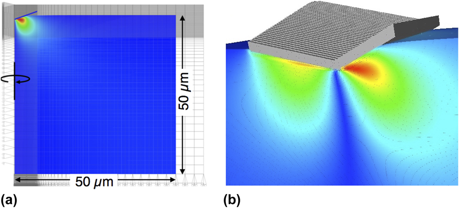
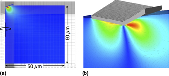
The geometry for 2D, axisymmetric simulationsReference Nairn and Guilkey29 of nanoindentation is shown in Fig. 1(a). In axisymmetric simulations, the indenter has a conical tip, which differs from most experiments that use a pyramidal Berkovich indenter. Axisymmetric simulations, however, allow much faster simulations and thereby more testing of simulation variables. Much nanoindentation analysis similarly relies on axisymmetry for tractability.Reference Oliver and Pharr30,Reference Clausner and Richter31 To maximize similarity between conical indenter and a Berkovich pyramid, the angle of the cone was chosen such that the projected contact area as a function of indentation depth is the same for both shapes. For a Berkovich indenter with a tip angle of 65.3°, the equivalent cone has a tip half-angle of θ = 70.3°.Reference Oliver and Pharr1,Reference Oliver and Pharr30
Axisymmetric MPM simulation of nanoindentation with colors (or shades of gray) showing radial displacement. (a) The full modeled specimen from an axisymmetric simulation. (b) Zoomed-in view of the absolute value of transverse displacements from a 3D simulation using a Berkovich indenter.

The axisymmetric block used for indentation was a rectangular block with symmetry conditions along the r = 0 plane, zero-velocity grid boundary conditions on the bottom, and free surfaces on the top and right edges. The indenter was modeled with rigid material points that were slanted to accurately represent the cone angle and the indenter surface. The goal of most simulations was to simulate nanoindentation on a large bulk object. To achieve this goal, the size of the block was varied until it no longer influenced the simulations. For a nanoindentation depth of 1.5 μm, which was chosen to reach indentation load of 5 mN for simulated materials, the block radius and depth had to be 0.05 mm or larger. Figure 1(a) shows radial displacements during an axisymmetric simulation of a sufficiently large block.
Although most simulations were axisymmetric, we also ran 3D simulations with a Berkovich indenter to verify similarity to axisymmetric simulations. The 3D simulations used a block of material ±0.05 mm in transverse directions and a depth of 0.05 mm. The simulations modeled half the block by cutting at its mid-plane and applying symmetry boundary conditions. The top and side surfaces were stress free; the bottom surface had zero-velocity boundary conditions. Figure 1(b) shows a zoomed-in view of absolute value of transverse displacements during a 3D simulation (absolute value was plotted for better comparison to axisymmetric results).
B. Material modeling
The indenter was modeled as a rigid material. All indenter particles were pushed into the material at a prescribed velocity. After reaching a desired maximum indentation load, the indenter particles reversed direction and returned to their initial positions at a prescribed reversing velocity. For simulations with strain-rate dependent yield properties, the indenter load was held constant for selected periods of time before reversing the particles. The rigid particle interacted with the bulk material by contact mechanics. A rigid indenter was used to allow simulations with larger time steps and to provide accurate, nondeforming contacting surfaces.
The material being indented was modeled as a neo-Hookean, hyperelastic–plastic material using J 2 plasticity with nonlinear and rate-dependent hardening laws. In the elastic region, this material uses the Mooney–RivlinReference Bower32 strain energy function with G 1 = G and G 2 = 0 or
 $$\matrix{ {W\left( {{\bf{F}},J} \right) = {G \over 2}\left( {{{{\rm{Tr}}\left( {{\bf{F}}{{\bf{F}}^T}} \right)} \over {{J^{2{\rm{/}}3}}}} - 3} \right)} { + {K \over 2}\left( {{1 \over 2}\left( {{J^2} - 1} \right) - \ln J} \right)\quad ,} \cr}$$
where  ${\bf{F}}$ is the deformation gradient,
 $J = \det \left( {\bf{F}} \right)$ is the relative volume change, and G = E/(2(1 + ν)), K = E/(3(1 − 2ν)), and E are the low-strain shear, bulk, and tensile moduli, respectively, and ν is the low-strain Poisson’s ratio. The Cauchy stress for this material is
 $$\sigma = {K \over 2}\left( {J - {1 \over J}} \right){\bf{I}} + {G \over {{J^{5{\rm{/}}3}}}}{\rm{dev}}\left( {{\bf{F}}{{\bf{F}}^T}} \right)\quad .$$
The nonlinear hardening law used in all simulations was
 $${\sigma _{\rm{y}}} = \left( {{\sigma _{{\rm{y}}0}} + {k_{\rm{h}}}{{\left\| {{{{\boldvarepsilon }}_{\rm{p}}}} \right\|}^{{n_{\rm{h}}}}}} \right)\left( {1 + C\ln \left( {{{\left\| {{{{{\dot{\boldvarepsilon }}}}_{\rm{p}}}} \right\|} \over {\dot{\varepsilon }_{\rm{p}}^{\rm{0}}}}} \right)} \right)\quad ,$$
where σy0 is the initial yield stress, k h and n h are hardening parameters, εp is the plastic strain, and C and  $\dot{\varepsilon }_{\rm{p}}^0$ describe strain-rate dependence of the yield stress. When C = 0, this law is rate-independent with power-law hardening. Nanoindentation experiments commonly hold at a constant maximum load before unloading. If modeled with a rate-independent material, this hold period would not be evident in the load–displacement curves. Experiments show, however, that indenter displacement increases while the load is held constant,Reference Chudoba and Richter33–Reference VanLandingham, Villarrubia, Guthrie and Meyers35 resulting in a flat spot on top of load–displacement curves. While this flat spot or “creep” could be thermal drift, most of it is material dependent and can be described by a logarithmic model.Reference Chudoba and Richter33 When C ≠ 0, the logarithmic term in Eq. (3) allowed us to investigate strain-rate effects. This term came from the Johnson–CookReference Johnson and Cook36 hardening law (the temperature-dependent term in the Johnson–Cook lawReference Johnson and Cook36 was omitted because all simulations were isothermal).
Contact between the rigid indenter and the plastic material was modeled using the contact methods described in Ref. Reference Nairn8. Because contact is crucial to nanoindentation simulations, the contact methods used here included a new option to improve detection of contact. Contact in MPM is modeled by extrapolating plastic material a and rigid material b to separate velocity fields on the grid.Reference Bardenhagen, Guilkey, Roessig, Brackbill, Witzel and Foster7,Reference Nairn8 Any node that “sees” both materials models contact mechanics in these simulations by the following three steps:
1. Find contact normal
The first step is to find a normal vector from material a to b using
 $${{{\hat{{\bi {n}}}}_i}\left\| {{{{{\hat{\bi n}}}}_i}} \right\| = \left\{ {\matrix{ { - {{\bi{g}}_{i,b}}} & {\left\| {{{\bi{g}}_{i,b}}} \right\| \ge {{\left\| {{{\bi{g}}_{i,a}}} \right\|} \over {100}}} \cr {{\Omega _{i,a}}{{\bi{g}}_{i,a}} - {\Omega _{I,b}}{{\bi{g}}_{i,b}}} & {{\rm{otherwise}}} \cr} } \right.\quad ,$$
where Ωi,j is the “domain” of material j and gi,j is the “domain” gradient of material j found by extrapolating domains of particles to node i on the grid using gradient shape functions.Reference Nairn8 For 3D simulations, the “domain” is the particle volume, but for axisymmetric simulations, the “domain” is the area of the material point in the r–z plane and not its volume.Reference Nairn8 The first option is using the rigid material volume gradient option in Ref. Reference Nairn8. The second option switches to the average volume gradient option in Ref. Reference Nairn8 for nodes in which the domain gradient of the rigid material is very small.Reference Lemiale, Hurmane and Nairn37 Axisymmetric simulations made use of symmetry to set normal vector for nodes along the r = 0 symmetry plane to be  ${{{\hat{\bi n}}}_i} = \left( {0,1} \right)$. Similarly, nodes on the 3D mid-plane of symmetry enforced normal vectors to have zero component perpendicular to that symmetry plane.
2. Detect contact
The second step is to determine if the two materials are in contact. A necessary condition is that the materials are approaching each other or that  $\left( {{{\bi{v}}_{i,b}} - {{\bi{v}}_{i,a}}} \right) \cdot {{{\hat{\bi n}}}_i} \lt 0$, but this condition is not sufficient. Contact detection is improved by also requiring that edges of material domains are in contact or that d i,b − d i,a ≤ 0, where d i,j is the distance along the normal vector from the edge of material j to node i.Reference Nairn8 The calculation of d i,j is done by extrapolating material point positions to the grid. For a material j, we can find an “apparent” distance from extrapolated particle position (xi,j as can be seen in Ref. Reference Nairn8) to node i (at xi) using
 $$d_{i,\,j}^{\left( {{\rm{ext}}} \right)} = \left( {{{\bi{x}}_{i,\,j}} - {{\bi{x}}_i}} \right) \cdot {{{\hat{\bi n}}}_i}\quad ,$$
but this distance will not equal the desired edge distance d i,j. An accurate use of edge positions in contact detection requires definition of a function  ${d_{i,j}}\left( {d_{i,j}^{\left( {{\rm{ext}}} \right)}} \right)$ to calculate actual edge distance from extrapolated “apparent” distance. Reference Reference Nairn8 proposed a simple constant correction that is equivalent to linear mapping functions:
 $${d_{i,j}}\left( {d_{i,j}^{\left( {{\rm{ext}}} \right)}} \right) = \left\{ {\matrix{ {d_{i,a}^{\left( {{\rm{ext}}} \right)} + 0.4\Delta x} & {j = a} \cr {d_{i,b}^{\left( {{\rm{ext}}} \right)} - 0.4\Delta x} & {j = b} \cr} } \right.\quad .$$
For these nanoindentation simulations, we instead implemented nonlinear mapping functions given by
 $${{{d_{i,j}}\left( {d_{i,j}^{\left( {{\rm{ext}}} \right)}} \right)} \over {\Delta x}} = \left\{ {\matrix{ {1 - 2{{\left( {{{ - d_{i,a}^{\left( {{\rm{ext}}} \right)}} \over {1.25\Delta x}}} \right)}^{0.58}}} & {j = a} \cr { - 1 + 2{{\left( {{{d_{i,b}^{\left( {{\rm{ext}}} \right)}} \over {1.25\Delta x}}} \right)}^{0.58}}} & {j = b} \cr} } \right.\quad .$$
These functions were determined by explicit calculations of  $d_{i,j}^{\left( {{\rm{ext}}} \right)}$ as a function of d i,j for either convected particle domain integration shape functions (CPDI introduced in Ref. Reference Sadeghirad, Brannon and Burghardt38) or undeformed generalized interpolation material point shape functions (uGIMP, introduced in Ref. Reference Bardenhagen and Kober10), inverting the results, and fitting to a power law. The calculation process and plots of calculations are given in the Supplementary Material.
3. Add contact forces
For any multimaterial node detected to be in contact, the last step in rigid material contact is to apply contact force to material a by changing its extrapolated momentum. For contact with rigid materials, this task first finds momentum change required for material a to “stick” to the rigid material as Δpi,a = m i,a(vi,b − vi,a), where m i,a is the extrapolated mass of material a. This momentum change implies normal and tangential contact forces to “stick” to the rigid material of
 $${{\bi{f}}_{\rm{n}}} = {{\left( {\Delta {{\bi{p}}_{i,a}} \cdot {{{{\hat{\bi n}}}}_i}} \right)} \over {\Delta t}}{{{\hat{\bi n}}}_i}\quad {\rm{and}}\quad {{\bi{f}}_{\rm{t}}} = {{\left( {\Delta {{\bi{p}}_{i,a}} \cdot {{{{\hat{\bi t}}}}_i}} \right)} \over {\Delta t}}{{{\hat{\bi t}}}_i}\quad ,$$
where Δt is the time step and  ${{{\hat{\bi t}}}_i}$ is the unit vector in the tangential direction of motion. These simulations used contact with Coulomb friction. For this contact law, the final momentum change applied to material a is
 $$\Delta {\bi{p}}_{i,a}^\prime = \left\{ {\matrix{ {\Delta {{\bi{p}}_{i,a}}} \hfill & {{f_{\rm{t}}} \lt - \mu {f_{\rm{n}}}} \hfill \cr {\left( {\Delta {{\bi{p}}_{i,a}} \cdot \widehat {{{\bi{n}}_i}}} \right)\left( {\widehat {{{\bi{n}}_i}} - \mu \widehat {{{\bi{t}}_i}}} \right)} \hfill & {{\rm{otherwise}}} \hfill \cr} } \right.\quad ,$$
where μ is the coefficient of friction.Reference Bardenhagen, Guilkey, Roessig, Brackbill, Witzel and Foster7,Reference Nairn8 The first form is “stick” conditions while the second is for frictional “slip.” The final change in momentum implies a contact force on node i of 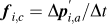 ${{\bi{f}}_{i,c}} = {{\Delta {\bi{p}}_{i,a}^\prime } / {\Delta t}}$. We summed all nodal contact forces to track the indenter load on the nonrigid material.
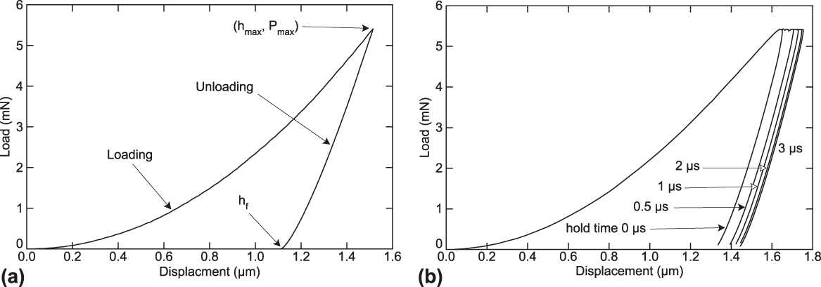
All simulations used explicit MPM methods, which means the time step must follow Δt < Δx/w, where w is the wave speed of the material. For modeling to be possible in a reasonable time frame, we used loading rates much higher than in typical experiments and relied on two techniques to mitigate or eliminate dynamic effects. First, the prescribed indenter velocity was chosen such that indenter displacement as a function of time was sigmoidal in both the loading and unloading phases. This approach helped reduce stress waves induced by impulses associated with constant-velocity loading and its abrupt shift to constant-velocity unloading. Second, we used a new MPM velocity update scheme called XPIC(2).Reference Hammerquist and Nairn39 This update scheme suppresses noise and high frequency velocity waves not appropriate in quasi-static simulations without causing over-damping. Figure 2(a) gives a typical simulated load–displacement curve by cross-plotting simulated load and applied sigmoidal displacement. The sigmoidal speed varied from 0 to 1.3 m/s, which for the simulated materials was less than 0.1% of its wave speed. Loading faster introduced dynamic effects while loading slower gave identical results. We thus used the maximum possible speed such that sigmoidal loading and XPIC(2) updates were sufficient to provide results equivalent to noise-free, quasi-static loading.
(a) Cross plot of load output versus displacement input for typical simulated indenter load as a function of displacement for both loading and unloading. (b) Simulated load–displacement curves for a strain-rate dependent material with C jc = 0.1 for different hold times.

C. MPM grid
Simulation output provides a virtual nanoindentation experiment for indenter load (from contact forces) versus displacement (from position of rigid indenter particles). We varied cell sizes to determine necessary spatial resolution for convergence. We found, not surprisingly, that necessary grid cell size scales with depth of indentation, i.e., deeper indentation can use lower resolution. For the range of depths studied, we found that 100-nm cells, which correspond to 50-nm particles when using two particles per cell in each dimension, gave converged results.
Most MPM modeling uses a regular grid of equally sized cells. Regular grids are used because of simplicity afforded to some calculations and because they are needed in problems with large movement through the grid.Reference Stomakhin, Schroeder, Chai, Teran and Selle19,Reference Wang, Beom, Sun and Lin21,Reference Nairn26,Reference Mast, Arduino, Miller and Mackenzie-Helnwein40 The literature on mesh refinement in MPM is sparse. A few examples can be found in Refs. Reference Hu, Xue, Mao, Kamakoti, Zhao, Dittakavi, Wang, Li, Ni and Brenner27, Reference Mao, Chen, Li and Feng41, and Reference Ma42. The nanoindentation problem modeled here is an excellent candidate for mesh refinement. We know that throughout the simulation, we need a refined mesh only under the indenter tip. All regions remote from the indenter can be modeled with sufficient accuracy by using larger grid cells and material points.
For nanoindentation simulations, we used a grid scheme termed a “tartan” grid. In a tartan grid, one or more “regions of interest” are modeled with a high-resolution, regular grid with equally sized elements. For the nanoindentation problem, the one region of interest under the indenter was modeled with 100-nm cells determined above as needed for convergence. Outside regions of interest, the grid cell sizes were allowed to increase, thus forming a tartan-like pattern.
A tartan grid maintains orthogonal grid lines, which greatly simplifies its implementation compared to arbitrary background grid cell sizes. The changes needed for a tartan grid depend on the MPM shape functions being used and are easily implemented for CPDI shape functions.Reference Sadeghirad, Brannon and Burghardt38 In brief, CPDI shape functions for both Cartesian gridsReference Sadeghirad, Brannon and Burghardt38 and axisymmetric gridsReference Nairn and Guilkey29 depend only on current size of the particle and element shape functions evaluated at the corners of the current particle domain. Thus any current CPDI code automatically supports a tartan grid provided the shape function calculations recognize variable particle sizes and variable element sizes when finding the shape functions at the corners. Classic MPM shape functionsReference Sulsky, Chen and Schreyer11 similarly support tartan grids with little modification, but such shape functions are never recommended for accurate simulations. The changes required for uGIMP shape functions are more substantial. Implementation of uGIMP shape functions is typically done by analytical solution to the GIMP integral as a function of particle position in a cell and that integral may involve integration over neighboring cells.Reference Bardenhagen and Kober10 For a regular grid, the analytical functions are the same for all particles. Implementation of a tartan grid would not be difficult but would require re-evaluation of all integrals allowing for variable size particles and variations in sizes of cells surrounding each node.
All simulations here used tartan grid and CPDI shape functions. The grid spacing outside the region of interest was increased with a linear ratio: Δx t = nRΔx, where n is the number of cells away from the region of interest, R = 2 is the size ratio, and Δx = 100 nm is the cell size in the region of interest. For 2D, axisymmetric simulations, we verified that tartan grid results gave virtually identical results as a regular grid with equal-sized cells. By using a tartan grid, however, we could reduce the number of particles by an order of magnitude, which also reduced simulation time by an order of magnitude. Full 3D simulations using our resources (Dell servers with 32, 3 GHz, Xeon processors) and tartan grids took 10+ h. 3D grids without tartan grids in a reasonable time would require significantly more processors. The Supplementary Material illustrates the tartan grids used along with some additional details.
Besides shape function calculations, tartan grids also require modification of any contact calculations that depend on grid size.Reference Nairn, Bardenhagen and Smith9 For example, the calculation of material separation described above depends on cell length or Δx. For regular grid with square (2D) or cubic (3D) cells, grid dimensions are the same in all directions and Δx is the appropriate factor. For a regular grid with equally sized rectangular (2D) or rectangular cuboid (3D) cells, Δx needs to change to h ⊥ which is an effective cell-size normal to the contacting plane.Reference Nairn8 For a tartan grid, Δx (and some other contact calculations) must be changed further to account for sizes of all cells surrounding node i. For these nanoindentation simulations, all contacting nodes were located in the region of interest that had equally sized elements. The contact calculation methods explained above for a regular mesh could therefore be used without modification. The changes for general contact in a tartan grid will be in a future publication.
III. RESULTS AND DISCUSSION
Nanoindentation simulations described above predict the load–displacement curve for nanoindentation experiments on any material with known constitutive law in any specimen with known geometry [typical curve in Fig. 2(a)]. The constitutive law used here was for neo-Hookean, hyperelastic–plastic materials, but the simulation method could be used with other material models such as models including thermal effects, rate-dependence, and brittle failure processes. If the material and indenter have comparable properties, the simulations could explicitly model the indenter rather than assume a rigid indenter. One application of such simulations would be to vary material properties until simulations and experiments agree. Although this use of simulations has potential future uses (especially for nanoindentation on materials with complex morphology such as wood cell wallsReference Jakes, Frihart, Beecher, Moon and Stone34), another application of simulations is to validate conventional methods for interpreting nanoindentation experiments. In brief, these simulations can be treated as accurate and low-noise virtual experiments on a material with precisely known properties and on various geometries of the indented object. In this section, we subject such virtual experiments to various analysis methods to see if those methods correctly extract the input material properties.
A. Analysis of load–displacement curves
The Oliver–Pharr method to interpret nanoindentation experiments is based on nanoindentation of an isotropic material in an infinite half-space. We can apply their methods to results from simulations on an isotropic bulk with length and width large enough to represent an infinite half-space. In the Oliver–Pharr method, the unloading portion of the curve is modeled with a power law:
 $$P\left( h \right) = \alpha {\left( {h - {h_{\rm{f}}}} \right)^m}\quad ,$$
where P is the contact force, h is the indenter depth, h f is the final depth (i.e., the depth at which the load returns to zero), and α and m are fitting parameters. The measured modulus of the material is deduced from the initial slope of the unloading curve at h = h max [denoted as S = dP(h max)/dh = αm(h max − h f)m−1] and the maximum projected area of contact, A c, between the indenter and the material using
 $${E \over {1 - {\nu ^2}}} = {1 \over \beta }{{\sqrt \pi } \over 2}{S \over {\sqrt {{A_{\rm{c}}}} }}\quad ,$$
where β is an empirical parameter used to account for all physical processes that might affect S (e.g., indenter shape or properties of the indented material).Reference Oliver and Pharr30 The β parameter was chosen in early work to be unity but is now recognized as larger. Oliver and PharrReference Oliver and Pharr30 recommend β = 1.05 as good choice for a range of materials. The material’s hardness can also be determined from the maximum load and contact area:
 $$H = {{{P_{\max }}} \over {{A_{\rm{c}}}}}\quad .$$
Calculation of E or H relies on measurement of A c. For the axisymmetric cone used here, a geometric calculation of projected contact area gives
 $${A_{\rm{c}}}\left( h \right) = \pi {h^2}{\tan ^2}\left( {{{70.3}^\circ }} \right)\quad ,$$
(note: cone angle 70.3° was chosen to give identical A(h) function as Berkovich indenter with angle 65.3°). Unfortunately, one cannot use h max in this equation because the measured displacement combines both penetration into the material and “sink-in” deflection of the surface away from the indenter.Reference Oliver and Pharr30 The standard analysis method accounts for “sink-in” by correcting h max to give an actual contact depth, h c, using
 $${h_{\rm{c}}} = {h_{\max }} - \varepsilon {{{P_{\max }}} \over S} = {{\left( {m - \varepsilon } \right){h_{\max }} + \varepsilon {h_{\rm{f}}}} \over m}\quad ,$$
and then finding contract area from A c(h c).Reference Oliver and Pharr30 The parameter ε depends on material properties and geometry of the indented material. Calculations for an isotropic, elastic material in an infinite half-space show that ε depends on m from the unloading curve and varies from 0.74 to 0.79 for typical values. For simplicity, it was suggested that ε = 0.75 provides a good overall value, although a function to find ε from m for isotropic, elastic, infinite, half-space is an available option.Reference Oliver and Pharr30
Our baseline simulation used E = 2.0 GPa, ν = 0.3, ρ = 1.2 g/cm3, σy0 = 30 MPa, k h = 100 MPa, n h = 0.5, and C = 0. We first interpreted the virtual load–displacement curves using the Oliver–Pharr simplification that β = 1.05, but different options for finding ε. References Reference Oliver and Pharr1 and Reference Larsson, Giannakopoulos, Söderlund, Rowcliffe and Vestergaard43 suggest that power-law fits to only the top 33% (or even top 10%) of unloading curves are sufficient for determining unloading parameters. To test this suggestion, the power law in Eq. (10) was fit to various fractions of the unloading curves using R.44 Initial parameters were obtained by fitting a linear model to the log-transformed data. These parameter estimates were then refined to fit the curves by nonlinear least squares using R’s built-in function optim(). All power-law fits to our simulated curves were essentially perfect with R 2 values always greater than 0.99999. Nevertheless, due to nature of power laws, the fitting parameters depended on fraction fit—m varied from 1.05 to 1.32; α varied from 33.5 × 10³ to 1460 × 103 N/mm; h f varied from 1.08 to 1.16 μm.
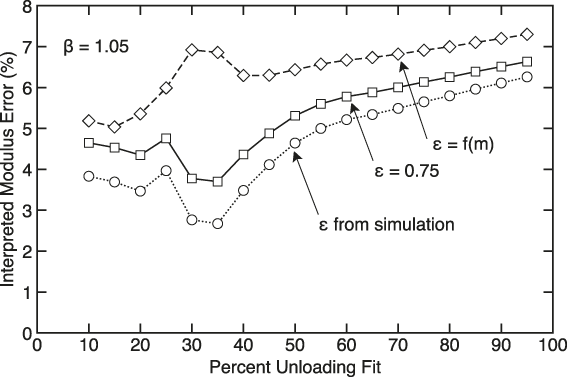
Figure 3 plots percent error in effective modulus (E eff = E/(1 − ν2) compared to input E eff = 2.198 GPa) extracted from simulated curves by three different methods for finding ε. First, notice that results vary widely when fraction fit is less than 60%. Because this region is fitting a narrow range in h, the power-law results are not reliable. The results for 60% and higher are reliable and consistent; the variations below 60% are not meaningful. The solid curve (square symbols) assumed ε = 0.75. The extracted modulus for 60% or more fit is about 5% too high and the error increased slightly as more of the unloading curve was fit. The dashed line (diamond symbols) found ε from relation in Ref. Reference Oliver and Pharr30. For the range of m seen in these data, the calculated ε ranged from 0.77 to 0.86, but increasing ε caused larger errors compared to actual modulus.
The percent error in effective modulus extrapolated from simulated nanoindentation curves as a function of the percentage of the unloading curves used in the analysis. The three curves are for three methods for choosing ε in the analysis method. All curves used β = 1.05.

Rather then find ε from a relation that was derived for an elastic material,Reference Oliver and Pharr30 the last method was to “measure” A c from simulation output; i.e., find ε for an plastic material by numerical methods. All particles in contact with the indenter were in compression (in the depth direction), while the first surface particle at the edge of contact was in tension. The radial position of this tensile particle equals the radius of the projected contact area or h c tan θ (±25 nm or half a particle size). From this simulated h c and fits to unloading curves, the simulation results corresponded to ε ranging from 0.711 to 0.736 or always lower than 0.75. Using these numerically determined ε′s, the extracted modulus is slightly closer to the correct result.
This baseline simulation analysis suggests that modulus calculation should analyze at least 60% of the unloading curve and ε is best found from measured h c. Because measuring h c may not be possible, a value of ε = 0.75 is as good, or preferable to, finding ε from the relation for an elastic material in Ref. Reference Oliver and Pharr30. An observation that fitting less than 60% of an experimental unloading curve, R 2 > 0.99 still does not support a claim that fitting parameters are reliable.
Even when ε is numerically determined from known material properties (i.e., using simulation results), the extracted modulus is still 5% or more higher than actual modulus of the material. This discrepancy can be interpreted as the use of an incorrect value for the β parameter. In other words, by changing β, the extracted E eff can be made to exactly match the input value. Using the reasonable ε = 0.75, the results when using 60% or more of the unloading curve give exact results if β is varied from 1.111 to 1.118. This higher β is consistent with prior calculations. Larsson et al.Reference Larsson, Giannakopoulos, Söderlund, Rowcliffe and Vestergaard43 conducted finite element experiments for linear elastic materials and found β dependent on ν with β = 1.14 at ν = 0.3. Oliver and PharrReference Oliver and Pharr30 mentioned that β is higher for materials with strain hardening. References Reference Jakes, Frihart, Beecher, Moon and Stone34 and Reference Troyon and Lafaye45 also claimed that β should be higher and closer to 1.09. Our simulations, which are consistent with these previous findings, show that the β depends on both elastic and hardening properties of the material. When performing nanoindentation on an unknown material, the correct value of β will not be known. Choice of values between 1.05 and 1.14 will therefore have uncertainties in the range of ±5%.
B. Hardening parameters
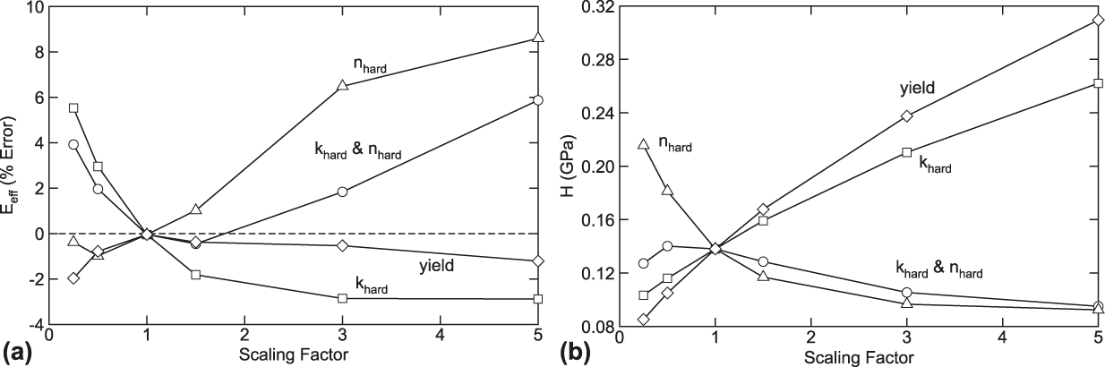
This section explores the effect of changing material plasticity properties on the modulus and hardness extracted with the Oliver–Pharr method. The baseline properties were from Sec.III.A. These additional simulations varied yield stress, σy0, hardening modulus, k h, and hardening exponent, n h, about the baseline values. Four sets were run: vary only k h, vary only n h, vary k h and n h together, and vary only σy0. For each set, the variable parameter was scaled by factors 0.25, 0.5, 1.5, 3, and 5 relative to the baseline value while all other parameters were held at their baseline value. Based on the results in Sec.III.A, the effective moduli and hardness were extracted by analyzing 75% of the unloading curve and using ε = 0.75 and β = 1.115.
The percent error in the calculated effective moduli for these simulations as a function of scaling factor is shown in Fig. 4(a). The yield stress had the smallest effect while strain hardening parameters had larger effects. When k h and n h were varied together, the results increased almost as much as varying n h alone suggesting that n h is the dominate hardening parameter affecting the analysis.
Effect of scaling the hardening parameters on parameters extracted from load–displacement curves. (a) Percent error in calculated effective modulus. (b) Calculated hardness. All curves used ε = 0.75 and β = 1.115.

The errors in measured effective moduli varied from −2.9 to 8.6%. Because these errors occurred by varying material properties other than modulus, we suggest that the Oliver–Pharr method should never expect better than about ±10% accuracy for a material with unknown hardening properties. Improving accuracy of nanoindentation experiments would require analysis methods that can account for both a material’s stiffness and its hardening properties. One option would be to use inverse methods and vary all material properties until the full, simulated load–displacement curve matches experimental results. Because this process would use the full curve, it has more potential to detect effects of material hardening (the loading portion of the curve depends on hardening parameters more then the unloading portion). This approach was used with some success for analysis of nanoindentation experiments on materials with gradient properties.Reference Nardi, Hammerquist, Nairn, Karimi, Månson and Leterrier5 Their inverse methods could find E eff, K, and n by inverse methods. They found that the results were insensitive to σy0, which is consistent with above observation that varying σy0 had the smallest effect on the unloading curve. The simulations in Ref. Reference Nardi, Hammerquist, Nairn, Karimi, Månson and Leterrier5 were lower resolution and had more noise. The simulations here with tartan grid and methods for reducing noise should lead to improved inverse analysis of nanoindentation experiments.
The calculated hardness H for these simulations relative to baseline values and as a function of scaling factor is shown in Fig. 4(b). Unlike modulus, the H value for any material is not an input to simulations and therefore extracted H cannot be compared to a known value. Experiments for hardening are mostly qualitative and express some number based on final indent size relative to indentation pressure. A simulated material’s hardness should therefore vary with change in hardening properties and results in Fig. 4(b) track expectations. The measured H increases as σy0 or k h increases. The variation with n h is also expected. For power-law hardening with constant σy0 and k h, hardening curves for various n h intersect when ‖εp‖ = 1 (or 100% plastic strain). Because all simulations show that ‖εp‖ remained less than 1 for all material points (except sometimes a few points directly under the indenter tip), increasing n h will shift the hardening curve closer to an elastic–plastic material with lower hardness. Conversely, decreasing n h will shift the curve to a material with higher yield stress and higher hardness. The dependence of H on n h follows this expected trend. The curve that varied k h and n h again shows that n h is the dominant hardening parameter affecting indentation experiments.
C. Strain-rate dependent materials
The goal of simulations with time-dependent strain hardening [i.e., when C ≠ 0 in Eq. (3)] was to mimic typical experiments where indenter load is held constant for some time period before unloading. Because load is held constant, we had to switch from indenter velocity control to load control simulations. The rigid particles used in these simulations were constant-velocity particles that effectively have infinite mass. Because applying loads to infinite-mass particles would not affect their velocity, we implemented a PID (Proportional, Integral, Derivative, controller, see Ref. Reference Graf46) feedback loop to control indenter velocity. This loop compared a target force function to the current contact force, which was determined by summing all contact forces on the rigid indenter. The feedback control modified indenter velocity to achieve the desired force function. As in velocity control simulations, the PID loop was based on a target load as a function of time that was sigmoidal both in the loading and unloading phase to prevent oscillations. To simulate experimental procedures, the target load function had a hold phase at constant maximum load for variable amounts of time.
These simulations used the same baseline properties as above, but now varied C from 0.01 to 0.1. The reference strain-rate parameter, or strain rate at which hardening is equal to baseline hardening, was set to  $\dot{\varepsilon }_{\rm{p}}^0 = {10^6}\;{{\rm{s}}^{ - 1}}$. This reference rate was set to 1/(loading time) for the simulations, where loading time was 1 μs. Because the loading rate (or maximum displacement over loading time of about 1 m/s) was much less than 1% of the material’s wave speed, these simulations can be considered as quasi-static results where the only rate effects would be rate-depending yielding of the material. In other words, although the simulations were much faster than experiments, the time axis can be viewed as reduced time relative to the reference strain-rate parameter. Predictions at slow rates with real materials could be made by rescaling the time axis to any new reference strain rate. For positive C, particles loaded below the reference rate will see drop in yield stress while those at higher rates will see higher yield stress. Figure 2(b) gives simulated nanoindentation curves with C = 0.1 and various hold times at maximum load. The PID load control worked well, giving simulations that were relatively free from noise and that contained a stable hold phase at constant maximum load. The quasi-static character of these simulations is confirmed by small oscillations in the plateau region (and some of the oscillations may be caused by PID control parameters).
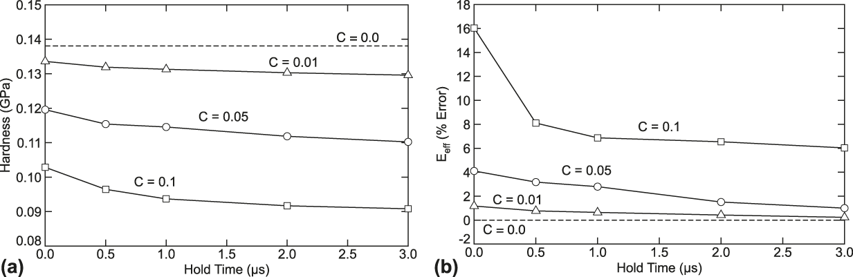
We looked at the effect of hold time for a strain-rate dependent yield material on both the hardness and the effective modulus extracted from simulated results by the Oliver–Pharr method (and assuming ε = 0.75 and β = 1.115). Figure 5(a) shows measured hardness compared to baseline hardness (horizontal line for C = 0). Increasing C caused the hardness to drop and the drop increased with C. The drop in hardness occurred because plastic strain rates under the indenter were always less than the chosen reference strain rate. As a result, the strain-rate term causes a drop in yield stress or a material with lower hardness. As a function of time, the hardness dropped further. During the hold phase the plastic strain rate is very low leading to further drop in yield stress.
Effect of C jc and hold times on parameters extracted from load–displacement curves. (a) Calculated hardness. (b) Percent error in calculated effective modulus. All curves used ε = 0.75 and β = 1.115.

Figure 5(b) shows the effects of C and hold time on percent error in the extracted effective modulus. E eff error increased with zero hold time and the increase was larger for higher C. The increase was caused by change in strain hardening properties of the material. As can be seen in Fig. 4(a), the change in E eff with changes in hardening-law properties are more convoluted than changes in hardness. For all values of C, the extracted E eff decreased with time and perhaps reached a plateau. As a consequence, experiments on materials with strain-rate dependent hardening properties should use sufficient hold time to reach plateau, or at least consistent, results for both hardness and modulus.
D. Shape effects
Many methods for extracting E eff from experiments and analyzing effects of material hardness are based on indentation of a homogeneous infinite half-space, or a good approximation of such a space. If this assumption is significantly violated, the standard nanoindentation analysis methods cannot be trusted. Reference Reference Jakes, Frihart, Beecher, Moon and Stone34 presents an experimental method to correct for shape effects. They propose modeling total compliance C t of the indentation system using
 $${C_{\rm{t}}} = {1 \over {{E_{{\rm{eff}}}}\sqrt {{A_{\rm{c}}}} }} + {C_{\rm{m}}} + {C_{\rm{s}}}\quad ,$$
where C m is the compliance of the machine and C s is any additional compliance of the indentation specimen due to deviation from being a homogeneous, infinite half-space. The term  ${E_{{\rm{eff}}}}\sqrt {{A_{\rm{c}}}}$ is proportional to slope S in Eq. (11). The machine compliance should be fairly constant (and zero for simulations), but the structural compliance could vary significantly with location of the indentation on a specimen. For example, indentation on one material near an interface with another material or indention near a free edge would both see C s change as a function of distance to the interface or the edge. In principle, by running experiments as a function of indentation location, one could measure C s allowing one to separate material E eff from machine and specimen compliance effects. Reference Reference Jakes, Frihart, Beecher, Moon and Stone34 proposes that the effect of some structural demarcation should be a function of the inverse of its distance to the nanoindentation site.
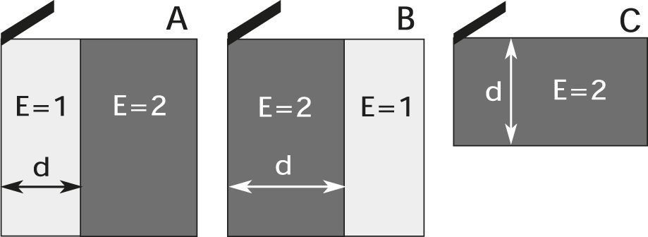
To investigate the strategy from Ref. Reference Jakes, Frihart, Beecher, Moon and Stone34, we conducted three numerical experiments using MPM simulations as illustrated in Fig. 6. First, the indentation block was divided into two materials with the material under the indenter have E = 1.0 GPa while the remainder of the block had E = 2.0 GPa. The variable d was the distance from the indenter tip to the material interface. Second, the two materials were switched such that the stiffer material was under the indenter. Third, the entire block had E = 2.0 GPa but the depth of the block was varied—d was now the distance from the indenter tip to the rigid, zero-velocity surface on the bottom of the block. The plasticity properties used the baseline properties from Sec. III.A.
Axisymmetric simulation geometries used to investigate the effect of structure on shape. d is the distance from indentation tip to a key structural change. A—Low stiffness material surrounded by high stiffness material (moduli in GPa). B—High stiffness material surrounded by low stiffness. C—Thin material.

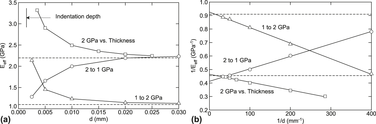
The calculated E eff from simulated load–displacement curves for the three different structural geometries are plotted in Fig. 7(a). Not surprisingly, E eff varies significantly when d is small or when the indented specimen has significant deviations from a homogeneous, infinite half-space. Also note that the effect persists to a rather large d. The measured E eff did not return to input material properties until d was more than 20 times the indentation depth, which was 1.5 μm [see Fig. 7(a)]. It would be a misconception to think that because nanoindentation tips and depths are small that the method is not altered by even relatively remote structural features.
The effect of distance to a structural change on effective modulus extracted from simulated nanoindentation curves. The horizontal dashed lines are the actual effective moduli. Plots a and b show the same date plotted in two different ways.

Reference Reference Jakes, Frihart, Beecher, Moon and Stone34 discusses two ways to correct for structural compliance in nanoindentation experiments. One method requires measurement of the contact area from the indentations while the second requires multiple indentations in the same area with different maximum loads. Here we used a third method that was made possible because we know the correct modulus. We assumed that the structural effects should be described by some function of d, which can be formulated as
 $${1 \over {{E_{\rm{m}}}\left( d \right)}} = {1 \over {{E_{{\rm{eff}}}}}} + f\left( d \right)\quad ,$$
where E m(d) is the measured modulus from simulation of the material with known E eff and f(d) is some nonconstant function. By examining simulation results, f(d) appears well represented by a linear function of 1/d. In other words, plots of 1/E m(d) as a function of 1/d are close to linear with the intercept being close to 1/E eff [see Fig. 7(b)]. Extrapolating to d → ∞ (or 1/d → 0) gives an estimate for E eff with an error of 10% for the geometry A (“1–2 GPa”) in Fig. 6, 2% for geometry B (“2–1 GPa”) and 2% for geometry C (“2 GPa versus thickness”). The larger error for geometry A was likely because the material under the indenter had E = 1.0 GPa while the data was interpreted using β determined in Sec. III.A for a material with E = 2.0 GPa.
E. Full 3D simulation and effective indenter shapes
We repeated the baseline simulations in Sec. III.A using a full 3D model with a pyramidal Berkovich indenter. A simulation of the same size block extended to 3D using a tartan grid and using slightly lower resolution under the indenter (150-nm cells) needed about nine million particles and ran in about two days. A simulation with 100-nm cells under the indenter is feasible but required about 30 million particles and would take several weeks. The results at 150 nm resolution looked acceptable. As can be seen in Fig. 1, the transverse displacement under the indenter in 3D resembles the corresponding radial displacement in axisymmetric simulations. The 3D simulation does reveal asymmetry in the displacement caused by asymmetry in the Berkovich indenter shape along the symmetry plane. Despite asymmetry effects in the 3D stress state, the global load–displacement curves for the full 3D simulations were almost identical to curves from axisymmetric simulations. Compared to axisymmetric simulations, the 3D simulation had about 3% higher peak load, had the same hardness, and had about 7% higher extracted E eff. The small differences persist even if compared to axisymmetric simulations with 150-nm cells, which means they are likely caused by indenter shape effects. The overall similarities between axisymmetric and 3D results are reassuring as much nanoindentation analysis is carried out using axisymmetric methods.Reference Oliver and Pharr1–Reference Poon, Rittel and Ravichandran3,Reference Oliver and Pharr30
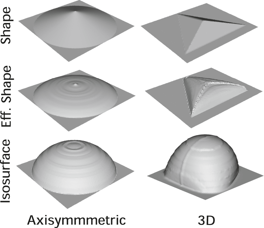
While a Berkovich indenter is not conical, its agreement with conical simulations can be partially explained by the concept of an effective indenter discussed in Ref. Reference Pharr and Bolshakov47. When an indenter is being pressed into a surface, any plastic deformation will blunt or smooth the indenter shape seen by the purely elastic portion of the material. During the unloading, the deformed region and the indenter form a blunted “effective indenter” under which the pressure is approximately constant. For the power law in Eq. (10) describing the unloading portion of the curve, an elastic material should have m = 1 for a flat punch and m = 2 for a cone or Berkovich indenter. In nanoindentation experiments (and simulations), this parameter is generally between these two. In our axisymmetric simulations, we found m ≈ 1.25 (provided at least 60% of unloading curve was fit), which is consistent with the concept of an effective indenter. Reference Reference Pharr and Bolshakov47 suggests that the effective indenter shape can be found by measuring the difference between the final indentation shape and the indenter. Because simulations give full details for indentation shape, this proposed effective indenter shape can be calculated. The effective shapes for both our axisymmetric and 3D simulations are visualized in Fig. 8. These shapes are fairly blunt for both cases, which is consistent with m decreasing toward value for a flat punch and partially explains similarities of the results.
Comparison of the actual indenter shapes, effective indenter shapes, and an isosurface of vertical compressive stress of 30 MPa under the indenter. The vertical axis for the shapes was made five times larger and all the geometries are flipped upside down, and the flat surface was added for better viewing perspective.

For another view, we looked at an isosurface of constant compression stress of 30 MPa in the depth direction. These isosurfaces do not correspond well to the shape of the effective indenters, as would be expected from a uniform pressure under an indenter. As pointed out in Ref. Reference Fu and Cao48, it is not actually possible to have uniform pressure under an indenter of any shape. Despite the lack of axisymmetry of the Berkovich indenter, the stress isosurface shown in Fig. 8 looks similar to the axisymmetric case, which illustrates again that indenter shape effects are blunted by plasticity and by dispersion of the stress distribution. Both effective indenter shapes and stress isosurfaces help explain why axisymmetric simulations are good approximations to 3D simulations with a pyramidal Berkovich indenter.
IV. CONCLUSIONS
These new simulations have demonstrated that MPM is well equipped for the modeling of nanoindentation. In particular, MPM handles well the large deformation and contact that occurs under the indenter tip. For good simulation results, the region under the indenter tip requires high resolution and that need was met efficiently by using a tartan grid. To achieve noise-free curves with no dynamic artifacts, the indenter displacement should be sigmoidal and the MPM calculations should use noise reduction methods now available in XPIC(m).Reference Hammerquist and Nairn39
All virtual experiments show that stiffness and hardness extracted from load–displacement curves depend on the hardening parameters of the material. If the hardening parameters depend on strain rate, the extracted stiffness and hardness will also depend on hold time at maximum load. Because one typically does not know the hardening parameters of a material studied by nanoindentation, these numerical observations suggest a limit on the accuracy achievable by using Oliver–Pharr methods. A potential approach to achieving higher accuracy is by using numerical analysis. For example, an iterative inverse approach coupled with MPM, as performed in Ref. Reference Nardi, Hammerquist, Nairn, Karimi, Månson and Leterrier5, could be used to solve for material parameters by matching load–displacement curves to experiments. If that analysis considers the full curve (i.e., both loading and unloading), such an inverse approach may find both stiffness and hardening properties of an unknown material. A note of caution—the load–displacement curves are a convolution of elasticity, plasticity, and local geometry and have been shown to not necessarily be unique.Reference Chen, Ogasawara, Zhao and Chiba49 Furthermore, if the material being indented is strain-rate dependent, resulting in the load displacement curves with a flat top, then this strain-rate dependence needs to be modeled as well. MPM could be an effective tool for carrying out inverse methods aimed at extracting additional and more-accurate material properties from nanoindentation experiments.
Supplementary Material
To view supplementary material for this article, please visit https://doi.org/10.1557/jmr.2018.75.
ACKNOWLEDGMENT
The work was funded by the National Institute of Food and Agriculture (NIFA) of the United States Department of Agriculture (USDA), Grant No. 2013-34638-21483.