





Introduction
Landscapes evolve due to tectonic and climatic forcing, ideally moving towards dynamic equilibrium (Gilbert, Reference Gilbert1909; Hack, Reference Hack1960), specifically balancing uplift with denudation (Whipple, Reference Whipple2004), leaving behind a complex record (i.e., topography; Dortch et al., Reference Dortch, Owen, Schoenbohm and Caffee2011; Dietsch et al., Reference Dietsch, Dortch, Reynhout, Owen and Caffee2015). Landslides play a significant role in transient topographic cyclicity over Quaternary time scales where successive changes in base level can drive vertical incision, both glacial and fluvial. The effect of landslides on regional- and catchment-scale denudation and landscape evolution is significant (DiBiase et al., Reference DiBiase, Whipple, Heimsath and Ouimet2010; Campforts et al., Reference Campforts, Shobe, Overeem and Tucker2022), although sometimes difficult to quantify (Dortch et al., Reference Dortch, Owen, Haneberg, Caffee, Dietsch and Kamp2009), as landslides communicate fluvial incision to ridges through hillslope adjustment (Willett, Reference Willett2010). Landslide activity is variable in frequency and magnitude across time and space and dependent on several geomorphic factors, such as hypsometry (Aristizábal and Korup, Reference Aristizábal and Korup2025), incision (Campforts et al., Reference Campforts, Shobe, Steer, Vanmaercke, Lague and Braun2020), and sediment accumulation (Parker et al., Reference Parker, Hales, Mudd, Grieve and Constantine2016). Erosion rates inferred from landslide frequency–size distributions have been recorded at the level of, or greater than, those of the tectonic uplift rate (Malamud et al., Reference Malamud, Turcotte, Guzzetti and Reichenbach2004; Larsen and Montgomery, Reference Larsen and Montgomery2012; Booth et al., Reference Booth, Roering and Rempel2013). These processes can be interlinked; rejuvenated landscapes are typically associated with a relative increase in landsliding and the presence of many landslides in the catchments of the southern Appalachians led to identifying regional uplift in the Miocene (Gallen et al., Reference Gallen, Wegmann and Bohnenstieh2013).
Landslides are an integral part of landscape evolution modeling, however, they are also a threat to humans and their built environments (Broeckx et al., Reference Broeckx, Rossi, Lijnen, Campforts, Poesen and Vanmaercke2020). The threat of landsliding turns modeling foci towards applied modeling of landslide susceptibility. Susceptibility models have the goal of modeling probability of occurrence of landslides over a landscape (Reichenbach et al., Reference Reichenbach, Rossi, Malamud, Mihir and Guzzetti2018), often employing some statistical method and an input dataset for training (i.e., data-driven approaches). Data-driven machine learning (ML) modeling of landslide susceptibility has a wide variety of parameterization options. These include the selection of modeling algorithm, hyperparameters, features (e.g., choosing slope angle or curvature as conditioning factors), and specifics of the training data (Reichenbach et al., Reference Reichenbach, Rossi, Malamud, Mihir and Guzzetti2018). ML applications for landslide susceptibility models are commonplace, and research continues to grow (Lima et al., Reference Lima, Steger, Glade and Murillo-García2022; Liu et al., Reference Liu, Zhang, Li, Huang and Wang2022). The large variety of ML algorithms, landslide types (e.g., translational or rotational), and inventory characteristics considered by researchers are typically specific to an area of interest.
Due to a lack of a standardized workflow or benchmark metrics for model performance (Merghadi et al., Reference Merghadi, Yunus, Dou, Whiteley, ThaiPham, Bui, Avtar and Abderrahmane2020), the workflows used to develop regional models have limited comparability (Carrara et al., Reference Carrara, Cardinali and Guzzetti1992; Lombardo and Mai, Reference Lombardo and Mai2018; Hearn and Hart, Reference Hearn and Hart2019; Alvioli et al., Reference Alvioli, Loche, Jacobs, Grohmann, Abraham, Gupta and Satyam2024; Crawford et al., Reference Crawford, Koch and Dortch2025). National and continental landslide susceptibility models (Lima et al., Reference Lima, Steger, Glade, Tilch, Schwarz, Kociu, Mikoš, Tiwari, Yin and Sassa2017; Broeckx et al., Reference Broeckx, Vanmaercke, Duchateau and Poesen2018; Mirus et al., Reference Mirus, Belair, Wood, Jones and Martinez2024) offer useful comparisons across regions. However, these models still rely on finer scale, region-specific studies for data acquisition and more detailed analysis. Further, the results of large-scale models can still vary due to local data and modeling approaches, resulting in discontinuities between scales and regions. Moreover, studies (at any scale) of methods designed to improve model results typically focus on accuracy metrics, such as receiver operating characteristic curve (ROC) and area under the curve (AUC) values (Fawcett, Reference Fawcett2006), and seldom report the practical feasibility of the susceptibility model results.
Early landslide susceptibility workflows leveraged landslide inventories to inform future landslide potential (Neuland, Reference Neuland1976; Taylor and Brabb, Reference Taylor and Brabb1986), and this trend of data usage has not waned (Reichenbach et al., Reference Reichenbach, Rossi, Malamud, Mihir and Guzzetti2018). As data-driven landslide susceptibility modeling has become more commonplace, ML algorithms have been applied to improve workflows (Aleotti and Chowdhury, Reference Aleotti and Chowdhury1999; Lima et al., Reference Lima, Steger, Glade and Murillo-García2022). Much of the research on landslide susceptibility modeling, ML or otherwise, focuses on feature selection (Guzzetti et al., Reference Guzzetti, Reichenbach, Ardizzone, Cardinali and Galli2006; Jebur et al., Reference Jebur, Pradhan and Tehrany2014; Lima et al., Reference Lima, Steger, Glade, Tilch, Schwarz, Kociu, Mikoš, Tiwari, Yin and Sassa2017; Lombardo and Mai, Reference Lombardo and Mai2018; Crawford et al., Reference Crawford, Koch and Dortch2025). As an example, Goetz et al. (Reference Goetz, Brenning, Petschko and Leopold2015) tested the effects of input features, such as depth to bedrock and topographic wetness index (TWI), and their influence on model accuracy and performance. Often, studies that iteratively test different features and their subsequent effects also compare ML algorithms (Brenning, Reference Brenning2005; Jebur et al., Reference Jebur, Pradhan and Tehrany2014; Goetz et al., Reference Goetz, Brenning, Petschko and Leopold2015; Pham et al., Reference Pham, Tien Bui, Dholakia, Prakash and Pham2016; Achour and Pourghasemi, Reference Achour and Pourghasemi2020; Boussouf et al., Reference Boussouf, Fernández and Hart2023; Bostan, Reference Bostan2024; Chowdhury et al., Reference Chowdhury, Rahman, Sheikh, Sayeid, Mahmud and Hafsa2024). For example, Knevels et al. (Reference Knevels, Brenning, Gingrich, Heiss, Lechner, Leopold, Plutzar, Proske and Petschko2021) used land cover changes over time (among other features) as the basis for different generalized additive models. Some work assesses feature resolutions, weighing generalizations such as slope units (Carrara et al., Reference Carrara, Cardinali and Guzzetti1992; Lima et al., Reference Lima, Steger and Glade2021) or cell size resolutions (Gaidzik and Ramírez-Herrera, Reference Gaidzik and Ramírez-Herrera2021; Bounab et al., Reference Bounab, Agharroud, El Kharim, El Hamdouni and Faghloumi2022). Other assessments have considered the effects of landslide inventory size and parameterization (e.g., use of point or polygon data, choice of buffer size, pre-failure topography using event-based inventories, and the accuracy of landslide/non-landslide locations) on model results (Brenning, Reference Brenning2005; Hussin et al., Reference Hussin, Zumpano, Reichenbach, Sterlacchini, Micu, van Westen and Bălteanu2015; Palamakumbure et al., Reference Palamakumbure, Flentje and Stirling2015; Steger et al., Reference Steger, Brenning, Bell and Glade2017; Gaidzik and Ramírez-Herrera, Reference Gaidzik and Ramírez-Herrera2021; Lima et al., Reference Lima, Steger and Glade2021; Sahrane et al., Reference Sahrane, Bounab and El Kharim2023; Woodard et al., Reference Woodard, Mirus, Crawford, Or, Leshchinsky, Allstadt and Wood2023; Crawford et al., Reference Crawford, Koch and Dortch2025; Swallom et al., Reference Swallom, Koch, Dortch, Crawford, Thigpen and Andrews2025). Lima et al. (Reference Lima, Steger and Glade2021) considered the effect of imprecise positional accuracy in inventory data and noted incoherent (i.e., implausible based on slope angle) results even with good model performance. Similarly, Nefeslioglu et al. (Reference Nefeslioglu, Gokceoglu and Sonmez2008) showed variation and inaccuracies in model results despite high performance metrics and determined that these variations were related to the selection sampling of the landslide inventory.
Investigations into the importance of training datasets have not been limited to landslide susceptibility approaches. For instance, Hjort and Marmion (Reference Hjort and Marmion2008) considered input data of varying sizes across multiple geomorphological modeling approaches and showed that a minimum size requirement for the input data could be determined and that larger datasets could lead to overfitting and diminished model transferability. Similar concerns have arisen in other areas of scientific inquiry. For example, species distribution modeling assessments have also grappled with comparisons of algorithms and model specifics (Elith et al., Reference Elith, Graham, Anderson, Dudík, Ferrier, Guisan and Hijmans2006; Valavi et al., Reference Valavi, Guillera-Arroita, Lahoz-Monfort and Elith2022) including specific issues of input data such as selecting negative sampling (Renner et al., Reference Renner, Elith, Baddeley, Fithian, Hastie, Phillips, Popovic and Warton2015) or better preparation of contextual data for use in models (Gomes et al., Reference Gomes, IJff, Raes, Amaral, Salamão, de Souza Coelho and de Almeida Matos2018). Valavi et al. (Reference Valavi, Guillera-Arroita, Lahoz-Monfort and Elith2022) emphasized the importance of algorithm and hyperparameter selection that is fitting for the data and goals of the modeling efforts, as well as the relationship between positive and negative sample balance and spatial dependence. Some landslide susceptibility studies have also noted that training and validation data variations within the same datasets have yielded a wide range of map results and accuracies (Wang et al., Reference Wang, Sawada and Moriguchi2013; Heckmann et al., Reference Heckmann, Gegg, Gegg and Becht2014; Steger et al., Reference Steger, Brenning, Bell, Petschko and Glade2016; Tsangaratos and Ilia, Reference Tsangaratos and Ilia2016; Mirus et al., Reference Mirus, Belair, Wood, Jones and Martinez2024). Bounab et al. (Reference Bounab, Agharroud, El Kharim, El Hamdouni and Faghloumi2022) emphasized the importance of input data, noting the significant influence of data variation on model results.
Guns and Vanacker (Reference Guns and Vanacker2012) noted through Monte Carlo simulation of landslide inventory data that important features varied model to model and that results could not be ruled out as atypical outliers without this thorough assessment. Heckmann et al. (Reference Heckmann, Gegg, Gegg and Becht2014) performed a similar Monte Carlo analysis of non-initiation locations in debris flow modeling and noted that 1000 iterations were needed to account for the variability of results. Further, Broeckx et al. (Reference Broeckx, Vanmaercke, Duchateau and Poesen2018) used a Monte Carlo approach to ensure optimal inventory selection. This referenced work represents the paucity of studies investigating how model parameterizations affect susceptibility map realism and accuracy. While these researchers have demonstrated potential issues with landslide data in modeling, many susceptibility assessments have been carried out without a substantive analysis of input inventory data, and understanding the effects of input data is a recognized area for improvement (Lima et al., Reference Lima, Steger, Glade and Murillo-García2022; Woodard et al., Reference Woodard, Mirus, Crawford, Or, Leshchinsky, Allstadt and Wood2023).
Landslide susceptibility modeling typically relies on a number of common ML algorithms, specifically random forest ensembles such as bagged trees (BT; Breiman, Reference Breiman2001; Altman and Kryzwinski, Reference Altman and Krzywinski2017), as well as logistic regression (LR; Dobson and Barnett, Reference Dobson and Barnett2008), Naïve Bayes (NB; Hastie et al., Reference Hastie, Tibshirani and Friedman2009), and support vector machine (SVM; Christianini and Shawe-Taylor, Reference Christianini and Shawe-Taylor2000; Huang and Zhao, Reference Huang and Zhao2018). For our study, we used a Monte Carlo implementation in an iterative workflow to quantify the effect of input inventory data, and limit the tested algorithms to BT, LR, NB, and SVM because they are the most commonly used in landslide-based research, ultimately selecting one for use in the proposed workflow.
This study assessed the cause-and-effect relationship between a general landslide inventory data and the selection and size of these datasets for use in data-driven susceptibility models. We hypothesized that these input data considerations alone have a considerable effect on model performance, and the resulting map accuracy and appearance. If true, the ability of models to be applicable in other regions or even to perform consistently within a single area of interest (i.e., transferability) cannot be determined. As such, it cannot be determined if performance improvements from altering workflows (e.g., adding feature selection to logistic regression) are statistically significant. Considering these issues, we developed a sensitivity workflow, beginning with an evaluation of inventory data variation to establish a baseline for model variability (i.e., the uncertainty associated with a susceptibility model AUC result). With this baseline, we established a quantifiable metric to assess whether adding features makes a meaningful difference to model performance and the workflow broadly.
This study uses a number of terms all relating to modeling steps, for clarity we specifically define: ‘algorithm’ for any type of ML model such as a logistic regression or Naïve Bayes classifier; ‘feature’ for any variation of a map layer such as minimum slope angle or average elevation used in the modeling; ‘workflow’ for the complete Monte Carlo susceptibility modeling process we propose in this work; ‘simulation’ or iteration for a single step of our workflow; and ‘map output’ for the susceptibility model outputs from the iterations of the workflow.
Study area and landslide inventory data
The landslide inventory from Magoffin County, Kentucky, USA (n = 1054; Crawford et al., Reference Crawford, Dortch, Koch, Killen, Zhu, Zhu, Bryson and Haneberg2021, Reference Crawford, Bibbins and Koch2024) was used to develop the methodology in this study (Fig. 1). Magoffin County lies near the edge of the Appalachian Plateau, a region characterized by topography varying from sharply dissected, sinuous valleys to rolling hills and terraced fluvial drainages. Lithology comprises nearly flat-lying, undifferentiated packages of sedimentary rocks (limestones, sandstones, shales, and underclays; Greb et al., Reference Greb, Chesnut, Eble and Blake2009). Although low-magnitude earthquakes occur in the region, landslides in this region are predominantly triggered by rainfall (Crawford, Reference Crawford2014; Crawford et al., Reference Crawford, Zhenming, Carpenter, Schmidt, Koch and Dortch2023) and occur in thin colluvial soils (Crawford et al., Reference Crawford, Dortch, Koch, Killen, Zhu, Zhu, Bryson and Haneberg2021). Age constraints for the landslide deposits collected in the inventory are lacking, and documentation for event-based inventory data connected to significant storms is minimal. However, there are many large landslide deposits that fill topographic hollows, which may indicate that those landslides correspond to older mass failure events (Parker et al., Reference Parker, Hales, Mudd, Grieve and Constantine2016; Medwedeff et al., Reference Medwedeff, Clark, Zekkos and West2020). In general, the landslides in the study area are planar and translational (Crawford et al., Reference Crawford, Dortch, Koch, Killen, Zhu, Zhu, Bryson and Haneberg2021).
The study area of Magoffin County, Kentucky, USA, with corresponding landslide inventory polygons (n = 1054) overlying a 1.5-meter multidirectional hillshade. The left inset location is also used in Figures 2, 9, 10, 11, and 13. Dashed lines show latitude and longitude values in decimal degrees.

The Magoffin County landslide inventory was mapped with a methodology modified from Burns and Madin (Reference Burns and Madin2009) and used 1.5-m Quality Level 3 LIDAR data (Heidemann, Reference Heidemann2018) from 2011.
Methodology
Model contextual data and conditioning features
The LIDAR digital elevation model (DEM) was resampled from 1.5 m to 3 m, then smoothed using a 15-m window size. We used the DEM to develop five geomorphic layers: aspect, curvature, elevation, plan curvature, and slope (Fig. 2), with five statistics (minimum, maximum, mean, standard deviation, and sum) derived for each. With each statistic applied to each geomorphic layer, we obtained 25 total features (e.g., minimum slope, maximum slope, etc.). The data determination and subsequent modeling followed procedures similar to those used by Crawford et al. (Reference Crawford, Dortch, Koch, Killen, Zhu, Zhu, Bryson and Haneberg2021). Values from the 25 features were extracted for the landslide polygons within the geographic information system (GIS) platform Esri ArcPro [10.3.3] and averaged. Additionally, feature data were extracted for an equal number of non-landslide polygons to create a balanced dataset (n = 2108).
The five geomorphic layers (aspect, curvature, elevation, plan curvature, and slope) used as conditioning factors for the landslide susceptibility models. An additional geomorphic layer, topographic wetness index (TWI), was used in model performance comparisons, having been withheld from the workflow development and instead used to showcase workflow utility. All geomorphic layers were generated from the LIDAR-derived digital elevation model (DEM).

Negative samples of non-landslide points are essential to algorithm training (Woodard et al., Reference Woodard, Mirus, Crawford, Or, Leshchinsky, Allstadt and Wood2023), and although there is some debate on the best ratios of positive/negative samples (Oommen et al., Reference Oommen, Baise and Vogel2011), it has been observed that a balanced number is good for model performance (Tanyu et al., Reference Tanyu, Abbaspour, Alimohammadlou and Tecuci2021; Woodard et al., Reference Woodard, Mirus, Crawford, Or, Leshchinsky, Allstadt and Wood2023); thus, we selected 1:1 as our ratio. Non-landslide polygons were created to be equal in area to the mean landslide polygon size, and non-landslide polygon locations were randomly selected (Create Random Points, Esri ArcPro); care was taken to avoid overlaps with identified landslides. Non-landslide points were reviewed to check for intersection with un-mapped landslides as well. Less than 2% (17 out of 1054) were found to be intersecting, or proximal to, a possible non-mapped landslide.
Motivation of study
To investigate the role that quantity of landslides as a data input has on model performance and map output, we identified inventory sizes (i.e., the number of landslides recorded) from the literature. These inventory sizes ranged from 14 to 600,000 but, for this analysis, were capped at 1054 based on the Magoffin County inventory size. A total of 64 studies had inventory sizes within range and were used to select subsets of the Magoffin County inventory to test the effect of inventory size on model results. By using the subsets of the Magoffin County inventory, we nullified many features that could cause results to differ between research groups and regions, as data were drawn from a single region with flat-lying stratigraphy, and the landslides were digitized using a specific protocol by a single mapper trained within one research group.
The subsets defined from the literature were used in a dual BT-LR ML workflow with the 25 aforementioned statistical geomorphic features, mirroring related work from the region (Crawford et al., Reference Crawford, Dortch, Koch, Killen, Zhu, Zhu, Bryson and Haneberg2021, Reference Crawford, Koch and Dortch2025). Model performance was assessed by AUC values (Fawcett, Reference Fawcett2006). Despite the recognized limitations of AUC values (Lobo et al., Reference Lobo, Jiménez-Valverde and Real2007; Goetz et al., Reference Goetz, Brenning, Petschko and Leopold2015), AUC is a popular performance metric in landslide susceptibility assessment (Lima et al., Reference Lima, Steger, Glade and Murillo-García2022). As such, AUC values were used as a shorthand assessment for inventory size effects (Fig. 3).
Dual bagged trees (BT) and logistic regression (LR) machine learning model AUC compared to landslide inventory size, with each point (n = 64) representing a single BT–LR model iteration using a subset inventory. The data are given linear fits, with division visually based on groups seen in scatter at approximately 300 landslides. Fits of the grouped data do not show statistically significant correlations between model AUC and landslide number. Moving average corroborates the poor linear fits, with the additional insight from the moving variance (right axis) being highest with the lower landslide counts and demonstrating convergence with higher landslide counts.

Results from this preliminary assessment showed two visually distinct scatter groups within the landslide inventory sizes used in previously published studies, with a clear division seen at ∼300 landslides. When ≤300 landslides are used for an inventory, there appears to be a positive trend weakly indicating an improvement to model AUC with more landslides. However, neither linear fit is statistically significant. Likewise, the combined array of landslide size as a single linear regression yielded a very poor fit (R 2 = 0.001, p > 0.05). Very weak correlations indicate that inventory size is not the sole driver of the variability in model performance. Moreover, the plateauing trend observed in AUC results from models using larger landslide inventories suggests that a greater proportion of variability in model results may be attributable to some characteristic other than inventory size. This initial foray into model sensitivity served as the motivation for a deeper analysis to elucidate how (and by how much) model accuracy varies within a single dataset.
Sensitivity analysis variations
Inventory sample variation
Expanding upon our preliminary investigation of sample-size effects, we sampled the Magoffin County landslide inventory at 50-landslide (100-data entries, including non-landslide polygons) increments (n = 21) for use in a Monte Carlo sensitivity assessment. This assessment intended to reproduce the variability of landslide inventory sizes seen in the preliminary assessment (Fig. 3) and used 1000 random iterations per sample size to generate a distribution of susceptibility maps. During workflow design, we experimented with different order of magnitude quantities of the Monte Carlo iterations, finding 100 achieved similar trends but stability was best seen at a minimum 1000 iterations (supporting Heckmann et al., Reference Heckmann, Gegg, Gegg and Becht2014). Using 10,000 iterations did not change distributions significantly, thus was deemed computationally inefficient.
These distributions fully consider the variability possible, with holdout validation data (75/25% training/testing) of every increment being iteration-specific and randomly selected using the Mersenne Twister algorithm (Matsumoto and Nishimura, Reference Matsumoto and Nishimura1998). Due to uneven division of the total number of landslides in the Magoffin County inventory by the 50-landslide increment used to define the sample sizes, a few landslides were withheld from even the maximum sample size, ensuring unique sampling for each iteration. The distribution of model iteration performances was used to highlight the variability inherent in sample holdout for model training and testing.
Model approach variation
We performed Monte Carlo analysis with four common ML algorithms: BT, LR, NB, and SVM. Model performances for each sample size were assessed by their AUC values. Mean AUC values for all 1000 iterations at each increment were compared against the respective sample size. The point of this exercise was to assess variation of these common algorithms for variability to make an informed selection for further sensitivity analysis.
Sensitivity analysis workflow
Feature selection
LR is a commonly used learning technique (Heckmann et al., Reference Heckmann, Gegg, Gegg and Becht2014; Lombardo and Mai, Reference Lombardo and Mai2018; Reichenbach et al., Reference Reichenbach, Rossi, Malamud, Mihir and Guzzetti2018; Riegel et al., Reference Riegel, Alves, Schmidt, de Oliveira, Haetinger, Osório, Rodrigues and de Quevedo2020; Lima et al., Reference Lima, Steger, Glade and Murillo-García2022) and uses a straightforward transfer function to calculate a probability of an event occurring, which is typically interpreted as a susceptibility map. Therefore, LR was selected to create a county-scale landslide susceptibility output map for each iteration.
Feature selection was required before model generation. Specific feature selection methods are common in landslide susceptibility modeling (Pradhan and Lee, Reference Pradhan and Lee2010; Lombardo and Mai, Reference Lombardo and Mai2018; Crawford et al., Reference Crawford, Dortch, Koch, Killen, Zhu, Zhu, Bryson and Haneberg2021; Chowdhury et al., Reference Chowdhury, Rahman, Sheikh, Sayeid, Mahmud and Hafsa2024), where selection refers to a parsing technique on a starting pool of features to minimize negative effects on performance within the ML algorithm. We conducted feature selection by parsing the starting pool of 25 features with a collinearity matrix as a pre-modeling filter. Collinearity was assessed with a Pearson’s rank correlation (Eq. 1; Kendall, Reference Kendall1970), and features were iteratively omitted until the group mean of means (μgroup) of feature absolute correlation values, ρ, was less than 0.2 and the standard deviation (σgroup) of the sum of absolute ρ values of all features was less than 0.2 (Eq. 2 and 3; Fig. 4).
 \begin{equation}\rho \left( {a,b} \right) = {\text{ }}\frac{{\mathop{\sum}\limits_{i = 1}^{n}\left( {{{X}}_{{a,i}} - {{\bar X}_a}} \right)\left( {{{Y}}_{{b,i}} - {{\bar Y}_b}} \right)}}{{\sqrt {\left\{ {\mathop{\sum} \limits_{i = 1}^n{{\left( {{{X}}_{{a,i}} - {{\bar X}_a}} \right)}^2}\mathop{\sum}\limits_{j = 1}^n{{\left( {{{Y}}_{{b,j}} - {{\bar Y}_b}} \right)}^2}} \right\}} }}\end{equation}
 \begin{equation}{\mu _{group}} = \frac{\sum(\mathop{\sum}\limits_{i = 1}^n\left| \rho _{{X_i}} \right|)}{n}\end{equation}
 \begin{equation}{\sigma _{group}} = \sqrt{\frac{\mathop{\sum}\limits_{i = 1}^n\,[(\mathop{\sum}\limits_{i = 1}^n\left|{\rho_{{X_i}}} \right|) - {\mu _{group}}]^{2}}{n}} \end{equation}
Visual example of the correlation-based feature selection methodology. Each column (feature) of the absolute values in the correlation plot was averaged and summed, with the mean of the full group (μgroup) of mean absolute ρ values and the standard deviation of the full group (σgroup) of summed absolute ρ values (unitless) compared against set thresholds. If the μgroup and σgroup were above the set threshold, the largest summed ρ column was omitted and the technique repeated.

The σgroup ρ values held more control over the feature selection than the μgroup ρ values, and the threshold from σgroup was determined for each inventory dataset by a stepwise sensitivity analysis. The σgroup ρ thresholds were iteratively assessed at increments of 0.1 from 0.1 to 1.0, and model results were compared to determine the best threshold.
Logistic regression
With features parsed, we used LR to model landslide susceptibility and create maps from a sigmoid transformation (Verhulst, Reference Verhulst1838) of the modeled regression (Eq. 4; Crawford et al., Reference Crawford, Dortch, Koch, Killen, Zhu, Zhu, Bryson and Haneberg2021).
 \begin{equation}Probability = {\text{ }}\frac{1}{{1 + {e^{\left[ {{\beta _0} + {\beta _1}{V_1} + {\beta _2}{V_2} + \ldots + {\beta _x}{V_x}} \right]}}}}\end{equation}
Only features with significant p values (alpha of 0.05) were used in map creation.
Model AUC correction
Due to large variability in expected and observed model results and related AUC performances (Opitz, Reference Opitz, Calzolari, Kan, Hoste, Lenci, Sakti and Xue2024), an interpretable control was applied to model results outside of the LR. Occasionally, models produce “rare logistic regression events”, which are spurious model results (King and Zeng, Reference King and Zeng2001; Guns and Vanacker, Reference Guns and Vanacker2012) in which unrealistic and uninterpretable landslide susceptibility maps are generated with high AUC values. Some correction to AUC to limit the effect of these rare logistic regression events is critical for a useful workflow.
Landslides are their own topographic negative feedback as they destroy topography. Topography and slope angle are positively skewed in a landscape (Romans et al., Reference Romans, Castelltort, Covault, Fildani and Walsh2016) with more valley bottoms than steep slopes. Further, landslides act to reduce high topography and slope angles reducing the positive-skewed tail on the hypsometric curve (Strahler, Reference Strahler1952; Gallen et al., Reference Gallen, Wegmann, Frankel, Hughes, Lewis, Lyons, Paris, Ross, Bauer and Witt2011), achieving normality (Montgomery, Reference Montgomery2001; Fig. 5) chiefly through the shortening of the x-axis and secondarily though increased area of lower elevation topography. The normalization trend translates to landslide susceptibility models since topography and slope angle are typically the most significant components of many susceptibility workflows, and susceptibility maps generally are models of the entire landscape.
(a) Generalized hypsometric curve showing a cumulative distribution of topography. (b) Conceptual diagram depicting topographic expression (e.g., elevation, slope angle) for landscapes (positively skewed) as a probability distribution (effectively a rotation of the land region of the hypsometric curve). Depending on the time scale, the x-axes of the (topographic expression) are reduced as the landscape denudes moving skewed distributions to normalcy and landslide source areas into landslides as landslides destroy topography (peaks).

Although infrequently discussed, landslide susceptibility is inherently tied to timescale. The lack of landslide inventory chronology in most susceptibility studies precludes the identification of the timescale that resulting susceptibility maps are applicable to. Given the unknown landslide chronology (which is likely a palimpsest of both long-term background localized events and short-term spatially distributed catastrophic events) with unknown deposit preservation potential, a normal distribution, that in theory is applicable over a medium-term timescale (e.g., Holocene to late Quaternary), would be the most robust assumption to make. As an applied example of this assumption, susceptibility maps with probability distributions that were closer to a normal distribution were considered more useful by Crawford et al. (Reference Crawford, Koch and Dortch2025) and, among other characteristics, helped in choosing those models over others that had higher accuracy metrics.
Regardless of the specific distribution chosen, early investigations showed that rare logistic events demonstrated extreme skewed or extreme bimodal distributions. Because it would be impractical to visually inspect tens of thousands of maps, we utilized a correction factor for AUC, where probability distributions (PD) of map outputs were compared to an idealized standard distribution curve φ(z), which we characterized as having a mean of 0.5 and a standard deviation of 0.15 to represent the 0–1 probability ranges of the landslide susceptibility models. While output maps are not expected to exactly match a normal distribution, many natural processes follow the central limit theorem (e.g., Koch and Link, Reference Koch and Link1971; Dortch et al., Reference Dortch, Tomkins, Saha, Murari, Schoenbohm and Curl2022). We acknowledge that a positively skewed distribution would also effectively filter extreme map distribution events, however it would make little difference in model results and picking a non-arbitrary positively skewed distribution is difficult. The difference between the modeled landslide probability distribution and idealized normal distribution determined the correction factor value (Eq. 5).
 \begin{equation}Correction{\text{ }}factor = 1 - \left[ {\frac{{\left| {P{D_{Normal}} - P{D_{Model}}} \right|}}{{P{D_{Normal}}}}} \right]\end{equation}
To categorize the AUC value distributions, thresholds for strong and moderate performance were assigned based on typical AUC thresholds (de Hond et al., Reference de Hond, Steyerberg and van Calster2022). For corrected AUC (cAUC), standard correlation thresholds (i.e., 0.7, 0.5; Schober et al., Reference Schober, Boer and Schwarte2018) were multiplied against standard AUC thresholds (i.e., 0.8, 0.7) to propagate strong (0.7 × 0.8 = 0.56) and moderate (0.5 × 0.7 = 0.35) cutoffs for cAUC values (Table 1). Classification of the cAUC is one part of the performance assessment; however, we argue that it is also important to visually check some subset of susceptibility maps to guard against algorithm hallucination and ensure realistic results, especially during the threshold and parameter testing phases of workflow development.
Thresholds of AUC and corrected AUC (cAUC) for model performance; AUC and correlation thresholds derived from de Hond et al. (Reference de Hond, Steyerberg and van Calster2022) and Schober et al. (Reference Schober, Boer and Schwarte2018), respectively.

Table 1 Long description
This table denotes typical AUC and coefficient thresholds for different performance levels - i.e. AUC = 0.7, correlation coefficinet of 0.5). These two metrics combined yields the cAUC Threshold.
Using a parallelization of MATLAB, we performed simulations with the described covariance feature parsing and Monte Carlo simulation, specifically with functions fitmnr, fitcnb, fitcsvm, TreeBagger, and corr. Geomorphic data preparation and resulting output map raster visualization were done in Esri ArcPro [3.4.3].
Comparing with additional features
To test the utility of the workflow for comparative analysis and assess the workflow in the intended use case, we performed the simulation over the full Magoffin inventory to evaluate TWI (Beven and Kirby, Reference Beven and Kirkby1979; Grabs et al., Reference Grabs, Seibert, Bishop and Laudon2009) and compare against previous full-inventory modeling results (Fig. 2). TWI has been found to be a significant feature for landslide susceptibility models by other feature-assessment studies (Jebur et al., Reference Jebur, Pradhan and Tehrany2014; Goetz et al., Reference Goetz, Brenning, Petschko and Leopold2015; Crawford et al., Reference Crawford, Koch and Dortch2025).
Results
Model approach variations
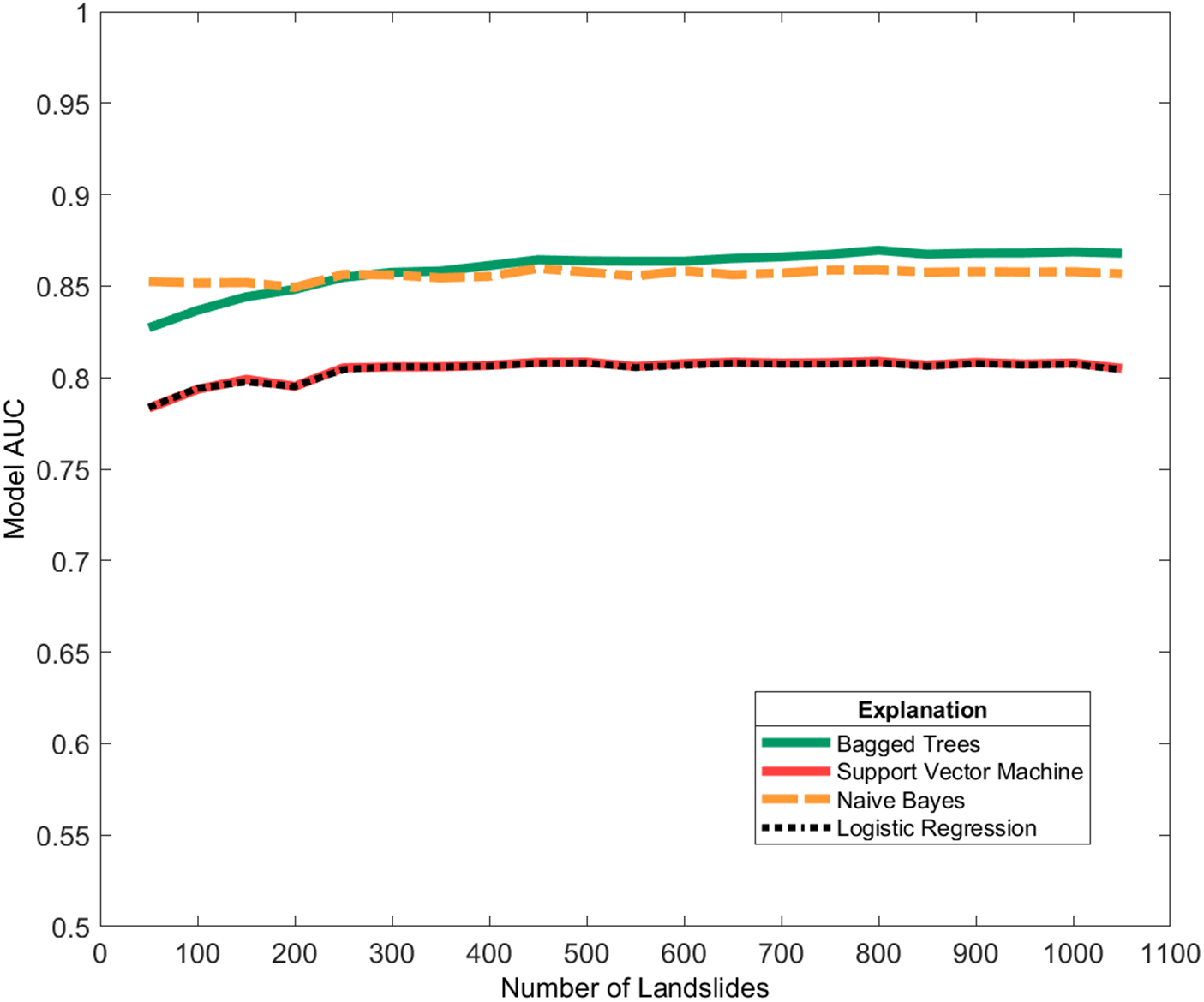
In the algorithm comparison test, ML algorithms performed similarly overall (Fig. 6). The LR and SVM had nearly identical mean AUC across increments. NB and BT had higher initial AUC but showed little improvement as the number of landslides increased.
Mean model AUC for 1000 iterations with increasing landslide inventory size in four typical machine-learning approaches. The logistic regression (LR) and support vector machine (SVM) models had nearly overlapping mean AUC. While the mean AUC for the Naïve Bayes (NB) and bagged trees (BT) models were initially higher than those of the LR and SVM models, they likewise did not improve dramatically with the inclusion of more landslides.

Much like the preliminary assessment, the mean AUC values for each ML algorithm appeared to improve with more data, then effectively plateaued after approximately 300 landslides. Plateaus were seen across all approaches, although some models achieved higher AUC values overall. The lack of correlation between AUC and increased inventory size hints at deeper complexities in the modeling approach despite which ML algorithm is chosen.
Feature selection
A majority of the 25 features were preserved by starting with a less stringent group ρ σgroup threshold (1.0). The large number of features led to model instability and rare logistic regression events. Thus, a stricter group ρ σgroup threshold was determined. The effects of ρ were quantified using thresholds ranging from 0.1 to 1 ρ at 0.1 increments on reduced Monte Carlo simulations (100 iterations) with AUC correction. The uncorrected AUC distributions for the model results indicated increased performance with higher (less stringent) thresholds and more features preserved; however, model results using cAUC (i.e., with correction factor) showed the highest and most stable performances at low ρ (more stringent) values (Fig. 7). We chose a threshold of 0.2 because it retained the most features before a precipitous drop in cAUC. Retaining as many layers as possible without significantly degrading performance is critical to capturing model result nuance (e.g., unimodal probability distribution instead of bimodal) and making more useful local susceptibility maps.
Results of threshold testing for the collinearity feature parsing. (a) Boxplots of 100 logistic regression (LR) iterations and their AUC distributions for each group ρ standard deviation threshold; (b) the same LR runs with distributions of the cAUC values from Eq. 5.; (c) the number of features included at each threshold. The dashed line represents the ρ standard deviation threshold chosen for the subsequent results. Green asterisks indicate outliers of the related boxplots.

Simulation results
The 0.2 ρ σgroup threshold omitted 19 of the original 25 statistical geomorphic features but improved the cAUC distributions compared to higher ρ σgroup thresholds. The seven retained features were mean aspect, sum curvature, minimum elevation, standard deviation elevation, standard deviation plan curvature, and standard deviation slope. In comparison, Crawford et al. (Reference Crawford, Dortch, Koch, Killen, Zhu, Zhu, Bryson and Haneberg2021) used the BT-based parsing methodology to yield 12 features for use in the LR, three of which were also retained in this study (sum curvature, standard deviation elevation, and standard deviation plan curvature).
Monte Carlo simulations with limited parsing and higher feature counts had less stable cAUC distributions compared to the reduced feature count simulations. That is to say, boxplots of the simulations with higher feature counts were characterized by more outliers, indicating that very few of the 1000 model iterations yielded useful maps (Fig. 8). Even after stability was reached through stricter feature parsing, at the maximum sample size, the cAUC values effectively ranged from 0.5 to 0.6 (∼10%; Fig. 9).
Boxplots for 1000-iteration Monte Carlo simulations of landslide inventory sizes tested using logistic regression and parsed with a ρ threshold of 1.0, which retained 23 features. (a) Uncorrected AUC distribution of the Monte Carlo simulation; (b) corrected AUC (cAUC) distribution. The thresholds for strong and moderate model performance are based on the AUC and cAUC thresholds shown in Table 1. Green asterisks indicate outliers of the related boxplots.

Boxplots for 1000-iteration Monte Carlo simulations of landslide inventory sizes tested using logistic regression and parsed with a ρ threshold of 0.2, which retained six features. (a) Standard distribution of the Monte Carlo simulation; (b) corrected AUC (cAUC) distribution. While the mean cAUC was initially very low for small landslide inventories, it stabilized rapidly at approximately 0.55 with an inventory size of only 200 landslides. Horizontal dashed lines represent thresholds for strong and moderate model performance based on typical AUC and cAUC divisions. By 350 landslides, model outliers were within the moderate performance zone. Green asterisks indicate outliers of the related boxplots.

Logistic regression map results
From the Monte Carlo simulations, the maximum and mean iterations for each sample size were calculated as county-wide susceptibility maps for visual inspection. Select sample sizes (50, 100, 500, and 1050 landslides) are shown in Figures 10 and 11. Figure 10 specifically highlights the map results (maximum AUC and maximum cAUC) from a minimally parsed feature pool, that of a ρ threshold of 1.0 (Fig. 8). While largely spurious and incomprehensible, output map results from the less parsed simulations are presented to emphasize the effectiveness of the correction and parsing methods. Figure 11 focuses on the parsed model (Fig. 9) and compares maximum AUC and maximum and mean cAUC values. With Figure 11 we show that with feature parsing and use of the correction, the mean cAUC and maximum cAUC were visually similar. While the distributions of the AUC values for the Monte Carlo iterations in the less-parsed models had mean values indicating strong model performances, Figure 10 details the lack of consistent or interpretable model results. Applying a correction factor for normality improved results but was overall ineffective with so many retained features, as the whole of the AUC/cAUC distribution produced incoherent model results despite good model performance. Figure 11 shows that with strict parsing, output maps were more visually realistic for both maximum uncorrected and corrected map results. Further, these maps were stable (largely unchanged and visually similar) for 500 or more landslides.
Landslide susceptibility maps for a small region in Magoffin County (location shown in Figure 1 inset). The maps display logistic regression probabilities from the unparsed Monte Carlo simulation iterations with the maximum AUC or maximum corrected AUC (cAUC) values for four select inventory sizes. AUC and cAUC values are shown in the upper right-hand corners of each map; probability distributions of county-level susceptibility are denoted by line graphs in the lower left-hand corners.

Landslide susceptibility maps for a small region in Magoffin County (location shown in Figure 1 inset). The maps display logistic regression probabilities from the strictly parsed (six retained features) Monte Carlo simulation iterations with the maximum AUC, maximum corrected AUC (cAUC), and mean cAUC values for four select inventory sizes. AUC and cAUC values are shown in the upper right-hand corners of each map; probability distributions of county-level susceptibility are denoted by line graphs in the lower left-hand corners. By 500 landslides, models are visually consistent with the full inventory for both AUC and cAUC.

Figure 11 also denotes the stability of results across the distribution of cAUC values, indicating that with correction and stricter feature parsing using the lower ρ threshold of 0.2, map variability was minimized across iterations of the larger sample sizes in the Monte Carlo simulation. In sum, stricter parsing led to more consistent map results and cAUC for landslide inventory sizes of 350 or greater, as shown in Figures 9b and 11.
Comparison with additional features
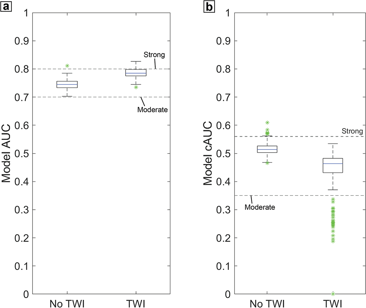
Using the full inventory (1054 landslides), TWI was added to the feature pool and the full workflow was run. The ρ threshold had to be manually increased to 0.3 because TWI features were otherwise omitted in the LR map making features. The results show that including TWI increased AUC but decreased cAUC compared to results without TWI (Fig. 12). This test validates both the choice of ρ and the necessity to apply corrections to AUC to determine the statistical significance and direction of change. The addition of TWI-based statistical geomorphic features did not yield a significant visual difference in the map results due to symbology. However, distinctions between the maps with and without TWI can be seen (Fig. 13), as many areas of lower probability without TWI increase to the highest probability category with TWI, indicating probability overprediction. The TWI-based workflow output maps show much sharper spatial contrast between areas of lower and higher probability due to the bimodal nature of the distribution. In general, more nuanced gradation between susceptibility classes lends towards better map utility (Crawford et al., Reference Crawford, Koch and Dortch2025). This approximation of expert preference by utilizing more normally distributed map results is correlated with tighter cAUC distributions, which suggest stronger performance.
Boxplots for 1000-iteration Monte Carlo simulations for the full inventory (1054 landslides) in a logistic regression with (a) an uncorrected AUC value distribution comparing models with and without topographic wetness index (TWI), and (b) a corrected AUC (cAUC) value distribution of the same TWI comparison. The lower cAUC value outliers are likely a result of too many features present. Thresholds for strong and moderate model performance were based on the AUC and cAUC thresholds shown in Table 1. Green asterisks indicate outliers of the related boxplots.

Landslide susceptibility maps for a small region in Magoffin County (location shown in Figure 1 inset). The maps display logistic regression probabilities from the best performing (maximum corrected AUC [cAUC]) Monte Carlo simulation iterations using feature pools with and without topographic wetness index (TWI). The cAUC values are shown in the upper right-hand corners of each map; probability distributions of county-level are denoted by line graphs in lower left-hand corners. When including TWI, there is in an increase in the total area of high probability; thus, the contrast between higher and lower landslide probabilities is much sharper.

Discussion
Interpretation of results
Inventory size
The motivating investigation using subsets of the Magoffin inventory (Fig. 3) detailed that the inclusion of more landslides did not make a statistically significant improvement to AUC past 300 landslides. This plateauing effect was also noted to some extent in both the AUC and cAUC value distributions for the larger sample sizes. Plateauing has been observed previously in similar studies of data effects (Heckmann et al., Reference Heckmann, Gegg, Gegg and Becht2014; Hussin et al., Reference Hussin, Zumpano, Reichenbach, Sterlacchini, Micu, van Westen and Bălteanu2015) and is not specific to landslide susceptibility modeling approaches (Stockwell and Peterson, Reference Stockwell and Peterson2002; Valavi et al., Reference Valavi, Guillera-Arroita, Lahoz-Monfort and Elith2022). We are unable to fully account for the accuracy plateau with an increase in landslide inventory size. Heckmann et al. (Reference Heckmann, Gegg, Gegg and Becht2014) showed in their own Monte Carlo simulation that additional landslide data yielded diminishing returns, attributing this to a breakdown in an autocorrelated range. Ultimately, Heckmann et al. (Reference Heckmann, Gegg, Gegg and Becht2014) recommended optimizing inventory size for usage in models.
The stabilization of model AUC and cAUC value distributions appears to match a rule-of-thumb estimate for minimum sample size based on the number of model features, as suggested by Green (Reference Green1991). Green (Reference Green1991) noted that 50 + 8x, where “x” represents the number of features, corresponds to the number of samples needed. Using this equation, an inventory size of 100 is needed for a model with six features. cAUC value distributions are less constrained at a sample size of 100 landslides (plus 100 non-landslides) than at larger sample sizes. Model performance began to fluctuate around a maximum cAUC with visually good (i.e., interpretable and close to normally distributed) maps starting around 500 landslides. With the correction and full feature parsing, a good map could be chosen with a minimum sample size as small as 100 landslides with our Monte Carlo approach; however, variance generally decreased as landslide inventory size increased, reaching a minimum variance of 10% with the full dataset. Mean AUC and cAUC both stabilized at approximately 350 landslides similar to the preliminary investigation (Fig. 3).
Box plot variability in Figures 8 and 9 clearly demonstrates that very small landslide inventory sizes do not produce stable map results, although the reduced variability of the AUC values in the increments ≥ 200 landslides does allude to some additional information provided by more landslide inventory data in our study area. As expected, 50 landslides are unable to produce a stable increment and subsequently useful output maps, even with correction. The minimum number of landslides needed to reach stability will likely vary between regions based on incision, steepness, sediment thickness, vegetation, climate, etc. Thus, we suggest that using an inventory that is as complete possible over varied terrain within the area of interest would be expected to yield more robust model results. Additionally, Figure 7 demonstrates that model AUC variability generally increased when more than six features were included. As models and features become more robust (i.e., using datasets not derived from a DEM that likely will pass the ρ threshold), the number of landslides required in an inventory may significantly increase before stabilizing. Ultimately, some variability in model results appears inherent in data sampling regardless of inventory size, thus there is a need to diversify the types of features used in the models or the quality of data (but not necessarily the number of examples) in the inventory.
Utility of feature parsing
Isolating the effects of ρ as a threshold for feature inclusion is an important step in LR analysis, demonstrated by Figure 6. It would be impractical to use too many features, the exact number seemingly variable, as highlighted by the probability distributions and maps of the unparsed Monte Carlo assessments. Our extreme case using 25 statistical geomorphic features showcases the utility of our workflow, as many researchers leverage some form of parsing technique. This level of feature parsing may be less important with other ML algorithms, such as various decision tree algorithms, but those approaches are less common in the landslide literature, and it is difficult to produce susceptibility maps from the results. While collinearity checking was effective when using DEM derivatives, we highlight the possibility that many more features may be retained if disparate features (i.e., not all DEM derivatives, such as soil thickness) are utilized. However, this may not be detrimental because disparate features may each be useful for fitting. If model results become overfit with the application of disparate features, other feature parsing techniques would need to be explored. DEM derivatives will likely remain important features due to the significance of high-quality DEMs and ease of generation in landslide susceptibility modeling (Brock et al., Reference Brock, Schratz, Petschko, Muenchow, Micu and Brenning2020). Despite the potential inflexibility of the collinearity parser, the presented feature parsing method still has utility as a parsing method for DEM derivatives.
Utility of correction factor
The boxplots of cAUC results demonstrate that the correction factor effectively isolated “rare logistic regression events,” which are quantitively demonstrated to be relatively common when many input features are selected. These spurious map results (i.e. rare logistic regression events) (King and Zeng, Reference King and Zeng2001) are likely not a result of imbalanced datasets. The datasets used in this study were specifically balanced, but when using the full suite of 25 statistical geomorphic features, the ML approaches may have overpredicted susceptibility. This corroborates observations made by other landslide researchers (Steger et al., Reference Steger, Brenning, Bell, Petschko and Glade2016; Lin et al., Reference Lin, Lima, Steger, Glade, Jiang, Zhang, Liu and Wang2021). Rare logistic regression events largely disappeared when using models with reduced features. The corrected ρ threshold boxplots were decisive in determining where model stability was the highest. cAUC values did not follow typical benchmarks for performance—AUC values less than 0.7 indicate poor performance and less than 0.50 indicate random chance. We suggest cAUC value thresholds based on accepted AUC thresholds multiplied by a minimum correlation (0.8); thus, a cAUC of 0.56 (0.8 × 0.7) would provide a serviceable baseline for “strong” susceptibility results (Table 1). Both the mean and maximum cAUC stabilize above this threshold for quality map results.
Assessment of methodology
Feature selection
Using the same data as this study, Crawford et al. (Reference Crawford, Dortch, Koch, Killen, Zhu, Zhu, Bryson and Haneberg2021) used a BT algorithm based parsing technique that reduced their LR features down to 12, with only eight used in map making. This produced similar map results, but the workflow requires use of an additional ML approach, in which the process of deciding which features are parsed can be uninterpretable and subject to data sub-setting variability. In contrast, the iterative collinearity check and feature removal based on quantitative assessment of the behavior of ρ used here led to quality results while maintaining interpretability. While BT may be more robust and is preferred by some researchers (Merghadi et al., Reference Merghadi, Yunus, Dou, Whiteley, ThaiPham, Bui, Avtar and Abderrahmane2020), this approach is still vulnerable to lack of interpretability due to its internal “black box” nature. Relatedly, Tsangaratos and Ilia (Reference Tsangaratos and Ilia2016) showed that NB achieved more stable results with less data, which is corroborated by this study (Fig. 6).
Despite these apparent improvements on LR and SVM, the BT and NB approaches experienced similar AUC plateaus as sample size increased. This workflow was calibrated using a limited pool of DEM-derived features. Susceptibility studies often focus on DEMs and their derivatives for generating model input data (Reichenbach et al., Reference Reichenbach, Rossi, Malamud, Mihir and Guzzetti2018), and Maxwell et al. (Reference Maxwell, Sharma, Kite, Donaldson, Maynard and Malay2021) indicated that accurate probabilistic slope failure maps did not need non-terrain-based features. Inclusion of non-DEM specific datasets, such as root strength index, has been noted to improve results by as much as 8% (Swallom et al., Reference Swallom, Koch, Dortch, Crawford, Thigpen and Andrews2025). However, these model improvements (like many others in the literature) may need to be reassessed using a workflow similar to that proposed here. With potential tweaking to the ρ threshold, features such as quantitative proxies of soil, lithology, and landcover can be included and tested for model improvement, in a similar fashion to TWI addition of this study (Figs. 12 and 13).
Correction factor
Our study demonstrates inherent data variability previously observed in the literature (Heckmann et al., Reference Heckmann, Gegg, Gegg and Becht2014) and presents a consistent method to select the most reasonable map. AUC is not the sole indicator of a good model (Lobo et al., Reference Lobo, Jiménez-Valverde and Real2007; Goetz et al., Reference Goetz, Brenning, Petschko and Leopold2015) and focusing on AUC can be detrimental to the production of realistic susceptibility maps. Expert opinion could be an alternative to AUC, but to identify the most realistic and accurate model among thousands, these subjective opinions would need to be objectively quantified. Crawford et al. (Reference Crawford, Koch and Dortch2025) showed that a more normally distributed map surpassed models with higher AUC values. Considering the timespan of these susceptibility maps based on the lack of age constraints, we found a normal distribution to be the best approximation for this inventory. Further, the input landslide inventories, even when derived from high-resolution LIDAR terrain interpretation, are likely not fully encompassing (Lima et al., Reference Lima, Steger and Glade2021). As such, when incomplete datasets are used, it is advisable to select a more stable (i.e., normally distributed) susceptibility map because incomplete datasets can yield significant biases (Steger et al., Reference Steger, Brenning, Bell, Petschko and Glade2016, Reference Steger, Brenning, Bell and Glade2017). Additionally, the normality-based correction factor cuts out the extreme probabilities in favor of non-extreme, more normal maps. Even if selected arbitrarily, the normal-distribution-based correction serves the purpose of a high- and low-probability filter, those end member probabilities that generally yield spurious maps despite high AUC values. AUC is widely recognized, generally interpretable, and calculatable; therefore, using an AUC-based correction factor increases the accessibility of the correction method.
We acknowledge that that a correction factor on model probabilities may cause model results to further deviate from true landslide probabilities as inferred from the inventory data. Because our workflow relies on comparison to an idealized probability distribution for the AUC correction, we started with a normal distribution as the benchmark. Note that despite choosing a normal distribution, the best performing cAUC maps have a minor to moderate positive skew, thus are not excluded (Fig. 11). Different comparative distributions could be explored further, but the literature provides little basis for distribution selection. Jai et al. (Reference Jia, Alvioli, Gariano, Marchesini, Guzzetti and Tang2021) found a positively skewed distribution inferred from global non-landslide areas; their observation could mean that a negatively skewed distribution would be a more suitable comparison probability distribution.
Observing that landslides are relatively sparse and unevenly distributed on the landscape (Huang et al., Reference Huang, Xiong, Jiang, Yao, Fan, Catani, Chang, Zhou, Huang and Liu2024), it may be that true static landslide susceptibility maps should highlight landslides on specific, relatively small portions of hillslopes. Therefore, the expected probability of a full landscape-scale landslide susceptibility distribution should be positively skewed toward the lower landslide probabilities that cover a majority of the landscape. Investigations into the optimal comparison probability distribution and its potential linkage to topography, lithology, average climate, and structure are left for future work.
Moreover, cAUC results may be low if the initial data/inventory are poorly behaved. The cAUC approach simply identifies the ‘best’ map of the iterations, which does not guarantee that it is good or realistic. Importantly, the baseline workflow presented here enables those future comparisons to be made by providing quantitative assessment of noise. By performing an AUC correction outside of the ML infrastructure, spurious and poor model results can be assessed and omitted in a systematic fashion. Further, application of a model correction factor can effectively identify features for omission (such as seen with our TWI test), leading to more realism and overall model stability. Detachment of the correction factor from the ML algorithm steps also avoids a workflow with a stronger stepwise approach. Stepwise LR, in which features are selected by additive t-testing within multiple LR, are sometimes used for data parsing (Van Den Eeckhaut et al., Reference Van Den Eeckhaut, Marre and Poesen2010; Heckmann et al., Reference Heckmann, Gegg, Gegg and Becht2014). Repeat feature selection and further data sampling are not uncommon (Beguería, Reference Beguería2006; Guns and Vanacker, Reference Guns and Vanacker2012). However, stepwise workflows are often considered by statisticians to be ineffective (Smith, Reference Smith2018). Thus, we avoided stepwise workflows for feature and ML algorithm selection, instead comparing the full Monte Carlo simulation for each algorithm type.
Sensitivity approach
Many published landslide susceptibility studies utilizing ML are likely unreproducible given the 10% model variance on our full inventory simulation, which is attributable to the selection of train and test data. Reproducibility could be increased through standard reporting of the seed used by random number generators in various software packages. However, a variety of software packages, many without access to seed-setting functionality, are used by the community, and the same seeds and programs would need to be used to achieve the same results. Only robust stochastic or brute force simulations would be able to assess the number of landslides in an inventory to consistently obtain the best models.
Model results centered near the means of the AUC value distributions also produced spurious results when using the full suite of 25 features. Figure 11 shows that the mean susceptibility map with six features is similar to, but less normally distributed than, the maximum cAUC map. This suggests that susceptibility models were roughly stable across the distribution due to workflow filtering components (i.e., ρ thresholds and AUC correction). It is impossible to determine where a single model run, without context, would fit into the larger potential distribution or to claim that any single model run is the most realistic map result. Significant variability is seen in similar models (Maxwell et al., Reference Maxwell, Sharma, Kite, Donaldson, Maynard and Malay2021; Crawford et al., Reference Crawford, Koch and Dortch2025), demonstrating that variability in results is not only possible but has potentially been incorrectly attributed to the inclusion of new layers or methods.
The addition of TWI test demonstrates the importance and practical application of the approach outlined in this study. Adding TWI increased AUC by 2%, which is significant even after accounting for noise (variance) due to selection within the landslide inventory. This apparent improvement is confirmed by findings from several studies (Jebur et al., Reference Jebur, Pradhan and Tehrany2014; Goetz et al., Reference Goetz, Brenning, Petschko and Leopold2015; Crawford et al., Reference Crawford, Koch and Dortch2025). However, when comparing cAUC values, including TWI significantly decreased performance of the best model and reduced mean cAUC by 5%. The implications of this result are that many commonly tested features may not increase model performance outside of noise, and features that increase AUC may make susceptibility maps look more unrealistic (i.e., lower cAUC).
Future work
Now that a quantitative workflow to establish the ‘best’ map selection and uncertainty has been identified, many previously modeled ideas on landslide parameter suitability and modeling approaches need to be reassessed. This includes map averaging, hyperparameter specifics, algorithm selection, feature parsing, and negative sampling approaches. For example, it may be useful to explore aggregating a subset of map results into a single map, such as a top quartile range of cAUC for each sample size. Aggregating a subset of results around either the mean or median (Heckmann et al., Reference Heckmann, Gegg, Gegg and Becht2014) would have been useful for AUC results but unnecessary for cAUC results because the correction factor removes extreme results.
Assessing the effects of landslide inventory size and feature selection in isolation potentially ignores a number of noteworthy model optimizations, such as hyperparameter specifications. The wide variety of hyperparameter specifications can increase with model complexity. For the LR model, hyperparameters are comparatively simple. However, hyperparameter variation was not done in this study because the number of models required for full assessment (21,000) would have increased exponentially (e.g., 21,000 × 30). However, it is possible to test models with complicated and significant hyperparameters using the workflow presented in this study to quantify the impact of hyperparameter settings. Algorithm selection considerations were also comparatively limited, we targeted specifically common and relatively simple algorithms to determine if there were differences to support our point that the issues presented are inherent in the data not in the algorithm. Specific modeling methods may be more robust against data variability (e.g., maximum entropy; Gomes et al., Reference Gomes, IJff, Raes, Amaral, Salamão, de Souza Coelho and de Almeida Matos2018; Pandey et al., Reference Pandey, Pourghasemi and Sharma2020; Valvai et al., Reference Valavi, Guillera-Arroita, Lahoz-Monfort and Elith2022) and targeted modeling frameworks that include hyperparameter considerations would also likely improve this workflow. An objective of this study was to quantify and account for variability from input inventory data. With that variability recognized, algorithm selection, hyperparameter testing, and input data differentiation can now be performed and accurately assessed for further model improvement. These tests do require a full simulation of the Monte Carlo workflow, to ensure that the changes in performance are not specific to a single train/test split.
Feature parsing was not performed on the individual subsamples of landslide data because this would have added complexity to the modeling workflow. Parsing techniques that depend on the data sampled are likely to be subject to the same variability observed in the model results, potentially at a larger scale. These assessments may continue progress towards representative landslide susceptibility models based on input data but may not lend towards modeling stability. Feature parsing based on random subsampling of the inventory will also likely be more sensitive to incomplete and inconsistent landslide inventories. Woodard and Mirus (Reference Woodard and Mirus2025) cited problems with landslide data limiting model performance. While this method attempts to control variability inherent in landslide datasets, further work on more robust characterization and parametrization of landslide inventories can only improve assessments like the one presented in this study.
In relation to landslide location inventory, the selection of non-landslide points can have a significant effect on model variability (Hu et al., Reference Hu, Zhou, Wang and Wang2020; Crawford et al., Reference Crawford, Koch and Dortch2025). Random selection of non-landslide points was used in this work, despite the existence of more robust approaches to non-landslide point selection (e.g., Huang et al., Reference Huang, Cao, Jiang, Zhou, Huang and Guo2020; Khabiri et al., Reference Khabiri, Crawford, Koch, Haneberg and Zhu2023; Zhou et al., Reference Zhou, Wang, Cao, Singh, Ahmed, Motagh, Wang, Chen, Tan and Li2024; Koch et al., Reference Koch, Haneberg, Crawford, Dortch and Swallom2025). A weakness of non-landslide point selection is the potential of sampling of a landslide, especially if the landslide has not been mapped. In this study, all non-landslide points were visually accessed, which showed <2% of non-landslide locations were near or overlapped with an existing landslide. However, landslide inventories are often noted to be incomplete (Steger et al., Reference Steger, Brenning, Bell, Petschko and Glade2016, Reference Steger, Brenning, Bell and Glade2017; Woodard and Mirus, Reference Woodard and Mirus2025), and in some cases may contain false positives. Until mapping can be more certain, and robust review of landslide inventories are widespread, selection of positive and negative samples likely will contribute a small fraction of errors. Ultimately, non-landslide locations are complex considerations and likely need a full comparison of different selection approaches using the Monte Carlo workflow presented in this study.
Conclusions
Much of landslide susceptibility modeling leverages ML algorithms, often without knowing the extent to which the results are affected by the input data. These input data effects can significantly affect the output models, reducing reproducibility, comparability, transferability, and the efficacy of landslide susceptibility models used by researchers interested in landscape evolution, local emergency managers, and other end users.
Presented in this study is a workflow to quantify and correct output model variability from the effects of input data. We leveraged a Monte Carlo sensitivity analysis on a LR-based susceptibility approach. Outside of the model, a rank correlation-based feature selection method was employed, as well as an AUC correction on the output LR results. This workflow, including the application of a correction factor and feature selection method, promoted stability and helped select realistic map results that may have been overlooked due to lower performance metrics.
This study highlights the difficulties associated with pursuing performance metrics without considering map utility, bringing attention to the importance of producing usable results even if the chosen model does not have the highest AUC. Moreover, a quantitative metric is still necessary to compare results of thousands of models both within and between study areas—our presented cAUC has the potential to fill that role. Other than circumventing AUC skew and yielding practical map results, this sensitivity analysis delineates a benchmark of noise from inventory effects alone. Further alterations to the modeling workflow can be assessed for significance by comparison to this baseline. Models need to be supported to minimize deviation and fully leverage the available data—our approach is a step in that direction.
Supplementary material
The supplementary material for this article can be found at https://doi.org/10.1017/qua.2026.10101.
Acknowledgments
Thank you to Bill Haneberg and Junfeng Zhu for critical questions and comments during the conceptualization of this workflow. Thank you to Meredith Swallom for the good suggestions and feedback on clarity. Thank you to Kentucky Geological Survey (KGS) editor Shelby Fulton for thorough and prompt review. Thank you to the anonymous reviewers and Quaternary Research editors for their suggestions and improvements. Thank you to National Science Foundation EPSCoR CLIMBS Project 2 (OIA 2344533) and KGS SP&M Lab for building capacity to run these memory-intensive simulations. This research was also supported by the Center for Land Surface Hazards (CLaSH), funded via National Science Foundation Cooperative Agreement EAR-2425607. We thank Stardust Dortch and Keiko Suzuki for feedback and support.
Author contributions
Conceptualization: H.J.K., J.M.D. Methodology: H.J.K., J.M.D., B.H. Software: H.J.K., J.M.D. Data Curation: H.J.K. Formal analysis: H.J.K Visualization: H.J.K Investigation: H.J.K., J.M.D. Validation: B.H. Resources: J.M.D. Supervision: J.M.D. Writing—Original draft: H.J.K., J.M.D. Writing—Review and editing: H.J.K., J.M.D., M.M.C., B.H.
Competing interests
The authors declare that they have no competing interests.






 Open access

