





Impact Statement
Atmospheric winds vary drastically in speed, direction and turbulence properties, significantly affecting wind turbine wakes – regions of slower-moving air behind the rotor. However, existing simulation approaches struggle to span the full complexity of these atmospheric conditions. We present a new method for simulating wake dynamics by prescribing a wind profile and layering turbulence and additional physics, such as Coriolis forces, giving full control over the incident wind. By analysing over 600 simulations, we isolate critical atmospheric processes that most strongly affect wake evolution. These insights provide a scalable framework for understanding wake physics across the wide range of conditions present in the atmosphere, which may lead to improved wake modelling and improved wind farm efficiency.
1. Introduction
Wind turbines, which extract energy and momentum from winds in the atmospheric boundary layer (ABL), cast wakes downstream. These energy-deficient regions negatively impact power production downwind, while elevated levels of turbulence may increase fatigue loading. Mitigating wake interactions within wind turbine arrays relies on understanding how energy and momentum are replenished into the wake region through turbulent mixing. However, wake transport mechanisms are affected by a large set of ABL processes, including wind shear and wind veer (vertical gradients of wind speed and wind direction, respectively), stratification, Coriolis forcing, mesoscale forcing, orography and diurnal and transient effects, to name a few (Landberg Reference Landberg2015). These properties of the ABL are often correlated, posing a challenge for studying each effect in isolation (cf. Kelly & van der Laan Reference Kelly and van der Laan2023; Türk & Emeis Reference Türk and Emeis2010). Additionally, mesoscale forcing and diurnal effects contribute to a high degree of variability for the inflow properties of the ABL, which are difficult to simulate with microscale large-eddy simulations (LES) or recreate in wind tunnel experiments (Haupt et al. Reference Haupt, Kosović, Berg, Kaul, Churchfield, Mirocha, Allaerts, Brummet, Davis, DeCastro, Dettling, Draxl, Gagne, Hawbecker, Jha, Juliano, Lassman, Quon, Rai and Thedin2023). As a result, the effects of individual, measurable properties of the ABL, such as wind veer, on the resulting wake dynamics have not been systematically identified in controlled tests.
Many previous studies have investigated ABL–wake interactions, most commonly through the concurrent-precursor method (Stevens et al. Reference Stevens, Graham and Meneveau2014). In the concurrent-precursor method, an empty domain is used to spin up a turbulent ABL inflow, which serves as the inflow condition to a second domain containing one or more wind turbines. A key focus of previous work has been the effects of turbulence intensity (
 $\mathrm{TI}$
) and wind shear on wake recovery in the ABL. For example, Wu and Porté-Agel (Reference Wu and Porté-Agel2012) used LES to investigate the effect of shear and
 $\mathrm{TI}$
by varying the roughness length
 $z_0$
in neutral boundary layers, finding that across the range of
 $\mathrm{TI}$
and wind shear studied,
 $\mathrm{TI}$
has a strong effect on wake recovery, while the effect of wind shear on wake recovery is comparatively negligible. These conclusions are corroborated by other numerical studies (Chu & Chiang Reference Chu and Chiang2014; Churchfield et al. Reference Churchfield, Lee, Michalakes and Moriarty2012) and wind tunnel studies (Bartl et al. Reference Bartl, Mühle, Schottler, Sætran, Peinke, Adaramola and Hölling2018; Chamorro & Porté-Agel Reference Chamorro and Porté-Agel2009). Several LES studies have investigated the effects of stratification on wake development (Abkar & Porté-Agel Reference Abkar and Porté-Agel2015; Churchfield et al. Reference Churchfield, Lee, Michalakes and Moriarty2012), finding that under convective conditions, vertical meandering and wake recovery are enhanced, while under stably stratified conditions, wake spreading and recovery are suppressed. However, wind shear, inflow
 $\mathrm{TI}$
and turbulence length scales are simultaneously affected when varying the background stratification. To disentangle these effects, Du et al. (Reference Du, Ge, Zeng, Cui and Liu2021) strategically varied
 $z_0$
and the domain height
 $L_z$
in concurrent-precursor LES to match the hub height wind speed
 $U_h$
and
 $\mathrm{TI}$
across stable, neutral and unstable (convective) conditions. As a result, they concluded that larger turbulence length scales were responsible for faster wake recovery in convective conditions, relative to neutral conditions, despite lower shear, and vice versa in stable conditions. Similarly, increasing turbulence length scales were found to increase wake recovery in wind tunnel experiments and LES by España et al. (Reference España, Aubrun, Loyer and Devinant2011) and Vahidi & Porté-Agel (Reference Vahidi and Porté-Agel2024), respectively, and to promote wake meandering in wind tunnel experiments (Bourhis et al. Reference Bourhis, Messmer, Hölling and Buxton2025).
Efforts to perform controlled experiments of ABL inflow properties are further complicated by the introduction of Coriolis forces. Xie & Archer (Reference Xie and Archer2017) investigated the effects of stratification across unstable, neutral and stable conditions with the inclusion of Coriolis forces in a five-turbine wind farm. They found similar power losses due to wake effects between neutral and stable conditions, but decreased power losses due to enhanced wake recovery in convective conditions. However, they noted many differences in inflow properties resulting from varying the stratification, including hub height velocity,
 $\mathrm{TI}$
, length scales and wind shear and veer. Other LES studies have observed that introducing Coriolis forces results in enhanced wake recovery, relative to an inflow without Coriolis forces, due to the presence of wind veer (Abkar & Porté-Agel Reference Abkar and Porté-Agel2016; Churchfield & Sirnivas Reference Churchfield and Sirnivas2018). Klemmer & Howland (Reference Klemmer and Howland2024) found that in stably stratified ABLs, wind shear and veer significantly alter turbulence and momentum budgets in the wake, enhancing the additional turbulence generated by the turbine wake relative to neutral ABLs. Several studies have also noted that the indirect effects of stability on the inflow, such as through wind shear, veer and turbulence length scales, have a more pronounced effect on the wake dynamics than the direct buoyant production/suppression of turbulence kinetic energy (Du et al. Reference Du, Ge, Zeng, Cui and Liu2021; Klemmer & Howland Reference Klemmer and Howland2024, Reference Klemmer and Howland2025). In neutral ABLs, Heck & Howland (Reference Heck and Howland2025) found that changing the relative strength of Coriolis forcing had a minimal impact on the wake recovery rate, but significantly affected the magnitude and direction of ABL inflow-induced wake deflections depending on incident conditions. Other studies have also observed competing effects of Coriolis forces on wake deflections (cf. Gadde & Stevens Reference Gadde and Stevens2019; Howland et al. Reference Howland, Ghate and Lele2018; van der Laan & Sørensen Reference van der Laan and Sørensen2017). Clearly, the properties of the ABL inflow can have a substantial influence on wind turbine wake dynamics, but studying the effects of each parameter in isolation poses many challenges due to the coupled nature of ABL processes. Meanwhile, the wide range of stratification, surface morphology (roughnesses) and large-scale weather conditions that are present in real ABLs causes a significant spread in these inflow parameters that cannot all be reliably produced by a microscale LES model in isolation.
Mesoscale-to-microscale coupled (MMC) simulations introduce transient dynamics and large-scale weather patterns into the LES flow, disrupting the correlated nature of flow variables in microscale simulations, such as wind shear and wind veer (Landberg Reference Landberg2015). As a result, a wider variety of wind conditions can be simulated in MMC simulations compared with microscale LES alone. For example, Wise et al. (Reference Wise, Neher, Arthur, Mirocha, Lundquist and Chow2022) used MMC simulations to investigate wind turbine wakes over a mountain ridge in stable and convective conditions. Those authors found that in stable conditions, wakes follow the terrain contours, but in convective conditions, wakes are carried aloft. Recently, Chatterjee et al. (Reference Chatterjee, Jayaraman, Yellapantula and Quon2025) used coupled simulations to investigate the impact of low-level jets on wind farm performance. While MMC simulations are useful for case studies and faithful reconstruction of atmospheric dynamics, they have limitations. In addition to the elevated computational cost of performing nested-domain simulations, synthetic turbulence perturbation methods are critical to reconstructing the spectral content in the microscale domain (Muñoz-Esparza et al. Reference Muñoz-Esparza, Kosović, Mirocha and van Beeck2014, Reference Muñoz-Esparza, Kosović, van Beeck and Mirocha2015). Furthermore, the added complexity of the multi-scale coupling can result in a loss of controllability for simulating a target inflow profile, and the transient nature of MMC simulations limits the usefulness of turbulence statistics and budgets.
Synthetic inflow generation is another alternative to studying ABL–wake interactions across inflow conditions. Often, a mean wind-speed profile is prescribed with turbulent perturbations superimposed, and a region of the streamwise domain is allotted to flow adjustment for the turbulence to equilibrate (Troldborg et al. Reference Troldborg, Sørensen, Mikkelsen and Sørensen2014). The injected turbulence may derive from a precursor simulation, from forced homogeneous, isotropic turbulence (HIT), or from synthetic turbulence-generation methods, such as the Mann method (Mann Reference Mann1998) or the divergence-free synthetic eddy method (Poletto et al. Reference Poletto, Craft and Revell2013). Several studies have used synthetic turbulence generation to study wake dynamics separate from the ABL (e.g. Keck et al. Reference Keck, Mikkelsen, Troldborg, de Maré and Hansen2014; Doosttalab et al. Reference Doosttalab, Siguenza-Alvarado, Pulletikurthi, Jin, Evans, Chamorro and Castillo2020; Ghate et al. Reference Ghate, Ghaisas, Lele and Towne2018; Li et al. Reference Li, Dong and Yang2022; Li & Yang Reference Li and Yang2024). For example, Troldborg et al. (Reference Troldborg, Sørensen, Mikkelsen and Sørensen2014) found excellent agreement between field measurements of a wind turbine wake taken by meteorological masts and a synthetic ABL inflow using the Mann turbulence method. However, no studies have extended the synthetic ABL methodology to include additional properties of the inflow beyond wind-speed shear.
In this study, we propose a synthetic inflow approach to studying ABL–wake physics across broad ranges of wind shear, wind veer, Coriolis forcing and turbulence parameters. In prescribing a mean wind-speed profile, we decouple the inflow shear from the effects of the wall (prescribed here as a slip wall) and therefore the mechanism for turbulence generation. Instead, turbulence is injected into the domain at the inlet with a prescribed integral length scale and
 $\mathrm{TI}$
. The wind direction profile is also prescribed, decoupling the wind veer from the combined effects of stratification, Coriolis forcing and wind shear. We first verify that the synthetic inflow approach reproduces the wake structure and dynamics present in concurrent-precursor simulations of wind turbine wakes immersed in stratified ABLs. Using this methodology, we can, for the first time, explore the impact on wake dynamics from shear, veer and other ABL parameters independently.
The remainder of the article is organised as follows. In § 2, we introduce the synthetic inflow methodology and the LES numerical set-up. We define a wake momentum budget that is used both for method verification and for flow physics analysis. To guide the regimes investigated in the LES cases, we investigate a range of ABL parameters observed at a field site on the north Atlantic coast of the United States. Beginning in § 3, we verify the synthetic inflow method against simulations of wakes immersed in ABLs simulated with a concurrent-precursor set-up. Then, in § 4, we use the new LES methodology to explore a wide range of parameters to identify key variables that have the greatest impact on wind turbine wake evolution. Finally, conclusions and opportunities for future work are summarised in § 5.
2. Methodology
In this section, we first introduce the LES numerical set-up and the synthetic inflow methodology in § 2.1. The momentum budget analysis, which is used to validate the synthetic turbulence inflow method and also to analyse the evolution of wakes as a function of inflow parameters, is described in § 2.2. Then, we outline a parametrisation of inflow wind shear and wind veer in § 2.3. Finally, in § 2.4, we describe the field data used to motivate the range of inflow parameters that are studied using the synthetic inflow method in this work.
2.1. Large-eddy simulation set-up
The open-source, pseudo-spectral LES code PadéOps (https://github.com/Howland-Lab/PadeOps) is used to solve the incompressible, filtered Navier–Stokes equations with the Boussinesq approximation for buoyancy using a coupled prognostic equation for potential temperature (Ghate & Lele Reference Ghate and Lele2017; Heck & Howland Reference Heck and Howland2025). Fourier collocation is used in the horizontal directions, and a fringe region (Nordström et al. Reference Nordström, Nordin and Henningson1999) is used in the streamwise direction to allow for finite-length wakes and to enforce inflow boundary conditions. A sixth-order-accurate Padé scheme is used for vertical differencing (Lele Reference Lele1992), and the bottom and top boundary conditions are slip walls with a no-flux condition. Time integration uses a fourth-order Runge–Kutta scheme.
To investigate a wide range of combinations of TI, wind shear, wind veer and Coriolis forcing in the ABL, idealised, synthetic inflow profiles are generated to approximate ABL inflows. The mean wind speed and direction profiles in the idealised simulations are prescribed by the methodology outlined in § 2.3. The geostrophic pressure gradient is varied as a function of
 $z$
to maintain consistency with the imposed velocity profile, thereby mitigating inflow adjustment. As the top and bottom boundaries are slip walls, turbulence must be injected into the domain, which is forced through a concurrently run simulation of forced HIT. Turbulence is introduced by superimposing the prescribed mean wind profiles with the HIT wind fields, which are phase-shifted to advect the turbulent fluctuations by the mean velocity as a function of
 $z$
. Furthermore, the turbulent fluctuations are bandpass-filtered by a prescribed high-pass filter of wavelength
 $\lambda _{{BP}}$
to adjust the integral length scale (Ghate et al. Reference Ghate, Ghaisas, Lele and Towne2018). A schematic for the modified concurrent LES set-up is shown in figure 1, and specific technical details on the implementation are described in Appendix A.
The LES methodology for the synthetic inflow simulations. Three LES are concurrently run (HIT, empty, primary), and the velocity perturbations from the HIT simulation are advected and superimposed on the mean profiles in the primary and empty domains.

Figure 1 Long description
Upper right panel: A heat map showing the velocity distribution in an empty simulation. The x-axis represents the distance normalized by the turbine diameter (x/D) ranging from -10 to 20. The y-axis represents the normalized velocity (u/Uh) ranging from 0.5 to 1.5. The colour scale indicates the velocity magnitude, with lighter colours representing higher velocities and darker colors representing lower velocities. The region labeled TI measurement shows where turbulence intensity is measured. The slip walls are indicated on the right side of the heat map. Upper left panel: A heat map showing the velocity distribution in a primary simulation with a turbine. The x-axis represents the distance normalised by the turbine diameter (x/D) ranging from -10 to 20. The y-axis represents the normalised velocity (u/Uh) ranging from 0.5 to 1.5. The colour scale indicates the velocity magnitude, with lighter colours representing higher velocities and darker colours representing lower velocities. The slip walls are indicated on the right side of the heat map. The PI controller and fringe regions are marked on the left side of the heat map. Left panel: a square heat map showing the velocity distribution in an empty simulation of forced homogeneous, isotropic turbulence. Arrows show the turbulence inputted to both the empty and primary simulations.
Turbulence will evolve as it is advected downstream (Keck et al. Reference Keck, Mikkelsen, Troldborg, de Maré and Hansen2014). For example, the TI prescribed at the inlet of the simulation will decay away with downstream distance under uniform inflow conditions (cf. Comte-Bellot & Corrsin Reference Comte-Bellot and Corrsin1966), but it could increase with downstream distance if the inflow speed or direction shear is sufficiently high, driven by shear production. To achieve a specified TI at the rotor disk, a closed-loop proportional–integral (PI) controller is used that measures the turbulence at the location of the turbine in a concurrently run empty domain simulation with no turbine. The closed-loop PI controller is robust across inflow conditions and is switched off once the desired TI at the location of the actuator disk becomes quasi-steady, as measured in the empty domain simulation. That is, the PI controller is turned off before any statistics are computed. Controller specifics and implementation are also further described in Appendix A. Finally, the empty simulation is used to compute on-the-fly deficit statistics (Klemmer & Howland Reference Klemmer and Howland2024), further described in § 2.2.
For the primary and empty simulations, the domain size is
 $10\pi D \times 4\pi D \times 2\pi D$
, and contains
 $480 \times 192 \times 96$
points in the streamwise (
 $x$
), lateral (
 $y$
) and vertical (
 $z$
) directions, respectively. This results in an isotropic grid with a grid size of
 $\varDelta \approx 0.065D$
. The rotor diameter
 $D$
is arbitrary because there is no other length scale in the simulation set-up (e.g. surface roughness; ABL height). A transient spin-up time of 16 flow-through times is used in all simulations to allow wakes to develop and for the TI controller to reach equilibrium. After the initial spin-up, flow statistics are time-averaged for 24 flow-through times for wake statistics to converge.
An irrotational actuator disk model (ADM) is used in all simulations to create a wake. The ADM is placed
 $x = 5D$
downstream of the domain inlet to allow the flow to develop from the inflow condition, and to accommodate the induction zone of the wind turbine. The turbine is centred laterally in the domain, and the hub height is
 $z_h/D = 0.625$
, which corresponds to
 ${150}\,\textrm {m}$
for the IEA 15 MW reference turbine (Gaertner et al. Reference Gaertner, Rinker, Sethuraman, Zahle, Anderson, Barter, Abbas, Meng, Bortolotti, Skrzypinski and Scott2020). The magnitude of the thrust force of the turbine
 $F_T = ( 1/2) \rho \pi R^2 u_d^2 C_T'$
is computed based on the disk-averaged velocity
 $u_d$
, where
 $R = D/2$
is the turbine radius and
 $C_T' = 4/3$
is the local thrust coefficient, corresponding to
 $C_T = 0.75$
(Calaf et al. Reference Calaf, Meneveau and Meyers2010) in shear-free, uniform inflow conditions. The correction factor introduced by Shapiro et al. (Reference Shapiro, Gayme and Meneveau2019) is used in all simulations, except when comparing with the truly neutral boundary layer (TNBL) cases from Heck & Howland (Reference Heck and Howland2025), because they did not use the Shapiro correction factor in their simulations. While we do not include wake rotation in this study, we note that previous studies have observed that interactions between wake rotation and wind veer cause significant changes to wake evolution (Englberger et al. Reference Englberger, Dörnbrack and Lundquist2020), which we recommend continuing in future work using the synthetic inflow method.
2.2. Momentum budget and streamtube analysis
In this study, we describe the dynamics of the wake using a prognostic equation for the wake velocity deficit. This double decomposition, originally introduced by Martínez-Tossas et al. (Reference Martínez-Tossas, King, Quon, Bay, Mudafort, Hamilton, Howland and Fleming2021), was expanded in Klemmer & Howland (Reference Klemmer and Howland2024) to include the wake-added turbulence kinetic energy budget. An abbreviated derivation is given here with further discussion in Klemmer & Howland (Reference Klemmer and Howland2024).
Beginning with the filtered, incompressible Navier–Stokes equations, we introduce the wake decomposition
 $u_i = u_i^B + \Delta u_i$
to parse the wake into the base flow (denoted with a superscript
 $B$
) and the deficit (wake) flow (denoted with
 $\Delta$
). Then, introducing the Reynolds decomposition, both the base flow and the deficit flow are further split into time-mean and fluctuating components:
 \begin{align} u_i^B &= \overline {u_i^B} + {u_i^B}', \\[-10pt] \nonumber \end{align}
 \begin{align} \Delta u_i &= \overline {\Delta u_i} + \Delta u_i'. \\[10pt] \nonumber\end{align}
We then substitute the double decomposition into the filtered, incompressible Navier–Stokes equations, Reynolds-average and assume statistical stationarity to remove the temporal derivatives, resulting in the full Reynolds-averaged Navier–Stokes (RANS) equations. Then, because the base flow must also satisfy the RANS equations, we subtract off the base-flow RANS equations from the full RANS to arrive at an equation for wake velocity deficit:
 \begin{align} \underbrace {{\vphantom {\frac {\overline {u_i'}}{x_j}}} (\overline {u_j^B} + \overline {\Delta u_j}) \frac {\partial \overline {\Delta u_i}}{\partial x_j}}_{\mathrm{Advection}} = \underbrace {{\vphantom {\frac {\overline {u_i'}}{x_j}}} -\frac {\partial \overline {\Delta p}}{\partial x_i}}_{\mathrm{Pressure\,grad.}} + \underbrace {{\vphantom {\frac {\overline {u_i'}}{x_j}}} \frac {\delta _{i3}}{\theta _0 Fr^2} \overline {\Delta \theta }}_{\mathrm{Buoyancy}} \underbrace {{\vphantom {\frac {\overline {u_i'}}{x_j}}} + \frac {1}{Ro}\varepsilon _{ij3} \overline {\Delta u_j}}_{\mathrm{Coriolis}} \underbrace {{\vphantom {\frac {\overline {u_i'}}{x_j}}} - \frac {\partial \overline {\Delta \tau _{ij}}}{\partial x_j}}_{\mathrm{SGS}} \underbrace {{\vphantom {\frac {\overline {u_i'}}{x_j}}} - \overline {\Delta u_j}\frac {\partial \overline {u_i^B}}{\partial x_j}}_{\mathrm{Base\,advection}} \underbrace {{\vphantom {\frac {\overline {u_i'}}{x_j}}} - \frac {\partial \Delta \overline {u_i' u_j'}}{\partial x_j}}_{\mathrm{Reynolds\,stresses}}. \\[-30pt] \nonumber \end{align}
Here
 $\Delta p$
is the wake-induced pressure field,
 $\Delta \theta$
is a wake-induced perturbation to the potential temperature,
 $\Delta \tau _{ij}$
represents the wake-added subgrid stresses (SGS) and
 $\Delta \overline {u_i' u_j'} \equiv \overline {u_i' u_j'} - \overline {{u_i^B}' {u_j^B}'}$
is the wake-added Reynolds stress tensor (Klemmer & Howland Reference Klemmer and Howland2024). Note that in (2.3), only the vertical component of Earth’s rotation is included (Howland et al. Reference Howland, Ghate and Lele2020
Reference Howland, Ghate and Lelea
), and the Rossby number is defined as
 $Ro = U_h/(f_c D)$
, where
 $U_h$
is the hub-height velocity and
 $f_c = 2\omega \sin (\phi )$
is the Coriolis parameter, where
 $\phi$
is the latitude and
 $\omega = {7.29\times {10}^{-5}}\,\textrm {rad s}^{-1}$
is the rotation rate of Earth. The Froude number
 $Fr = U_h/\sqrt {gD}$
is used in the stratified simulations in § 3.3, where
 $g = {9.81}\,\textrm {m}\, \textrm{s}^{-2}$
is the gravitational acceleration.
To facilitate the analysis of the wake physics, a streamtube (Meyers & Meneveau Reference Meyers and Meneveau2013) is used to spatially aggregate wake velocities, wake momentum budget terms in (2.3) and identify the wake centroid location (Heck & Howland Reference Heck and Howland2025). Tracking a streamtube selects a three-dimensional region that represents the wake robustly even in cases of inflow wind shear and wind veer. Throughout this study, we seed the streamtube at a radius
 $R_s = 0.7R$
in the rotor plane to avoid any Gaussian smoothing at the edges of the ADM (Heck et al. Reference Heck, Johlas and Howland2023; Shapiro et al. Reference Shapiro, Gayme and Meneveau2018). Streamtube-averaged quantities are denoted by
 $\langle \cdot \rangle$
, and are averaged within the streamtube region in the lateral (
 $y$
) and vertical (
 $z$
) directions.
2.3. Atmospheric boundary layer representation
The time-mean inflow profiles are prescribed as inputs to the simulation methodology introduced in § 2.1. In this study, inflow profiles of streamwise (
 $u$
) and lateral (
 $v$
) velocity depend only on the vertical coordinate
 $z$
, and the vertical inflow velocity (
 $w$
) is zero. We consider two sources of inputs for the mean inflow profiles. First, to verify the synthetic inflow method against concurrent-precursor simulations of wakes in the ABL, we prescribe the synthetic inflow with the exact mean profiles from the ABL precursor simulations. In this set-up, the primary remaining difference in the turbulent inflow of the synthetic inflow LES and the concurrent-precursor LES is the structure of the turbulence (length scales, anisotropy, etc.). Second, to investigate a wide range of inflow profiles, we prescribe an idealised parametrisation of wind speed and wind direction profiles. The parametrised inflow enables efficient simulation of wind turbine wakes subjected to independently varying wind shear and wind veer strengths.
The idealised profiles parametrise the mean wind speed
 $U = (\bar {u}^2 + \bar {v}^2)^{1/2}$
and mean wind direction
 $\psi = \arctan (\bar {v}/\bar {u})$
with the following expressions:
 \begin{align} U(z)/U_h &= 1 + (1-\epsilon ) \tanh \left (\frac {\alpha _s(z - z_{h})}{D(1-\epsilon )}\right ); & \psi (z) &= (1-\epsilon ) \tanh \left ( -\frac {\alpha _v(z - z_{h})}{D(1-\epsilon )}\right ). \end{align}
Here,
 $U_h$
is the wind speed at hub height
 $z_h$
. The variables
 $\alpha _s$
and
 $\alpha _v$
control the vertical gradients of wind speed (shear) and wind direction (veer), respectively. Near
 $z = z_h$
,
 $\tanh (x) \approx x$
and thus the profiles are approximately linear across the rotor extent:
 $U(z)/U_h \approx 1 + \alpha _s (z-z_h)/D$
and
 $\psi (z) \approx -\alpha _v (z-z_h)/D$
. Note that
 $\alpha _v \gt 0$
corresponds to positive wind veer, where
 $\psi$
decreases as a function of height in the northern hemisphere following the Ekman spiral. Away from the rotor, the wind speed and direction smoothly transition to a constant value set by a regularisation parameter
 $\epsilon = 0.2$
to prevent reverse flow in the LES. Empirically, wind profiles are often approximately linear in the ABL (Debnath et al. Reference Debnath, Moriarty, Krishnamurthy, Bodini, Newsom, Quon, Lundquist, Letizia, Iungo and Klein2023; Kelly & van der Laan Reference Kelly and van der Laan2023). Choosing approximately linear profiles for the wind speed is useful because in the ABL, vertical profiles of velocity may be quite complex, departing significantly from canonical profile shapes (e.g. power-law) due to diurnal effects, terrain, mesoscale forcing, etc. (Howland et al. Reference Howland, González, Martínez, Quesada, Larrañaga, Yadav, Chawla and Dabiri2020
Reference Howland, González, Martínez, Quesada, Larrañaga, Yadav, Chawla and Dabirib
). An effective parametrisation of non-logarithmic or power-law profiles (e.g. low-level jets) that depends on only one or two parameters could be utilised in future work with the same LES methodology.
2.4. Range of atmospheric profile parameters and LES inputs
In this study, we explore wake dynamics under realistic distributions of wind shear and veer observed in field measurements. Field data from a profiling lidar at the Martha’s Vineyard Coastal Observatory (MVCO) are used to assess distributions of ABL parameters (Bodini et al. Reference Bodini, Lundquist and Kirincich2020; Klemmer et al. Reference Klemmer, Condon and Howland2024; Lundquist & Zalkind Reference Lundquist and Zalkind2023). We use data from 2017, but the joint distributions do not change significantly for the years between 2017 and 2020 (not shown). In this study, we chose four non-dimensional parameters relevant to modern offshore wind turbines, based on previous literature outlined in the introduction regarding the key ABL parameters that affect wake dynamics, using the dimensions of the IEA 15 MW wind turbine for reference (Gaertner et al. Reference Gaertner, Rinker, Sethuraman, Zahle, Anderson, Barter, Abbas, Meng, Bortolotti, Skrzypinski and Scott2020). The parameters of choice are the Rossby number
 $Ro = U_h/(f_c D)$
, where
 $f_c$
is the Coriolis parameter, the hub-height turbulence intensity (TI
 $\equiv \sqrt {2k/3}/U_h$
, where
 $k$
is the turbulence kinetic energy), rotor-averaged wind shear
 $\alpha _s$
and rotor-averaged wind veer
 $\alpha _v$
. Note that definitions of
 $\alpha _s$
and
 $\alpha _v$
are fitted using the parametrisation in (2.4
 $a$
,
 $b$
), respectively, where wind direction profiles are unwrapped from the original circular domain of
 $[0^\circ , 360^\circ )$
. These parameters are computed from the field data, located at a latitude
 $\phi = 41.4^\circ$
N. Lidar TI (Bodini et al. Reference Bodini, Lundquist and Kirincich2020) is interpolated to hub height, as is the wind speed
 $U_h$
. The resulting distributions of non-dimensional inflow variables are shown in figure 2.
Joint distributions of observed ABL parameters at the MVCO and profiling lidar. Shear and veer distributions are approximated as linear profiles of wind speed and direction computed across the rotor extent, while
 $\mathrm{TI}$
is interpolated at hub height. The Rossby number is based on the turbine diameter of the IEA 15 MW reference turbine.

Figure 2 Long description
A triangular arrangement of 10 subfigures depicts the probability density function and joint distributions of variables labeled “shear”, “veer”, “Ro” (Rossby number), and “TI” (turbulence intensity). Filled contours of the joint probability density maps show increasing probability density levels with increasingly lighter colours. A lightly shaded blue box in each subfigure denotes the range of each variable that is investigated in the study.
An IEA 15 MW reference turbine located at the field data site would operate, on average, in slightly sheared (0.16) and veered (
 ${8.8}^{\circ }$
) conditions at relatively low TI (
 $5.6\,\%$
) and a Rossby number of
 $\approx 470$
. However, high magnitudes of wind shear (over 0.5, i.e. 50 % variation in wind speed across the rotor) and wind veer (over
 $30^\circ$
across the rotor) are also common. Furthermore, the joint distribution of variables shows a wide spread in combinations of all variables, including shear and veer. The shaded regions indicate the ranges of ABL parameters chosen to simulate using LES. Specific values of
 $\alpha _s$
,
 $\alpha _v$
,
 $Ro$
and
 $\mathrm{TI}$
, as well as the turbulence length scale, which we control with the high-pass filter scale
 $\lambda _{{BP}}/D$
(not estimated with the lidar profiles in figure 2), are given in table 1. We choose a wide range of reasonable offshore turbulence intensities to simulate, recognising uncertainties associated with inferring turbulence kinetic energy from lidar measurements (Bonin et al. Reference Bonin, Aditya Choukulkar, Sandberg, Weickmann, Pichugina, Banta, Oncley and Wolfe2017).
Parameters defining four full-factorial LES sweeps (i.e. all combinations are simulated) used in the exploration of ABL effects on wake evolution in § 4. Variable increments are evenly spaced (denoted with ‘
 $\ldots$
’) unless specific values are listed.

Table 1 Long description
The table presents parameters defining four full-factorial LES sweeps used in the exploration of ABL effects on wake evolution. It includes four rows and seven columns. The columns are labeled Sweep, Shear, Veer (deg.), Ro, TI (percent), lambda_BP/D, and Cases. Row 1: Sweep A, Shear -0.15, 0, ..., 0.6, Veer -10, 0, ..., 40, Ro 125, 400, 1000, TI 3, 8, lambda_BP/D 2 pi/3, Cases 216. Row 2: Sweep B, Shear 0, Veer 0, 10, 20, 30, Ro 1000, TI 2.4, ..., 10, lambda_BP/D pi/3, 2 pi, Cases 40. Row 3: Sweep C, Shear -0.1, -0.05, ..., 0.2 and ±0.02, Veer -10, -5, ..., 20 and ±2, Ro 100, 1000, TI 3, 8, lambda_BP/D 2 pi/3, Cases 324. Row 4: Sweep D, Shear -0.08, -0.02, 0.12, 0.25, Veer -6, 6, 18, Ro 80, 111, 167, 400, 2000, TI 4, lambda_BP/D 2 pi/3, Cases 60.
The four full-factorial parameter sweeps focus on different parameter regimes. Sweep A spans the widest range of shear and veer, while Sweep B spans the widest range of TI and turbulence length scales. Sweep C has a high granularity in shear and veer, but over a smaller range of values. Finally, Sweep D has a high granularity and a wide range of Rossby numbers. In total, these four sweeps constitute 640 synthetic turbulent inflow LES cases. Running on the Intel Xeon CPU MAX 9480 on the Stampede3 supercomputer, we find that the computational cost of one synthetic simulation is around
 $2000$
CPU hours, which is eight times cheaper than comparative concurrent-precursor simulations in the stratified boundary layer (SBL) (§ 3.3), and about 100 times cheaper than the grid-refined SBL simulations in Appendix B. The decreased cost of the synthetic simulations is a result of a drastically decreased spin-up time and smaller and coarser vertical grids, as the full ABL extent does not need to be simulated.
3. Wake comparison between synthetic and ABL profiles
In this section, we compare the wake dynamics in the synthetic inflow LES framework introduced in § 2.1 to simulations of wakes using the concurrent-precursor method (Heck & Howland Reference Heck and Howland2025), varying the Rossby number between
 $Ro = 100 \text{ and } 1000$
. First, in § 3.1, we compare the wake recovery, deflection and momentum deficit budgets across TNBL (also known as the turbulent Ekman layer) inflow conditions and Rossby numbers. Then in § 3.2, we use the synthetic inflow methodology to examine how integral length scales of turbulence impact wake evolution. Finally, in § 3.3, we compare the synthetic inflow methodology with concurrent-precursor simulations of wakes immersed in stably SBL inflow conditions.
3.1. Wake recovery, deflection and deficit budgets
To verify the proposed synthetic inflow methodology, we simulate a single wind turbine wake in turbulent inflow. The concurrent-precursor TNBL simulations in Heck and Howland (Reference Heck and Howland2025) are used as a reference, where the Rossby number
 $Ro_G = G/(f_c D)$
based on the geostrophic wind speed
 $G$
varies between
 $100 \text{ and } 1000$
. In the set of synthetic inflow simulations, labelled ‘Synthetic’ throughout this study, the mean wind speed and direction profiles from the TNBL simulations are imposed as inflow conditions in the synthetic inflow method. The rotor-averaged
 $\mathrm{TI}$
is the target in the
 $\mathrm{TI}$
controller, which matches the inflow turbulence at the rotor location. At the rotor plane, the wind veer
 $\alpha _v$
deviates slightly from the prescribed mean profile due to inflow adjustment. A summary of the inflow characteristics between the synthetic inflow and TNBL simulations is given in table 2.
Inflow properties of the verification simulations for the TNBL and synthetic simulations. All simulations are run at a latitude
 $\phi = {45}^{\circ }$
.

Table 2 Long description
The table compares inflow properties of verification simulations for TNBL and synthetic simulations. It has 6 rows and 13 columns. The columns are labeled as follows: Name, Ro, RoG, U h / G, α v (deg.), TI (%) TNBL simulations, ψ h (deg.), z 0 (m), α v (deg.), TI (%) Synthetic inflow simulations, ψ h (deg.), λ BP / D. The rows are labeled with different simulation names: R1000, R500, R250, R167, R125, R100. Each row contains specific values for each column header. The table provides a detailed comparison of various inflow characteristics between the synthetic inflow and TNBL simulations.
To compare wakes between the concurrent-precursor TNBL inflow and the synthetic inflow, we show the wake recovery and wake deflection in figure 3. The wake recovery is computed as the wake velocity deficit
 $\langle \overline {\Delta u}\rangle$
averaged within the streamtube. The wake deflection
 $y_c$
is computed as the geometric centroid of the streamtube position (Heck & Howland Reference Heck and Howland2025). Due to wind-angle drift in the TNBL, the wind angle at hub height (
 $\psi _h$
), measured in the rotor plane, is not exactly aligned with the rotor. Following Heck and Howland (Reference Heck and Howland2025), the linearised advection
 $\psi _h \cdot x$
from any misalignment between the inflow angle at the rotor hub height is subtracted to distinguish inflow-induced wake deflections from mean advection. Throughout this paper, we define deflections as positive when they deflect anticlockwise as viewed from above (
 $y_c \gt 0$
in the chosen coordinate system) and negative when they deflect clockwise as viewed from above (
 $y_c \lt 0$
), following the convention of van der Laan and Sørensen (Reference van der Laan and Sørensen2017). Wake recovery and deflection for the synthetic and TNBL inflow simulations are shown spanning all Rossby numbers in figure 3.
Comparison of (
 $a$
) the streamtube-averaged wake velocity deficit
 $\langle \overline {\Delta u} \rangle$
and (
 $b$
) wake centroid between the synthetic inflow simulations (dashed lines) and concurrent-precursor TNBL simulations (solid lines), plotted as a function of the inverse Rossby number
 $Ro^{-1}$
.

Figure 3 Long description
Two line graphs depict the streamwise evolution of the wake recovery, computed as the streamtube-averaged wake velocity deficit and the wake deflection, computed as the streamtube centroid. Lighter colours correspond with lower Rossby numbers and stronger Coriolis forcing. Panel A: the x-axis, labelled x/D, ranges from −3 to 15, and the y-axis ranges from −0.5 to 0. Panel B: the x-axis, labelled x/D, ranges from 0 to 15 and the y-axis, labeled yc/D, ranges from 0 to 0.2. A black dashed line shows the zero deflection threshold.
Overall, wake recovery agrees well between the synthetic inflow and TNBL inflow simulations across all Rossby numbers. The normalised mean absolute error (NMAE) between the synthetic and TNBL inflow for the streamtube-averaged wake velocity deficit is in the range
 $1\,\%{-}4\,\%$
, and pointwise discrepancies between the methods can reach
 $\approx 5\,\%$
of
 $U_h$
. Additionally, the magnitude and direction of wake deflections are qualitatively similar between the synthetic and TNBL inflow methods, reaching
 $\approx 0.2D$
at
 $Ro = 100$
. In both the synthetic and TNBL inflows, decreasing the Rossby number results in increasingly positive wake deflections monotonically, transitioning from positive to negative wake deflections at
 $Ro \sim 250$
. While the quantitative agreement between the TNBL and synthetic inflow-induced wake deflections is lower than the agreement in wake velocity deficit, we note that there is also a considerably larger spread of wake deflections due to unsteadiness in the inflow turbulence over time scales relevant to the ABL and to wind farms (Churchfield et al. Reference Churchfield, Wang, Scholbrock, Herges, Mikkelsen and Sjöholm2016; Heck & Howland Reference Heck and Howland2025).
While the wake velocity deficit and deflection agree well between the synthetic and TNBL inflows, it is critical to also compare the individual terms in the momentum balance that govern the wake dynamics. For example, error cancellation between terms in the streamwise momentum budget may result in similar wake recovery rates governed by different wake physics. In figure 4, we compare the streamwise momentum deficit terms from (2.3), averaged within the streamtube, as a function of streamwise position
 $x$
. Budget terms for the
 $\mathrm{R100}$
and
 $\mathrm{R500}$
simulations are shown.
Streamwise evolution of the streamtube-averaged streamwise RANS budget terms for (
 $a$
) relatively weak Coriolis forcing
 $(\mathrm{R500})$
and (
 $b$
) relatively strong Coriolis forcing
 $(\mathrm{R100})$
.

Figure 4 Long description
Two line graphs depict the streamwise evolution of the streamtube-averaged streamwise RANS budget terms for different Coriolis forcing conditions. Panel A: The line graph shows the evolution for relatively weak Coriolis forcing. The x-axis is labeled x/D and ranges from 0 to 15. The y-axis is labeled deficit x-RANS term and ranges from -0.04 to 0.04. The graph includes multiple lines representing different terms such as Advection, Pressure gradient, Subgrid stress, Base advection, Coriolis, Residual, x-Reynolds stress, y-Reynolds stress, and z-Reynolds stress. The lines are color-coded and include both synthetic and TNBL inflow conditions. Panel B: The line graph shows the evolution for relatively strong Coriolis forcing. The x-axis is labeled x/D and ranges from 0 to 15. The y-axis is labeled deficit x-RANS term and ranges from -0.04 to 0.04. Similar to Panel A, this graph also includes multiple lines representing different terms and inflow conditions.
Streamwise evolution of the streamtube-averaged lateral RANS deficit budget terms for (
 $a$
) relatively weak Coriolis forcing
 $(\mathrm{R500})$
and (
 $b$
) relatively strong Coriolis forcing
 $(\mathrm{R100})$
. RS, Reynolds stress; PG, pressure gradient.

Figure 5 Long description
Two line graphs depict the streamwise evolution of the streamtube-averaged lateral RANS budget terms for different Coriolis forcing conditions. Panel A: The line graph shows the evolution for relatively weak Coriolis forcing. The x-axis is labeled x/D and ranges from 0 to 15. The y-axis is labeled deficit y-RANS term and ranges from −0.005 to 0.005. The graph includes multiple lines representing different terms such as Advection, Subgrid stress, Base advection, Coriolis, Residual and Combined RS + PG. The lines are color-coded and include both synthetic and TNBL inflow conditions. Panel B: The line graph shows the evolution for relatively strong Coriolis forcing. The x-axis is labeled x/D and ranges from 0 to 15. The y-axis is labeled deficit y-RANS term and ranges from −0.005 to 0.005. Similar to Panel A, this graph also includes multiple lines representing different terms and inflow conditions.
The synthetic inflow method matches the streamwise wake dynamics of the concurrent-precursor TNBL simulations. After the streamwise pressure gradient forcing becomes negligible (
 $x/D \approx 3$
), turbulent momentum entrainment, as noted by the Reynolds stress divergence terms, constitutes
 ${\gt} 95\,\%$
of the wake recovery. We further split the Reynolds stress divergence into the three component directions to highlight the importance of vertical and lateral mixing in wake recovery. The vertical Reynolds stress gradients match well across all Rossby numbers, which are most strongly influenced by the vertical shear profile in each simulation. However, the agreement in lateral Reynolds stress gradients worsens slightly at lower Rossby numbers. As we show in § 3.2, the lateral Reynolds stress gradients are strongly influenced by the integral length scale of turbulence. The NMAE for the Reynolds stress forcing contributions and advection term is within
 $10\,\%$
for all cases, except for the
 $\mathrm{R100}$
lateral Reynolds stress forcing (shown in figure 4
b), which is underestimated by approximately
 $20\,\%$
, and which we explore further in § 3.2. Nonetheless, the mean advection and, by extension, wake recovery are well predicted in all cases (NMAE
 $\lt 8\,\%$
).
Finally, we compare the streamtube-averaged forcing terms in the lateral momentum deficit budget, which influence the wake deflection. Lateral forcing terms as a function of the streamwise coordinate are shown in figure 5. For brevity, only the
 $\mathrm{R500}$
and
 $\mathrm{R100}$
budgets are shown. As with the streamwise momentum deficit budgets, agreement between the synthetic inflow and TNBL wakes is also excellent for the terms in the lateral momentum deficit budget. The Coriolis forcing term (purple) in figure 5 is matched because the wake velocity deficit is accurately predicted. The combined pressure gradient forcing and Reynolds stress divergence (red) is also in excellent agreement, and generally opposes the direct Coriolis force. Here, we show the sum of the pressure gradient forcing and Reynolds stress terms because a large component of the lateral pressure gradient forcing balances the lateral Reynolds stress divergence (cf. Pope Reference Pope2000). The agreement in wake budgets between the TNBL and the synthetic inflow indicates that the synthetic inflow method can be used to explore wake–ABL interactions and analyse wake dynamics, with comparable accuracy to the more computationally expensive concurrent-precursor method.
3.2. Turbulence-length-scale effects
In § 3.1, the exact mean wind velocity profiles and hub-height
 $\mathrm{TI}$
from the TNBL LES were prescribed to the synthetic inflow LES. However, the structure of the synthetic turbulence, which is independent of mean velocity and
 $\mathrm{TI}$
profiles, remains as a free parameter. By bandpass-filtering the turbulence in the HIT simulation before it is superimposed into the primary and empty simulations, we can explicitly modify and study the effects of the integral length scale of turbulence on the wake evolution. Here, we show two variations of the integral length scale,
 $L_0^x$
and
 $L_0^y$
, computed similarly to Vahidi and Porté-Agel (Reference Vahidi and Porté-Agel2024) based on the normalised autocorrelation of the streamwise velocity field in the precursor simulation
 ${u^B}'(x, y, z_h)$
in the streamwise and lateral directions, respectively. The integration is truncated at the point where the autocorrelation function first reaches zero. A summary of the simulations presented in this section is shown in table 3, alongside streamwise and lateral budget quantities, integrated within the streamtube.
Simulation parameters of a wind turbine at a turbine-diameter-based Rossby number
 $Ro = 100$
, varying the integral length scale. The TNBL case is the same as the
 $\mathrm{R100}$
case in table 2.

Table 3 Long description
The table presents simulation parameters of a wind turbine at a turbine-diameter-based Rossby number, varying the integral length scale. It includes inflow properties and integrated x-RANS budget quantities within the streamtube. The table has 5 rows and 8 columns. Column headers are: Case label, alpha_v (deg.), TI (percent), lambda_P/D, L_0^x/D, L_0^y/D, y-Reynolds stress, and z-Reynolds stress. Row 1: TNBL, 5.7, 3.3, blank, 0.42, 0.24, 0.059, 0.044. Row 2: Synth-L1, 5.2, 3.4, pi/2, 0.25, 0.11, 0.045, 0.041. Row 3: Synth-L2, 5.3, 3.3, 2pi/3, 0.32, 0.18, 0.053, 0.045. Row 4: Synth-L3, 5.3, 3.3, pi, 0.46, 0.29, 0.062, 0.043. Row 5: Synth-L4, 5.3, 3.3, 2pi, 0.58, 0.41, 0.067, 0.042.
The integral length scale (
 $L_0$
) impacts both wake recovery and wake deflections, shown in figure 6. The wake recovery rate increases as
 $L_0$
increases, while the wake deflection magnitude generally decreases as
 $L_0$
increases. To understand why the wake recovery is enhanced by increasing
 $L_0$
, we compute the turbulent entrainment of streamwise momentum, integrated within the streamtube from
 $x\in [0, 15]D$
, shown in table 3. The vertical Reynolds stress gradient (i.e. turbulent entrainment from aloft) is approximately constant as
 $L_0$
changes because the inflow wind profile is not affected by
 $L_0$
. However, the lateral Reynolds stress gradient (lateral turbulent entrainment of momentum) increases as
 $L_0$
increases due to enhanced wake meandering (Bourhis et al. Reference Bourhis, Messmer, Hölling and Buxton2025; Vahidi & Porté-Agel Reference Vahidi and Porté-Agel2024). The closest representation of the wake dynamics in the TNBL is a synthetic inflow simulation that matches
 $L_0^x$
and
 $L_0^y$
, which would reside between the Synth-L2 and Synth-L3 cases. While we can prescribe a high-pass cutoff wavelength of turbulence
 $\lambda _{BP}$
, the resulting integral length scales are a function of the flow as well. For example, the turbulence is elongated in the streamwise direction, resulting in
 $L_0^x \gt L_0^y$
, despite isotropic bandpass filtering, but the degree of anisotropy varies with
 $\lambda _{{BP}}$
. We find that
 $L_0^y$
is more strongly correlated with
 $\lambda _{{BP}}$
than
 $L_0^x$
(see table 3). Future work could improve upon the synthetic turbulence generation and modify the spectral content of the imposed fluctuations.
(
 $a$
) Wake recovery and (
 $b$
) wake deflection as a function of streamwise position for the inflow profiles approximating the TNBL
 $\mathrm{R100}$
reference case, varying the turbulent integral length scale
 $L_0$
.

Figure 6 Long description
Two line graphs depict the streamwise evolution of the wake recovery, computed as the streamtube-averaged wake velocity deficit and the wake deflection, computed as the streamtube centroid. Lighter colours correspond with larger integral length scales of turbulence. Panel A: the x-axis, labelled x/D, ranges from −3 to 15, and the y-axis ranges from −0.5 to 0. Panel B: the x-axis, labelled x/D, ranges from 0 to 15 and the y-axis, labeled yc/D, ranges from 0 to 0.3. A black dashed line shows the zero deflection threshold.
Wake deflections decrease with increasing
 $L_0$
for two reasons. First, the direct Coriolis forcing scales linearly with
 $\overline {\Delta u}$
and contributes to positive (anticlockwise) wake deflections in the northern hemisphere. As a direct result of the enhanced wake recovery, the magnitude of
 $\overline {\Delta u}$
decreases with increasing
 $L_0$
, and the direct Coriolis force contributes to smaller positive deflections. Second, because
 $v^B$
is negative aloft in positive wind veer, larger length scales of turbulence entrain more negatively flowing lateral momentum from higher aloft. As a result, the vertical gradient of
 $-\Delta \overline {v'w'}$
increases in magnitude as
 $L_0$
increases, further suppressing positive wake deflections. The net deflection is a summation of these competing forcings in the ABL.
3.3. Wake comparison between synthetic and SBL inflows
In this section, we provide a brief extension and comparison of the synthetic inflow method to wakes immersed in a stably stratified ABL (SBL). The SBL simulations are performed using the initialisation procedure of Shen et al. (Reference Shen, Liu, Lu and Stevens2024) with a grid resolution
 $(\Delta _x, \Delta _y, \Delta _z) = (20, 12.5, 6.25)$
m and
 $384 \times 256 \times 256$
grid points. We perform six simulations of cooling rates between
 $C_r = 0.1$
 $\text{and } {0.5}\,\textrm {K h}^{-1}$
. As LES of the SBL is known to be sensitive to grid resolution (cf. Ghobrial et al. Reference Ghobrial, Stallard, Schultz and Ouro2025; Maronga & Li Reference Maronga and Li2022), Appendix B reports a horizontal refinement test for representative stable cases. Although grid refinement slightly alters the SBL precursor flow properties, the central conclusion that the synthetic inflow method reproduces the corresponding wake recovery behaviour is not sensitive to the SBL grid resolution. The SBL simulations have zero free atmosphere stratification following the initialisation from Shen et al. (Reference Shen, Liu, Lu and Stevens2024). All flows are driven by a geostrophic wind speed
 $G={12}\,\textrm {m s}^{-1}$
with a roughness length
 $z_0 = {0.1}\,\textrm {m}$
. The spin-up simulation is performed for
 ${11}\,\textrm {h}$
, followed by a short domain rotation to align the hub-height flow with the
 $x$
axis, and the concurrent-precursor simulation is run from hours
 $11$
to
 $20$
, following Klemmer and Howland (Reference Klemmer and Howland2024). Time-averaged statistics are computed after a two-hour transient period for the wakes to develop. The mean wind speed, direction and temperature profiles are then prescribed in the synthetic inflow simulation, and a Dirichlet boundary condition is used to enforce a time-dependent ground temperature. A summary of inflow characteristics for the SBL simulations and the stratified synthetic inflow simulations is given in table 4, and vertical ABL profiles are shown in Appendix B.
Parameters for SBL and stratified synthetic inflow simulations. All simulations are run at a latitude
 $\phi =45^\circ$
, and the turbine is placed at
 $z_h/D=0.625$
.

Table 4 Long description
Table with two columns: SBL simulations and Synthetic inflow simulations. Each column lists parameters for different cooling rates. Parameters include latitude, turbine placement, and various atmospheric conditions such as wind speed, direction, and temperature profiles.
In figure 7(a), we compare wake recovery in the SBL simulations with the wake recovery from the stratified synthetic inflow simulations, quantified with the streamtube-averaged velocity deficit. Overall, the wake recovery agrees between the methods, even at large cooling rates, with NMAE values between
 $1\,\%$
and
 $4\,\%$
(pointwise discrepancies are larger, reaching
 ${\sim} 10\,\%$
of
 $U_h$
). One surprising observation is that wake recovery increases with increasing stability (increasing
 $C_r$
), despite the suppressed length scales of turbulence
 $L_0$
and decreasing free-stream
 $\mathrm{TI}$
as
 $C_r$
increases (see table 4). We attribute the accelerated wake recovery with increasing stability, which opposes conventional intuition (cf. Abkar & Porté-Agel Reference Abkar and Porté-Agel2015), to enhanced turbulent mixing caused by the increasing wind veer (
 $\alpha _v$
), for which the physical mechanisms are discussed in depth in § 4.1.
(
 $a$
) Wake recovery and (
 $b$
) wake deflection as a function of streamwise distance compared between SBL and stratified synthetic inflow LES for varying cooling rates
 $C_r$
(in
 $\textrm {K h}^{-1}$
, see table 4).

Figure 7 Long description
Two line graphs depict the streamwise evolution of the wake recovery, computed as the streamtube-averaged wake velocity deficit and the wake deflection, computed as the streamtube centroid. Lighter colours correspond with lower cooling rates of the stably stratified boundary layer. Panel A: the x-axis, labelled x/D, ranges from −3 to 15, and the y-axis ranges from −0.5 to 0. Panel B: the x-axis, labelled x/D, ranges from 0 to 15 and the y-axis, labeled yc/D, ranges from −0.4 to 0.2. A black dashed line shows the zero deflection threshold.
In contrast with the good agreement in wake recovery between the stratified synthetic simulations and the SBL reference cases, the quantitative predictions of wake deflections are less strong. The qualitative shape and trends are captured, showing an initially positive wake deflection in the near wake, which becomes negative in the turbulent far wake. The quantitative mismatch in wake deflection between the stratified synthetic inflow simulations and the SBL simulations is driven by several factors. First, the magnitude of terms in the lateral momentum budget is much smaller than in the streamwise momentum budget, taking longer to converge. We opt to time-average from hours 13 to 20 in all cases, rather than a full inertial period, due to the transience in the stable boundary layer. As a result, the reference SBL wake deflection contains inherent variability from inertial oscillations. Second, the SBL simulations evolve with time, while the synthetic inflow simulations are statistically quasi-steady. Here, we are averaging over changes in wind direction in the SBL, which drifts due to surface cooling (cf. Shen et al. Reference Shen, Liu, Lu and Stevens2024). By contrast, the synthetic inflow case is statistically stationary, which is in part an advantage as it enables computing well-converged turbulence statistics.
In summary, the synthetic inflow method provides a simplified, controllable framework for investigating stratified ABL effects on wake dynamics, reproducing the flow physics of concurrent-precursor LES. Furthermore, we can use the methodology to study the effects of turbulence integral length scales, which do not affect profiles of wind speed, direction or
 $\mathrm{TI}$
, on wake dynamics. These results highlight an opportunity for studying stratified wake dynamics in a controlled environment unaffected by SBL transience, which we suggest exploring in future work. Replacing the ABL mean wind profiles from concurrent-precursor simulations with the simplified inflow parametrisation given in (2.4) also captures correct parametric trends in wake recovery and deflection, shown in Appendix C, which we will use to explore a wide range of ABL parameters.
4. Atmospheric boundary layer parameter exploration
In this section, we use the methodology verified in § 3 to sweep over a wide range of wind shear, wind veer,
 $\mathrm{TI}$
, Rossby numbers and turbulence length scales to explore the effects of ABL parameters on wake development. In total, we analyse 640 new LES cases that encompass the parameter space of ABL flow conditions observed in field measurements using the parameter sweeps described in § 2.4. Beginning in § 4.1, we investigate the effects of the ABL inflow on wake recovery using the streamwise momentum budget. Then, in § 4.2, we examine ABL-induced wake deflections and identify regimes of wake deflections resulting from Coriolis forces and ABL interactions.
4.1. Wake recovery regimes and streamwise dynamics
To begin, we investigate the effect of the ABL inflow on wind turbine wake recovery. We begin with data from Sweep A in table 1, covering the widest range of wind shear and wind veer. The streamtube-averaged wake velocity deficit is shown in figure 8 as a function of downstream distance. Within the ranges of parameters observed in the field, veer and inflow TI have the largest effect on the wake recovery rate. The influence of wind veer on wake recovery is largest at low
 $\mathrm{TI}$
. At high
 $\mathrm{TI}$
, wake recovery is generally faster for all cases than at lower
 $\mathrm{TI}$
, and the effects of wind veer are still present but diminished. The shaded regions in figure 8(a, b) show the spread in wake recovery due to the full variation in wind shear and
 $Ro$
.
Streamtube-averaged wake velocity deficit as a function of downstream distance for (
 $a$
)
 $\mathrm{TI} = 3\,\%$
and (
 $b$
)
 $\mathrm{TI} = 8\,\%$
. The shaded region shows the full range of wake recovery across different values of shear and Rossby number. (
 $c$
) Near-wake length
 $x_0$
computed with the ensemble mean velocity deficit as a function of veer and
 $\mathrm{TI}$
.

Figure 8 Long description
The image contains three panels, each showing different types of graphs. Panel A and Panel B display line graphs, while Panel C shows a scatter plot. Panel A and Panel B illustrate the streamtube-averaged wake velocity deficit as a function of downstream distance for turbulence intensities of 3 percent and 8 percent, respectively. The x-axis represents the downstream distance normalized by the diameter (x/D), and the y-axis represents the normalized wake velocity deficit. Different lines represent various veer angles, with the shaded region indicating the full range of wake recovery across different values of shear and Rossby number. Panel C shows the near-wake length computed with the ensemble mean velocity deficit as a function of veer and turbulence intensity. The x-axis represents the veer angle in degrees, and the y-axis represents the normalized near-wake length. Different symbols represent different turbulence intensities, with circles for 3 percent and crosses for 8 percent. The graphs collectively demonstrate the influence of turbulence intensity and veer on wake recovery and near-wake length.
As the magnitude of the inflow wind veer increases, two effects synergistically enhance wake recovery. First, the near-wake length
 $x_0$
(i.e. the
 $x$
location of minimum wake velocity) decreases with increasing wind veer magnitude, as shown in figure 8(c). The dependence of
 $x_0$
on wind veer is stronger at low inflow
 $\mathrm{TI}$
, and is symmetric across positive wind veer and negative wind veer (also called backing, where winds turn to the left with increasing height in the northern hemisphere). As a result, the wake recovery begins closer to the rotor disk, and at a given point downstream, wake recovery is enhanced because the far wake has been turbulent for a longer distance. Although wakes simulated with the actuator line or actuator surface methods would better capture the wake core and tip vortex breakdown in complex inflow conditions (Li & Yang Reference Li and Yang2020), we expect the qualitative trend of decreasing
 $x_0$
within increasing veer magnitude to remain unchanged.
Second, the rate (slope) of wake recovery increases with increasing wind veer magnitude, which has also been observed in concurrent-precursor simulations (Abkar & Porté-Agel Reference Abkar and Porté-Agel2016; Churchfield & Sirnivas Reference Churchfield and Sirnivas2018). Transforming the wake recovery profiles into log–log space elucidates the accelerated rate of wake recovery due to wind veer. This is shown in figure 9(a, b). Empirically, we can approximate wake recovery rate using a power-law fit:
 $\langle \overline {\Delta u} \rangle / U_h = a (x/D)^{-n}$
, where
 $n$
is the power-law decay exponent and
 $a$
is a scaling factor (Högström et al. 1988; Vermeulen Reference Vermeulen1980; Stevens & Meneveau Reference Stevens and Meneveau2017). Here, the exponent
 $n$
is fit to the velocity deficit profile beyond the point where the concavity of the velocity deficit profile changes, which has been described as the start of the fully turbulent wake (Fei et al. Reference Fei, Nishino and Vogel2025). We fit to the ensemble mean across all shears and Rossby numbers (solid lines in figure 8
a, b) for simplicity. The resulting power-law decay exponents are shown in figure 9(c), where increasing the power-law wake decay exponent increases symmetrically with increasing veer magnitude. The range of power-law wake decay rates that we fitted from the synthetic inflow simulations falls within the range of reported values from wind tunnel experiments (Chu & Chiang Reference Chu and Chiang2014) and in field campaigns (Högström et al. 1988; Iungo & Porté-Agel Reference Iungo and Porté-Agel2014).
(
 $a$
,
 $b$
) Negative of figures 8(a) and 8(b) except in log–log axes. Dashed lines are power-law fits to the ensemble mean (across shear and Rossby number) velocity deficit profiles as a function of veer and
 $\mathrm{TI}$
. (
 $c$
) Power-law decay exponent computed by power-law fits to ensemble mean profiles.

Figure 9 Long description
The image contains three panels, each showing different types of graphs. Panel A and Panel B display line graphs, while Panel C shows a scatter plot. Panel A and Panel B illustrate the streamtube-averaged wake velocity deficit as a function of downstream distance for turbulence intensities of 3 percent and 8 percent, respectively. The x-axis represents the downstream distance normalized by the diameter (x/D) in logarithmic spacing, and the y-axis represents the normalized wake velocity deficit in logarithmic spacing. Different lines represent various veer angles, with the shaded region indicating the full range of wake recovery across different values of shear and Rossby number. Panel C shows the power-law decay exponent computed with the ensemble-mean velocity deficit as a function of veer and turbulence intensity. The x-axis represents the veer angle in degrees, and the y-axis represents the power law decay exponent. Different symbols represent different turbulence intensities, with circles for 3 percent and crosses for 8 percent.
To explain the increasing wake recovery with increasing veer magnitude, we analyse the streamwise momentum deficit budget. Specifically, the wake velocity deficit is the integral of the advection term (Heck & Howland Reference Heck and Howland2025). In figure 10, we show the parametric dependence of the integrated Reynolds stress contributions within the streamtube from the rotor to
 $x/D=15$
downstream. As the wind veer magnitude increases, the total vertical entrainment of momentum increases (figure 10
a), while the lateral entrainment of momentum only slightly decreases (figure 10
b). The sum of the Reynolds stress divergence terms, shown in figure 10(c), increases with increased inflow wind veer magnitude. Relative to the zero veer case, the increased turbulent flux of momentum increases the mean advection with increasing veer magnitude, shown in figure 10(d). To summarise, the enhanced rate of wake recovery in veered inflow conditions, quantified by the power-law decay exponent
 $n$
, is caused by an increase in turbulent momentum entrainment from aloft.
(
 $a$
–
 $c$
) Streamtube-integrated Reynolds stress contributions as a function of wind veer at the rotor from the (
 $a$
) vertical and (
 $b$
) lateral directions, and (
 $c$
) combined. (
 $d$
) Streamtube-integrated advection, relative to the equivalent inflow but without veer, versus mean streamtube aspect ratio. (
 $e$
) Correlation of wind veer and mean streamtube aspect ratio. (
 $f$
) Correlation of the ratio of vertical/lateral Reynolds stress contributions to the mean aspect ratio of the streamtube
 $y/z$
.

Figure 10 Long description
Panel A: A scatter plot showing the integral of the vertical Reynolds stress contribution as a function of wind veer in degrees. The x-axis is labeled ||Veer|| (deg) and the y-axis is labeled ∫_γ RS_z dγ. The data points are color-coded by the magnitude of shear and use different symbols to represent turbulence intensity (TI) and stable boundary layer (SBL) conditions. Panel B: A scatter plot showing the integral of the lateral Reynolds stress contribution as a function of wind veer in degrees. The x-axis is labeled ||Veer|| (deg) and the y-axis is labeled ∫_γ RS_y dγ. The data points are similarly color-coded and symbolized as in Panel A. Panel C: A scatter plot showing the combined integral of the vertical and lateral Reynolds stress contributions as a function of wind veer in degrees. The x-axis is labeled ||Veer|| (deg) and the y-axis is labeled ∫_γ (RS_y + RS_z) dγ. The data points are color-coded and symbolized as in the previous panels. Panel D: A scatter plot showing the ratio of advection with and without veer as a function of the mean streamtube aspect ratio. The x-axis is labeled ||Veer|| (deg) and the y-axis is labeled Adv. / Adv.(0 Veer). The data points are color-coded by different shades of blue. Panel E: A scatter plot showing the correlation between wind veer and the mean streamtube aspect ratio. The x-axis is labeled ||Veer|| (deg) and the y-axis is labeled Streamtube aspect ratio y/z. The data points are color-coded by different shades of purple. Panel F: A scatter plot showing the correlation between the ratio of vertical to lateral Reynolds stress contributions and the mean aspect ratio of the streamtube. The x-axis is labeled Streamtube aspect ratio y/z and the y-axis is labeled RS aspect ratio RS_y/RS_z. The data points are color-coded and symbolized as in the previous panels, with a dashed line indicating a linear relationship.
It is well established that wakes in veered conditions will elongate and skew as different vertical levels of the wake are exposed to changing directions of inflow (Abkar & Porté-Agel Reference Abkar and Porté-Agel2016; Magnusson & Smedman Reference Magnusson and Smedman1994). The height of the wake remains nearly the same, but the wake is elongated in the lateral direction. Here, we measure the aspect ratio of the wake as the ratio of the maximum extents of the streamtube in the lateral to the vertical directions. Due to wake skewing, which is strongly correlated with the inflow veer (figure 10
e), the elongated wakes have a greater surface area. This allows for increased turbulent entrainment of momentum from above. In figure 10(f), we compare the ratio of integrated vertical to lateral momentum entrainment (labelled
 $\mathrm{RS}_z/\mathrm{RS}_y$
) to the streamtube aspect ratio
 $y/z$
. For the
 $\mathrm{TI}=3\,\%$
simulations and the concurrent-precursor SBL simulations in § 3.3, the correlation between the geometric aspect ratio of the wake and the ratio of turbulent stresses is nearly 1:1, indicating that the geometric effect of wake skewing enhances wake recovery.
In this exploration, we have observed that wind turbine wake recovery is most strongly influenced by the inflow wind veer and the TI. Additionally, from § 3.2, the integral length scale of turbulence also has a leading-order role in wake recovery. To conclude this section, we explore parameter regimes of wake recovery using the synthetic inflow methodology to sweep over ranges of the three variables with the largest influence on wake recovery: wind veer (
 $\alpha _v = 0 {-} 30^\circ$
),
 $\mathrm{TI} = 2\,\% {-} 10\,\%$
and integral length scale (
 $\lambda _{{BP}} = \pi /3, 2\pi$
). The exact simulation inputs are given in Sweep B in table 1. Because the inflow properties influence the wake dynamics in several ways (near-wake length, power-law decay constant, etc.), we introduce a simple metric that encodes all of these effects into a practical measure of wake recovery: the distance
 $L_{{wake}}$
at which the wake velocity deficit
 $\langle \overline {\Delta u}\rangle$
recovers to
 $25\,\%$
of its maximum value in magnitude. For cases where the wake velocity deficit magnitude does not reach
 $25\,\%$
of its maximum value inside the simulation domain, a power-law fit is used to extrapolate the value of
 $L_{{wake}}$
, which is justified by the goodness-of-fit in figure 9(a, b). Contours of wake recovery regimes are shown in figure 11, where a Gaussian process (GP) regressor is used to interpolate between the LES data points using
 $\alpha _v$
,
 $\mathrm{TI}$
and
 $L_0^y$
as inputs. The LES cases from Sweep A are used in the out-of-sample evaluation for the GP accuracy (
 $R^2 = 0.86$
).
Regimes of wake length
 $L_{{wake}}$
(distance where the wake recovers to
 $25\,\%$
of the maximum deficit magnitude) plotted as a function of veer and hub-height TI, parsed between (
 $a$
) relatively small integral length scale inflow (
 $L^y_0/D = 0.17 \pm 0.03$
), (
 $b$
) out-of-sample testing (
 $R^2 = 0.86$
) and (
 $c$
) large integral length scale inflow (
 $L^y_0/D = 0.40 \pm 0.05$
). Contours are interpolated using GP regression.

Figure 11 Long description
Three contour plots show the dependence of the wake length Lwake, normalised to the turbine diameter D, on the turbulence intensity from 2-12 percent and wind veer magnitude from 0-30 degrees for three turbulence length scales. Darker colours concentrated in the lower-left corner represent longer Lwake up to Lwake/D = 30. Scattered points are also colored with the same colour mapping and represent specific LES simulations.
The comprehensive simulations performed here allow the wake recovery to be mapped across the atmospheric conditions in which wind turbines will operate. In figure 11, we study three key ABL flow variables for wake recovery: (i)
 $\mathrm{TI}$
; (ii) integral length scale of turbulence; and (iii) wind veer. At lower
 $L_0/D$
, the wake length is more sensitive to wind veer and
 $\mathrm{TI}$
than at high
 $L_0/D$
. Similarly, at low
 $\mathrm{TI}$
, wind veer has a larger impact on the wake length than at high
 $\mathrm{TI}$
. We can contextualise these trends using specific turbine models in varying inflow conditions. For example, a large offshore wind turbine like the IEA 15 MW reference turbine (
 $D \sim {240}\,\textrm {m}$
) may experience a relatively small
 $L_0/D$
due to its size and operate in relatively low inflow turbulence intensities (cf. Bodini et al. Reference Bodini, Lundquist and Kirincich2020). From figure 11(a), the wake of these conditions is significantly influenced by the magnitude of wind veer in the inflow: varying the veer magnitude from
 $0^\circ$
to
 $12^\circ$
halves the wake length. By contrast, a smaller 100 m wind turbine will operate at relatively larger
 $L_0/D$
, where the effects of wind veer are significantly diminished, regardless of
 $\mathrm{TI}$
, shown in figure 11(c). The interplay between the turbulence length scale,
 $\mathrm{TI}$
and wind veer depends not only on the turbine size but also on the instantaneous inflow conditions. Quantifying the impact on wake recovery within the complex, multi-dimensional ABL parameter space elucidates key relationships between the wake evolution and the properties of the incident inflow, which may inform future wind farm design and control.
4.2. Wake deflection regimes and lateral dynamics
In this section, we investigate wake deflections induced by Coriolis effects, which depend parametrically on incident conditions. We simulate wakes for Sweep C inflows (table 1) over shear (
 $\alpha _s = -0.1 \text{ to } 0.2$
), veer (
 $\alpha _v = -10^\circ \text{ to } 20^\circ$
),
 $\mathrm{TI} =3\,\%, 8\,\%$
and Rossby number (
 $Ro = 100, 1000$
), at higher granularity in shear and veer than Sweep A used in § 4.1. Wake deflections (
 $y_c$
) at a fixed streamwise distance
 $x/D = 10$
are shown in figure 12 as a function of inflow variables.
Wake deflections at
 $x/D=10$
, measured by the centroid of the streamtube, for (
 $a$
–
 $c$
)
 $3\,\%$
TI and (
 $d$
–
 $f$
)
 $8\,\%$
TI. Columns plot the same wake deflection data against different inflow variables: (
 $a{,}\, d$
) deflection versus veer; (
 $b{,}\, e$
) deflection versus shear; (
 $c{,}\, f$
) deflection versus product of shear and veer. All subplots: light
 $\circ$
for
 $Ro = 100$
, dark
 $\times$
for
 $Ro = 1000$
.

Figure 12 Long description
Six scatter plots show wake deflections at a downstream distance x/D = 10 on the y-axis, ranging from −0.1 to 0.3, for varying inflow conditions, plotted against different inflow variables. All subplots show scatter plots split based on the Rossby number. Light points denote the strong Coriolis Ro = 100 inflow, and dark crosses denote the weak Coriolis Ro = 1000 inflow. The first row shows LES data from TI = 3% inflows and the second row shows TI = 8% inflows. The x-axis changes between the three columns: column 1 (panels A, D): wind veer, ranging from −10 to 20 degrees; column 2 (panels B, E): wind shear, ranging from −0.1 to 0.2; column 3 (panels C, F): combined shear times veer, ranging from −2 to 4 degrees.
Wake deflections induced by the simulated inflow conditions may be positive or negative in sign. There is a net shift towards increasingly positive wake deflections across all shear and veer conditions from the high-Rossby-number inflows (weak Coriolis,
 $\times$
markers) to the low-Rossby-number inflows (strong Coriolis,
 $\circ$
markers). In figures 12(a, b) and 12(d, e), we plot deflections against the wind veer and wind shear, respectively. Notably, a wide spread of wake deflections may be observed for a fixed amount of inflow veer, due to varying inflow shear, particularly in the
 $\mathrm{TI}=3\,\%$
simulations. The same is also true for shear, where varying the inflow veer also leads to a spread of values
 $y_c$
for a fixed amount of wind shear. Rather than parsing the effects of shear and veer separately, figures 12(c) and 12(f) show wake deflections at
 $x/D = 10$
plotted against the product of the wind shear and wind veer (
 $\alpha _s \cdot \alpha _v$
), which elucidates a novel scaling relationship between the inflow and the observed deflection. The observed wake deflections are strongly a function of this combined parameter rather than shear and veer independently, particularly at
 $\mathrm{TI} = 3\,\%$
. At
 $\mathrm{TI}=8\,\%$
, we observe that the collapse of wake deflections worsens, and deflections are generally smaller and approximately constant at a fixed
 $Ro$
across variations in shear or veer.
To investigate the cause of the collapse in the wake deflections, we consider the lateral deficit RANS equations (2.3). As is done in Heck and Howland (Reference Heck and Howland2025), we can reconstruct the individual forcing contributions to the net wake deflection by integrating the forcing terms in the lateral momentum budget (
 $f_{y,j}$
) in a Lagrangian frame of reference:
 \begin{equation} y_c(x) = \sum _j \int _0^x \frac {1}{\langle \overline {u} \rangle (x')} \int _0^{x'} \frac {1}{\langle \overline {u} \rangle (x'')} \langle \overline {f}_{y, j} \rangle (x'') \,\text{d}x'' \,\text{d}x'. \end{equation}
The observed wake deflection is the integral of the advection term in the full lateral RANS budget
 $\bar {u}_j \cdot \tfrac {\partial \overline {v}}{\partial x_j}$
. Assuming the advection term in the background flow to be negligible (
 $\overline {u_j^B} \cdot \tfrac {\partial \overline {v^B}}{\partial x_j} = 0$
, e.g. horizontally homogeneous flow), the full RANS advection term is equal to the sum of the advection and base advection terms in the deficit RANS budget in (2.3). In figure 13(a), the measured wake deflection at
 $x/D = 10$
downstream is shown as a function of
 $\alpha _s \cdot \alpha _v$
and the Rossby number at
 $\mathrm{TI} = 3\,\%$
, which matches the sum of the advection and base advection terms (labelled ‘Integrated deflection’ in figure 13
b). We show the contributions from the Reynolds stresses, lateral pressure forcing and Coriolis forcing in figure 13(c–e), integrated within the streamtube from the rotor to
 $x/D = 10$
.
Lateral wake deflection and dynamics, plotted against the product of the local inflow shear and veer at the rotor
 $\alpha _s \cdot \alpha _v$
for an inflow
 $\mathrm{TI}=3\,\%$
and
 $x/D=10$
. (
 $a$
) Wake deflection computed as the centroid of the streamtube seeded at the rotor. (
 $b$
) The integrated advection and base advection terms equal the observed wake deflection. (
 $c$
–
 $e$
) Streamtube-averaged budget terms integrated using (4.1) showing individual forcing contributions to the observed deflection from (
 $c$
) lateral Reynolds stresses, (
 $d$
) lateral pressure forcing and (
 $e$
) direct Coriolis forcing.

Figure 13 Long description
Five scatter plots show wake deflections (yc) and contributions to yc from Reynolds stresses, pressure forcing, and the Coriolis force at a downstream distance x/D = 10 on the y-axis, ranging from -0.1 to 0.3, for varying inflow conditions, plotted against different inflow variables. All subplots show scatter plots split based on the Rossby number. Light points denote the strong Coriolis Ro = 100 inflow, and dark crosses denote the weak Coriolis Ro = 1000 inflow. All LES data is for an inflow TI = 3%. The shared y-axis for all subfigures is the contribution to the wake deflection yc, normalised to the turbine diameter D, and ranges from -0.7 to 0.7. Panel A: observed wake deflection. Panel B: sum of forcing terms (Panels C-E). Panel C: Reynolds stress contribution. Panel D: Pressure force. Panel E: Coriolis force.
The explanation for the collapse of the wake deflection to the axis
 $\alpha _s \cdot \alpha _v$
is given by the individual momentum budget terms. Specifically, the wake deflection contribution from the Reynolds stress divergence, shown in figure 13(c), collapses with an approximately linear scaling when plotted against the product
 $\alpha _s \cdot \alpha _v$
. The lateral pressure force balances the dominant forcing in the flow: at low
 $\alpha _s \cdot \alpha _v$
, the pressure opposes the Coriolis forcing, but as
 $\alpha _s \cdot \alpha _v$
increases, the pressure also collapses with approximately linear scaling as a function of
 $\alpha _s \cdot \alpha _v$
. That is, the sum of the lateral pressure force and Coriolis force scales with
 $\alpha _s \cdot \alpha _v$
(not shown), even though the Coriolis contribution to
 $y_c$
instead scales with veer alone. Overall, this lateral dynamics contributes to the collapse of wake deflections onto the combined variable
 $\alpha _s \cdot \alpha _v$
, the product of shear and veer, particularly at low
 $\mathrm{TI}$
.
Finally, we identify regimes of wake deflections as a function of inflow parameters using the synthetic turbulent inflow methodology. Using the wide range of ABL parameters in Sweep A and Sweep C, totalling 540 simulations, we train a GP to estimate the wake deflection as a function of the combined shear parameter
 $\alpha _s \cdot \alpha _v$
,
 $Ro$
and
 $\mathrm{TI}$
. Wake deflection contours are shown at varying turbulence intensities in figure 14. A separate testing dataset (Sweep D in table 1) is used to evaluate the efficacy of the GP (
 $R^2 = 0.82$
), shown in figure 14(b).
Contours of wake deflection at
 $x/D=10$
as predicted by the GP regressor with LES points overlaid, for (
 $a$
)
 $\mathrm{TI} = 3\,\%$
, (
 $b$
)
 $\mathrm{TI} = 4\,\%$
(out-of-sample) and (
 $c$
)
 $\mathrm{TI} = 8\,\%$
. Coriolis forcing strength increases as
 $Ro^{-1}$
increases.

Figure 14 Long description
Three contour plots show the dependence of the wake deflection yc, normalised to the turbine diameter D, on the Coriolis strength, represented by the inverse Rossby number 1/Ro ranging from 0 to 0.015, and the combined shear times veer parameter, ranging from -2 to 6 degrees. Three turbulence intensities (3, 4, 8%) are shown in panels A, B, C, respectively. A diverging colour palette shows positive deflections in red hues and negative deflections in blue hues. The bifurcation region of zero deflection is white, and accented with a bold black line labelled with a zero.
The contours delineate an interface between positive and negative wake deflections. Positive
 $\alpha _s \cdot \alpha _v$
corresponds to the canonical Ekman spiral; thus ABL winds tend to induce negative wake deflections in the northern hemisphere. As the Rossby number decreases, direct Coriolis forces become increasingly relevant, and wake deflections become increasingly positive. The critical Rossby number, which delineates the boundary between positive and negative deflections, depends on the incident flow. In general, higher wind shear and wind veer decrease the critical Rossby number. Note, however, that negative combinations of
 $\alpha _s \cdot \alpha _v$
also contribute to positive wake deflections. That is, if either the wind shear
 $\alpha _s$
is negative or the wind veer
 $\alpha _v$
is negative – but not both – then the shear- and veer-driven deflection can work with the direct Coriolis forcing, resulting in large positive deflections. Finally, at zero wind shear or zero wind veer, and for
 $Ro^{-1} \to 0$
(i.e. negligible Coriolis forcing), no wake deflections are expected. That is, wind veer in the absence of wind-speed shear (or vice versa) is insufficient to create inflow-induced wake deflections. At elevated
 $\mathrm{TI}$
, the collapse of wake deflections with the combined shear parameter
 $\alpha _s \cdot \alpha _v$
is weaker, as highlighted by figure 12(f). However, for brevity, we do not include the separated effects of wind shear and wind veer on wake deflections here.
The wake deflection regimes identified by the synthetic inflow methodology may lead to an improved understanding of wake deflection mechanisms and modelling. Coriolis-induced lateral wake deflections can cause an asymmetry in the power production of downwind turbines (Bromm et al. Reference Bromm, Vollmer and Kühn2017) and also affect the optimal wind farm control strategy (Nouri et al. Reference Nouri, Vasel-Be-Hagh and Archer2020). However, modelling inflow-induced deflections is challenging due to the influence of competing forces, including pressure gradients and turbulence entrainment. Simplified scaling relationships, such as the collapse of wake deflections onto the product of shear and veer
 $\alpha _s \cdot \alpha _v$
, are useful for guiding improvements in wake modelling that can inform decisions on wind farm design and control.
5. Conclusion and future work
We propose a synthetic inflow LES method for studying the influence of ABL inflow properties on wind turbine wakes. By using slip walls, synthetic turbulence generation, prescribed inflow profiles and a modified geostrophic wind forcing, the synthetic inflow method allows for independent controllability of wind shear, veer, inflow TI and Coriolis forcing (denoted by the Rossby number
 $Ro = U_h/(f_c D)$
). In contrast to the concurrent-precursor LES method, where inflow variables are coupled through ABL physics, the synthetic inflow method disentangles the inflow variables, enabling targeted experiments on wake physics. We verify the synthetic inflow method through comparisons with truly neutral and stably stratified ABL simulations. The synthetic inflow method recreates the correct wake recovery within 4 % across all cases and captures the correct streamwise wake dynamics. Qualitatively, trends in wake deflection agree between LES methods, but discrepancies are larger in the wake deflection than in the wake recovery due to the sensitivity to inflow direction arising from transience in the ABL, which is not present in the synthetic inflow method. Unlike concurrent-precursor ABL simulations, the synthetic inflow method is statistically stationary, which is advantageous for computing well-converged turbulence statistics.
Using the proposed synthetic inflow method, we investigate the effects of inflow winds on wake dynamics across a wide range of shear (
 $\alpha _s$
), veer (
 $\alpha _v$
), Coriolis forcing magnitudes, turbulence intensities and turbulence length scales. Parameter ranges were selected based on lidar field observations on the North Atlantic coast of the United States. We find that wind veer, inflow TI and turbulence length scales have the largest impact on wind turbine wake recovery. Specifically, increasing
 $\mathrm{TI}$
and increasing turbulence length scales enhance wake recovery through increased turbulent mixing and meandering, respectively, echoing conclusions from previous studies (Du et al. Reference Du, Ge, Zeng, Cui and Liu2021; Wu & Porté-Agel Reference Wu and Porté-Agel2012). Increasing wind veer magnitude also enhances wake recovery. We identify that the important role of veer in wake recovery is driven by an increase in wake surface area and, consequently, an increased turbulent momentum flux into the wake. We find that for wake deflections, Rossby number, TI and the product of wind shear and wind veer
 $\alpha _s \cdot \alpha _v$
are the key parameters governing lateral wake dynamics and corresponding wake deflection from Coriolis effects. In particular, the turbulent entrainment of lateral momentum collapses when plotted against the product
 $\alpha _s \cdot \alpha _v$
, indicating that both wind shear and wind veer are needed to create the asymmetry for turbulence-driven lateral wake deflections; wind veer in isolation is not sufficient to cause wake deflections.
Several unexplored parameter axes of ABL inflow can easily be integrated into the synthetic inflow framework. Wake rotation and interactions with ABL inflows can be studied in the proposed framework using rotational actuator disk, actuator line or actuator surface methods. A deliberate exploration of stratified turbulence, including anisotropic synthetic inflow turbulence, would be useful in clarifying the role of thermal stratification in wake dynamics. Furthermore, the spectral structure of the inflow turbulence may affect wake evolution, as suggested by other studies (e.g. Gambuzza & Ganapathisubramani Reference Gambuzza and Ganapathisubramani2023; Tobin & Chamorro Reference Tobin and Chamorro2019). Alternative methods for generating synthetic turbulence (e.g. Mann Reference Mann1998; Poletto et al. Reference Poletto, Craft and Revell2013) may further simplify the method, reduce computational cost (Meneveau Reference Meneveau2019) and improve the background flow modelling in neutral and stable ABLs.
The findings from the synthetic inflow method can be used to complement concurrent-precursor LES with all of the coupled ABL physics included. For example, in stable boundary layers, there is a trade-off between increasing wind veer, which enhances wake recovery, but decreasing
 $\mathrm{TI}$
and length scales, which diminishes wake recovery. Separately, larger wind turbines will operate higher in the ABL (Wu & Archer Reference Wu and Archer2021), decreasing
 $\mathrm{TI}$
and therefore wake recovery rates, but this effect may be offset by larger inflow length scales and higher magnitudes of shear and veer. As contemporary-scale wind turbines are constructed and installed in new ABL regimes, improving our understanding of flow physics across ABL conditions may improve wake modelling and lead to increases in the efficiency of wind energy installations.
Acknowledgements
Simulations were performed on the Stampede3 and Anvil supercomputers under the NSF ACCESS project ATM170028.
Data availability statement
Data that support the findings of this study are available from the authors upon request.
Author contributions
M.F.H. and K.S.H. conceived the research. K.S.H. developed the code for the methodology, performed the LES and analysed the data. Both authors contributed to manuscript writing and edits.
Funding statement
K.S.H. and M.F.H. gratefully acknowledge funding from the National Science Foundation (Fluid Dynamics programme, grant number FD-2226053, Programme Manager: Dr. R.D. Joslin). K.S.H. acknowledges additional funding through a National Science Foundation Graduate Research Fellowship under grant no. DGE-2141064.
Competing interests
The authors declare no conflicts of interest.
Appendix A. Technical implementation of turbulent fluctuations
The synthetic turbulent inflow method, described in § 2.1, superimposes filtered, phase-shifted turbulent fluctuations
 $\tilde {u}_i'(x, y, z, t)$
on an arbitrary, prescribed mean profile
 $\overline {u_i^B}(z)$
. The turbulent fluctuations are then scaled by an amplitude factor
 $A(t)$
computed using a PI controller to achieve a user-prescribed turbulence intensity
 $\mathrm{TI}^*$
at the rotor plane. The turbulent velocity fluctuations originate from the velocity field of a concurrently run, forced HIT simulation
 $u_i^{{HIT}}(x, y, z, t)$
(cf. Alvelius Reference Alvelius1999; Eswaran & Pope Reference Eswaran and Pope1988).
To control the length scales of turbulence in the concurrent simulations, the HIT fluctuations
 $u_i^{{HIT}}$
are copied and spatially filtered in Fourier space with a bandpass filter
 $G_{{BP}}(\kappa )$
, where
 $\kappa = |\vec {\kappa }|$
is the wavenumber. Furthermore, the fluctuations are phase-shifted assuming Taylor’s frozen turbulence hypothesis using an advection velocity equal to the velocity at hub height
 $U_h$
. As a result, the fluctuating velocity field is given by
 \begin{equation} \tilde {u}_i'(x, y, z, t) = \mathcal{F}^{-1} \left [ G_{{BP}}(\kappa ) \cdot \mathcal{F}(u_i^{{HIT}}) \exp (-\mathrm{i}\kappa _1 U_h t) \right ], \end{equation}
where
 $\mathcal{F}$
is the discrete Fourier transform with inverse transform
 $\mathcal{F}^{-1}$
,
 $\mathrm{i} = \sqrt {-1}$
and
 $\kappa _1 = \vec {\kappa } \cdot \hat {\imath }$
is the streamwise wavenumber. Wavenumbers are bandpass-filtered using a sharp high-pass filter such that
 $G_{{BP}} = 0$
for
 $\kappa \lt 2\pi / \lambda _{{BP}}$
and
 $G_{{BP}} = 1$
otherwise. No upper wavenumber cutoff is used in any simulations. We do not find significant differences in the inflow if the fluctuations are instead phase-shifted by the prescribed mean inflow velocity vector,
 $\exp (-\mathrm{i}\kappa _i \overline {u^B_i}(z) t)$
, for the inflow regimes simulated in this study.
Finally, turbulent fluctuations are scaled by a scalar amplitude factor
 $A(t)$
and linearly superimposed on the mean inflow profiles such that
 \begin{equation} u^B_i(x, y, z, t) = \overline {u_i^B}(z) + A(t) \cdot \tilde {u}_i'(x, y, z, t). \end{equation}
The amplitude factor
 $A(t)$
is the control signal, which is updated using a standard discrete PI controller. The input variable to the PI controller at time step
 $m$
is the average turbulence intensity
 $\mathrm{TI}^{(m)} \equiv \sqrt { (2/3) \langle k^B \rangle _\Omega } / U_h$
, where
 $k^B$
is the turbulence kinetic energy in the empty simulation at time step
 $m$
(without a turbine present), where fluctuations are computed relative to the prescribed mean inflow, and
 $\langle \cdot \rangle _\Omega$
denotes averaging across the full lateral extent and in the range
 $z_h-R \le z \le z_h+R$
at the streamwise location of the turbine,
 $x=x_T$
. The controller error is defined as
 $e^{(m)} = \mathrm{TI}^* - \mathrm{TI}^{(m)}$
, and the amplitude factor is updated at each time step such that
 \begin{equation} A^{(m)} = \max \left ( 0, K_p e^{(m)} + \frac {1}{T_i}I^{(m)} \right ); \quad I^{(m)} = I^{(m - 1)} + \Delta t^{(m)} e^{(m)}. \end{equation}
In (A3),
 $I^{(m)}$
is the integral error at time step
 $m$
, computed using a forward Euler scheme, and
 $K_p$
and
 $T_i$
are controller constants for the proportional gain and the integration time constant, respectively. We find that
 $K_p = 1$
and
 $T_i = 4 D/U_h$
is sufficient for the TI to equilibrate at the set point value before time averaging begins (i.e. within 24 flow-through times), after which the PI controller is turned off, and
 $A$
is held fixed. The amplitude
 $A$
is limited to non-negative values as TI depends on the square of the velocity fluctuations. Smaller
 $\mathrm{TI}^*$
and smaller
 $\lambda _{{BP}}$
generally allow for smaller
 $T_i$
. When beginning a simulation and PI controller from a cold start (laminar inflow), an initial gain is estimated with
 $A^{(0)} = \mathrm{TI}^* / (\sqrt { (2/3) k^{{HIT}}} / U_h)$
, where
 $k^{{HIT}}$
is the mean turbulence kinetic energy in the HIT simulation.
Appendix B. Grid resolution and sensitivity in stable boundary layers
Large-eddy simulations of the SBL are known to be sensitive to the grid resolution, subgrid-scale model and numerical schemes (cf. Gadde et al. Reference Gadde, Stieren and Stevens2021; Ghobrial et al. Reference Ghobrial, Stallard, Schultz and Ouro2025). Intercomparisons between codes show significant spread in profiles of wind speed, temperature and shear stress (Beare et al. Reference Beare, Macvean, Holtslag, Cuxart, Esau, Golaz, Jimenez, Khairoutdinov, Kosovic, Lewellen, Lund, Lundquist, Mccabe, Moene, Noh, Raasch and Sullivan2006). Here, we investigate how properties of the stable boundary layer depend on the grid resolution (Ghobrial et al. Reference Ghobrial, Stallard, Schultz and Ouro2025; Maronga & Li Reference Maronga and Li2022) and show that the central conclusions regarding the proposed synthetic inflow method are unaffected. In § 3.3, we use concurrent-precursor SBL simulations to illustrate a trade-off between the decreasing TI and the increasing wind shear and wind veer on the wake dynamics. We chose to perform relatively coarse simulations of the SBL to balance simulation fidelity against computational cost, focusing on the evaluation of the synthetic inflow method to capture the wake dynamics and physical transport processes rather than the specifics of the SBL. Here, we perform a sensitivity study to evaluate the impact of grid resolution on wake evolution and the ability of the synthetic inflow method to faithfully reproduce the wake evolution of a given inflow.
We run two additional LES cases for the extreme values of the cooling rate,
 $C_r = 0.1, {0.5}\,\textrm {K h}^{-1}$
. These cases bracket the stability range considered in the paper. The original rotated SBL precursor simulations at
 $t = {11}\,\textrm {h}$
, run at
 $20\,\textrm {m}\times 12.5\,\textrm {m} \times {6.25}\,\textrm {m}$
resolution, are interpolated to a
 $2\times$
refined mesh in the horizontal directions, increasing the grid resolution to
 $10\,\textrm {m} \times 6.25\,\textrm {m} \times {6.25}\,\textrm {m}$
. Then, the grid-refined concurrent-precursor simulation is run for the same 9-hour period as the baseline resolution cases, with time averaging occurring over the final
 $7$
hours. The time- and horizontally-averaged precursor wind speed profiles are shown in figure 15.
Inflows of the SBL used in § 3.3, alongside horizontally grid-refined (to
 $10\,\textrm {m}\times {6.25}\,\textrm {m}$
resolution) simulations for the
 $C_r = 0.1, {0.5}\,\textrm {K h}^{-1}$
cases. (a) Wind speed, (b) wind direction, (c) potential temperature and (d) resolved turbulence kinetic energy in the precursor SBL simulations.

Figure 15 Long description
Four line graphs depict wind speed, wind direction, potential temperature, and turbulence kinetic energy in precursor simulations. Panel A: The line graph shows wind speed (U/G) on the horizontal axis and height (z/D) on the vertical axis. Different lines represent various values of C r, with a legend indicating the resolution types. Panel B: The line graph shows wind direction (ψ in degrees) on the horizontal axis and height (z/D) on the vertical axis. Different lines represent various values of C r, with a legend indicating the resolution types. Panel C: The line graph shows potential temperature (θ in Kelvin) on the horizontal axis and height (z/D) on the vertical axis. Different lines represent various values of C r, with a legend indicating the resolution types. Panel D: The line graph shows turbulence kinetic energy (k/Uh^2) on the horizontal axis and height (z/D) on the vertical axis. Different lines represent various values of C r, with a legend indicating the resolution types.
The grid-refined inflows drift slightly from the base resolution inflows, and the nose of the low-level jet strengthens as the SBL height decreases. The low cooling rate
 $C_r = {0.1}\,\textrm {K h}^{-1}$
is less sensitive to the grid refinement compared with the high cooling rate
 $C_r = {0.5}\,\textrm {K h}^{-1}$
, because the stronger stratification at high cooling rate limits the length scales of turbulence, which is better resolved by the smaller grid size. The wind veer in the grid-refined high-
 $C_r$
simulation increases, and the rotor-averaged TI also increases.
In the context of the synthetic inflow method, we are specifically interested in the sensitivity of the wake dynamics and evolution to the change in the SBL inflow due to the numerical set-up. To evaluate the ability of the synthetic inflow method to reproduce the correct wake dynamics, we run additional simulations identical to the numerical set-up described in § 2.1 using the various inflow profiles and rotor-averaged
 $k$
from the grid-refined SBL precursors in figure 15. That is, the synthetic inflow simulations are intentionally kept on the same grid so that any change in wake recovery arises only from the change in the prescribed inflow targets, not from changing the numerical details of the newly proposed synthetic inflow method. The streamtube-averaged wake deficit is shown in figure 16.
Streamtube-averaged wake velocity for the SBL concurrent-precursor simulations (lines) and synthetic inflow simulations (markers). The ‘refined’ synthetic inflow simulations use the grid-refined inflow profiles from figure 15, but the grid size of the synthetic inflow simulations is fixed.

Figure 16 Long description
A line graph depicts the streamwise evolution of the wake recovery, computed as the streamtube-averaged wake velocity deficit. Lighter colours correspond with lower cooling rates of the stably stratified boundary layer. The x-axis, labelled x/D, ranges from -3 to 15, and the y-axis ranges from -0.5 to 0. Different markers and line styles show different inflow types and grid resolutions.
The wake recovery at low
 $C_r$
is nearly unaffected by the grid refinement, but the high-
 $C_r$
SBL wake recovers slightly faster in the grid-refined simulations. We attribute this change in wake evolution to the sensitivity of the SBL inflow profile to the grid resolution, rather than a dependence of the wake dynamics on the grid resolution. Specifically, we show this using the synthetic inflow method simulations, which use the grid-refined inflow profiles from figure 15, but are not grid-refined. The difference in wake recovery between the base resolution and the grid-refined SBL simulations is captured by the synthetic inflow method, only through a change in the inflow profiles. This interpretation is consistent with prior studies indicating that turbulent transport within turbine wakes in SBLs is governed predominantly by wake-generated motions at scales of order
 $D$
(Klemmer et al. Reference Klemmer, Condon and Howland2024; Klemmer & Howland Reference Klemmer and Howland2025). Therefore, while the SBL inflow may be sensitive to grid resolution, we find that the synthetic inflow method reproduces the influence of the inflow on the wake dynamics as compared with traditional concurrent-precursor simulations. We believe that this result is encouraging for investigating wake dynamics in the SBL because SBL simulations can be performed at a relatively high resolution to ensure numerical insensitivity, and the mean inflow properties can then be applied to a synthetic inflow simulation at a coarser domain (where
 $\Delta x_i \approx 0.06D$
, as is chosen in this work) to study the wake dynamics.
Appendix C. Parametrised shear and veer approximation
In this appendix, we compare the wake evolution using the parametrised representation of the ABL inflow velocity profiles with the wake evolution using the prescribed mean profiles from the truly neutral ABL simulations in the synthetic inflow method. The wind shear
 $\alpha _s$
and wind veer
 $\alpha _v$
parameters are fitted to the ABL velocity profiles given by (2.4) within the rotor extent. The resulting wake recovery and wake deflection are shown in figure 17, comparing the concurrent-precursor TNBL inflow, synthetic inflow with mean TNBL inflow profiles (‘Synthetic’) and synthetic inflow with parametrised inflow profiles (‘Parametric’).
Comparison of (a) the streamtube-averaged wake velocity deficit and (b) wake centroid between concurrent-precursor TNBL simulations (solid), synthetic inflow simulations with TNBL inflow profiles (dashed) and synthetic inflow simulations with best-fit parametrised profiles (dotted) given by (2.4).

Figure 17 Long description
Two line graphs depict the streamwise evolution of the wake recovery, computed as the streamtube-averaged wake velocity deficit and the wake deflection, computed as the streamtube centroid. Lighter colours correspond with lower Rossby numbers and stronger Coriolis forcing. Three line styles show the Parametric inflow (dotted), Synthetic inflow (dashed) and TNBL flow (solid). Panel A: the x-axis, labelled x/D, ranges from -3 to 15, and the y-axis ranges from -0.5 to 0. Panel B: the x-axis, labelled x/D, ranges from 0 to 15 and the y-axis, labeled yc/D, ranges from 0 to 0.2. A black dashed line shows the zero deflection threshold.
Using the parametrised inflow profiles rather than the mean TNBL velocity profiles in the synthetic inflow method has a small effect on the wake recovery. Across all Rossby numbers, the wake recovery, which we quantify with the streamtube-averaged velocity deficit in figure 17(a), agrees well between all three inflows. Furthermore, the qualitative trends in wake deflection are also captured when the parametrised inflow profiles are used in the synthetic inflow environment. The critical Rossby number corresponding to zero wake deflections is also quantitatively predicted by the simple, parametrised inflow. However, at low Rossby numbers, the quantitative wake deflection is underpredicted. The underprediction in wake deflection at low Rossby numbers is due to an increase in the lateral pressure forcing in the momentum budget, particularly near the rotor (not shown). Nonetheless, the qualitative trend and, most importantly, the bifurcation point between positive and negative deflections are captured by the simple, parametrised inflows, which are used throughout § 4. Future work may investigate the effects on wake evolution for other inflow profile shapes (power-law, low-level jet).


 TI
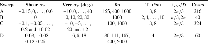
 …
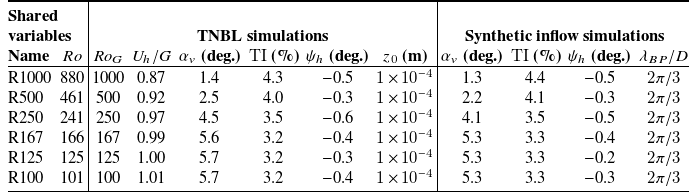
 ϕ=45∘

 a
 ⟨Δu¯⟩
 b
 Ro−1

 a
 (R500)
 b
 (R100)

 a
 (R500)
 b
 (R100)
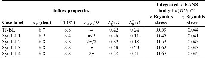
 Ro=100
 R100

 a
 b
 R100
 L0

 ϕ=45∘
 zh/D=0.625

 a
 b
 Cr
 K h−1

 a
 TI=3%
 b
 TI=8%
 c
 x0
 TI

 a
 b
 TI
 c

 a
 c
 a
 b
 c
 d
 e
 f
 y/z

 Lwake
 25%
 a
 L0y/D=0.17±0.03
 b
 R2=0.86
 c
 L0y/D=0.40±0.05

 x/D=10
 a
 c
 3%
 d
 f
 8%
 a,d
 b,e
 c,f
 ∘
 Ro=100
 ×
 Ro=1000

 αs⋅αv
 TI=3%
 x/D=10
 a
 b
 c
 e
 c
 d
 e

 x/D=10
 a
 TI=3%
 b
 TI=4%
 c
 TI=8%
 Ro−1

 10m×6.25m
 Cr=0.1,0.5K h−1

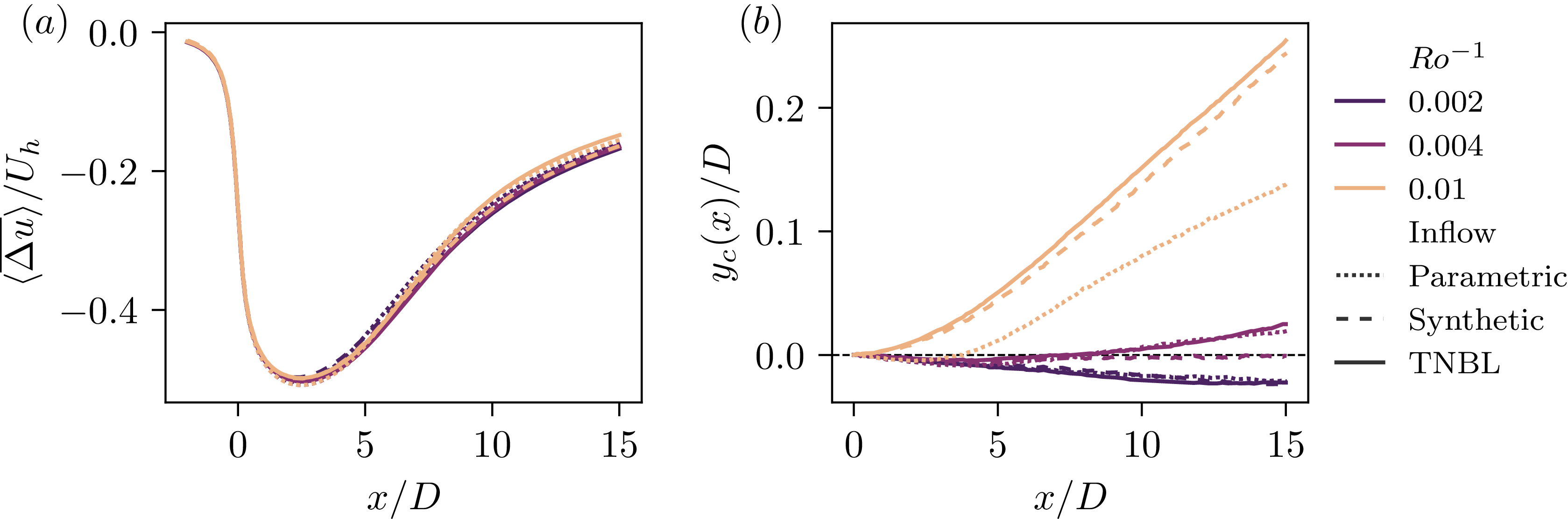

 Open access

