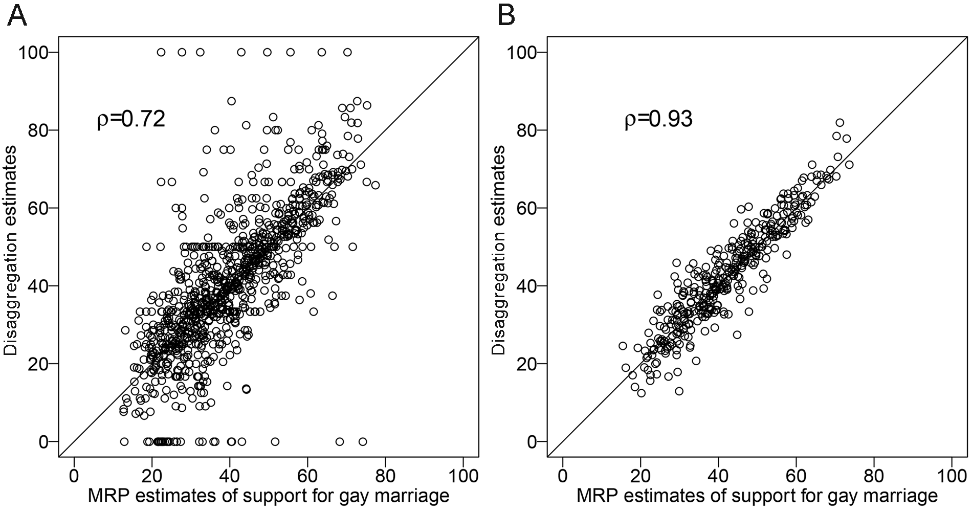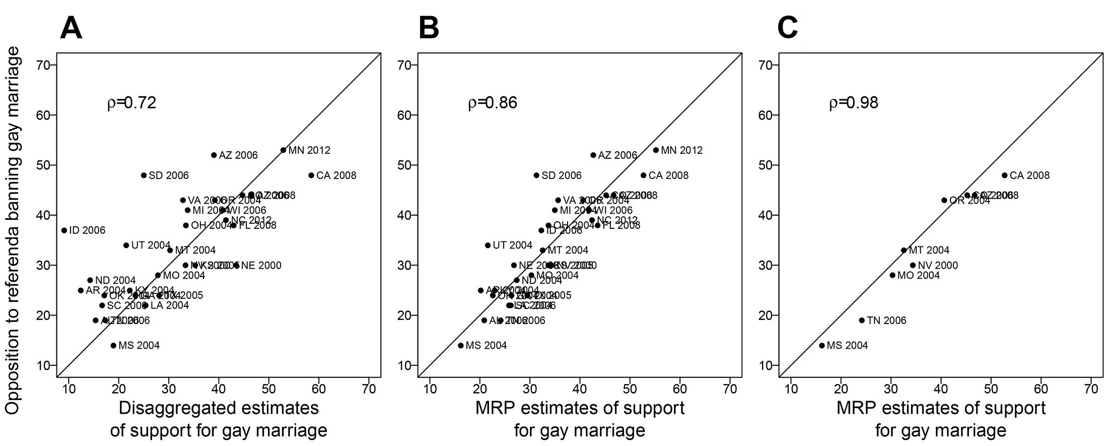


I. Introduction
Under the system of federalism in the United States, federal courts exert power over both the federal government and state governments. With their sweeping power of judicial review, federal judges can strike down federal and state laws, thereby giving federal courts the ability to affect policy implementation in all 50 states. Via their interpretation of the US Constitution, federal judges can establish a minimum level of constitutional protection that states must provide to their residents. This level constitutes a federal “floor” for legal policy, below which no state can lawfully set policy. The combination of federalism and vertical judicial review of state statutes means that the actions of federal judges and state legislatures are inherently tied together. As a result, federal courts can mediate the relationship between state policy and state-level public opinion.
In this article, I examine how the ability of federal courts to establish federal floors affects representation—specifically, the relationship between public opinion and policy at the state level. To do so, I develop a framework that is based on models of the effect of federal mandates on policy choices, when policy is a function of choices made at both the state and federal levels (Crémer and Palfrey Reference Crémer and Palfrey2000). In the framework, a federal court can unilaterally establish a federal floor in a given policy area—for example, how much protection the Constitution must provide for women to obtain an abortion without interference from states (Kastellec Reference Kastellec2018). This floor thus establishes a minimum level of protection that states must provide.
My purpose in developing this framework of judicial federalism is threefold. First, I use it to evaluate the effect of federal floors on state-level representation and thus on the development of policy in a system of federalism. Because courts can implement floors but not ceilings, the effect of judicial review of state statutes on representation is asymmetric: states in which the legislature has chosen a lower level are compelled to shift policy to the floor, while states with policy levels above the floor are unaffected. This means that the ability of policy to match the preferences of the median voter of a state will depend on the relationship between the location of those preferences and the location of the floor.
Second, I use the framework to recast the familiar “countermajoritarian difficulty”—the problem of unelected judges striking down legislation enacted by elected legislatures—as an issue of federalism. Most theoretical and empirical accounts of the countermajoritarian difficulty focus on Supreme Court invalidations of federal legislation enacted by Congress. While this use of judicial review is surely important, throughout its history the Supreme Court has been much more active in striking down state legislation than federal legislation. The framework allows for more precise definitions of when a decision is in fact countermajoritarian. Specifically, I develop versions both with and without scenarios in which the status quo at the state level may lag behind changes in public opinion, and with and without the presence of cross-state moral externalities, in which voters care about policies not just in their states but in all states. I then show that the existence of lagging status quos or cross-state externalities is a necessary condition for a decision to be classified as promajoritarian. For example, in the presence of externalities, the implementation of a federal floor benefits voters who prefer higher levels of constitutional protection, due to the positive externalities that arise from “low protection” states being forced to shift their policies. Conversely, a floor harms voters who prefer lower levels of protection, since they suffer both immediate policy losses and negative externalities from other states shifting their policies to accommodate a federal court’s mandate. Comparing net beneficiaries to net losers from the mandate allows for a classification of whether a given decision is pro- or countermajoritarian.
Finally, I use the framework to make predictions about the distribution of the types of constitutional challenges across state and federal courts. If the Supreme Court either chooses not to establish a federal floor or “lowers” the floor by reducing the amount of constitutional protections in a given issue area, the prospect of challenges being successful in lower federal courts will be minimal or reduced, owing to the nature of strict vertical stare decisis in the federal judicial hierarchy. Nonexistent or low federal floors, in turn, should induce litigants to bring more challenges in state courts, given that state court judges, via interpretation of their state constitutions, are free to raise the floor above the level of protection beyond that provided by the US Supreme Court. While this function of state courts is well known in the legal literature (Brennan Reference Brennan1977), the framework integrates this aspect of judicial federalism into a unified model of courts, legislatures, and citizens.
To illustrate the utility of the framework, I present a quantitative analysis of the path to the legalization of same-sex marriage in all 50 states, using both original and existing data on public opinion, judicial decisions, and state-level policy. Early in the debate over gay marriage, public opinion was decidedly against legalization, and federal courts provided no constitutional protections for the rights of gays and lesbians to legally marry. As a result, activists pursued challenges to state bans in state courts, some of which were receptive to these claims. As public opinion shifted dramatically in the direction of supporting gay marriage, many states implemented legalization via statutes or voter referenda. Most states did not, however, and federal courts (at every level of the federal judicial hierarchy) established a federal right to same-sex marriage over the course of 2013 to 2015. In states where opinion majorities favored retaining a ban on same-sex marriage, the implementation of a federal floor resulted in a mismatch between state opinion and policy. However, in a majority of states, federal courts actually brought policy in line with opinion majorities, due to the fact that the legal status quo lagged behind the change in public support for gay marriage. Finally, I use simulations to examine how the presence of cross-state externalities changes the effects of the introduction of federal floors on overall voter utility. These results have important implications for understanding the power of federal courts and the nature of representation in a system of federalism.
II. Federal Judicial Power, Representation, and the Countermajoritarian Difficulty
Perhaps the core tension in any federation is the division of power between the national and state governments. This tension is enhanced with respect to federal judicial power, given the ability of unelected and life-tenured federal judges to strike down both federal laws (“horizontal judicial review”) and state laws (“vertical judicial review”)—see Friedman and Delaney (Reference Friedman and Delaney2011). The ability of federal courts—particularly the Supreme Court—to exercise power over both the national and state governments has given rise to the so-called countermajoritarian difficulty. As first formulated by Bickel (Reference Bickel1962, 16–17), the difficulty is that “when the Supreme Court declares unconstitutional a legislative act or the action of an elected executive, it thwarts the will of representatives of the actual people of the here and now; it exercises control, not in behalf of the prevailing majority, but against it.” The countermajoritarian difficulty is thus fundamentally a question of representation.
The exercise of horizontal versus vertical judicial review raises distinct (if overlapping) questions about federal courts and representation. Yet quantitative evaluations of the countermajoritarian difficulty have tended to implicitly discount the importance of federalism. This can be seen in two important strands of research on the Court’s decision making. First, there exists a large literature on whether the decisions of the US Supreme Court align with majority opinion (see, e.g., McGuire and Stimson Reference McGuire and Stimson2004; Giles, Blackstone, and Vining Reference Giles, Blackstone and Vining2008). These studies tend to focus on national-level public opinion, ignoring the distribution of opinion across states. This metric makes sense when evaluating the justices’ review of federal legislation. But when the Supreme Court reviews state legislation, the metric is less clear, as the Court is potentially disrupting the connection between state-level public opinion and state policies.
Second, there is a significant literature on whether the Court is constrained by Congress or the president or both. If such constraint exists, it would potentially mitigate the countermajoritarian difficulty, since the Court would be less likely to strike down acts of Congress, which are passed by elected officials. Typically, however, these studies either focus solely on judicial review of acts of Congress (e.g., Clark Reference Clark2011; Segal, Westerland, and Lindquist Reference Segal, Westerland and Lindquist2011) or pool constitutional decisions that involve both state and federal law (Segal Reference Segal1997; Bailey and Maltzman Reference Bailey and Maltzman2008). Perhaps most famously, Robert Dahl’s (Reference Dahl1957, 282) argument that the Supreme Court only rarely will be out of step with the dominant national political coalition expressly set aside what Dahl called the “ticklish” question of the Court’s consideration of state laws (Casper Reference Casper1976).
The empirical focus on horizontal judicial review is not surprising, given the salience of the Supreme Court’s invalidation of congressional acts. Yet, this focus obscures the fact that throughout its history, the Court has been much more active in invalidating state laws than federal laws. As of 2014, according to the Congressional Research Service, the Supreme Court had directly invalidated 177 federal laws, compared to 955 state laws (Government Publishing Office 2014a, 2014b). Moreover, vertical judicial invalidations have potential implications for all 50 states. For example, in their study of the Supreme Court’s review of state statutes, Lindquist and Corley (Reference Lindquist and Corley2013, 8) find that 25% of the Court’s decisions in which it evaluates a state statute “have the potential to adversely [and directly] affect state statutes from 21 or more states,” because other states have similar or identical statutes to the one under consideration.Footnote 1 Moreover, this statistic understates the implied effect of an invalidation of a state law, since such a decision sets the floor below which no state can go, meaning the policy implications of an invalidation may extend to all 50 states. However, while their study is important, Lindquist and Corley do not evaluate the relationship among public opinion, state statutes, and the effect of the Supreme Court’s decisions.
A. The Role of Moral Externalities
How then might we frame the decision by federal courts to inject themselves into vertical politics? One way is using the lens of externalities. In the broader literature on federalism, many theories focus on economic externalities. These types of externalities—for example, how pollution in one state creates negative spillover effects in other states—are particularly salient in studies of fiscal federalism, which concern the provision of public goods across the national and state levels (Oates Reference Oates1972).
While certain types of judicial decisions—for instance, antitrust rulings—can create or mitigate economic externalities across states, decisions involving constitutional protections are more likely to implicate moral externalities (Janeba Reference Janeba2004; Cameron Reference Cameron2005). Some citizens may care not just about policy in their home state—that is, policy that directly affects them—but also policy in other states. This utility over out-of-state policy arises from moral concerns. A quintessential example in American history is slavery: Northern opposition was driven in part by disgust over the practice of slavery in Southern states, even though slavery was banned in the North (Graber Reference Graber2006). Moral externalities, of course, can run in both directions. A person opposed to abortion, for example, may suffer from abortion restrictions being minimal in other states, even if such restrictions exist in that person’s home state; conversely, a person who supports the right to an abortion and lives in a state with few restrictions may nevertheless perceive harm to women in other states with reduced access to abortions.
The presence of cross-state moral externalities means that the use of vertical judicial review may have a “unifying” function, if the distribution of preferences is such that national majorities may benefit from courts “reining in” outlier states. Whittington (Reference Whittington2007, 107) notes that “the Supreme Court has often used the power of judicial review to bring states into line with the nationally dominant constitutional vision.” Brown v. Board of Education, which struck down segregation statutes in multiple states, illustrates this function of federal courts. While there was substantial opposition to the decision, it was concentrated in the Southern states, which were directly affected; national majorities, on the other hand, favored the decision. Moreover, “northern voters were largely appalled” by many of the tactics used by officials in the Southern states to defy the Court’s decision (Klarman Reference Klarman2012, 187).
B. Courts and Status Quo Biases
A second way to frame the use of vertical judicial review is to consider the possibility that state policy may not match state majority opinion, in which case the decision by a court to alter policy may actually enhance representation. Such a disconnect may occur for several reasons. First, legislative majorities may understand the public’s desire for policy change but fear exercising such change for political reasons and thus may prefer to defer to courts and their use of judicial review (Graber Reference Graber1993; Lovell Reference Lovell2003; Lemieux and Lovell Reference Lemieux and Lovell2010). Second, the status quo biases inherent in the United States’ separation-of-powers system may actually lead to disconnect in the mapping from public opinion to policy, when the former moves and the latter does not (Lax and Phillips Reference Lax and Phillips2012; Kastellec Reference Kastellec2016). As a result, the status quo as established by statutes may lag behind public opinion, perhaps due in part to blocking by entrenched interests (Klarman Reference Klarman1997; Whittington Reference Whittington2005). As noted in Kastellec (Reference Kastellec2016, 5), “When evaluating judicial review with respect to the countermajoritarian difficulty, it is crucial to compare not just the correspondence between public opinion and judicial decisions but also how those decisions relate to the location of the legislative status quo.”
III. Judicial Federalism and Representation: A Framework
How might we incorporate the role of externalities and status quo biases into a framework for analyzing judicial federalism and representation? While not modeling the judiciary, a series of recent formal theories by Crémer and Palfrey (Reference Crémer and Palfrey1996, Reference Crémer and Palfrey1999, Reference Crémer and Palfrey2000, Reference Crémer and Palfrey2006) provide a useful foundation. Of particular relevance here, Crémer and Palfrey (Reference Crémer and Palfrey2000) present a theory that examines the effects of federal mandates—that is, a minimum policy below which no state can go—on voter utility. The establishment of a federal mandate in the first stage affects voting over state policies in the second stage, and more voters will be made worse off by the creation of a mandate than there are voters who will benefit. Cameron (Reference Cameron2005) employs Crémer and Palfrey (Reference Crémer and Palfrey2000) to develop a theory in which the Supreme Court strategically chooses whether to assert jurisdiction in a given area of the law, as a function of expected enforcement costs over states, should the Court assert jurisdiction and establish a national floor. The framework I develop builds directly off the formal theories presented in Crémer and Palfrey (Reference Crémer and Palfrey2000) and Cameron (Reference Cameron2005).Footnote 2
It is worth noting that, in developing the framework, I set aside any evaluation of whether judicial review is normatively desirable above and beyond its effect on the links between public opinion and policy. Of course, one defense of judicial review is that the Constitution prohibits some sets of policy choices—even ones that may be broadly popular—and the task of judges is to decide where that line is (e.g., Ely Reference Ely1980).Footnote 3 Alternatively, McGinnis and Somin (Reference McGinnis and Somin2004) argue that the very structure of federalism requires federal courts to intervene for citizens to best obtain the benefits of federalism. While recognizing these important normative considerations, my purpose in this article is to focus solely on the positive consequences of judicial federalism as it pertains to representation.
A. Preliminaries
I consider a federation of S states, where s denotes individual states. Each state has a continuum of voters, who are denoted by i; let i, s denote voter i in state s. It is useful to denote separate levels of aggregation within the government. Let N denote the set of all voters in all states, or the national district. Let C
1, C
2, …, Ck
denote the set of circuits within the government, of number k. The name “circuit” is derived from the US courts of appeals, which are divided into geographic units. More generally, circuits can be thought of as aggregations of two or more states. Each circuit consists of a subset of the set of all states; these subsets are both exhaustive and mutually exclusive (i.e., every state appears in one and only one circuit). Let
 generically devote a given level of aggregation.
Voters have single-peaked preferences over a one-dimensional policy space
 . Rather than a standard rendering of a one-dimensional spatial model, the policy space here is best characterized as the “amount of protection” for a specified activity by an individual. In the abortion context, for example, a policy of 0 would mean a complete ban on all abortions under any circumstances, whereas
 would mean total protection of a woman’s right to obtain an abortion under any and all circumstances. Let xs
denote the implemented policy in a given state. The policy space can encompass a wide range of issues, including issues in which ideological conservatives would prefer greater protections. For an example with reverse ideological polarity, consider the issue of gun rights; a policy of 0 would mean a complete ban on individual ownership of any firearms, while a policy of
 would mean unrestricted access to any and all firearms.
Denote the ideal point of voter i in state s as tis ; voters prefer state policies that are closer to their ideal point. For now, assume no externalities or spillovers from policies in other states. Assuming linear loss, the utility function for a voter can be stated as

It is useful to summarize the preferences of the median citizen at each level of aggregation in the government. Let ms denote the median citizen’s ideal policy in state s, mc denote the median citizen’s ideal policy in circuit c, and mn denote the “national” median voter. Let ma generically refer to the median voter at level of aggregation a.
B. The Structure of Federal Floors
In formal theories of federal mandates, state policy results from the interaction of preferences aggregated nationally as well as preferences in individual lower units (see, e.g., Crémer and Palfrey Reference Crémer and Palfrey2000). Judicial federalism and the power of judicial review simplifies matters a great deal, since courts can act unilaterally to change policy. Let FC denote a federal court, where SC denotes the Supreme Court; CC k denotes a circuit court in circuit k, and DC s denotes a district court in state s. With slight abuse of notation, denote the ideal policy of each court by this same notation. Thus, SC denotes the Supreme Court’s ideal federal floor.
In the absence of federal court action, states are unconstrained and free to choose to set policy anywhere in the policy space
 . A federal court then sets a federal floor, denoted Fa
. With Fa
in place, the set of allowable policies shifts to
 .
If implemented, Fa
applies to the jurisdiction of the court that implements it. For example, a floor set by a district court F
DC would apply only to the state in which the district court is located; a floor F
CC would apply to all the states in a given circuit; and a floor F
CC applies nationally. Under the norms of strict vertical stare decisis, federal floors set by higher courts supersede decisions by lower courts. The utility of a federal court is
 —that is, the average distance between its ideal point and all state policies that fall under the court’s jurisdiction.
C. Policy Implementation in the Absence and Presence of Federal Floors
For now, and following the basic model in Crémer and Palfrey (Reference Crémer and Palfrey2000), assume that state policy is selected via referendum. Thus, in the absence of a federal floor, state policy would be set at ms , the median voter in a state. This result follows straightforwardly from the assumptions of single-peaked preferences and a single policy dimension (and the lack of any agenda control).
Now assume that a federal court decides to implement a federal floor. Given its utility function, a federal courts’s best strategy is simply to set Fa at its ideal policy. This is because a court cannot “lower” policy in states with ideal points that are higher than FC, so it has no incentive to set the floor higher than its ideal point. Similarly, setting the floor lower makes the court weakly worse off, since states with median voters between Fa and FC will set their policies in this interval (see lemma 2 in Cameron Reference Cameron2005).
With a federal floor in place, policies below F are now off-limits, and hence state policy is set at
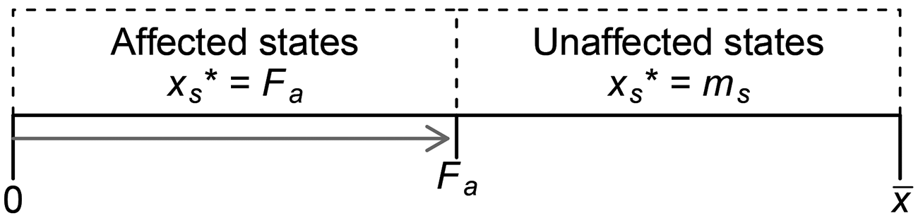
 . This result is illustrated in figure 1: all states where the median voter prefers
 see policy “shifted” to Fa
. These are the states affected by the establishment of the federal floor. Conversely, states where the median voter prefers
 are unaffected by the federal floor.
Result 1: The implementation of a federal floor only affects policies in states where the median voter is located below the federal floor. In the absence of cross-state externalities, the implementation of a federal floor also only affects voters in states where the median voter is located below the federal floor.
Effect of a federal floor on state policy making
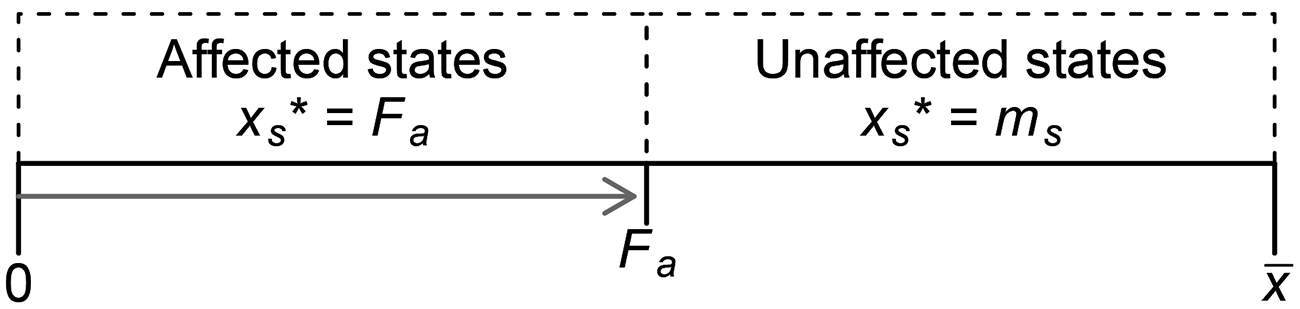
While straightforward, this result is fundamental to understanding the role of judicial review by federal courts in a federal system. The establishment of a federal floor cuts off the ability of some states—but not all states—to implement their preferred policy. In particular, those with a “low demand” for protections in a given issue are affected, while “high demanders” are not. This, of course, has important consequences for representation: it means that the ability of state policy to match state opinion when a federal floor has been set will be asymmetric.
D. Judicial Floors and Voter Utility
I now consider how the establishment of a judicial floor affects aggregate voter utility. Continue to assume that state policy perfectly matches the preferences of the median voter within each state. It is first useful to consider how the implementation of a judicial floor affects the direct policy utility of a voter within an affected state—that is, ignoring the role of any externalities. Again, the median voter in a state is the relevant benchmark: if
 , the implementation of the floor does not affect policy, and voters’ utilities are likewise unaffected. Conversely, if
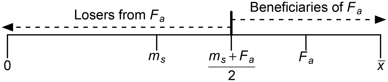
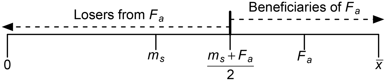
 , many voters lose from such a decision (since the floor is to the right of the median voter). Some voters, however, will benefit. Specifically, as seen in figure 2, there is a cutpoint
 that lies halfway between the median voter’s ideal point and the judicial floor. Voters to the left of the cutpoint do worse under the floor, while voters to the right do better. Not surprisingly, voters with ideal points more extreme than the median and the location of the floor have more to lose and gain, while centrist voters see smaller utility shifts. The total shift in voters’ policy utility can be expressed simply as

That is, the total shift is given by the distance between the voter and the median state voter (i.e., the “old” policy), minus the distance between the voter and the new policy, which is determined by whether the voter’s state is affected by the federal floor. By construction, γ s cannot be positive: setting the floor at or below the state median voter does not affect voters’ policy utility, while setting it above induces an overall decline in utility.
Winning and losing voters
When we move to federal decisions that affect multiple states (i.e., circuit courts or the Supreme Court), the effect of judicial floors on aggregate voter utility is subtler. The calculation of net shift in voters’ policy utility proceeds similarly, only now we consider all voters in level a:

The location of the state median voter is still the benchmark, but now the relevant comparison is a judicial floor that affects voters in multiple states. It is straightforward to see that γ a also cannot be positive: the floor does not affect voters in states with median voters above the floor, but it induces a shift in policy away from the ideal point of voters who reside in states with median voters below the floor.
For illustration, consider the following numerical example. Suppose there are three states comprising a total of 99 voters, with 22 voters in state 1, 45 in state 2, and 32 in state 3. Let
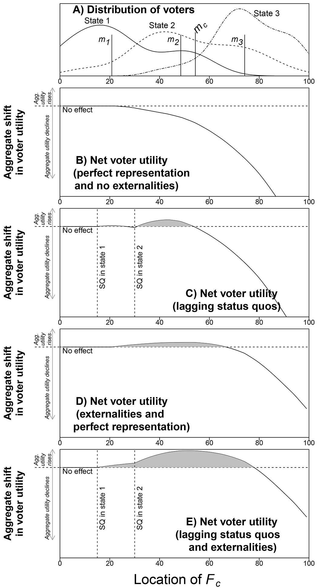
 . In each state, the ideal points of voters are drawn from a normal distribution; the mean ideal point of voters is increasing in each state. Specifically, the mean ideal point is 25, 50, and 75 in states 1, 2, and 3, respectively, with a standard deviation of 20 in each state (ideal points below 0 and above 100 are truncated at the limits). Figure 3A
depicts these distributions, along with the location of the respective median voters in each state.
Effect of a federal floor. A, Distribution of voters in a hypothetical three-state example. B–E, Aggregate shifts in utility as the floor is set sequentially from 0 to 100, under the scenarios described in each panel label. See text for further details.
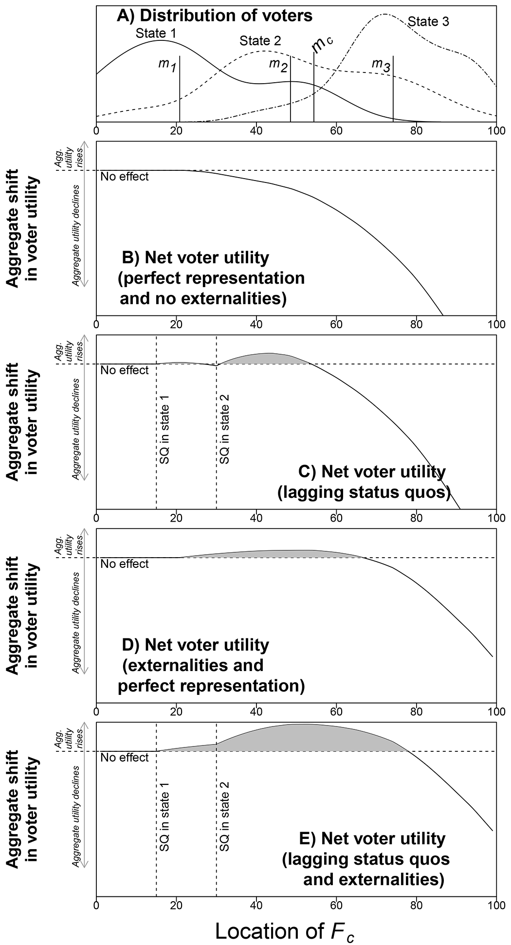
Suppose these three states are in the same circuit—mc
depicts the overall circuit median—and a circuit court sets a floor Fc
. Imagine the floor was set sequentially at every integer on x—figure 3B
depicts the net utility shift from setting the floor at a given location on the horizontal axis. The dashed horizontal line indicates a net utility shift of zero—values above and below this line respectively indicate positive and negative shifts in voter utility, by comparing net voter utility before and after the introduction of a federal floor at each specific value. Figure 3B
shows that there is no effect of establishing a federal floor until it hits just above the location of m
1 (around 20), at which point the extreme low-demand voters in state 1 suffer a utility loss from the floor being set above m
1. As the floor gets increasingly higher—particularly when it exceeds m
2 and m
3—more voters are increasingly affected. As the floor approaches
 , only the most high-demand voters benefit, while all other voters suffer a utility decline.
E. Incorporating State Legislatures and Status Quo Policies
So far I have assumed that state policy is set via referendum. Thus, in the absence of judicial intervention, state policy would be set perfectly at the location of the state median voter. Now assume that state policy is decided by a representative legislature. One possibility is that legislatures perfectly reflect the will of state majorities. In Crémer and Palfrey (Reference Crémer and Palfrey2000), shifting from a referendum system to elected legislatures has a substantive impact on policy, as it results in the federal mandate being placed at the median of all median voters across districts, rather than the overall median of all voters. In the model here, however, it actually produces no meaningful differences, given that Fa
is set by a court. If state legislatures perfectly represented the state median voter, then state legislatures would set policy at
 , and everything would be the same as above.
Now consider the scenario in which this is a potential mismatch between state policy and current state-level opinion. Let qs
denote the status quo policy of state s. Accordingly,
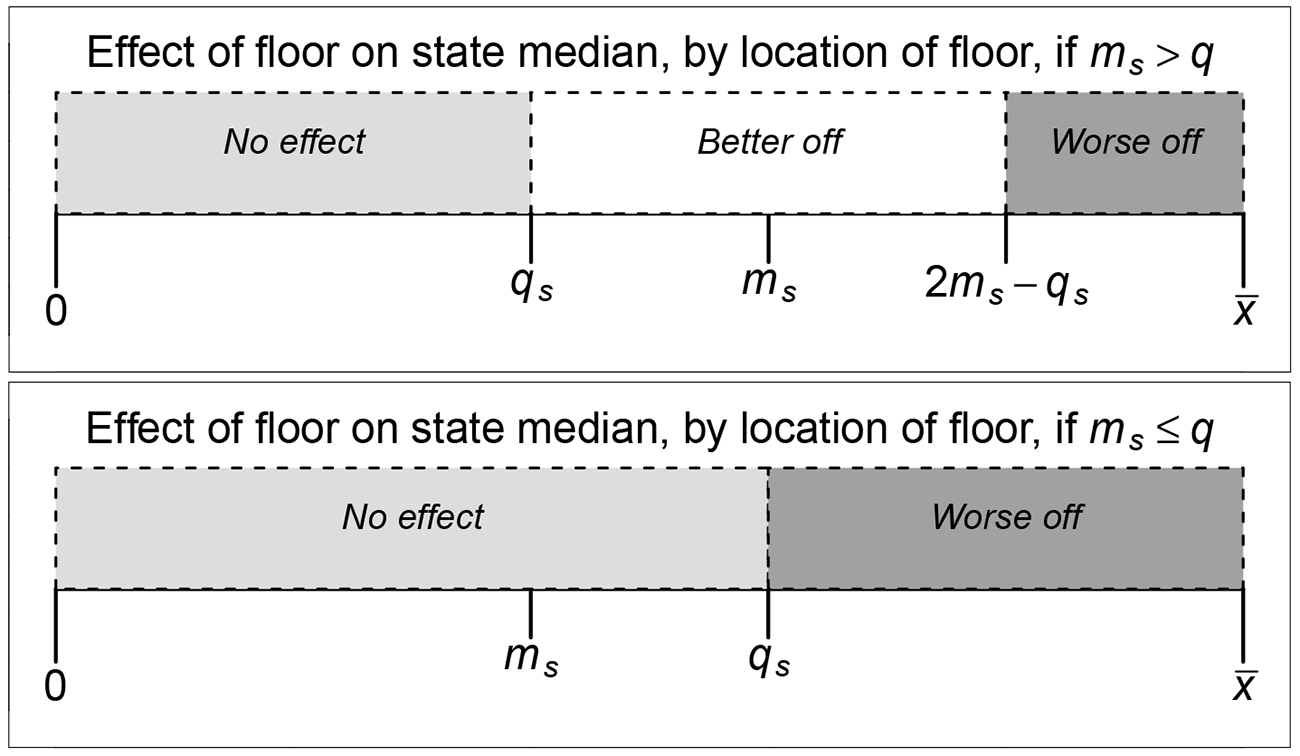
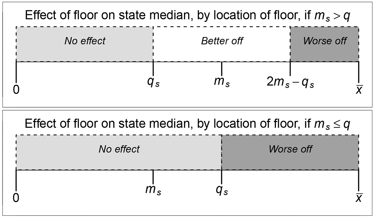
 represents the lag between what the current state median prefers and existing policy. Thus, there exists a range of federal floors that will improve upon the utility of the median voter; whether this is the case depends on the location of the state median relative to the status quo. Specifically, if
 , any floor that is to the right of qs
and to the left of
 will benefit the median voter. Conversely, if
 , then the introduction or movement of a federal floor either has no effect or makes the state median voter worse off: the former occurs if
 , the latter, if the floor is above qs
. Again, we see the asymmetric effect of federal floors, which is visualized in figure 4: they only improve the representation of voters who are “higher” on a given policy dimension.
Effect of a federal floor on state median utility, depending on whether the median is to the right of the state status quo (top) or the left of the status quo (bottom).
Returning to the question of how federal floors affect aggregate voter utility, we can restate equation (3) but with qs replacing ms :

To see how the inclusion of lagging status quos may affect representation, I return to the numerical example in figure 3. Whereas previously state policy defaulted to the location of the state median voter, now assume that the status quo in states 1 and 2 lags “below” the location of the median: specifically, assume
 and
 (
 and
 ). Figure 3C
presents the shift in net voter utility, at every level of the federal floor. Because many more voters in states 1 and 2 benefit from even floors well above their ideal point (in contrast to what we saw in fig. 3B
), there are now regions (indicated via shading) in which the establishment of a federal floor increases voter utility—particularly in the region between
 and just above ms
2; floors in this range benefit many voters in state 2 (and state 1 as well) while not affecting voters in state 3.Footnote
4
F. Adding Externalities
Now let us introduce the possibility of cross-state externalities in voters’ utility functions. To motivate this possibility, I modify the voters’ utility function as follows:

where
 denotes the sensitivity of voter (i, s) to policy in states
 , and
 denotes the relative size of state s, with
 . Thus, externalities for an individual voter are weighted by the distance between her ideal and policy in all other states, as well as the relative size of each state.
Given this utility function, the total shift in voter’s utility after the introduction of a federal floor can be expressed as follows:

While this expression is more complicated, the basic intuition is the same: voters compare their utility under the absence of a federal floor to that under the floor, which will now affect their utility gained or lost from policies being moved in states affected by the floor, even if their state is unaffected directly by the introduction of a floor.
How does the introduction of externalities affect the overall picture of voter gains and losses? Returning to the numerical example, figure 3D depicts the shift in aggregate voter utility as the federal floor is set increasingly higher. To highlight the importance of externalities, figure 3D returns to the assumption of perfect representation (i.e., state policy is set at the location of the median state voter), as assumed in figure 3B . For simplicity, I assume that α is is uniformly distributed between 0 and 1 and that ɸ j is based directly on the number of simulated voters in each state.
Figure 3D shows that the introduction of “moderate” floors—here in the range of roughly 25–70—induces positive net voter utility shifts (again indicated by the shaded region). This is because even though the setting of a floor has no in-state direct effect on many voters’ policy utility, high-demand voters now reap the gains from low-demand states being forced to set higher policies, thereby moving out-of-state policy closer to the high demanders’ ideal points. This shift, of course, induces negative externalities for low-demand voters (these externalities are on top of their in-state policy loss). However, in this example, only when the floor exceeds 70 or so (i.e., above m 3) do the overall utility losses from the floor exceed the benefits. This example illustrates the classic case of courts bringing “outlying minorities” in line with national majorities, as voters who favor higher protection see federal courts move policy closer to their ideal points in states where the median voter prefers lower levels of protection.
What happens if we allow for both lagging status quos and the presence of cross-state externalities? Figure 3E combines the analyses in figures 3C and 3D . That is, the status quos lag behind the median voters in both state 1 and state 2, and the same distribution of externalities analyzed in figure 3D is assumed. Figure 3E reveals that, in this scenario, utility gains exist from the setting of federal floors at every level except very low levels (where they have no effect) and very high levels (beyond the ideal point of the median voter in state 3).
G. Defining a Countermajoritarian Decision
Taking the analyses of federal floors as a whole, the judicial federalism framework directly facilitates a definition of whether a decision is countermajoritarian. We can simply look at the effect of an introduction of a federal floor and evaluate its effect on overall voter utility. Recall that by construction, γ
s
cannot be positive; this means that when only direct policy utility is considered, and if perfect representation of the median voter is assumed, a federal court decision to establish a floor must be countermajoritarian (as long as the floor affects at least one state). However, allowing for lagging status quos or externalities changes things, as both
 and
 can be positive. If they are positive, then more voters are benefiting from the court’s setting of a federal floor—such a decision is thus promajoritarian. If
 or
 is negative, however, then the decision is countermajoritarian. This leads directly to this result:
Result 2: A necessary condition for the establishment of a federal floor to be promajoritarian is either the existence of lagging status quos or the presence of cross-state externalities.
One upshot of this result is that it is not straightforward to evaluate whether a decision by a federal court is pro- or countermajoritarian. Such determinations must be made in light of both the location of the status quo in each state and one’s assumptions about how voters evaluate out-of-state policy.
H. State Courts
In this section, I introduce state courts, which comprise the final piece of the judicial federalism framework. Under the supremacy clause of the US Constitution, state courts are obligated to respect floors set by the Supreme Court, but they can also interpret their own state constitutions as providing greater protection (Devins Reference Devins2010). Let SF
s
denote a floor set by a state court in state s, where
 .Footnote
5
If a state court sets a floor, then policy is set at
 .
This aspect of the model speaks directly to the so-called new judicial federalism (see, e.g., Devins Reference Devins2010). As the Burger and Rehnquist courts turned rightward and limited the Supreme Court’s interpretations of individual rights, liberals turned to state courts for judicial expansion of such rights. In essence, they were asking state courts to set constitutional floors far above the level the US Supreme Court was willing to extend.
One implication of the fact that state floors can be above but not below the federal floor is that state courts should be more active in areas of the law with lower federal floors, since litigants are less likely to bring those cases to federal courts. Even when the Supreme Court has ruled a restriction constitutional, based on the justices’ understanding of the federal Constitution, state judges may still find it unconstitutional under their state constitution.
IV. Evaluating the Legalization of Gay Marriage
To illustrate the judicial federalism framework, I turn to a quantitative analysis of the legalization of gay marriage. The point of this analysis is not to engage in hypothesis testing but rather to illustrate how the judicial federalism framework helps us understand the extent to which the implementation of same-sex marriage by courts was, in fact, countermajoritarian. In particular, I demonstrate how the presence of lagging status quos and cross-state moral externalities can change one’s assessment of this question. Finally, I show that the existence of externalities has a “multiplier” effect that intensifies the extent to which the introduction of a federal floor is either counter- or promajoritarian, depending on the distribution of public opinion when the floor is introduced.
The issue of same-sex marriage is particularly well suited for applying the judicial federalism framework, for several reasons. First, there has been significant variation both over time and across states in public opinion. Second, in a majority of states, legalization was implemented by courts, with state courts, lower federal courts, and the US Supreme Court all playing a role in striking down existing state bans on gay marriage. Third, as I discuss below, the issue of cross-state externalities has played a significant role in both public opinion on the issue and judicial deliberations regarding the proper role of the judiciary in bringing about this particular social change. Finally, the battle over gay marriage nicely captures the complexities of policy change in a system of federalism; as Keck (Reference Keck2009, 156) notes, since the 1990s, “the legal and political conflicts over [gay] rights have been highly decentralized, with multiple simultaneous battles proceeding in various state judiciaries, 12 federal circuits, and at times the Supreme Court, the White House and the governors’ mansions, the halls of Congress and the state legislatures, and in about half the states, the direct democracy process as well.”Footnote 6
The history of same-sex-marriage reform—which came about in the larger context of the broader liberalization of gay rights—has been well documented, and only a brief review is necessary here.Footnote 7 Same-sex marriage first emerged as an issue in the early 1970s, with courts rejecting the first claims of a constitutional right to gay marriage. The first explicit state legislative bans were passed in that decade, although only in a handful of states.
The debate moved to the national stage in the early 1990s, sparked by a decision of the Hawaii Supreme Court (Baehr v. Lewin, 852 P.2d 44). The court did not directly rule on the constitutionality of gay marriage in Hawaii but expressed deep skepticism that the refusal of state officials to provide wedding licenses to same-sex couples satisfied the state constitution’s guarantees of equal protection. This decision sparked a huge backlash, both in Hawaii and nationally. Many state legislatures moved swiftly to pass bans on gay marriage, while in 1996 Congress passed and President Clinton signed the Defense of Marriage Act (DOMA), which both permitted states to refuse to recognize same-sex marriages from other states and prohibited the federal government from recognizing same-sex marriages for the purposes of federal law. Over the next decade or so, voters in a majority of states would pass constitutional amendments to their state constitutions expressly banning same-sex marriage.
Even against this backdrop, many state courts became more receptive to arguments against the constitutionality of same-sex-marriage bans. In 1999, for example, Vermont’s supreme court ordered the legislature to either allow same-sex marriage or implement civil unions (with equivalent benefits to marriage; Baker v. State of Vermont, 744 A.2d 864); the legislature chose the latter in 2000. In 2004, Massachusetts became the first state to legalize, following a ruling a year earlier by the Massachusetts Supreme Court that the state constitution precluded a ban on same-sex marriage (Goodridge v. Department of Public Health, 798 N.E.2d 941). In this period, public opinion began to move toward favoring gay marriage. Direct causality (and its direction) is difficult to infer, but it seems likely that state courts both took changing public opinion into account and also (in some states, at least) helped shape public opinion (Hume Reference Hume2013).
A few years later, supporters of gay marriage brought several challenges in federal court to DOMA, which the US Supreme Court struck down (in relevant part) in 2013 (United States v. Windsor, 133 S. Ct. 2675). The majority opinion, however, expressly declined to rule on the constitutionality of state bans on same-sex marriage. Over the next two years, numerous challenges to individual state bans were brought in federal courts, with many (although not all) federal district and circuit judges voting to strike bans as unconstitutional. (Over this period, many states had legalized same-sex marriage via either legislation or ballot initiatives.) Finally, in 2015, the US Supreme Court found a constitutional right to same-sex marriage, making it legal in all 50 states (Obergefell v. Hodges, 135 S. Ct. 2584).
To place this history within the confines of the judicial federalism framework, first note that the fight over gay marriage (and gay rights more generally) maps neatly into the policy space considered in the model. The dimension represents the amount of protection gay individuals have against state preclusion of the benefits of marriage. Preferences higher on the dimension indicate greater support for the rights of gay Americans; a policy of 0, for example, would mean the complete denial of any such benefits, whereas
 denotes the full panoply of marriage rights and the name of “marriage.” Thus, the federal floor for the protection of same-sex marriage is now at its maximal level. Civil unions, which some states implemented before the legalization of gay marriage, represent an intermediate policy between complete bans and complete allowance.
A. Data
To evaluate the links among public opinion, judicial decisions, and state policy, I collected data on all three.Footnote 8 (Complete details on the data collection components can be found in the appendix.) First, using multilevel regression and poststratification (MRP), I generated dynamic estimates of state-level opinion on whether gay marriage should be legalized, for each year between 1993 and 2015.Footnote 9 To capture changes in opinion over time, as well as cross-state heterogeneity, I used a model that estimates varying intercepts for states, in which these intercepts are allowed to vary over time. These estimates were created in a fully Bayesian manner. I summarize public opinion using the median estimates from the relevant parameters; also, whenever possible, I incorporate the uncertainty of the estimates (based on their posterior distribution).Footnote 10
Next, for each year from 1993 to 2015, I measured both when and how states implemented bans on gay marriage (either statutorily through state legislation or via amendments to state constitutions).Footnote 11 I then measured when each state legalized gay marriage and whether it was done via legislation (or referenda) or via judicial decisions. For the latter, I collected a data set of state and federal decisions that ruled on the constitutionality of state gay-marriage bans. For state decisions, I collected only those decided by state supreme courts. For federal decisions, I collected the universe of decisions by district and circuit court judges.
B. Initial Public Opinion and State Policy
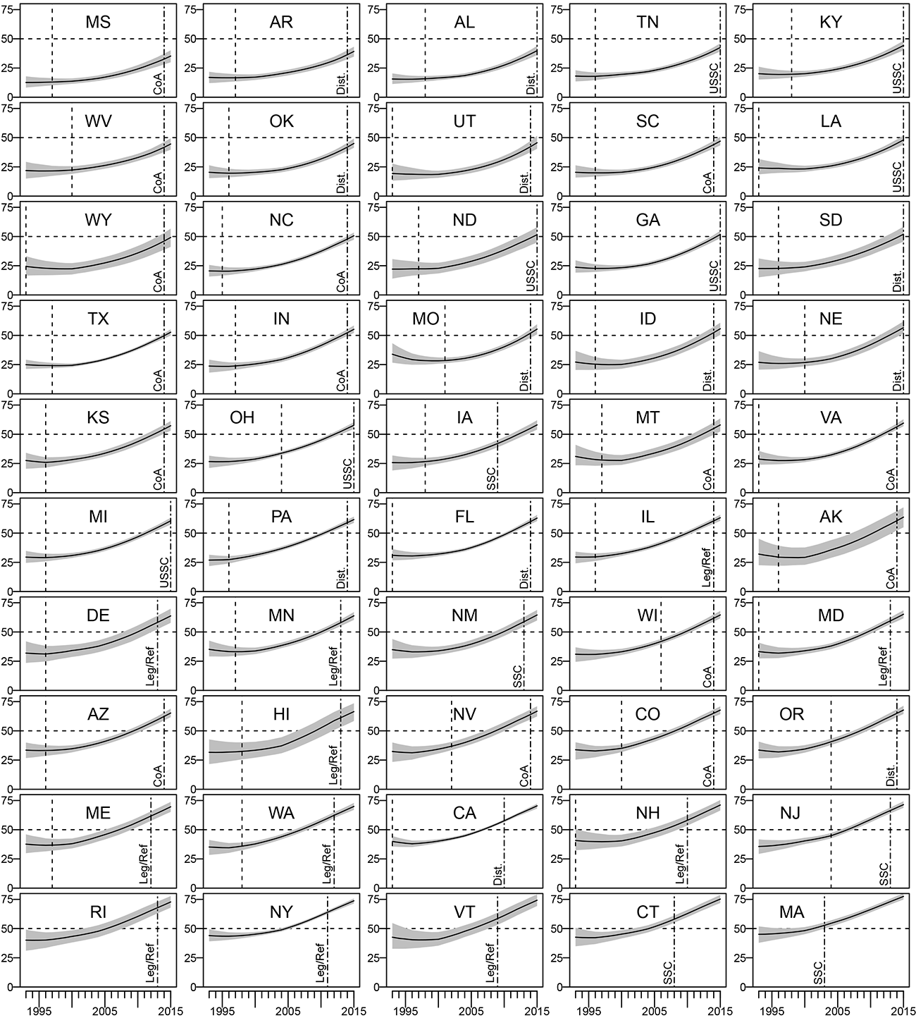
Figure 5 depicts the estimates of public opinion in each state from 1993 to 2015; the shaded regions depict 95% confidence intervals. In each plot, the vertical axis depicts the estimated percentage of residents in each state who support legalized gay marriage. The states are sorted from lowest to highest support, on the basis of the 2015 estimates of opinion. In line with the trend in national support, the figure shows an increase in support in every state over this period. However, both the base rate of support (i.e., the intercept) and the slope of change differ significantly across states. At the low end, for example, support in Mississippi rose from 13% (95% confidence interval of [8%,18%]) in 1993 to 35% [30%,40%] in 2015. At the high end, support in Massachusetts started at 45% [38%,52%] and rose to 77% [75%,80%]. Early in this period, however, public opinion was decidedly against gay marriage, even among the states that would eventually come to support it. The earliest estimated support for gay marriage to cross 50% in any state was in 2002 (in Massachusetts); the median year across states for crossing the 50% threshold (including states still below it as of 2015) was 2012.
State-level support for gay marriage, 1993–2015. States ordered by increasing support as of 2015. Dashed lines indicate when bans were passed (before 1993 depicted at 1993). Dot-dashed lines indicate when and how gay marriage was legalized. Leg/Ref = via legislation or referenda. SSC = state supreme courts. Dist. = federal district court. CoA = federal courts of appeals. USSC = US Supreme Court.

Next, the dashed lines in figure 5 depict the year in which a state first implemented a ban on gay marriage, through either statutory or constitutional means. (The dot-dashed lines depict the year and method by which gay marriage was legalized; I return to this below.) The earliest ban was enacted in 1973. (Eight states implemented bans before 1993; for convenience in fig. 5 I indicate their passage year at 1993.) The latest year of initial implementation was in 2006. Figure 5 shows that for every state that implemented a ban, public opinion at that time opposed legalized gay marriage, and thus these bans matched public policy with majority opinion—this can be seen by examining the intersection of the opinion estimates with the dashed lines, which always occurs below the 50% level of opinion.Footnote 12 Thus, the only mismatches in representation occurred in the small number of states that did not pass bans on gay marriage. However, as discussed in footnote 11, even in these states same-sex couples did not enjoy equivalent marriage rights to opposite-sex couples, and thus policy in effect matched public opinion.
If public support for gay marriage had remained at the low levels seen in the 1990s, the implementation of a federal floor (or a state court striking down gay marriage) would have been highly countermajoritarian, given that a majority of voters in no states supported it. Indeed, this fact helps explain the extensive backlash to the Hawaii Supreme Court’s decision in 1993 and the fear that courts would impose same-sex marriage on the country. In terms of figure 1, such an imposition would mean that every state (in the relevant jurisdiction) would be affected by the federal floor. However, public opinion on gay marriage shifted rapidly in the 2 decades that followed, leading voters, legislators, and courts to respond in different ways.
C. Low Federal Floors and State Court Rulings
In this section, I evaluate the role of state courts in adjudicating challenges to existing bans on gay marriage. Recall that a consequence of a low (or nonexistent) federal floor is that litigants should be more likely to bring challenges in state courts. In line with the overall trajectory of the issue over the past 3 decades, the US Supreme Court initially established a very low level of protection for gay rights. In 1972, the Court dismissed an appeal of a decision by the Minnesota Supreme Court that upheld the denial of a marriage license to a same-sex couple (Baker v. Nelson, 409 U.S. 810). In 1986, the Court upheld the constitutionality of state bans on sodomy (Bowers v. Hardwick, 478 U.S. 186); this precedent led lower federal courts in subsequent years to reject challenges to other forms of discrimination against gays, such as employment discrimination (Klarman Reference Klarman2012, 38). Ten years after Bowers, the Court issued its first decision in support of gay rights, striking down a Colorado constitutional amendment that prohibited any type of government action intended to protect gay persons against discrimination (Romer v. Evans, 517 U.S. 620). Then, in 2003, the court overruled Bowers but did not address the constitutionality of same-sex-marriage bans (Lawrence v. Texas, 539 U.S. 558).
As a result, until very recently, litigants and interest groups seeking to challenge gay marriage bans had little reason to believe that federal courts would be receptive to their claims. Thus, early efforts focused on state courts in more liberal states (such as Hawaii, Alaska, Vermont, and Massachusetts) where judges might be more receptive to striking down bans based on their state constitutions (Klarman Reference Klarman2012, 55, 89).
Public reaction to these decisions was not monolithic. For example, unlike in Hawaii and Alaska, there was little backlash against the Vermont Supreme Court’s 1999 decision mandating that the state provide same-sex couples the same rights and benefits as married couples (Hume Reference Hume2013, 75). Nevertheless, these early decisions (particularly the 2003 Massachusetts decision) in support of gay marriage rights, combined with the Supreme Court’s decision in Lawrence v. Texas in 2003, helped spur a movement among gay marriage opponents to push for amendments to state constitutions banning same-sex marriage. Such bans had been passed in 4 states before 2003; in 2004 alone, voters in 13 states approved referenda banning same-sex marriage, and by 2012, 31 states would amend their constitutions. These amendments effectively made state courts off-limits to challenges seeking legalization in those states. In the terms of the model, these amendments meant that state supreme courts could not interpret their constitutions as providing protections above the federal floor (which at the time was also 0), since the amendments explicitly ruled out such interpretations.
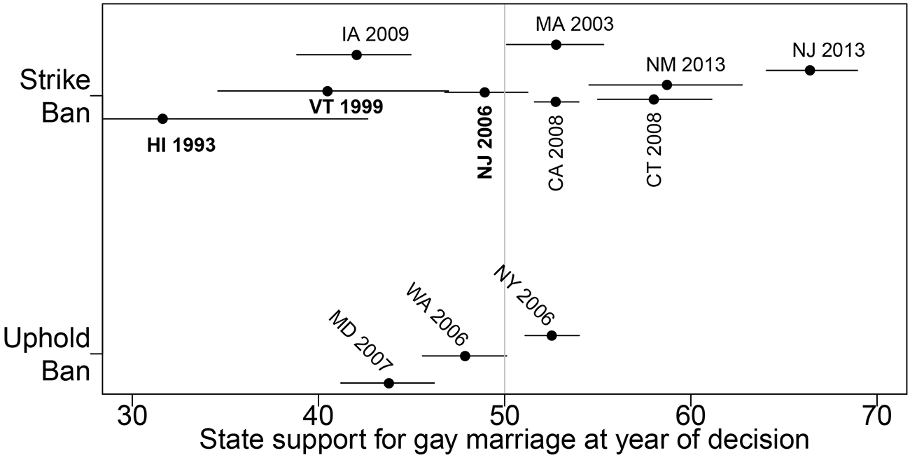
As a result, state supreme courts only heard challenges in a subset of the states that did not implement such constitutional bans. Unsurprisingly, public opinion was relatively liberal in these states. Figure 6 depicts the states in which state supreme courts ruled on gay marriage bans. The points (which are jittered vertically) depict the level of public opinion in that state in the year (indicated by the state-year label) in which a decision was issued; the horizontal lines indicate 95% confidence intervals. Decisions in which the court upheld (struck down) the ban are on the bottom (top) of the graph; the boldfaced labels indicate decisions in which the Court did not fully mandate the legalization of same-sex marriage, instead requiring the state to implement the functional equivalent (i.e., civil unions).
State supreme court decisions on gay marriage bans. The points depict estimated state-level support, in the year a court issued a given decision, with 95% confidence intervals indicated by the horizontal lines. Decisions in which the court upheld (struck down) the ban are on the bottom (top) of the graph. Boldfaced labels indicate decisions in which courts did not fully mandate the legalization of same-sex marriage but required the state to implement the functional equivalent (i.e., civil unions).
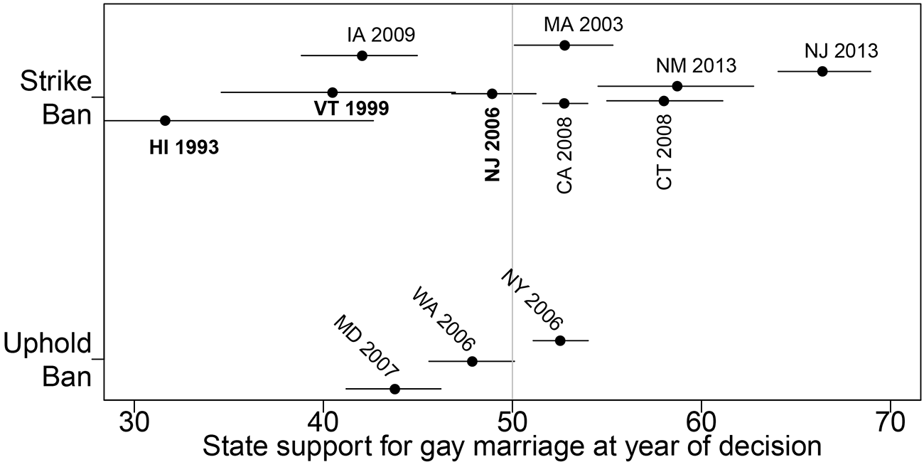
How well did the decisions of state judges align with state-level public opinion? A total of 11 challenges were heard in 10 states (the New Jersey Supreme Court heard challenges in both 2006 and 2013). As figure 6 shows, in all but 3 states in which supreme court judges either struck down state bans on gay marriage or mandated the functional equivalent of marriage (i.e., civil unions), public support for legalization was either close to 50% or well above it. As noted earlier, the Hawaii Supreme Court’s 1993 decision was highly unpopular, with just 32% [21%,44%] favoring same-sex marriage at the time. While less countermajoritarian, the Vermont Supreme Court’s 1999 decision placed the court ahead of public opinion. Finally, only an estimated 42% [38%,45%] supported gay marriage in Iowa when its supreme court legalized gay marriage in 2009.Footnote 13 Conversely, state judges in Maryland, Washington, and New York rejected challenges. Thus, while state judges in only a relatively small number of states interpreted their constitutions as providing protections above the federal floor in this period, in these states the judges were usually aligned with public opinion.Footnote 14
D. The Introduction of Federal Floors: Changing Public Opinion and Lagging Status Quos
While the first federal challenge to a state ban on gay marriage was heard in 2005 (excluding the case of Baker v. Nelson in 1971), it was not until after the US Supreme Court decided Windsor in 2013 that challenges reached federal courts in large numbers. The 16 states in which legislators, voters, or state judges had implemented same-sex marriage would, of course, be unaffected by the introduction of a floor, since policy was already above it. All told, federal courts heard 44 challenges to policies in these 34 states; the overlap is due to challenges for a particular state being heard by both the district court and the court of appeals (and, in one case, also at the US Supreme Court). Thirty-six of these decisions resulted in invalidations of state bans, while eight decisions upheld them as constitutional.
How can we evaluate how federal decisions affected all other states in light of the theory of judicial federalism? First, setting aside for now any cross-state externalities, we can ask how countermajoritarian was each decision. As shown in figure 3B, if state policy perfectly matched the preferences of the state median voters, then the introduction of a federal floor would necessarily be countermajoritarian (even as voters “above” the median in states with bans would benefit). The existence of lagging status quos, however, means that federal floors can be welfare improving in some states.
How prevalent were such lagging status quos? Even as voters in many states approved constitutional bans on gay marriage in the middle of the 2000s, public opinion was swiftly moving in the direction of support for legalization. At the same time, the passing of such bans not only prevented state courts from interpreting their state constitutions, but they also helped to make this status quo more difficult to change in many states, as doing so would require a constitutional amendment and not regular legislation (i.e., a statutory change). Thus, in many states, the shift in public opinion created the “lagging status quo” scenario seen at the top of figure 4.
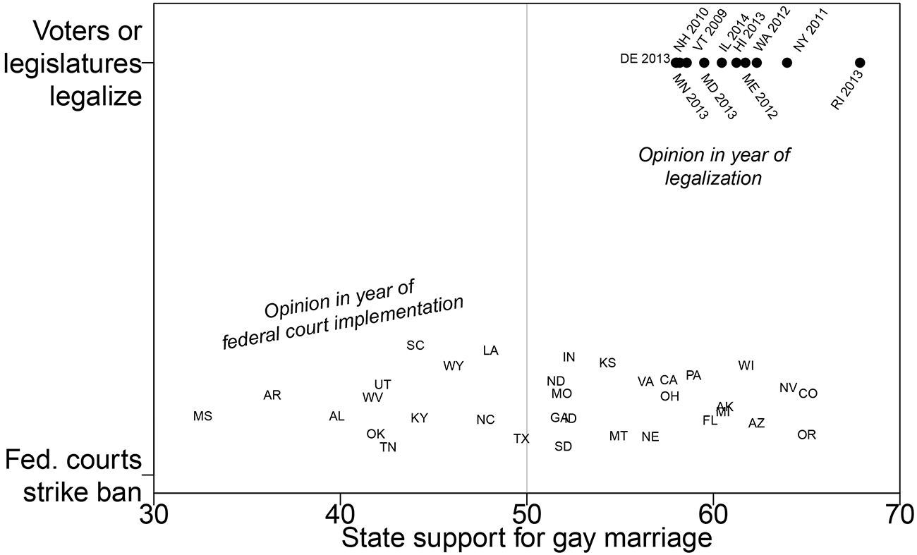
Figure 7 illustrates the relationship between public opinion and the status quo. The horizontal axis depicts estimated state-level support. The vertical axis distinguishes states where voters or legislators legalized gay marriage (this occurred in 11 states) from states where bans were kept in place—until they were eventually struck down by a federal court. Beginning with the top of the graph, the points and labels give the level of opinion in the year in which each state implemented legal gay marriage. (For example, the Vermont legislature approved same-sex legislation in 2009, at which point an estimated 59% [53%,63%] of state residents favored it.) Recall from figure 5 that in every state a majority of residents did not support gay marriage early on; however, figure 7 shows that by the time of legislative or voter implementation, public support was well above 50%. Thus, in these states, policy was shifted to match the preferences of the state median voter as those preferences moved away from the status quo; in terms of figure 4, qs and ms became aligned again.Footnote 15
State support for gay marriage versus decisions by voters/legislators to legalize, versus implementations by federal courts. See text for details.
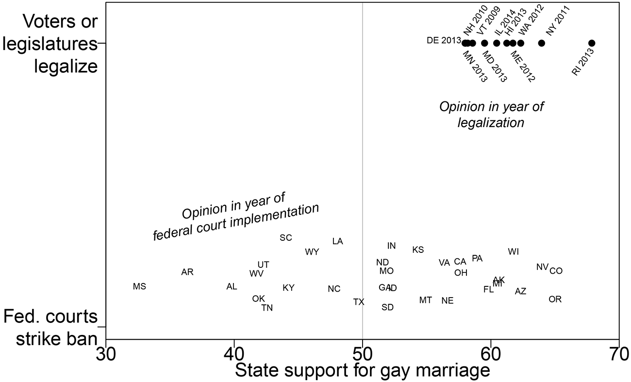
Next consider the bottom of figure 7, which depicts states that maintained their bans (until federal courts struck them down); states in which state courts implemented same-sex marriage are not included. The state labels indicate the levels of estimated opinion in the year federal courts acted (the height of the labels are jittered to make them easier to read); the first federal judicial invalidation of a state ban came in 2010 (California), while the last came when the US Supreme Court decided Obergefell in 2015.Footnote 16 Comparing the top and bottom of the figure, it is clear that the states where federal courts eventually struck down bans are ones that tended to have lower support for gay marriage. However, in many states, existing policy lagged behind the movement in public opinion. At the time of federal judicial intervention, fully 21 states had opinion majorities in favor of same-sex marriage where bans nevertheless remained in place. While support in some of these states (e.g., Georgia and Missouri) was only just above 50%, in states like Colorado, Oregon, and Nevada, sizable majorities in favor of same-sex marriage existed. Thus, the judicial implementation of gay marriage in these states was promajoritarian, as these decisions removed the lag in the status quo and brought policy in line with public opinion.
E. The Role of Cross-State Externalities
To this point, the analysis has set aside the possibility of cross-state externalities and how they might affect the relationship between public opinion, state policy, and federal floors. However, as is the case with many hotly contested social issues, the issue of moral externalities has been front and center in the fight over gay marriage. This has been particularly true with respect to opponents of same-sex marriage, many of whose arguments have focused on the deleterious effect that legalization might have on broader societal norms (Hatzis Reference Hatzis2006). Allen and Price (Reference Allen and Price2015, 146) summarize these arguments (without necessarily endorsing them) as follows:
A legal change that recognizes same-sex couples as “married” could change the cultural and social meaning of marriage for everyone, and therefore change both well-being and behavior. It has been argued, for example, that same-sex marriage accentuates the view that marriage is based on love, not children and commitment. When such a view is generally adopted it can have effects on marital behavior in general. Persons in loving relationships might be quicker to marry, and married persons who come to consider their relationship to be unloving might be more willing to divorce. Hence, marriage and divorce rates might change through this general change in social norms, which could result from same-sex marriage.
Such beliefs help explain the extent of the backlash to the Hawaii Supreme Court’s decision in the 1990s. On the one hand, the scope of the backlash is surprising, given that the strength of public opposition to gay marriage at the time made it unlikely that legislators or judges in other states would follow suit. On the other hand, if opponents of gay marriage suffered negative externalities from the potential implementation of gay marriage in even a single state, the reaction makes more sense.Footnote 17
In addition, in this period, the issue of gay marriage was likely less salient among some supporters of gay marriage, relative to opponents. Posner (Reference Posner2003, 36), for example, argued that “it is apparent from [the state of the law and public opinion at the time] that the opponents of homosexual marriage feel much more strongly about the issue than the supporters … [and] are passionate in their opposition because they feel deeply threatened by the proposed change in the concept of marriage.” Accordingly, the implementation of a federal floor in 2003 would have likely induced significant negative externalities for opponents of gay marriage that would have outweighed positive externalities for supporters. However, as opinion has evolved toward greater support for gay marriage, it seems likely that the sensitivity of supporters to out-of-state policies has grown concomitantly. One reason is that more Americans now report having family members or friends who are gay (Pew Research Center 2015).
How, then, should externalities factor into the analysis of the introduction of federal floors for gay marriage? First, as discussed in Section II.B, one way to place the issue of cross-state externalities within debates over the countermajoritarian dilemma is to think about the Supreme Court specifically (and federal courts more generally) “using the power of judicial review to bring states in line with the nationally dominant constitutional vision” (Whittington Reference Whittington2007, 107). While it would be overreaching to say that a “dominant constitutional vision” had emerged by the time federal courts started striking down state laws, a clear national majority in favor of same-sex marriage was in place.
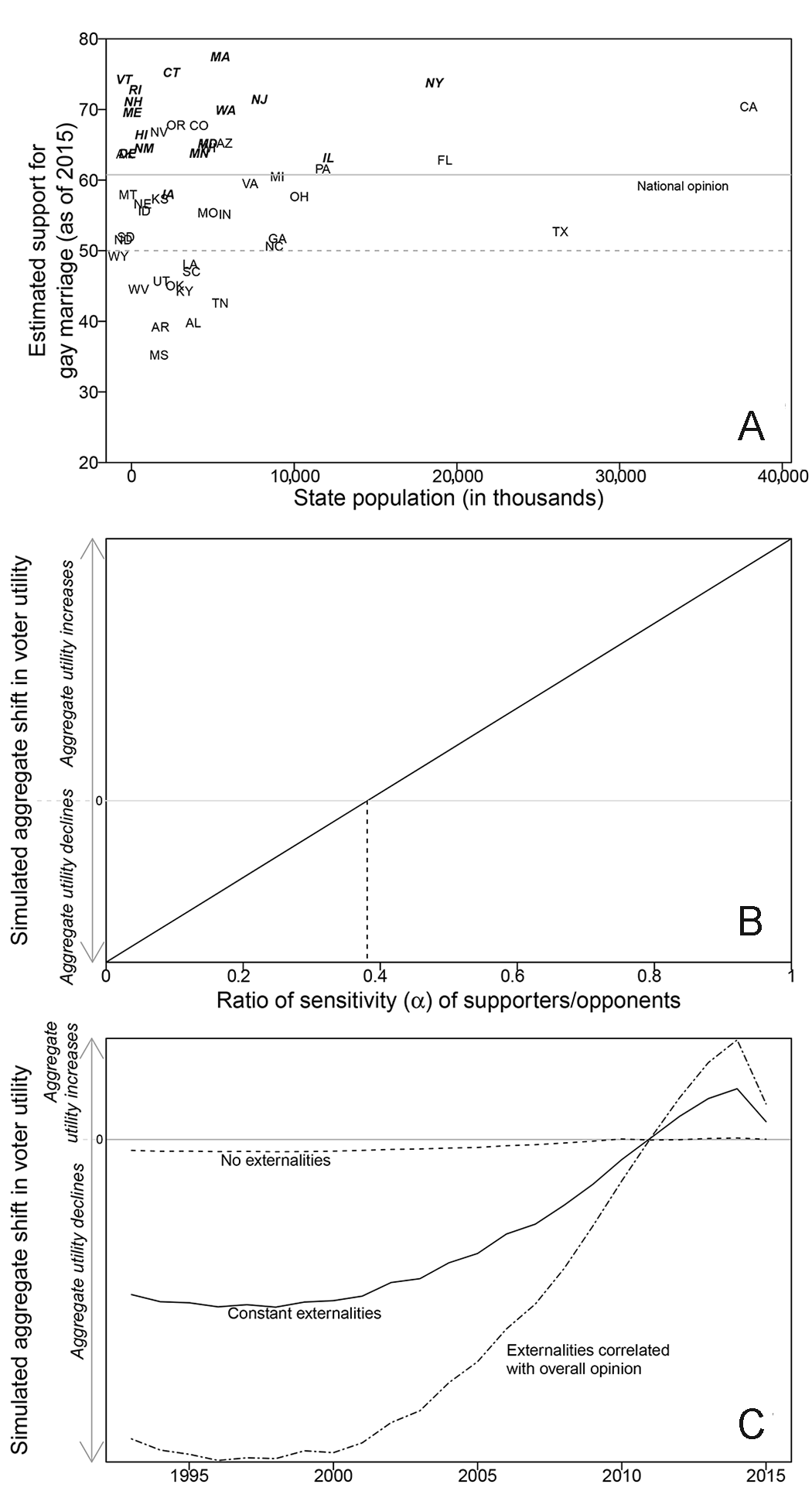
Which states, then, were “pulled in” by the federal courts? Figure 8A plots the estimated support for gay marriage in each state, as of 2015, against the size of each state (based on the 2010 census). The dashed horizontal line depicts the 50% mark, while the solid line depicts national support (62% in 2015). The states in plain text are those in which federal courts implemented gay marriage by striking down state bans, while the states in italic text already had gay marriage in place (via either legislation/referenda or state court decisions).
Role of externalities in federal courts’ implementation of gay marriage. A, Estimated support for gay marriage in each state versus the size of each state. The dashed line depicts the 50% mark, while the solid line depicts national support (62% in 2015). The states in plain text are those in which federal courts implemented gay marriage by striking down state bans, while the states in italic text are states that already had gay marriage in place (via either legislation/referenda or state court decisions). B, Simulations of the effect of voter sensitivity to out-of-state policy on overall voter welfare. C, Simulated utility over time. See text for details.
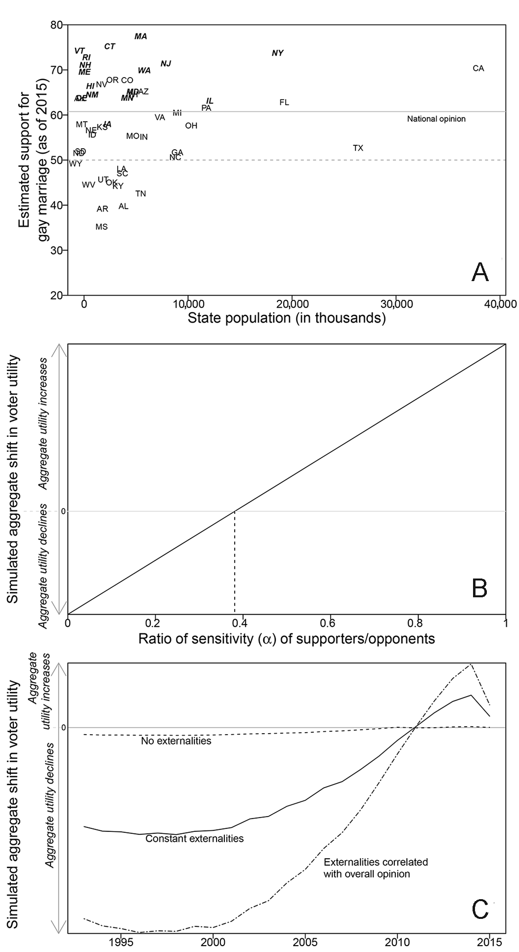
Thus, using figure 8A , we can separate the “in state” versus “out of state” effects of the introduction of federal floors. With respect to the former, as discussed earlier, the striking down of bans in states where policy lagged behind changes in public opinion (i.e., the plain-text states above the 50% line) was promajoritarian. Conversely, the implementation of gay marriage in states where opinion majorities opposed gay marriage—all of which had bans in place—was countermajoritarian. With respect to externalities, even in states where gay marriage was already in place, the introduction of federal floors induced positive externalities for supporters in these states, even though the actions of federal courts had no effect on their own state policies. Conversely, the implementation of gay marriage by federal courts created negative externalities for opponents in every state, on top of any in-state policy loss suffered where bans had been in place. Finally, while there is only a weak relationship between state size and state-level public opinion, most of the states where opinion majorities opposed same-sex marriage are below the median state in terms of population; furthermore, many of the states are in the South.
How can we weigh these positive versus negative externalities? Recall that, in the framework, α denotes the sensitivity of a voter to policy in other states. It seems unlikely that a direct measure for this quantity can be found—at least one that adequately places the sensitivity of both supporters and opponents on the same scale (as well as their joint distribution). Accordingly, I use a simulation approach to illustrate how the introduction of federal floors benefited and harmed supporters and opponents of gay marriage, and to examine the aggregate impact of these decisions.
I perform two simulation analyses. First, I create a simulated “voter-level data set,” with the number of voters in each state proportional to the actual state population (as of 2010). Then, for each “voter,” I simulate support for gay marriage, using a binomial distribution based on the estimated level of support in 2015.Footnote
18
Next, I define κ as the ratio of the sensitivity of supporters (s) of gay marriage to the sensitivity of opponents (o) (i.e.,
 ); thus, if
 , supporters and opponents weigh out-of-state policy equally.Footnote
19
For every value of κ or each voter, I then compare the “utility” before and after the introduction of a federal floor (based on eq. [5] above), taking into account the status quo in the respective states. I then calculate the overall total utility for each level of κ; I assume that if policy matches their preferences, they receive a benefit of 1 and vice versa.
The results are presented in figure 8B
. The horizontal axis depicts κ. The vertical axis depicts the simulated net utility shift from the introduction of a federal floor—similar to figure 3. The solid line indicates no net shift in utility from the introduction of the floor. Figure 8B
shows that the degree to which the introduction of the federal floor is promajoritarian is directly increasing in κ. As supporters care more about out-of-state policy than opponents, they gain more from the introduction of a federal floor than opponents lose. Due to the assumptions of the simulation, and the distribution of overall opinion in 2015, the “crossover” point at which the decision turns from counter- to promajoritarian occurs when
 .
Next, I perform a simulation analysis over time. For each year from 1993 to 2015, I again create a simulated voter-level data set, with both the proportion of voters across states and the distribution of opinion based on the actual levels in each year. Then, in every year, I calculate the overall utility shift from the introduction of a federal floor, again taking into account the status quo in each state in each year (thus, the simulations incorporate both externalities and lagging status quos). I do these calculations under three assumptions: first, voters have no cross-state externalities (
 ); second, supporters and opponents have positive but constant sensitivities (I assume
 ); third, the ratio of sensitivity for supporters versus opponents is increasing over time as a function of the distribution of national opinion in a given year.
The results are presented in Figure 8C . Each version of α shows the same substantive pattern: the introduction of a federal floor would have been countermajoritarian until a national majority favored same-sex marriage, which occurred in 2011.Footnote 20 Of greater interest, however, is that the existence of externalities has a “multiplier” effect. Under the assumption of both constant externalities and (especially) correlated externalities over time, the introduction of a federal floor early on would have been drastically more countermajoritarian compared to the assumption of no externalities, because most voters would have suffered losses from the introduction of same-sex marriage in their states as well as in all other states. Symmetrically, the introduction of a federal floor after 2011 means that many voters are doubly benefiting from the implementation of same-sex marriage both in their states and nationwide. Thus, the distribution of cross-state externalities has significant implications for how we assess the countermajoritarian nature of judicial review.
More broadly, the results in figure 8 allow us to place the implementation of gay marriage by federal courts in the larger context of federalism and the countermajoritarian difficulty. In his dissent in Obergefell, Justice Scalia argued as follows:
Until the courts put a stop to it, public debate over same-sex marriage displayed American democracy at its best. Individuals on both sides of the issue passionately, but respectfully, attempted to persuade their fellow citizens to accept their views. Americans considered the arguments and put the question to a vote. The electorates of 11 States, either directly or through their representatives, chose to expand the traditional definition of marriage. Many more decided not to. Win or lose, advocates for both sides continued pressing their cases, secure in the knowledge that an electoral loss can be negated by a later electoral win. That is exactly how our system of government is supposed to work.
It is certainly true that federal courts cut off the prospect of gay marriage being legalized at the state level with the introduction of a federal floor for the right to marry. Yet, the results above show that in many cases state opinion majorities favored legalization and benefited from federal court intervention into the policy arena. In addition, the existence of cross-state externalities, combined with the national distribution of opinion, mitigates the force of Scalia’s countermajoritarian critique.Footnote 21
V. Conclusion
In the United States, and increasingly around the world, courts have a substantial degree of political power. The federal structure of the US political system means that such power extends both horizontally and vertically. In this article, I showed that the ability of federal courts to establish constitutional floors below which states cannot set policy has real substantive bite, as it directly affects the ability of state legislatures to implement majority-preferred policies. At the same time, the existence of lagging status quos or cross-state externalities, or both, means that the introduction of federal floors can actually be welfare enhancing for voters. Thus, this article joins a burgeoning literature demonstrating how, in some (but certainly not all) circumstances, courts actually can move policy in a way that benefits opinion majorities—both within and across the states of a federation (see, e.g., Frymer Reference Frymer2003; Whittington Reference Whittington2005; Lain Reference Lain2012; Kastellec Reference Kastellec2016).
While the countermajoritarian difficulty has animated discussions of judicial review for over half a century, precise definitions of what is countermajoritarian have often been lacking, as many commentators have noted (see, e.g., Friedman Reference Friedman1993; Bassok and Dotan Reference Bassok and Dotan2013). To be sure, the framework developed here is specific, as it rests on a particular conception of what courts do and assumes a rather reduced form of utility for voters (although the framework could easily accommodate factors like the intensity of preferences and salience across issues). But the virtue of this parsimony is that it produces a clear definition of pro- versus countermajoritarianism and also provides a way to understand the nature of judicial intervention in policy development in a system of federalism and diffuse powers.
Moreover, as noted in the introduction, positive analyses of the countermajoritarian difficulty have tended to focus on the Supreme Court’s exercise of horizontal judicial review. The path to same-sex marriage illustrates the importance of considering vertical judicial review as well. First, while Congress played a role in the debate over same-sex marriage with the passage of the Defense of Marriage Act, most of the action occurred at the state level. Second, focusing solely on national opinion would mask how opposition to same-sex marriage was (by 2015) concentrated in a relatively small number of states. Viewed in this light, it is perhaps unsurprising that Obergefell generated relatively little backlash at both the state and federal levels.
Moving forward, while I mainly used the judicial federalism framework as an accounting device, the underlying architecture could be extended in a number of ways to study strategic interactions among and between judges, lawmakers, and the public, within the context of federalism. First, whereas I assumed the Supreme Court does not consider any implementation costs when establishing a federal floor, one could allow the location of the floor to be affected by the distribution of state opinion and possible noncompliance by state actors. (Such an approach, which is similar to that taken in Cameron [Reference Cameron2005], would help us understand the location of federal floors, whereas this article has focused on their effects on representation.) Second, unlike federal judges, state court judges are either elected or face reappointment, and thus their incentives to establish state constitutional floors may be directly affected by the popularity of such an implementation. Third, rather than assuming perfect compliance with federal floors, one could examine the conditions under which state lawmakers may either seek to go around them or to implement clearly unconstitutional laws that will be struck down by federal courts in an effort to “pander” to their constituents who favor such policies.
Finally, the framework could be extended to consider how litigants and activists weigh local policy gains against potential nationwide backlash. For instance, Keck (Reference Keck2009) argues that even when the early successes of the gay rights movement did provoke a negative reaction, those early victories helped engender success down the road by raising the salience of gay rights in general. Similarly, the introduction of same-sex marriage as an issue helped make civil unions an attractive “compromise” option, suggesting that activists may attempt to shift the relevant dimension over which constitutional rights are sought. Given that the emergence of new issues being debated at the state level is a pervasive feature of the US federalism system, adapting the framework along with these lines could prove fruitful for understanding the nature of policy development, and judicial reactions to that development, at the state level.
Appendix
This appendix provides information on the data and measures used in the article.
Measuring Public Opinion on Gay Marriage
To measure public opinion on gay marriage, I build on prior data and modeling by Lax and Phillips (Reference Lax and Phillips2009a, Reference Lax and Phillips2009b, Reference Lax and Phillips2012). In these papers, Lax and Phillips develop static estimates of state-level opinion of several issues related to gay rights, including same-sex marriage, using multilevel regression and poststratification (MRP)—see also Warshaw and Rodden (Reference Warshaw and Rodden2012), Bishin and Smith (Reference Bishin and Anthony Smith2013), and Lewis, Wood, and Jacobsmeier (Reference Lewis, Wood and Jacobsmeier2014). There are two stages to MRP. In the first stage, opinion is modeled as a function of demographic characteristics of respondents and geography, using random effects. In the second stage, the estimates are poststratified according to the true proportion of each “demographic-geographic” type in each state (Kastellec, Lax, and Phillips Reference Kastellec, Lax and Phillips2014).
To develop the estimates of opinion used in the article, I began with the data set of polls on gay marriage analyzed in Lax and Phillips (Reference Lax and Phillips2009b), which covered the years 1996–2008. I both backdated and updated these data in order to include every usable poll from 1993 to 2015. I did this by searching the iPoll archives (available at http://ropercenter.cornell.edu/CFIDE/cf/action/ipoll/index.cfm), using the keyword search “marr% and (gay or same-sex or homosexual).”Footnote 22 I only retained polls with questions that specifically asked about respondents views’ on same-sex marriage (and not, e.g., on whether they approved of civil unions). In addition, only polls for which individual-level data contained sufficient demographic and geographic data were retained. For each respondent, I coded race, age, gender, level of education, and state of residence. Combining the existing data with the original data left me with a “megapoll” of 69 unique polls. For computational convenience, I dropped observations with any missing data in terms of their response on the same-sex question or any of the demographic or geographic predictors used in the model detailed below; this left me with 76,064 individual responses.Footnote 23
To date, all of the MRP estimates of support for same-sex marriage (referenced above) have been static. Given the sweeping changes in public opinion on this issue in recent decades, and particularly in the period leading up to the Supreme Court’s decision in Obergefell in 2015, a dynamic approach is required. There are multiple options for accommodating changes over time in the MRP framework. One approach is that of Pacheco (Reference Pacheco2011, Reference Pacheco2014), who uses a “rolling-MRP” method to generate dynamic estimates of public opinion in several issue areas; Enns and Koch (Reference Enns and Koch2013) use a similar strategy to estimate policy mood, partisanship, and ideology at the state level over time. In this approach, separate models are estimated in either discrete or overlapping time periods (e.g., either every year or in “moving windows” of multiple years).
While useful in these applications, this approach carries limitations in other settings. First, it requires the use of polling questions that are administered at regular intervals over time; in the same-sex-marriage data I collected, there are several years with no usable polls. Second, estimating separate models over time potentially throws out useful information from the data; for instance, knowing the propensity of residents in (say) Alabama to support same-sex marriage in 1993 surely helps predict opinion in that state in 2015, even allowing for change over time.
Accordingly, I followed the general approach of Caughey and Warshaw (Reference Caughey and Warshaw2015) and Shirley and Gelman (Reference Shirley and Gelman2015) and estimated a single model that incorporates and estimates change over time. As has been well documented, national support for same-sex marriage has increased dramatically over the last 2 decades.Footnote 24 Inspection of the disaggregation measures of state opinion—that is, taking the mean level opinion for every state-year combination in the data—revealed that most states have followed a similar pattern, although the states have differed dramatically in their baseline levels of support (i.e., their “intercepts”). To account for such opinion change, I estimated a multilevel model that estimates varying intercepts for states; these intercepts are allowed to vary over time. Specifically, I included both a linear and quadratic trend in the model, which allows for the “effect” of time on opinion to vary across states.
The model also includes random effects for age, race, gender, and education; these do not vary over time. Specifically, with respect to these nonvarying random effects, I modeled response as a function of gender, one of four age groups (18–29, 30–44, 45–64, and 65+), race (white, black, and Hispanic), and one of four education groups (less than high school, high school graduate, some college, and college graduate). To provide better estimates of the state effects, I followed Lax and Phillips (Reference Lax and Phillips2009b) and include two state-level predictors. The first is the Democratic share of the two-party presidential vote, based on every presidential election between 1992 and 2012; for nonelection years, I linearly interpolated the measure based on the two closest elections (for 2013–15, I simply used the 2012 measure). The second state-level predictor is the percentage of evangelical Protestants and Mormons.Footnote 25
Formally, let i denote individual responses, and let
 denote a response in favor of support for same-sex marriage. Let n denote the number of respondents in the data. Let s, a, and e denote, respectively, indexes for states, age, and education. Let f denote the interaction of gender and race; this variable takes one of six values: female black, female white, female Hispanic, male black, male Hispanic, and male white. Next, let t denote a time trend; this variable takes the value of the year the poll was taken minus 1993 (the year of the first poll in the data set). For computational efficiency, I centered this variable by subtracting each observation from the mean in the data set and divided by 2 standard deviations, such that the average value is zero and the variable is on a similar scale to the other predictors. The square of this rescaled variable is denoted by t
2. (Rescaling also helps break the strong correlation between time and time-squared.) Denote the presidential vote share measure dem, and denote the percentage of evangelical Protestants and Mormons relig.
I estimated the following model:

The random effects are modeled as follows:
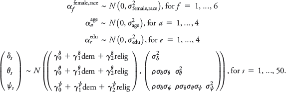
I estimated the model in a fully Bayesian manner using the program Stan, as called from R, using the rstanarm package (Gabry Reference Gabry2016; Stan Development Team 2016a, 2016b). I used weakly informative N(0,5) priors for each parameter. I ran the model on four separate chains for 500 iterations, and saved the last 250 iterations on each, to form a posterior sample size of 1,000. Standard diagnostics indicated good convergence among the four chains. For every parameter, the potential scale reduction factor was less than 1.03, and for all but seven parameters it was less than 0.01, thus indicating good mixture among the chains (Gelman and Rubin Reference Gelman and Rubin1992). The effective sample size of the parameters ranged from 227 to 1,000, the minimum was well above the recommended number (Gelman et al. Reference Gelman, Carlin, Stern, Dunson, Vehtari and Rubin2014), and for a majority of parameters the effective sample size was 1,000.Footnote 26
Poststratification
The second stage of MRP estimates requires poststratifying the results from the first-stage model, according to the true population proportion of “demographic-state” types. To do this, I used the population frequencies from the Census Public Use Microdata Area (PUMA) data for 1990 and 2000. I augmented these with data from the 2009 Census American Community Survey (the 2010 PUMA sample was never released). To estimate frequencies between these years, I used simple linear interpolation. (For years after 2009 in the opinion data, I simply used the 2009 data.) The resulting combined data set gives the estimated population frequency for every demographic-state type for every year from 1993 to 2015. (The estimates of Democratic presidential vote share and the percentage of evangelical Protestants and Mormons are then merged with these data.)
There are 4,800 combinations of demographic and state values: 50
 age
 education
 race-gender combinations. From the individual-response model, I first calculated the predicted probabilities of support for each demographic-state type, for every year. There are thus 4,800 demographic-geographic
 years (1993–2015) = 110,400 cells—which we can denote “demographic-state-year” types—in which to make a prediction. Let j denote a cell from the set of demographic-state-year types, each of which has a predicted value of supporting same-sex marriage in a given year. Denote this prediction
 , which comprises a matrix of 110,400 rows and 1,000 columns (one for each draw from the posterior distribution).
The final step is to poststratify these predictions using the estimated population frequencies from the combined census data, which we can denote Nj
. Let
 denote an estimate of support in a given state s, for each year y;
 is a matrix comprising 1,150 rows (50
 years) and 1,000 columns. Then,
 . The result is 1,000 estimates of opinion for every “state-year” combination. I used the mean estimate from the 1,000 draws to summarize the distribution of each combination.Footnote
27
The estimates of national opinion proceed comparably, except the aggregation is done at the year level:
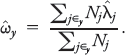
Validity Checks
As a simple validity check, it is useful to compare the MRP estimates to those produced by disaggregation—that is, simply taking the mean level of support in each state for every year. In these checks I focused solely on the point estimates of support and ignored their uncertainty.
Figure A1A depicts a scatterplot of the estimates for every state-year combination that appears in the data (i.e., combinations that are completely model-dependent are dropped). The overall correlation between the disaggregation and MRP estimates is .72 (the solid line is a 45-degree line). Of course, for many combinations with small numbers of respondents, the disaggregation estimates will suffer from large amounts of measurement error; this can clearly be seen in the cluster of points at 0 and 100. A more useful comparison is to look at state-year combinations with at least 50 respondents; most such combinations occur in the states with the largest populations, such as California, New York, and Texas. Figure A1B presents a scatterplot of the MRP and disaggregation estimates among such combinations. The correlation, at .93, is significantly stronger (and quite high in absolute terms).
As a second validity check, I followed the lead of Warshaw and Rodden (Reference Warshaw and Rodden2012, fig. 2) and conducted an external validation by comparing the MRP estimates to results from referenda on state constitutional amendments to ban gay marriage. Such referenda were held 33 times in 31 states between 1998 and 2012. Of course, those who turnout in such referenda may differ from state residents overall (i.e., those who are likely to be contacted by a national poll using a probability sample), but the results of these referenda still provide a useful benchmark for evaluating the MRP estimates.
Each plot in figure A2 evaluates the results of these referenda; the vertical axis depicts the percentage of voters who opposed a constitutional amendment to ban gay marriage in their state (i.e., 100 minus the percentage of voters who supported bans on same-sex marriage). Figure A2A plots this quantity against the disaggregation estimates of state support for gay marriage. The correlation is substantial (.72), but there are a few observations that stray significantly from the 45-degree line. Figure A2B substitutes the MRP estimates and reveals a much stronger correlation (.86); notably, the very low disaggregation estimates from smaller states (in terms of population) like Idaho and South Dakota are pooled toward the overall mean in the MRP estimates.
One potential reason for some of the discrepancies between the referenda vote and the MRP estimates is that several of the referenda also included measures to ban not just marriage but also civil unions (and, in a handful of instances, all contracts that resemble marriage-like agreements between nonmarried individuals). Such policies are more extreme than banning gay marriage, which might account for the MRP estimates for support for gay marriage being lower than opposition to a given constitutional amendment. (For example, whereas the MRP model estimates that only 31% of South Dakotans supported gay marriage in 2006, a referendum that year that proposed banning gay marriage only received 52% support; this measure, however, was of the more extreme variety.)Footnote 28 To account for this issue, figure A2C replicates A2B but only depicts the nine referenda in which same-sex marriage was the sole issue on the ballot. For such referenda, the correlation is .98, and the largest absolute difference between the vote total and the MRP estimates is 5 percentage points (the mean difference is 2.8 percentage points). Thus, in sum, the MRP estimates appear to be quite valid.
State Policy and Judicial Decisions
To measure state policy on gay marriage, I used a variety of internet and news searches to ascertain whether, when, and how each state implemented a ban on gay marriage, as well as legislation or state referenda to legalize gay marriage. Particularly helpful were the web pages put together by ProCon.org (http://gaymarriage.procon.org/view.resource.php?resourceID=004857) and the Pew Research Center (http://www.pewforum.org/2015/06/26/same-sex-marriage-state-by-state/). Klarman (Reference Klarman2012) and the references therein were also helpful.
To search for judicial decisions, I used the Westlaw key number “Marriage and Civil Unions” (92–3438). I read through the cases with this key and identified decisions that ruled on the merits of the constitutionality of a state statute. I cross-checked the resulting cases with internet and news searches; this page from FindLaw was particularly helpful: http://family.findlaw.com/marriage/developments-in-same-sex-marriage-law.html.
For decisions handed down by the courts of appeals, I identified which states in the circuit were affected by the panel’s decisions. For instance, a panel of the Fourth Circuit in 2014 struck down Virginia’s ban on gay marriage (760 F.3d 352). At that point, Maryland had legalized gay marriage via referendum in 2013. Thus, the Fourth Circuit’s decision effectively legalized gay marriage in the three other states in the circuit—West Virginia, South Carolina, and North Carolina—all of which still had bans in place as of 2014.
With respect to the US Supreme Court’s decision in Obergefell, many lower court decisions that had ruled state bans unconstitutional were stayed pending action by the Supreme Court. Thus, the Court in Obergefell technically struck down bans in these states, such as Arkansas. However, for the purposes of the empirics, I counted the original decision (be it state or district) striking down a ban as the implementing court in the respective state, since if the Supreme Court had decided not to weigh in on gay marriage (as it did for many months), those lower court decisions would have stood. Thus, Obergefell effectively reversed policy in the following seven states: Georgia, Kentucky, Louisiana, Michigan, Ohio, North Dakota, and Tennessee.
MRP estimates of support for same-sex marriage. A, Correlation of the MRP and disaggregation estimates for every state-year-policy combination that appears in the data. B, Correlation only among state-year-policy combinations with at least 50 respondents.
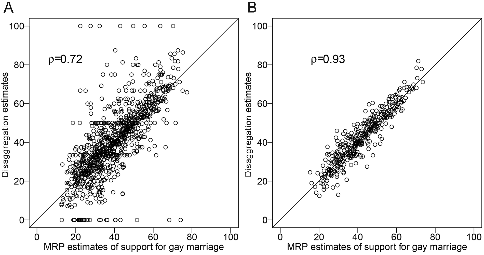
Validation of MRP estimates of support for same-sex marriage against referenda results. A, Disaggregated measures of support for gay marriage. B, MRP estimates. C, MRP estimates, looking only at referenda in which same-sex marriage was the sole issue on the ballot.