Introduction
Nanoscale heat transfer is becoming an increasingly important topic for a number of industries. From miniaturization of electronics which is reaching the nanoscale,[Reference Cahill, Braun, Chen, Clarke, Fan, Goodson, Keblinski, King, Mahan, Majumdar, Maris, Phillpot, Pop and Shi1] to the development of heat-assisted magnetic recording,[Reference Kryder, Gage, McDaniel, Challener, Rottmayer, Ganping, Yiao-Tee and Erden2] to tailoring materials and devices for thermal energy harvesting,[Reference Snyder and Toberer3] the need to reliably measure heat conduction at the nanoscale is a critical component which is currently lacking.[Reference Abad, Borca-Tasciuc and Martin-Gonzalez4,Reference Juszczyk, Kazmierczak-Balata, Firek and Bodzenta5] Scanning thermal microscopy (SThM) boasts ultra-high lateral resolution (on the order of tens of nanometers or less),[Reference Cahill, Braun, Chen, Clarke, Fan, Goodson, Keblinski, King, Mahan, Majumdar, Maris, Phillpot, Pop and Shi1] but has generally been regarded as useful for qualitative investigations only; use as a quantitative measurement tool has been met with apprehension. This may largely be attributed to a lack of consistent, reliable methods for probe-to-sample heat transfer calibration. Recent studies have demonstrated that not all calibrations yield accurate results.[Reference Wilson6–Reference Wilson, Munoz Rojo, Abad, Perez, Maiz, Schomacker, Martin-Gonzalez, Borca-Tasciuc and Borca-Tasciuc8] Therefore, in this paper, three methods for probe calibration which appear in the literature are compared: the implicit method, the step method, and the intersection method (each is described in section “State of the art calibration strategies”). Bulk reference samples with well-established thermal conductivity values are used to calibrate the probe via all three methods. With probe calibration obtained by each of these methods, the validity of each is explored by measuring the thermal conductivity of a series of film-on-substrate samples which had been previously characterized by time-domain thermoreflectance (TDTR).[Reference DeCoster, Meyer, Piercy, Gaskins, Donovan, Giri, Strnad, Potrepka, Wilson, Losego and Hopkins9] In that study, thermal conductivity of atomic-layer-deposited amorphous Al2O3 thin films on silicon (with film thickness, t f, of 2.9–202.3 nm) was determined by either treating the film as a separate layer in the heat transfer model (for t f >20 nm) or by treating the film as an extra thermal resistance at the transducer–substrate interface (for t f <20 nm). These fitting conditions were chosen as a result of sensitivity analysis on these samples. The trend in thermal conductivity versus t f was projected against expected behavior arising due to size effects on observed thermal conductivity values, and was very consistent with the modeled predictions (see Ref. [Reference DeCoster, Meyer, Piercy, Gaskins, Donovan, Giri, Strnad, Potrepka, Wilson, Losego and Hopkins9] for more details).
While TDTR is capable of resolving thermal conductivity of ultrathin films, SThM is incredibly valuable as a nanoscale thermal metrology technique given its lateral resolution, which is not limited by the laws of diffraction the way laser-based techniques and techniques that rely on photolithography are. SThM is very surface-sensitive, with the extent of the thermal penetration depth on the order of 50–100 nm for nanopatterned tips, such as those used in this work.[Reference Juszczyk, Kazmierczak-Balata, Firek and Bodzenta5] Also, SThM is non-destructive, requiring no permanent alteration of the sample. It would be incredibly valuable to establish a standard for probe calibration leading to accurate, non-destructive, sub-diffraction-resolution thermal property measurement for both bulk and thin films via SThM. The goal of this work is to establish such a standard.
State-of-the-art calibration strategies
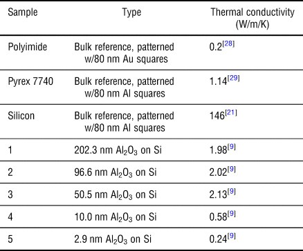
SThM may be broadly defined as a temperature measurement tool, which may be operated in active mode (A-SThM, where a self-heated probe acts as both a heater and thermometer, used for thermal conductivity mapping) or passive mode (P-SThM, where the probe is not self-heated, but is used for temperature mapping of an externally heated device or sample). A-SThM has been leveraged to measure thermal conductivity in several studies over the past two decades.[Reference Juszczyk, Kazmierczak-Balata, Firek and Bodzenta5–Reference Wilson, Munoz Rojo, Abad, Perez, Maiz, Schomacker, Martin-Gonzalez, Borca-Tasciuc and Borca-Tasciuc8,Reference Gorbunov, Fuchigami, Hazel and Tsukruk10–Reference Massoud, Bluet, Lacatena, Haras, Robillard and Chapuis16] In order to perform a quantitative measurement, the hot probe-to-sample and hot probe-to-ambient thermal exchange must be calibrated. For quantitative temperature measurement, the probe may be calibrated in P-SThM, but this paper emphasizes A-SThM calibrations for thermal conductivity measurement. The same principles for each probe calibration strategy may be applied with minor adjustments (namely, assuming no appreciable joule heating, and entering a known sample temperature which is larger than that of the probe, accounting for the difference in direction of heat flow) to achieve calibration for P-SThM temperature measurement.[Reference Chung, Kim, Hwang, Kwon, Jung, Lee, Lee and Kim17–Reference Kim, Chung, Won, Kwon, Lee, Park and Choi19] A brief summary of the calibration techniques used in A-SThM is presented in the next sections. In this paper, each of the proposed methods is vetted by measurements on three reference samples, and their ability to accurately measure the thermal conductivity of thin films is explored using a set of ultrathin film samples (3–202 nm of atomic layer deposited Al2O3 on silicon) previously measured by TDTR.[Reference DeCoster, Meyer, Piercy, Gaskins, Donovan, Giri, Strnad, Potrepka, Wilson, Losego and Hopkins9] The properties of the bulk and thin-film samples are reported in Table I.
Reference samples, surface pattern, and thermal conductivity values.

Implicit calibration
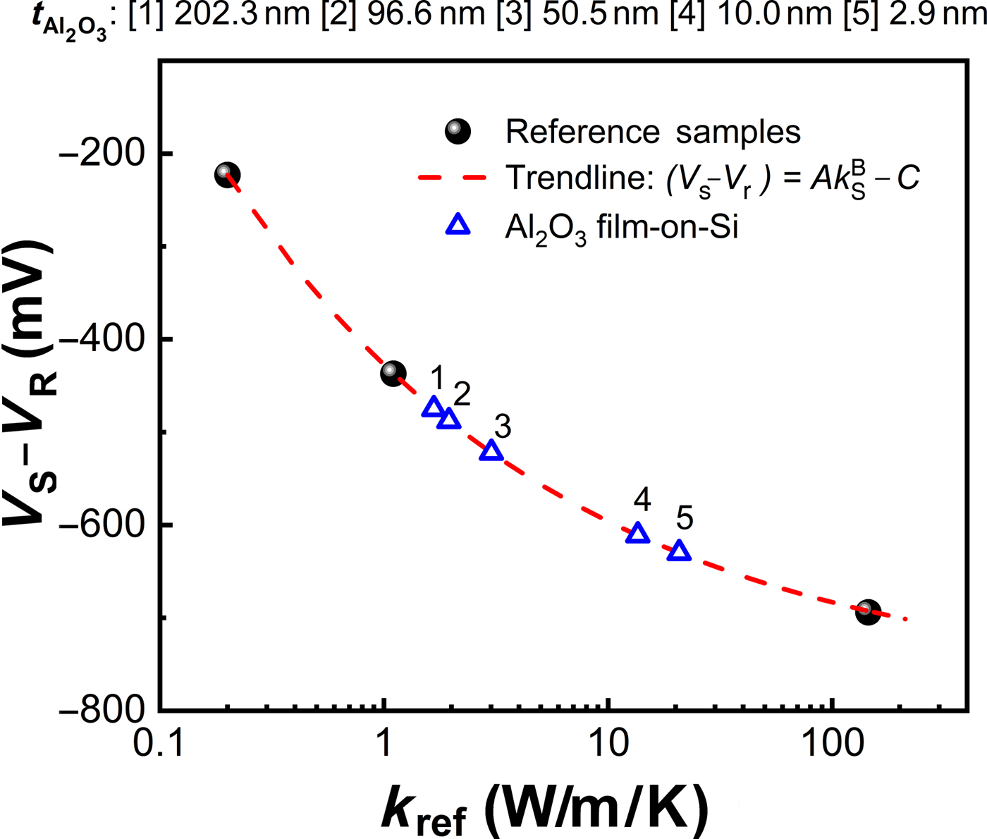
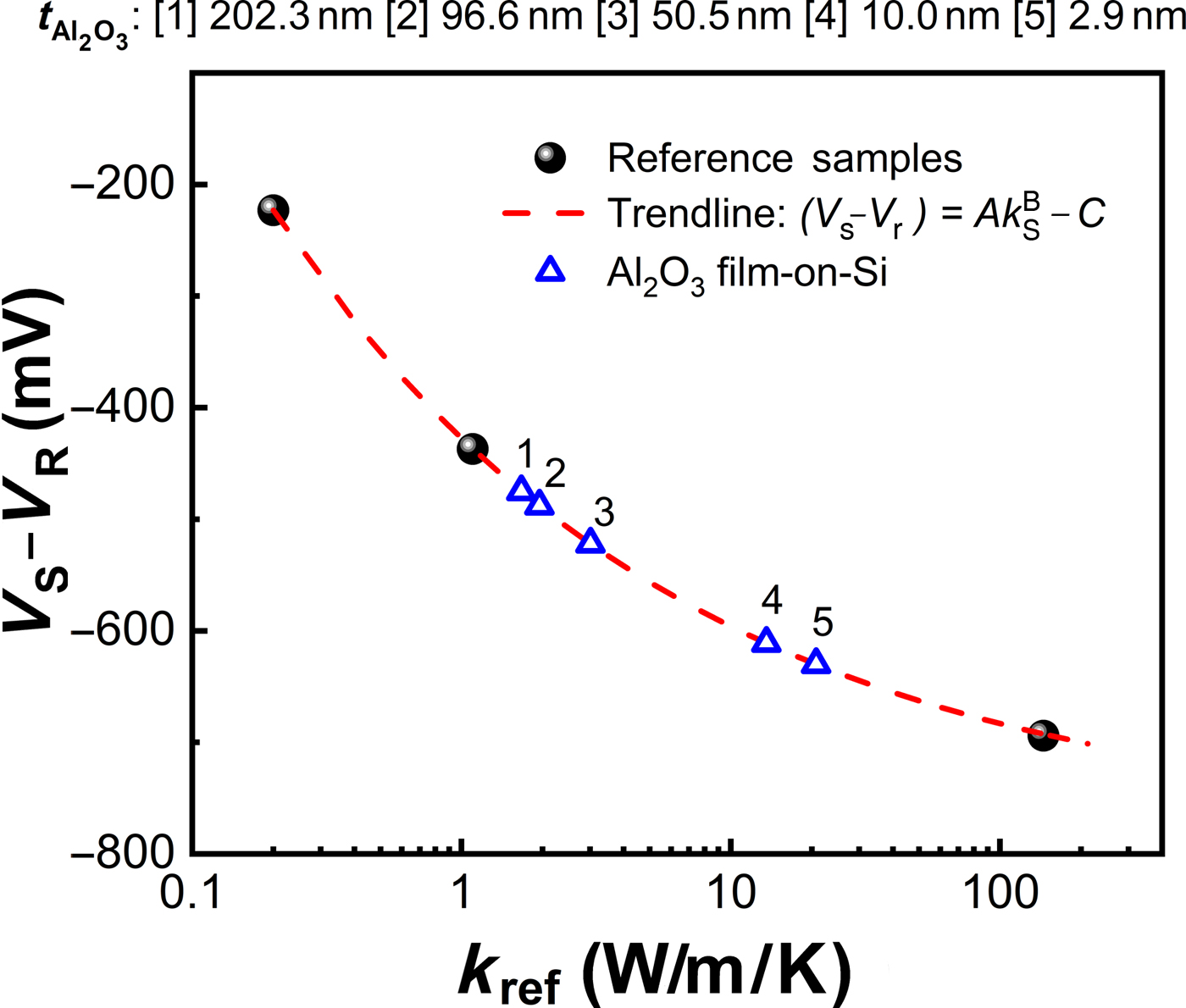
Calibrating by the implicit method, the trend in measured probe voltage signal at a given joule heating value is determined by measuring several samples with well-characterized values of thermal conductivity, then curve fitting to find the form of the equation that describes the trend.[Reference Lefèvre, Volz, Saulnier, Fuentes and Trannoy11,Reference Lefèvre, Saulnier, Fuentes and Volz20] Here, a Wheatstone bridge configuration is used. With a known value of electrical resistance in the bridge cable (R ref), the current across the probe (I P) may be readily calculated, thus probe resistance (R P) and Joule heating power  $(P_{\rm P} = I_{\rm P}^{\rm 2} R_{\rm P})$ at a given output voltage (V out) are obtained. The bridge was balanced such that the voltage across the reference side of the bridge, V r was equal in magnitude to the voltage across the measurement side of the bridge, V S. The measured signal is (V S − V r), so this corresponds to the case where (V S − V r) = 0. Then the probe was brought near to contact (roughly 1 mm above the surface, where the tip reflection comes into focus). After finding a location on the surface which was free from observable debris and topographical artifacts, the probe was brought into contact. The change in probe voltage (and electrical resistance) was observed, then the probe was removed from the sample and brought back to >25 mm above the surface. This was repeated for a range of V out, from 0.5 to 3.5 V so that the trends in resistance with Joule heating power may be obtained (discussed in section “Explicit thermal exchange calibration”). This output voltage range corresponded to 0.5–25 mA current across the probe leg of the Wheatstone bridge circuit. This was done for three reference samples with known values of thermal conductivity. The resulting graph (taken at V out = 1.5 V) is shown in Fig. 1. The curve fits the following three-parameter trend line:
 $\lpar {V_{\rm s}-V_{\rm r}} \rpar = Ak_{\rm S}^B -C$, where (V s − V r) is the measured probe voltage signal, and A, B, and C are the parameters to be fit. In this instance, A = 0.3489 ± 0.004, B = −0.2865 ± 0.004, and C = −0.7763 ± 0.003, with units such that the input units of W/m/K get converted to V. Note that confidence when employing empirical curve fitting tends to improve if we include more data points, as described in separate works,[Reference Juszczyk, Kazmierczak-Balata, Firek and Bodzenta5,Reference Lefèvre, Saulnier, Fuentes and Volz20] but three data points (owing to three unknowns in the fit) are the minimum number required to calibrate this way. Effective thermal conductivity (k eff) determination of unknown samples is demonstrated by finding thermal conductivity that gives the probe voltage values measured on the thin-film Al2O3-on-silicon samples (with V out = 1.5 V). Clearly, thicker Al2O3 leads to lower k eff (because the intrinsic thermal conductivity of Al2O3[Reference DeCoster, Meyer, Piercy, Gaskins, Donovan, Giri, Strnad, Potrepka, Wilson, Losego and Hopkins9] is much lower than silicon,[Reference Glassbrenner and Slack21] and with thicker Al2O3, less of the thermal interaction volume encompasses the substrate). Note that this strategy yields an effective (bulk-like) thermal conductivity, and to decouple the film from the substrate, the area of thermal exchange must be determined. In this work, we describe the area of thermal exchange as a circular isothermal disc, so the parameter to calibrate is the radius of that disc, b.
Implicit method for determining measured probe signal versus thermal conductivity. Curve fits take the following form:  $\lpar {V_{\rm s}-V_{\rm r}} \rpar = Ak_{\rm S}^B -C$.
Explicit thermal exchange calibration
In SThM in DC mode, R P directly correlates to the change in temperature ΔT P, as expressed by:
 $${\rm \Delta} T_{\rm P} = \displaystyle{{R_{\rm P}-R_0} \over {{\rm TCR} \times R_0}}$$
where TCR is the temperature coefficient of resistance, and R 0 is the nominal electrical resistance across the probe at room temperature. In this case, the temperature coefficient of resistance was calibrated to be 0.003/K, consistent with other studies using the same type of probe.[Reference Kaźmierczak-Bałata, Bodzenta, Krzywiecki, Juszczyk, Szmidt and Firek22] The average probe thermal resistance is determined by taking the slope of ΔT P with P P:
 $$R_{{\rm P,meas}}^{{\rm th}} = \displaystyle{{d\lpar {{\rm \Delta} T_{\rm P}} \rpar } \over {dP_{\rm P}}}$$
with calculated  $R_{\rm P}^{{\rm th}} $ from measured probe resistance, the probe-to-sample thermal exchange parameters may be explicitly calibrated by matching
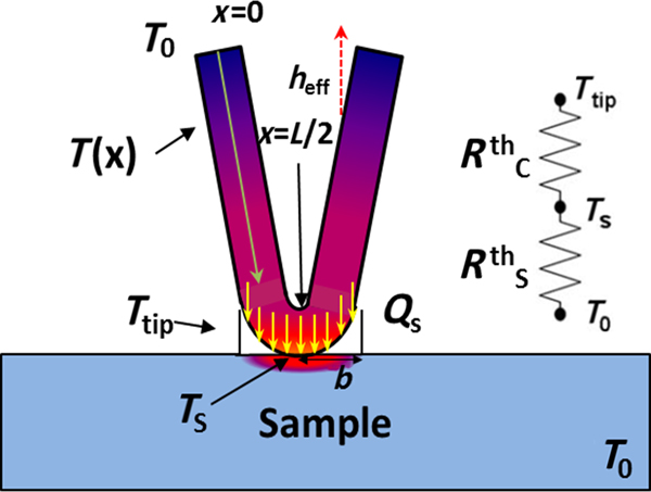
 $R_{{\rm P,meas}}^{{\rm th}} $ to that project by an analytical probe–sample heat transfer model (PSHTM). A brief summary of PSHTM is described in the next section, and is depicted schematically in Fig. 2.
Analytical model probe–sample heat transfer schematic. Reprinted from Ref. [Reference Wilson, Munoz Rojo, Abad, Perez, Maiz, Schomacker, Martin-Gonzalez, Borca-Tasciuc and Borca-Tasciuc8] with permission from the Royal Society of Chemistry, © 2015.

Analytical model derivation: salient points
The PSHTM described here has been solved several times in previous works.[Reference Puyoo, Grauby, Rampnoux, Rouviere and Dilhaire23,Reference Zhang, Hapenciuc, Castillo, Borca-Tasciuc, Mehta, Karthik and Ramanath24] Thus, the most important points are highlighted here, foregoing the full derivation. For a probe with perimeter, p, and cross-sectional area, A C, being Joule-heated by DC power, or by AC power at frequencies significantly above the probe's cut-off frequency, the probe's temperature distribution may be described by:
 $$T^{^\ast}\lpar x \rpar = C_1e^{\lambda x}-C_2e^{-\lambda x} + \displaystyle{{\rm \Gamma} \over {\lambda ^2}}$$
where  ${\rm \Gamma} = ((I_{\rm P}^2 \rho _0)/(k_{\rm p}A_{\rm C}^2 ))$,
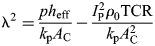 ${\rm \lambda} ^2 = \displaystyle{{ph_{{\rm eff}}} \over {k_{\rm p}A_{\rm C}}}-\displaystyle{{I_{\rm P}^2 \rho _0{\rm TCR}} \over {k_{\rm p}A_{\rm C}^2}} $, and ρ 0, k p, and TCR are, respectively, the probe's electrical resistivity, thermal conductivity, and temperature coefficient of resistance, and h eff is the effective heat transfer coefficient from the probe to the surroundings, including convective and radiative effects, and C 1 and C 2 are the constants arising from integration. Note that Eq. (3) is the temperature rise above ambient, i.e., T* = T P − T 0 where T P is the probe absolute temperature and T 0 is the temperature of the surroundings. The constants C 1 and C 2 are easily obtained by applying the two boundary conditions, defined as follows. The first assumes that where the probe meets the cantilever base, the probe is anchored to room temperature [i.e., T(0) = T 0]. The second assumes that all of the heat transferred to the sample is contained within a disc of radius b, of uniform temperature. Performing energy balance in the probe yields:
 $$\eqalign{&-k_{\rm p}A_{\rm C}\displaystyle{{dT^{^\ast}} \over {dx}} \vert _{x = L/2-b} + I_{\rm P}^2 \rho _0\lpar {1 + {\rm TCR} \times T^{^\ast} \vert_{x = L/2-b}} \rpar \displaystyle{b \over {A_{\rm C}}} \cr & \quad = \displaystyle{{Q_{\rm s}} \over 2}}$$
where b is the thermal exchange radius (i.e., the radius of the isothermal disc) and Q S is the heat transfer rate to the sample. It is convenient to define the tip thermal resistance  $(R_{{\rm Tip}}^{{\rm th}} )$, which is the intrinsic thermal resistance of the sample
 $(R_{\rm S}^{{\rm th}} )$ plus the contact thermal resistance
 $(R_{\rm C}^{{\rm th}})$ as the temperature rise in the tip region (i.e., L/2−b < x < L/2) divided by the heat transfer rate to the sample [i.e.,
 $R_{{\rm Tip}}^{{\rm th}} = \displaystyle{{T^*\vert _{x = (L/2)-b}} \over {Q_{\rm S}}} = R_{\rm C}^{{\rm th}} + R_{\rm S}^{{\rm th}} $]. Note that since the solution is for one probe leg, assuming symmetry, the temperature profile solution may be projected to both sides of the probe. Taking the integral average of the temperature profile solution,
 $$\bar{T}^{^\ast} = \displaystyle{2 \over L}\mathop \int \limits_0^{L/2} T^{^\ast}\lpar x \rpar dx$$
and rewriting as,
 $$R_{{\rm P,model}}^{{\rm th}} = \displaystyle{{{\bar{T}}^{^\ast}A_{\rm C}} \over {I^2\rho _0\lpar {1 + {\rm TCR} \times {\bar{T}}^{^\ast}} \rpar L}}$$
the model may be more readily compared with experimentally obtained values. This is a general equation for self-heated probes which develop a temperature gradient along the length of the active region, and has been applied to both nanopatterned probes with an active palladium element,[Reference Puyoo, Grauby, Rampnoux, Rouvière and Dilhaire25] as well as to Wollaston wire probes.[Reference Zhang, Hapenciuc, Castillo, Borca-Tasciuc, Mehta, Karthik and Ramanath24]
Parameters to calibrate: h eff, b, and  $\curr R_{\rm \curr C}^{{\rm\curr th}} $

The parameters in PSHTM which must be calibrated are h eff, b,  $R_{\rm C}^{{\rm th}} $, and probe geometry (p and A C). To calibrate for h eff, the probe temperature versus Joule heating power is measured in the air when the probe is far from the sample, or no sample is present. The value of h eff is then adjusted in Eqs. (3)–(6) until
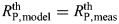 $R_{{\rm P,model}}^{{\rm th}} = R_{{\rm P,meas}}^{{\rm th}} $. Then, with a calibrated value of h eff, when inputting
 $R_{{\rm P,meas}}^{{\rm th}} $ for a sample with known thermal conductivity, the only unknowns in Eqs. (3)–(6) are b and
 $R_{\rm C}^{{\rm th}} $. The following discussions are centered on how to determine these parameters.
Step method
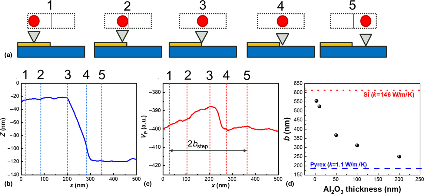
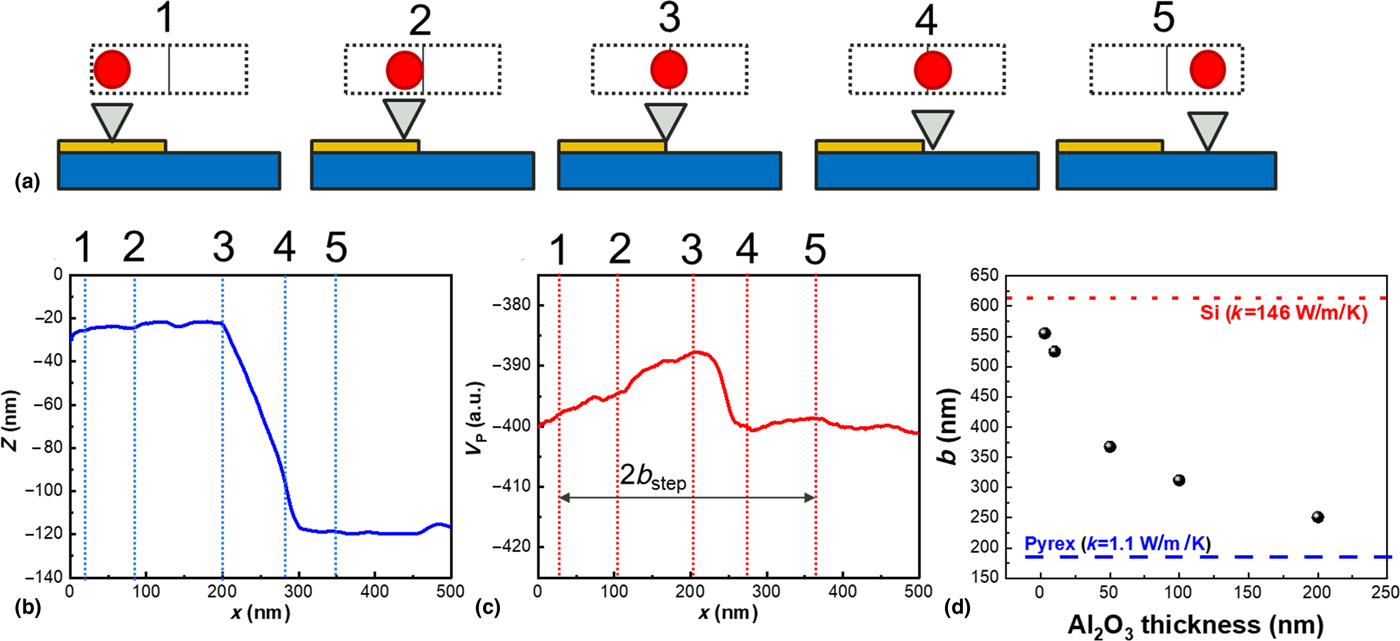
A simple solution to this problem can be obtained by measuring the thermal response of the probe as it goes over a patterned edge feature, as proposed initially by Puyoo et al.[Reference Puyoo, Grauby, Rampnoux, Rouviere and Dilhaire23] This is a strategy depicted in Figs. 3(a)–3(c). The spatial extent over which the thermal signal deviates from its behavior far from the edge is taken to be the diameter of the isothermal disc discussed in the previous section (i.e., it has the dimension 2b). This method has been used in several recent studies, both for A-SThM, as well as P-SThM.[Reference Juszczyk, Kazmierczak-Balata, Firek and Bodzenta5,Reference Kim, Chung, Hwang, Kwon and Lee18,Reference Puyoo, Grauby, Rampnoux, Rouviere and Dilhaire23] With a calibrated value of b, a reference sample with a known thermal conductivity may be measured to determine  $R_{\rm C}^{{\rm th}} $. This assumes that both b and
 $R_{\rm C}^{{\rm th}} $ are independent of the sample being measured. Recent studies have suggested that the thermal exchange radius may change as a function of thermal conductivity,[Reference Wilson6–Reference Wilson, Munoz Rojo, Abad, Perez, Maiz, Schomacker, Martin-Gonzalez, Borca-Tasciuc and Borca-Tasciuc8] so in this study, b is determined this way for all of the samples found in Table I, covering a wide range of thermal conductivity (0.2–146 W/m/K). Each of these samples had 1 mm × 1 mm patterned metal squares of ~80 nm thickness, which were used to calibrate the probe via the step method. The step calibration was performed at several values of V out, but there was no discernable difference in b with Joule heating power on any sample. However, the samples with lower thermal conductivity values demonstrated a noticeably smaller value of b compared with the higher thermal conductivity reference samples. This is depicted in Fig. 3(d). The effect of b increasing with thermal conductivity was explored in previous works by the authors,[Reference Wilson6,Reference Wilson and Borca-Tasciuc7] and was observed (without additional comment) by Kim et al.[Reference Kim, Chung, Hwang, Kwon and Lee18] However, the opposite trend (decreasing b with increasing k ref) has also been observed.[Reference Wilson, Munoz Rojo, Abad, Perez, Maiz, Schomacker, Martin-Gonzalez, Borca-Tasciuc and Borca-Tasciuc8] The apparent discrepancy may be explained by the relative contributions of the probe-to-sample heat transfer: it has been demonstrated that the nanopatterned probes transfer heat to the sample primarily across the air gap, and that high thermal conductivity samples facilitate more heat spreading across the air gap, leading to a larger thermal exchange area.[Reference Wilson6] On the other hand, the larger Wollaston probes (with which the opposite trend was observed[Reference Wilson, Munoz Rojo, Abad, Perez, Maiz, Schomacker, Martin-Gonzalez, Borca-Tasciuc and Borca-Tasciuc8]) have a larger solid contact area, which, for high thermal conductivity samples may lead to a much larger relative contribution from solid–solid conduction, which occurs only across the point of physical contact, much smaller than the area across which the heat is transferred to the sample across the air gap.[Reference Wilson6]
Calibration of thermal exchange radius, b, by the step method. (a) Schematic depicting SThM tip as it approaches and moves over the edge of the patterned feature; (b) measured z-position and (c) measured SThM probe voltage as tip moves across the edge of the patterned feature; (d) determined value of b versus Al2O3 thickness, t f, demonstrating that higher effective thermal conductivity samples show demonstrably larger thermal exchange radius by this method.
Intersection method
A calibration method that validates the probe for quantitative usage over a range of thermal conductivity values is the intersection method.[Reference Zhang, Hapenciuc, Castillo, Borca-Tasciuc, Mehta, Karthik and Ramanath24,Reference Zhang, Castillo, Mehta, Ramanath and Borca-Tasciuc26] In this method, with  $R_{{\rm P,meas}}^{{\rm th}} $ for a sample with known thermal conductivity, a value of b is assumed and plugged into Eqs. (3)–(6), and Q S is adjusted until
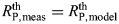 $R_{{\rm P,meas}}^{{\rm th}} = R_{{\rm P,model}}^{{\rm th}} $. That value of Q S has a corresponding value of
 $R_{\rm C}^{{\rm th}} $, so for every b a value of
 $R_{\rm C}^{{\rm th}} $ is found. Repeating this for a total of two or more reference samples each with a known thermal conductivity and plotting
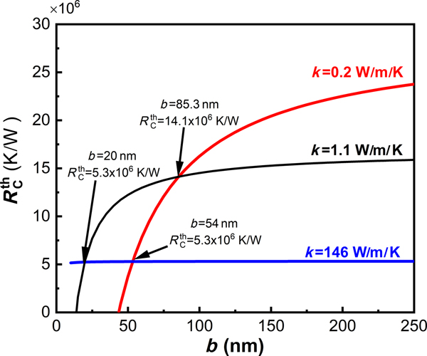
 $R_{\rm C}^{{\rm th}} $ versus b for each calibration sample, the points where the curves intersect may be found, corresponding to the calibrated pairs of (b ,
 $\; R_{\rm C}^{{\rm th}} $). This is depicted in Fig. 4. In previous studies, it was demonstrated that if thermal conductivity of the unknown sample is well outside of the range of thermal conductivity of the calibration samples, the probe calibration may no longer be valid,[Reference Wilson6,Reference Wilson, Munoz Rojo, Abad, Perez, Maiz, Schomacker, Martin-Gonzalez, Borca-Tasciuc and Borca-Tasciuc8] and a follow-on study explored the effect of sample thermal conductivity on the calibrated parameters, showing that intersections using different calibration samples do not occur in the same location, meaning that b and
 $R_{\rm C}^{{\rm th}} $ may be a function of sample thermal conductivity.[Reference Wilson and Borca-Tasciuc7]
Calibration of contact thermal resistance  ${\rm (}R_{\rm C}^{{\rm th}} {\rm )}$ versus thermal exchange radius, b. Intersections indicate a calibrated pair of
 $R_{\rm C}^{{\rm th}} $ and b.
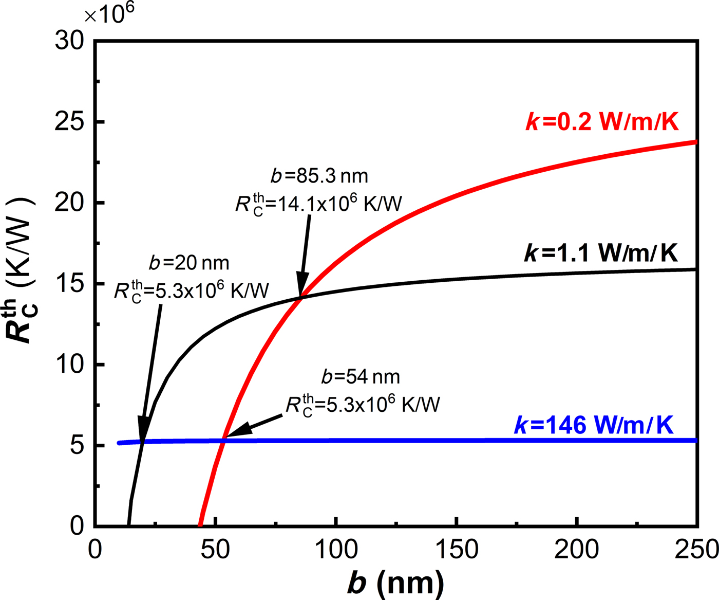
To vet the intersection method, the calibration sample set was used in contact mode. The slope of temperature with respect to Joule heating power was used as the input for the thermal resistance of the probe in each case. The resulting plot is shown in Fig. 4.
Measured thermal conductivity by probe calibration method
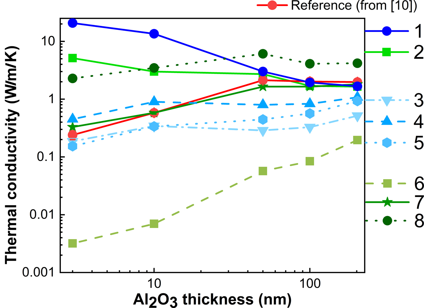
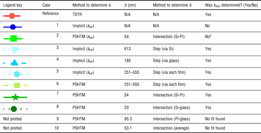
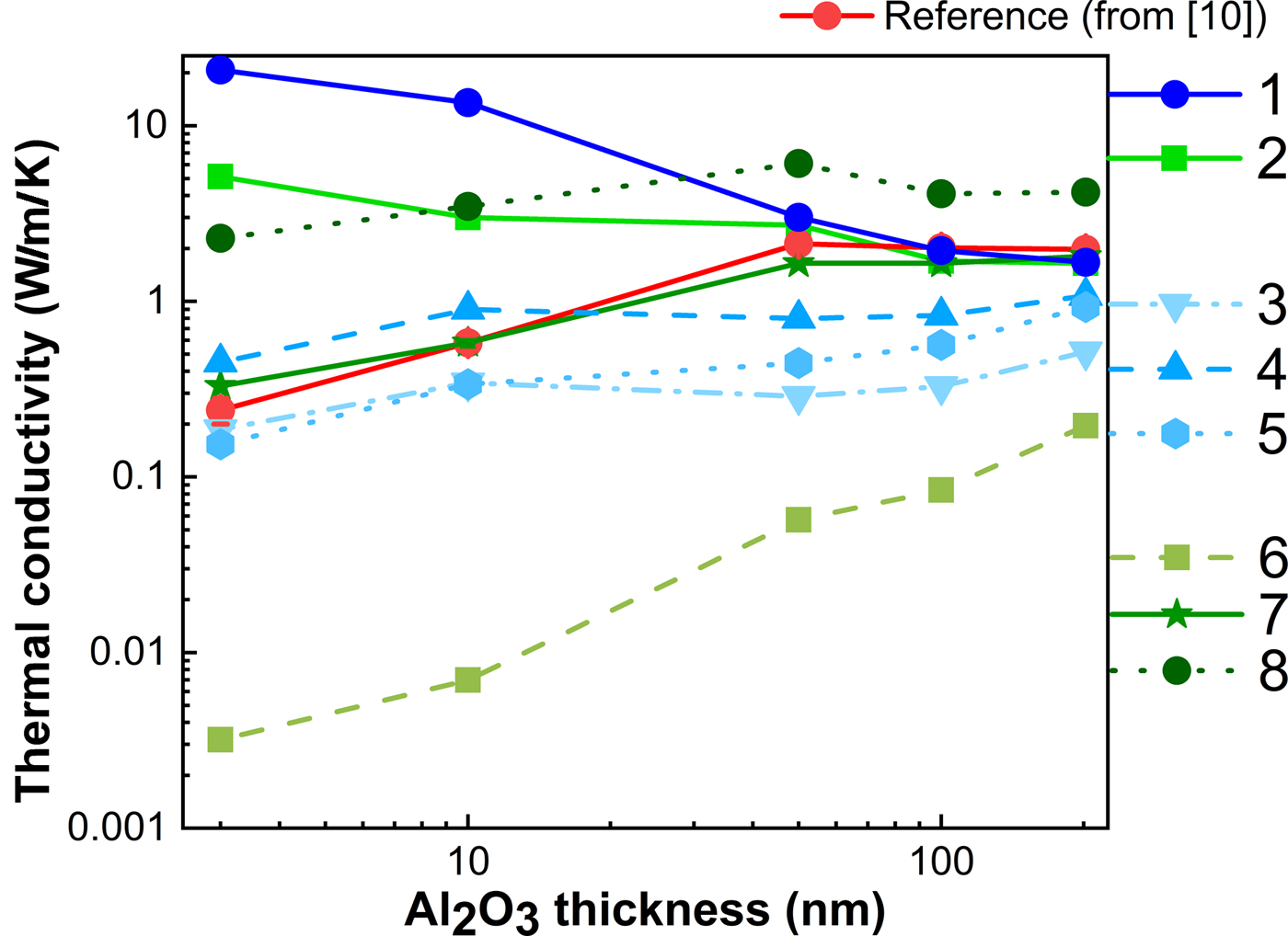
To determine the suitability of each calibration method for quantitative thermal conductivity characterization of thin-film materials, a set of samples which had been previously characterized by TDTR[Reference DeCoster, Meyer, Piercy, Gaskins, Donovan, Giri, Strnad, Potrepka, Wilson, Losego and Hopkins9] was measured by scanning the hot probe, and each of the calibration methods described in this work was used to determine the thermal conductivity of this set of samples. By default, all of these methods predict the effective (bulk) thermal conductivity, k eff [which may be correlated to the sample thermal resistance by  $R_{\rm S}^{{\rm th}} = (1/(4k_{{\rm eff}}b))$], and if t f is on the same order or less than the thermal exchange radius, the effect of the substrate must be decoupled from the film to accurately determine the film thermal conductivity. To do this, the thermal exchange radius must be explicitly determined, and a film-on-substrate model is used based on the Dryden formulation, which uses k eff, k ref, b, and t film as inputs and adjusts k film to match the total film-on-substrate thermal resistance to 1/(4k effb)[Reference Dryden27](see Supplementary Information for details on this model). The implicit method does not allow for explicit determination of b, so it must be coupled with another calibration method to determine the film thermal conductivity. On the other hand, the calibrations based on PSHTM allow for explicit determination of b by default. Using PSHTM, calibration conditions were investigated by taking b as determined by the step method, as well as by the intersection method. These results are plotted in Fig. 5, and each case tested is summarized in Table II, along with its corresponding legend key in Fig. 5.
Measured thermal conductivity by A-SThM (compared with results by TDTR) for several calibration strategies versus t f of thin-film Al2O3 on Si.
Look-up for calibration conditions and case number for film-on-substrate thermal conductivity determination.
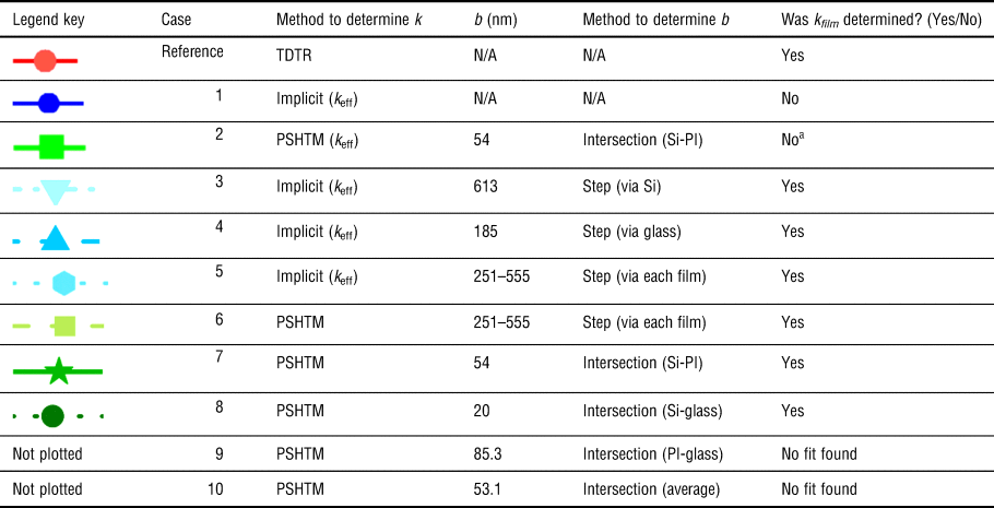
a Assuming bulk-like behavior, where 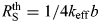 $R_{\rm S}^{{\rm th}} = 1/4k_{{\rm eff}}b$.
From the reported data, it is apparent that the effect of decoupling the film from the substrate is most pronounced for t f <50 nm, which suggests that b ≈50 nm. Cases 1 and 2 assume that the film-on substrate samples have bulk-like properties which generally match well with each other and the TDTR data for t f >50 nm, while k effincreases for t f <50 nm (while the TDTR data decrease in this range, as expected, due to size effects). This is due to the higher thermal conductivity of the Si substrate, and for thinner films, the effect of the substrate is more pronounced. Cases 3–5 combine the implicit method with b determined by the step method using different samples (as described in Table II) to decouple the film from the substrate. These data trend the same way as TDTR, but across the range, the determined value of k film is generally less than TDTR, and may deviate by more than two times. This may be due to the observed values of b being much larger than 50 nm, which would over-estimate the contribution from the substrate, causing the film to have to take a lower value to find an appropriate fit. Cases 6–8 use explicit PSHTM calibration, with 6 relying on b calibrated by the step method for each film sample, 7 taking b (and  $R_{\rm C}^{{\rm th}} $) from the intersection of Si and PI, and 8 taking b and
 $R_{\rm C}^{{\rm th}} $ from the intersection of Pyrex and Si. Each of these cases also follows a similar trend—case 6 also under-predicts k film for the same reason as cases 3–5, and case 8 over-predicts the value because in this case, b = 20 nm. The calibration using Si and PI yield, which yielded b = 54 nm, gave results that are consistent with TDTR to within 20% deviation of the previously measured values. This is consistent with the conclusions from a previous investigation which suggests that accurate results over a range of thermal conductivity (to within 20% deviation of the expected value) may be obtained by calibrating with samples having a thermal conductivity both above and below the values of interest.[Reference Wilson and Borca-Tasciuc7] Note that calibrations (cases 9 and 10 in Table II) were also obtained by the intersection method for PI and Pyrex (see Fig. 4), and the average of the three points of intersection were also taken, but due to the higher calibrated value of
 $R_{\rm C}^{{\rm th}} $ in these cases, the model yields a non-physical result, so no film thermal conductivity value was able to be determined for these cases.
Conclusions and outlook
Thermal conductivity measurements of thin films with as little as single-digit nanometer thickness by scanning the hot probe are found to be accurate when the probe calibration is performed appropriately. The intersection method using reference samples with a thermal conductivity below and above the expected k eff of the samples of interest is found to be the most accurate strategy for thin-film determination, while the step method generally follows the appropriate trends, but with values differing from the expected values by greater than a factor of two. The subjective nature of determining b by the step method makes it difficult to reply upon as a selective calibration technique, and by selection mechanism used here, the value was significantly larger than that determined by the intersection method. This work represents the first direct comparison of several widely-used strategies for probe-to-sample thermal exchange calibration, revealing that if the apparent value of thermal conductivity is taken as the correct value, this can be misleading for thin-film samples with a thickness less than the value of b. With a strategy that is self-consistent, predictive, and capable of accurately resolving thin-film thermal conductivity, quantitative usage of SThM is primed to contribute strongly to nanoscale thermal characterization efforts, which are much needed in many fields of research.
Supplementary material
The supplementary material for this article can be found at https://doi.org/10.1557/mrc.2019.37
Acknowledgments
This work was performed while the author held an NRC Research Associateship award at the US Army Research Laboratory.