2. Set-up

We study the 2-D Navier–Stokes equation governing the evolution of an incompressible velocity field $\boldsymbol {u}=(u,v)$ on the flat torus $[0,2{\rm \pi} ]^2$ with nonlinear damping, hyperviscosity and a hybrid forcing function $\boldsymbol {f}_{\!\gamma}$, namely

(2.1)\begin{gather} \partial_t \boldsymbol{u} + \boldsymbol{u} \boldsymbol{\cdot}\boldsymbol{\nabla} \boldsymbol{u} ={-} \boldsymbol{\nabla} p - \nu_n (-\nabla^2)^n\boldsymbol{u} - \beta |\boldsymbol{u}|^m \boldsymbol{u} + \boldsymbol {f}_{\!\gamma}, \end{gather}

(2.2)\begin{gather}\boldsymbol{\nabla}\boldsymbol{\cdot} \boldsymbol{u} = 0 , \end{gather}

where the integers $n$ and $m$ control the order of the hyperdiffusion and damping operators, respectively, with $n,m\geq 1$, and

(2.3)\begin{equation} \boldsymbol {f}_{\!\gamma}= \gamma \mathcal{L} [\boldsymbol{u}] + (1-\gamma)\boldsymbol{f}_{\!\epsilon}.\end{equation}

Here, the forcing control parameter $\gamma \in [0,1]$, and $\mathcal {L}[\boldsymbol {u}]$ is a linear operator whose Fourier transform is given by

(2.4)\begin{equation} \widehat{\mathcal{L}[\boldsymbol{u}]}(\boldsymbol{k}) = \nu_* k^2 \hat{\boldsymbol{u}}(\boldsymbol{k}),\quad \nu_*>0, \end{equation}

for wavenumbers $\boldsymbol {k}$ in the annulus $k=|\boldsymbol {k}| \in [k_1,k_2]$, and $\widehat {\mathcal {L}[\boldsymbol {u}] }(\boldsymbol {k})=0$ otherwise. We denote the largest length scale in the forcing range by $\ell _1\equiv 2{\rm \pi} /k_1$. This linear forcing term is associated with a maximum growth rate $\sigma \equiv \nu _* k_2^2$. An important non-dimensional number characterising this system is the ratio

(2.5)\begin{equation} r(\gamma) = \frac{\gamma\sigma}{\nu_n k_2^{2n}} \end{equation}

between the maximum instability growth rate, which occurs at the wavenumber $k=k_2$, and the rate of hyperviscous energy dissipation rate at that wavenumber. We choose $\nu _*$ such that $r(\gamma )$ varies from $r(0)=0$ to $r\gg 1$ as $\gamma$ increases from $0$ to $1$ (in all the runs described below, we take $\nu _*=0.002$, $k_2=40$, $n=4$, $\nu _4=10^{-14}$, such that $r(\gamma =1) \approx 48.8$, see table 1 for details of the parameters used). We note that the ratio $r$ has also been identified as a key control parameter in models of active turbulence (Linkmann et al. Reference Linkmann, Boffetta, Marchetti and Eckhardt2019, Reference Linkmann, Marchetti, Boffetta and Eckhardt2020), where the case $n=1$ (regular viscosity) was considered. The second term in (2.3) involves the solenoidal zero-mean white-in-time stochastic force $\boldsymbol{f}_{\!\epsilon} (\boldsymbol {x},t)$ with random phases acting within a thin shell of wavenumbers centred on the most linearly unstable wavenumber $k=k_2$, injecting kinetic energy at a rate $\epsilon$.

Table 1.

Summary of the runs performed in this study. All runs were done at a moderate resolution, $n_x=n_y=512$, to facilitate long-time integration. The parameters for the standard set-up read $\nu _* = 0.002$, $k_1=33$, $k_2=40$, $\epsilon =1$, $\beta =10^{-4}$, $n=4$, $\nu _4 = 10^{-14}$. Runs in set A are initialised from small-amplitude, random initial conditions, while runs in set B are initialised in the vortex gas state obtained in set A or vortex crystal states obtained from that by continuation in $\gamma$. In set C, the cubic damping term is replaced by a quadratic term $\beta |\boldsymbol {u}|\boldsymbol {u}$ with $\beta =0.1$, all other parameters remaining the same. In set D, the cubic damping is spectrally filtered to systematically assess its importance for the maintenance of the vortex crystal. The runs in set E are identical to runs in set A, but with the random forcing set to zero. Set F similarly repeats runs from set B with the random forcing term set to zero. Reynolds numbers given refer to the stationary state (except for set $F$) and indicate the range observed within each set.

We record the domain-averaged kinetic energy (density) $E\equiv \langle \boldsymbol {u}^2\rangle$ and the enstrophy (density) $\varOmega \equiv \langle \omega ^2 \rangle$, where $\langle {\cdot } \rangle$ denotes the domain average, as well as the vorticity $\omega \equiv \partial _x v - \partial _y u$. A further important quantity used to characterise the structure of fluid flows is the energy spectrum $E(k)$, defined by

(2.6)\begin{equation} E(k) = \sum_{\boldsymbol{q}: k-1/2\leq |\boldsymbol{q}|< k+1/2} |\hat{\boldsymbol{u}}(\boldsymbol{q})|^2, \end{equation}

which characterises the distribution of energy across scales in terms of the Fourier transform of the velocity field $\hat {\boldsymbol {u}}(\boldsymbol {q})$. The system defined above is further characterised by two dissipation-related non-dimensional parameters

(2.7a,b)\begin{equation} Re_n = U_{rms}L_I^{2n-1}/\nu_n,\quad Re_{\beta,m} = \frac{1}{\beta (U_{\mathrm{rms}})^{m-1} L_I}, \end{equation}

with the r.m.s. velocity $U_{\mathrm {rms}}=\sqrt {\langle \boldsymbol {u}^2\rangle }$ and the integral length scale $L_I$, defined spectrally as $L_I = \sum _{k} ({2{\rm \pi} }/{k}) E(k)/E$. Note that the Reynolds numbers thus defined can only be evaluated a posteriori. In addition, the problem depends on the a priori parameter $\gamma$, which controls the relative amplitude of the random and deterministic forcing terms. An alternative non-dimensional but a posteriori parameter $\varGamma$ can be defined by the ratio of the energy injection rates $\gamma \sigma U_{\mathrm {rms}}^2$ and $(1-\gamma )^{2}\epsilon$ associated with the deterministic and stochastic forces, respectively:

(2.8)\begin{equation} {\varGamma} = \frac{\gamma\sigma U_{\mathrm{rms}}^2}{(1-\gamma)^{2}\epsilon}. \end{equation}

When this parameter is large, the instability forcing provides the dominant contribution to the energy injection.

Equations (2.1)–(2.3) were solved using the MPI-parallelised, pseudospectral code GHOST (Geophysical High-Order Suite for Turbulence), cf. Mininni et al. (Reference Mininni, Rosenberg, Reddy and Pouquet2011). The 2/3 rule was used for dealiasing. We ensure that all simulations are well resolved by checking that the enstrophy dissipation rate $D_\varOmega (k) = \nu _n k^{2n+2}E(k)$ decays towards the grid scale. A total of $144$ distinct simulations were performed, requiring approximately 1 million CPU hours in total. The runs are organised in six sets as described in table 1. Cubic damping ($m=2$) is considered in all runs except those in set C, which is shown in Appendix A to yield states that are qualitatively similar to those discussed here with quadratic damping ($m=1$). All runs were done at a moderate resolution $n_x=n_y=512$ to facilitate the long-time integration required to observe the phenomena of interest here. The longest runs performed for this work (in set B) lasted approximately $40\,000$ time units measured in terms of the time scale $\sigma ^{-1}$ associated with the linear instability growth rate, corresponding to a walltime of approximately 90 days. In sets E and F, the random forcing amplitude is set to zero to isolate the impact of the random force on the observed solutions.

3. Late-time evolution near $\gamma =1$

As stated in § 1, the shielded vortex gas state described by van Kan et al. (Reference van Kan, Favier, Julien and Knobloch2022) was only followed into a dilute but transient state in which the number of vortices slowly grew owing to random vortex nucleation. In this section, we use much increased computational resources to study the long-time evolution of the system, based on runs from set A, as it converges to a statistically stationary state. Figure 1 shows snapshots of the vortex gas in the pure instability-driven case ($\gamma =1$) at different times, non-dimensionalised by the instability growth rate $\sigma$. Starting from random, small-amplitude initial conditions, a short-lived inverse cascade is followed by the emergence of shielded vortices of both parities ($\sigma t = 6.3$ in figure 1). In a stochastic competition between the two species, one is eventually eliminated leading to spontaneous symmetry breaking, as discussed by van Kan et al. (Reference van Kan, Favier, Julien and Knobloch2022). This is clearly seen at $\sigma t=378$ in figure 1. As time increases further, the number of vortices increases. The last snapshot, at $\sigma t=9312$, corresponds to the statistically stationary state. Upon inspection of figure 1, the coherent vortices are seen to be tripolar, with an elliptical core and two satellites $180^\circ$ apart. As shown by van Kan et al. (Reference van Kan, Favier, Julien and Knobloch2022), these tripolar vortices are shielded, meaning that the circulation generated by any given vortex becomes small beyond a finite radius, located close to the edge of its satellites and comparable to the largest forcing scale.

Figure 1.

Visualisation of the vorticity field at different times for $\gamma =1$, showing the evolution from small-amplitude, random initial conditions through a dilute to a dense vortex gas.

The corresponding time evolution of the enstrophy (defined in § 2) is shown in figure 2(a). This quantity is closely related to the number of vortices in this system, as shown by van Kan et al. (Reference van Kan, Favier, Julien and Knobloch2022). Four distinct phases can be identified: an initial, rapid increase of the enstrophy from small-amplitude initial conditions, associated with a short-lived inverse cascade, followed by a phase of slower, approximately linear, growth of enstrophy with time. The latter corresponds to random nucleation of new vortices in the background turbulence, depicted in figure 1. When the enstrophy reaches around $\varOmega /\sigma ^2\approx 2.5\times 10^4$ (corresponding to approximately 140 vortices in a domain of area $(2{\rm \pi} )^2$), a phase of explosive growth sets in, where the number density of vortices increases rapidly. Finally, a statistically stationary state is reached whose enstrophy is larger by a factor of approximately $2.5$ than the enstrophy threshold at which the rapid growth sets in. It should be emphasised that the observed increase in enstrophy is due to an increasing number of vortices since the core of any given vortex remains at constant vorticity due to a local balance between forcing and nonlinear damping. A similar transient evolution towards a vortex crystal in the Toner–Tu–Swift–Hohenberg model of active fluids is described by James, Bos & Wilczek (Reference James, Bos and Wilczek2018). However, in this system, the enstrophy of the final state is much smaller as a consequence of stronger nonlinear damping relative to the linear forcing strength and the time scale separation between the slow nucleation and the rapid explosive growth is therefore much less pronounced.

Figure 2.

(a) Time evolution of the enstrophy from small-amplitude random initial conditions when $\gamma =1$ (case A). (b) Colour-coded log-log plots of the energy spectrum versus wavenumber at the times indicated by dashed vertical lines in panel (a). The shaded envelopes indicate one standard deviation of the spectrum about the mean, computed over 50 snapshots. The grey shaded region indicates the forcing range.

Figure 2(b) shows a log-log plot of the energy spectrum $E(k)$ versus the wavenumber $k$ at the times highlighted in panel (a) by vertical dashed lines. The spectrum shown is averaged over 50 consecutive snapshots, with the shaded envelope indicating one standard deviation around the mean. At the earliest time illustrated, $\sigma t =378$, the energy spectrum has a local maximum at the largest scale, a remnant of the short-lived early-time inverse cascade. As time passes, the kinetic energy in the large scales continuously decreases and a sharp local maximum appears at an intermediate scale, approximately twice the forcing scale, and corresponding to the scale of the individual vortices.

Figure 3(a) shows the non-dimensional enstrophy (compensated by $\gamma$) versus the non-dimensional time $\sigma t$ for $\gamma =0.8$, 0.85, 0.9, 0.95, and 1. In addition to the run at $\gamma =1$ already shown in figure 2, we generated an ensemble of $10$ runs which differed only in the phases of their random, small-amplitude initial conditions. Similarly, at $\gamma =0.95$, we performed $10$ additional runs which also differed in the phases of their random, small-amplitude initial conditions and in the realisation of the stochastic forcing (by construction, no stochastic forcing is present at $\gamma =1$). Several things can be gleaned from figure 3(a). First, the explosive nucleation of new vortices seen in figure 2(a) is triggered when the enstrophy reaches $\varOmega \sim 0.4\varOmega _{max}$, in terms of the enstrophy $\varOmega _{max}$ attained in the stationary state, regardless of the value of $\gamma$ (horizontal dashed line in figure 3a). In fact, random vortex nucleation was observed for $\gamma \gtrsim 0.6$ (van Kan et al. Reference van Kan, Favier, Julien and Knobloch2022), but the late-time dynamics for $0.6<\gamma <0.8$ remained numerically inaccessible owing to the excessively long simulation time required to reach the final statistically stationary state at these parameter values. Second, the enstrophy in the statistically stationary state scales linearly with $\gamma$ to a good approximation between $\gamma =0.8$ and $\gamma =1$. This is consistent with a dominant balance between the instability forcing term, which is linear in the velocity, and the cubic damping term in (2.1). In contrast, the time scale $t_{exp}$ required for the system to reach the explosive phase exhibits a non-trivial, sensitive dependence on $\gamma$ whose origin remains unclear. For the parameters considered here, the threshold configuration (shown in figure 1 at $\sigma t=5980$) contains approximately $140$ vortices in a domain of area $(2{\rm \pi} )^2$, see also figure 13. We note that the mean distance $d_{NN}$ between the vortex centres of nearest neighbours (computed by finding the nearest neighbour of any given vortex, and averaging over the population and over time) close to this threshold is approximately $d_{NN}\approx 2\ell _1$, which is somewhat larger than the integral scale (defined in § 1), which is given by $L_I\approx 1.4\ell _1$ (with $\ell _1=2{\rm \pi} /k_1$).

Figure 3.

(a) Nearly self-similar evolution of the enstrophy from small-amplitude random initial conditions to the dense vortex gas. The final enstrophy value in the stationary state scales approximately linearly with $\gamma$, while the time scale depends on $\gamma$ highly nonlinearly. Low-opacity curves at $\gamma =1$ and $\gamma =0.95$ indicate an ensemble of ten runs performed at each of these values. The horizontal dashed line indicates the enstrophy threshold for the onset of the rapid growth phase. (b) Zoom on early times highlighting the stochastic nature of the evolution and the deviations between different ensemble members. (c) Non-dimensional time $\sigma t_{exp}$ at which the explosive growth phase begins versus $\gamma$. An empirical power law with an exponent between $-7$ and $-8$ is observed. Inset shows non-dimensional duration $\sigma t_{growth}$ of the explosive growth phase versus $\gamma$, where $t_{growth}$ is defined as the difference between $t_{exp}$ and the time required for the enstrophy to reach $90\,\%$ of its maximum value at a given $\gamma$. The results show a significantly weaker dependence of $t_{growth}$ on $\gamma$ compared to $t_{exp}$. (d) Near self-similarity is verified by replotting the data from panel (a) against a time rescaled by $t_{exp}$, with colours being consistent between the two panels. Since $t_{exp}$ increases with $\gamma$ significantly faster than $t_{growth}$, the rapid growth phase appears to sharpen as $\gamma$ decreases under this rescaling.

Figure 3(b) shows a zoom on the early phase of the evolution, highlighting the stochasticity of the nucleation process. Figure 3(c) shows the time $t_{exp}$ required to reach $40\,\%$ of the statistically stationary state enstrophy, where the phase of explosive growth is triggered, for all the simulations shown in panel (a), with the dashed line indicating a power-law fit giving an empirical exponent approximately equal to $-7.6$. To date, no theoretical argument for such a power-law dependence has been identified. The inset in panel (c) shows the duration $t_{growth}$ of the explosive growth phase as a function of $\gamma$ for the same runs. This time depends on $\gamma$ less strongly than $t_{exp}$, with a power-law fit with an approximate exponent of $-2.2$ although the data show a significant spread within ensembles. Figure 3(d) shows the same data as panel (a) but with time rescaled by $t_{exp}$, confirming the near self-similarity of the nucleation process. Since the duration $t_{growth}$ of the explosive growth phase is not proportional to $t_{exp}$, the collapse during the latter phase is imperfect. Moreover, the scaling of the stationary-state enstrophy with $\gamma$ is seen to be satisfied only approximately.

The increasingly slow nucleation of new shielded vortices as $\gamma$ decreases is a reflection of time scale competition. As $\gamma$ decreases, the time scale for the generation of a new vortex by the linear instability increases. The background turbulence, taking place in the interstitial space between the vortices already present, generates shear which disrupts the formation of new vortices and hence it may be expected that vortex nucleation slows down as $\gamma$ decreases. For different values of $\gamma$, we measured the average strain rate $\|\boldsymbol {D}\| \equiv \sqrt {\mathrm {tr}(\boldsymbol {D} \boldsymbol {D}^{\rm T})}$, where $\boldsymbol {D} \equiv \frac {1}{2}(\boldsymbol {\nabla } \boldsymbol {u} + (\boldsymbol {\nabla } \boldsymbol {u})^{\rm T})$ is the rate of strain tensor, and the average mean-square vorticity of the turbulence in the interstitial space of the dilute vortex gas (not shown). We found that both of these quantities are much larger than the maximum instability growth rate, indicating that nucleation of new shielded vortices from this turbulent background is indeed a rare event. In principle, one may hope to deduce the dependence of $t_{exp}$ on $\gamma$ from these considerations. However, the fact that the interstitial turbulence is no longer homogeneous owing to the embedded coherent, shielded vortices complicates the picture.

As illustrated by figure 4(a), there is a tendency for large-amplitude vorticity fluctuations to occur in the vicinity of coherent vortices. This is likely a manifestation of the coherent vortices imparting vorticity to their vicinity through filamentation or diffusion. Therefore, during the random nucleation process, as the coherent vortices increase in number, and the interstitial space is reduced, the amplitude of vorticity fluctuations in the interstices increases. This is confirmed by the time evolution of the mean-squared interstitial vorticity, shown in figure 4(b). The mean-squared vorticity in the interstices is indeed seen to increase over time during the random nucleation process. At the threshold of around two-fifths of the final enstrophy, a value that appears to be universal across $\gamma$, the interstices are sufficiently reduced in size that high-amplitude vorticity fluctuations can rapidly develop, serving as seeds for new shielded vortices, allowing rapid nucleation of the remaining three-fifths of the final number of vortices (note that only vortices of the same sign can mature in the vortex gas past the initial stage of spontaneous symmetry breaking, since vortices of the opposite sign undergo destructive interactions as discussed by van Kan et al. Reference van Kan, Favier, Julien and Knobloch2022). This type of explosive nucleation resembles behaviour observed in systems undergoing crowd synchronisation via quorum sensing when a large number of dynamical elements communicate with each other via a common information pool (Strogatz et al. Reference Strogatz, Abrams, McRobie, Eckhardt and Ott2005; Zamora-Munta et al. Reference Zamora-Munta, Masoller, Garcia-Ojalvo and Roy2010), here the interstitial vorticity. Although the initial spontaneous symmetry breaking occurs rapidly compared with the slow nucleation process in the runs discussed here, at smaller values of $\gamma$, there can be significant transients during which vortices of both signs coexist in the domain (van Kan et al. Reference van Kan, Favier, Julien and Knobloch2022). This is compatible with the findings of James et al. (Reference James, Suchla, Dunkel and Wilczek2021) in active turbulence at moderate Reynolds numbers, who report similar transients with subdomains of locally aligned vortices, whose duration grows with the size of the domain. In the present work, we focus instead on the behaviour at substantially larger Reynolds numbers in a large domain of a fixed size, leaving the domain size dependence to future work.

Figure 4.

(a) Snapshot of the vorticity field at $\gamma =1$ during the random nucleation process, highlighting the interstitial vorticity field by filtering out regions where the strain amplitude $\|\boldsymbol {D}\|$ (defined in the main text) is larger than $5\,\%$ of its maximum value (we have also tested other threshold values and found qualitatively the same results). High-amplitude vorticity fluctuations are preferentially found in the vicinity of shielded vortices. (b) Time series of the mean squared vorticity at $\gamma =1$, averaged over the interstitial space between the coherent vortices, computed from the vorticity field shown in panel (a). The mean squared interstitial vorticity increases in time in a manner reminiscent of the full enstrophy shown in figure 3, with the observed interstitial values significantly smaller than the total enstrophy that is dominated by the coherent vortices. The growth in interstitial vorticity indicates that within the shrinking gaps between the coherent vortices, vorticity fluctuations increase in strength over time.

As $\gamma$ changes, the relative importance of the two terms in the forcing function also changes. To determine which term is responsible for setting the observed increasingly long time scales of the approach to the stationary state, we compare two ensembles of runs at $\gamma =0.95$ from sets A and E defined by the presence or absence of the random forcing term (cf. § 2). The late-time evolution of enstrophy in these two ensembles is shown in figure 5. The deviation between the average $t_{exp}$ in the two ensembles is not statistically significant compared with the standard deviation. In addition to the simulations at $\gamma =0.95$, we have also performed a run without random forcing at $\gamma =0.8$ (not shown), and found that in this case, the evolution of the enstrophy with and without the stochastic forcing is also nearly identical. These findings indicate that, at least for $\gamma$ close to unity, the stochastic forcing plays only a minor role in setting the transition to the dense state. This is consistent with the observation that the ratio $\varGamma$ (defined in (2.8)) between the energy injection rate associated with the instability forcing term and the random force is much greater than one. Specifically, we find that, in the stationary state, $\varGamma (\gamma =0.8)\approx 4.4\times 10^4 \gg 1$.

Figure 5.

Time series of enstrophy from two ensembles of runs at $\gamma =0.95$. In the first ensemble, shown by the green curves, the random forcing is switched on with $\epsilon =1$ (same data as in figure 3), while in the second ensemble, shown by the brown curves, the random forcing amplitude is set to zero, $\epsilon =0$. The difference between the average of $t_{exp}$ over each of the two ensembles is not statistically significant compared with the standard deviation.

4. Crystallisation transition at small $\gamma$

The dense vortex gas states found near $\gamma = 1$, whose emergence was described in the previous section, can be continued to smaller values of $\gamma$, where the observed states become much more regular. This behaviour may appear unexpected, given that reducing $\gamma$ implies stronger stochastic forcing relative to instability forcing. However, for all the results described below, the instability forcing term remains dominant in the sense that the ratio $\varGamma$ remains large. 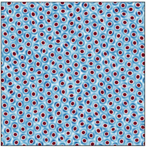The dependence of the late-time flow state on $\gamma$ is illustrated in figure 6, where snapshots of the vorticity field are shown for runs in set B at $\gamma =1$, $\gamma =0.5$ and $\gamma =0.05$. In the latter case, a spontaneously formed hexagonal vortex crystal is observed. For identical point vortices, this is the only stable vortex lattice in a periodic domain (Tkachenko Reference Tkachenko1966). In all three panels, the vortices are of one sign only, i.e. all three panels represent symmetry-broken chiral states. However, for every state shown in figure 6, there exists a corresponding state with the sign of the vorticity reversed. The vortex state shown in figure 6(a,b) at high Reynolds numbers differs substantially from the disorganised, active turbulence state described by James et al. (Reference James, Suchla, Dunkel and Wilczek2021) for moderate Reynolds numbers, since we observe only vortices of a single sign, all with a pronounced tripolar structure and therefore shielded. The vortex crystal shown in figure 6(c) bears some resemblance to the active vortex lattice of James et al. (Reference James, Suchla, Dunkel and Wilczek2021), although in the latter, vortices are not tripolar, but rather embedded in a background of uniform but opposite vorticity.

Figure 6.

Snapshots of the vorticity field in the dense, statistically stationary state at: (a) $\gamma = 1$; (b) $\gamma =0.5$ and (c) $\gamma =0.05$.

In the following, the transition from the disordered vortex gas to the crystal is analysed quantitatively using different methods from statistical physics and crystallography.

4.1. Vortex diffusion

Supplementary movies SM1, SM2, SM3 available at https://doi.org/10.1017/jfm.2024.162 show the evolution of the vorticity field over time for $\gamma =0.5,0.25$ and $0.05$. As $\gamma$ is reduced, the root-mean-square speed at which individual vortices traverse the domain decreases significantly. In particular, one observes that the individual vortices in the gas phase move chaotically across the domain but are trapped in the crystalline state. Therefore, the speed at which individual vortices propagate through the domain is a natural order parameter for quantifying the transition to the crystalline state. A particle-image-velocimetry (PIV) algorithm (Adrian & Westerweel Reference Adrian and Westerweel2011) is suitable for this purpose.

We have implemented such an algorithm in Python and applied it to the dense vortex states, taking into account the complicating feature of the periodic boundaries, which can lead to spurious doppelgängers that must be eliminated to obtain the correct trajectories. This procedure yields trajectories such as those shown in figure 7, where each colour represents the trajectory of a single vortex in the system, shifted to start at the origin and extending from $t=0$ to $\sigma t = 300$. At $\gamma =0.5$ and $\gamma =0.25$ (figure 7a,b), the vortices diffuse with a mean squared displacement that increases with $\gamma$. By contrast, at $\gamma =0.05$ (figure 7c), i.e. in the crystalline state, the vortices remain trapped close to the origin.

Figure 7.

Trajectories of all individual vortices in the system from $t=0$ to $\sigma t = 300$, shifted to start at the origin, for (a) $\gamma =0.5$; (b) $\gamma =0.25$ and (c) $\gamma =0.05$. Each colour indicates the trajectory of a particular vortex. The vortices diffuse above the melting transition ($\gamma \geq \gamma_c\approx 0.13$) at a rate that increases with $\gamma$, but are trapped at $\gamma = 0.05$ (crystalline state).

To quantify this impression, we compute the mean squared displacement, a classical measure in the study of diffusion processes, over the vortex population as a function of time. Regular diffusion, which can be microscopically realised by Brownian motion, is characterised by a linear increase of the mean squared displacement with time (Einstein Reference Einstein1905). The forced-dissipative system we are considering here is out of equilibrium, even if only weakly so, owing to the absence of an inverse energy cascade. Random motions observed in out-of-equilibrium systems are often characterised by anomalous diffusion (Metzler & Klafter Reference Metzler and Klafter2000; Sokolov & Klafter Reference Sokolov and Klafter2005), defined by a nonlinear scaling of the mean squared displacement with time.

Against this backdrop, the results shown in figure 8(a) can be considered surprising: the complex mutual advection of individual vortices leads to a mean squared displacement that increases approximately linearly with time, i.e. the vortices perform regular diffusion. The (non-dimensional) slope $D_v$ of the mean squared displacement over time is shown in panel (b) as a function of the forcing parameter $\gamma$. Below a critical threshold, $\gamma =\gamma _c\approx 0.13$, individual vortices are trapped in the vortex crystal. Above this threshold, the diffusivity increases monotonically with $\gamma$. The dashed line indicates a quadratic fit near the onset of diffusion, which is accurate from $\gamma =\gamma _c\approx 0.13$ to $\gamma \approx 0.25$. The transition is seen to be continuous (or supercritical). Figure 8(c) shows the same data as panel (b), but as a function of $\varGamma$, defined in (2.8). The crystallisation transition occurs at $\varGamma =\varGamma _c\approx 90$ with a critical exponent close to one. Similar behaviour is found in other systems exhibiting hexagonal symmetry (Ammelt, Astrov & Purwins Reference Ammelt, Astrov and Purwins1998; Bortolozzo, Clerc & Residori Reference Bortolozzo, Clerc and Residori2009; Ophaus et al. Reference Ophaus, Knobloch, Gurevich and Thiele2021) but appears unrelated to any of the classical instabilities of a hexagonal pattern such as Eckhaus, zigzag or varicose instabilities (Sushchik & Tsimring Reference Sushchik and Tsimring1994; Echebarria & Riecke Reference Echebarria and Riecke2000). In the following, we refer to the transition from trapped to diffusive vortex motion observed at $\gamma =\gamma _c$ interchangeably as a crystallisation transition or a melting transition. The observation that the melting transition discussed here is continuous is particularly interesting in view of the large literature on the search for similar continuous melting transitions in particle systems at equilibrium (Dash Reference Dash1999).

Figure 8.

(a) Mean squared displacement of vortices at different $\gamma$ versus time. The observed increase is approximately linear. (b) Blue circles represent the slope $D_v$ measured from the observed mean squared displacements versus $\gamma$. Error bars indicate uncertainty in slope estimation. A clear threshold for crystallisation can be discerned at $\gamma =\gamma _c\approx 0.13$. Black dashed line shows a quadratic fit in $\gamma -\gamma _c$ which is consistent with the data near onset. Inset shows a log-log plot of $D_v$ versus $\gamma -\gamma _c$, validating the approximate agreement between the data and the quadratic fit. (c) Same data as in panel (b), shown as a function of the ratio $\varGamma$ (defined in (2.8)) of energy injection rates due to instability and random forcing. The slope $D_v$ scales approximately linearly with $\varGamma -\varGamma _c$, where $\varGamma _c\approx 90$.

In Appendix C, the location of this transition is shown to be insensitive to the width of the wavenumber band on which the random forcing acts. It is further highlighted there that in the absence of the random forcing ($\epsilon =0$), the vortex crystal develops defects which lead to residual diffusion that makes the sharp transition of figure 8 imperfect. Thus, the role of the noise associated with the stochastic forcing term in this system is once again counterintuitive, although it is well known that in simpler situations, noise can indeed promote synchronisation, both in chaotic systems (Zhou & Kurths Reference Zhou and Kurths2002) and in systems of non-identical units including phase-coupled oscillators (Nagai & Kori Reference Nagai and Kori2010).

4.2. Radial distribution functions

Another well-established measure of structured particle systems in statistical physics is the radial distribution function, usually denoted by $g(r)$ (Chandler Reference Chandler1987). This quantity, also referred to as the pair correlation function or pair distribution function, measures the average density of particles near some location $\boldsymbol {r}$ with $|\boldsymbol {r}|=r$, given that a tagged particle is located at the origin. An equivalent definition of $g(r)$ is as the probability density of the quantity $N(r)/r$, where $N(r)$ is the number of vortices found within a radius $[r,r+dr]$ of a given vortex. The radial distribution function allows one to quantify the state of matter in particle systems and has been used to characterise active vortex crystal states (Riedel et al. Reference Riedel, Kruse and Howard2005).

Figure 9 shows the radial distribution function observed in our system in the crystalline state and above the melting transition. In panel (a), corresponding to the crystalline state at $\gamma =0.05$, there are pronounced peaks near $r\approx 2\ell _1$ (nearest neighbour distance), $r\approx 2\sqrt {3}\ell _1$ (next nearest neighbour), $r\approx 4\ell _1$ (next next nearest neighbour) and this structure continues to larger radii, modulo increasing fluctuations. Figure 9(b) shows that a liquid-like structure is observed beyond the melting transition, with a clear peak near the minimum distance between vortex centres, associated with the finite size of the vortices, and successive peaks at larger radii indicating different coordination shells (Chandler Reference Chandler1987). A zoom on the first peak highlights that it decreases in radius as $\gamma$ increases, in agreement with direct measurement of the average vorticity profile, as shown in figure 12 below. At large separations, $g(r)$ becomes constant, reflecting the random arrangement of vortices in the vortex gas, which might also be called a vortex liquid in view of this result. Indeed, it is known that a dense system of vortices can be treated as a fluid and can itself be described in terms of anomalous hydrodynamics (Wiegmann & Abanov Reference Wiegmann and Abanov2014), although these authors only consider point vortex flows and do not include the effects of shielding or of the finite size of individual vortices.

Figure 9.

Radial distribution function $g(r)$ for different values of $\gamma$ in the vortex crystal state at (a) $\gamma =0.05$ and (b) for values of $\gamma$ above the melting transition. In the crystalline state, there are pronounced peaks in $g(r)$ at nearest-neighbour, next-nearest-neighbour and next-next-nearest-neighbour distances (indicated by NN, NNN, NNNN, respectively). In panel (b), a liquid-like structure is observed beyond the melting transition. The inset shows a zoom on the first peak, which is seen to shift to smaller radii as $\gamma$ increases, reflecting shrinking vortex size.

The regularity or irregularity of dense vortex configurations in different phases can also be measured using Voronoi diagrams, as described in Appendix B. One result of this analysis is that the inter-vortex distance decreases as $\gamma$ increases. However, the Voronoi analysis is based purely on the location of vortex centres and does not include information about the vorticity structure or the vortex size. This analysis thus cannot distinguish between larger gaps between vortices and a change in the vortex size.

4.3. Lindemann ratio

Further insight into the physics of the melting transition of the vortex lattice can be gained by considering the relative displacements of vortices. This can be quantified using an established criterion in terms of the non-dimensional Lindemann ratio (Goldman et al. Reference Goldman, Shattuck, Moon, Swift and Swinney2003), given by

(4.1)\begin{equation} r_L = \frac{\langle |u_m-u_n|^2\rangle}{a^2}, \end{equation}

in terms of the lattice spacing $a$, where $u_m$ is the displacement of vortex $m$ from the perfect lattice and the average is over nearest-neighbour vortex pairs indexed by $m,n$. In simulations of 2-D crystalline atomic lattices at thermal equilibrium, melting has been found to occur when $r_L\approx 0.1$ (Bedanov, Gadiyak & Lozovik Reference Bedanov, Gadiyak and Lozovik1985; Zheng & Earnshaw Reference Zheng and Earnshaw1998) and this criterion has been shown to apply also to non-equilibrium systems (Goldman et al. Reference Goldman, Shattuck, Moon, Swift and Swinney2003). We computed $r_L$ in the vortex crystal phase at the closest available data point to the melting threshold ($\gamma =0.125$), approximating $|u_m-u_n|$ by $|a-|\boldsymbol {r}_m-\boldsymbol {r}_n||$ in terms of the actual vortex positions $\boldsymbol {r}_m$, $\boldsymbol {r}_n$, to find that $r_L\lesssim 0.002$. This indicates that the displacements of vortices from their lattice sites are small compared with the lattice spacing, even near the onset of melting. This is related to the fact that the lattice spacing in the vortex crystal is nearly identical to the size of individual vortices, implying that displacements of vortices from lattice sites are strongly constrained. The small Lindemann ratio near the onset of melting clearly distinguishes the present non-equilibrium system from the equilibrium examples cited above.

5. Vorticity profile and vortex numbers

The accurate characterisation of the average vorticity profile of tripolar vortices poses a challenge, as one can see in supplementary movie SM4: individual tripolar vortices, which feature varying degrees of ellipticity, rotate rapidly about their centre. We identify the tripole axis of every vortex in two steps. First, we find the location of the vortex centre (position of central extremum). Note that the vortex positions are determined on a grid, implying a spatial resolution of ${\rm \Delta} x = 2{\rm \pi} /512 \approx 0.06\ell _1$. Second, we find an extremum of opposite sign in the shield. Then a straight line is drawn through these two points to determine the tripole axis. A graphical validation of the results obtained by this method is shown in figure 10 for the vortex crystal state. The golden stars shown there indicate the vortex centres, with light red lines indicating the identified tripole axes. Individual vortices in the vortex lattice are found to rotate as approximately rigid bodies. We searched for signs of orientational order, such as local or global phase synchronization among neighbouring shielded vortices, but no such effects were detected either in the vortex crystal state or in the vortex gas phase.

Figure 10.

Graphical validation of identified tripole axes in the shielded vortex crystal $(\gamma =0.05)$. Golden stars indicate identified vortex centres while light red lines show the instantaneous tripole axes computed based on the location of the maximum vorticity amplitude in the shield. No polar order is discerned.

To perform a population average, we rotate individual vortices (a linear interpolation is required for this step due to the Cartesian grid) so that their vortex axes are aligned in the $y$ direction and shift all vortices to the origin. The resulting profiles for $\gamma =0.05$ and $\gamma =0.5$ are shown in figure 11. Three main features can be readily observed: first, increased vorticity amplitude at $\gamma =0.5$ leads to a sharper contrast between the vortex and the background than at $\gamma =0.05$. Second, the vortex core is notably less elliptical in the crystal at $\gamma =0.05$ than at $\gamma =0.5$. Finally, the vortex size is significantly larger at $\gamma =0.05$ (i.e. in the hexagonal vortex crystal) than at $\gamma =0.5$ (the vortex gas).

Figure 11.

Population-averaged vorticity profiles at (a) $\gamma =0.05$ and (b) $\gamma =0.5$ in the crystal and gas phases. The vortex size decreases and the core becomes more elliptical as $\gamma$ increases. Note the different colour bars required to accommodate the different vorticity strengths.

Figure 12(a) shows one-dimensional radial profiles of the vorticity corresponding to $\gamma =0.5$: cuts through the vortex centre along the $x$ and $y$ directions in figure 11, i.e. parallel and perpendicular to the tripolar shield axis, are shown in blue and red, respectively, together with the azimuthally averaged vorticity profile (in green). We define the radius $r_0$ as the radius at which the azimuthally averaged profile passes through zero. Panel (b) shows that this radius decreases monotonically as $\gamma$ increases, indicating a continuous shrinkage of the tripolar vortices as the contribution of the instability forcing increases.

Figure 12.

(a) One-dimensional profiles obtained for $\gamma =0.5$ from the two-dimensional population-averaged vorticity profile shown in figure 11. (b) Radius $r_0$ corresponding to the root (highlighted in panel (a) by an arrow) of the azimuthally averaged vorticity profile $\bar {\omega } (r) = (2{\rm \pi} )^{-1}\int \omega (r,\phi )\,{\rm d}\phi$ (shown in green in panel a), non-dimensionalised by largest scale $\ell _1$ in the forcing range.

As shown in figure 13(a), as the vortices shrink with increasing instability growth rate (increasing $\gamma$), the number density of vortices in the stationary state gradually increases, with more and more vortices in the domain. However, the number of vortices increases by less than $10\,\%$ over the whole range of $\gamma$, while their radial extent decreases more rapidly with $\gamma$, with a reduction by around $20\,\%$ in vortex radius over the same range (cf. figure 12) and faster shrinkage at small values of $\gamma$ compared with larger $\gamma$. Figure 13(b) shows that this results in a rapid and approximately linear growth with $\gamma$ in the fraction of the domain area occupied by gaps between vortices (identified as regions where $|\omega |\leq 0.01\mathrm {max}(|\omega |)$) at small $\gamma$ followed by saturation of this fraction at larger $\gamma$. This increase in the gap area with $\gamma$ is of great importance in facilitating the observed melting transition. Gaps grow between the lattice sites in the crystal state until, at $\gamma =\gamma _c\approx 0.13$, they become sufficiently wide for vortices to begin slipping through and diffuse across the domain.

Figure 13.

(a) The number $N_v$ of vortices observed in the domain in the statistically stationary state increases with $\gamma$. In the statistically stationary vortex gas state, vortices are occasionally destroyed or created, an effect captured by the error bars that indicate the standard deviation of the number of vortices. The fluctuations in $N_v$ are small compared with the total number of vortices in all cases. (b) Fraction of the domain area occupied by gaps versus $\gamma$. Gaps are identified as regions where the absolute value of vorticity $|\omega |$ is less than or equal to $1\,\%$ of the maximum value in the vortex core. The gap area increases rapidly and approximately linearly with $\gamma$ at small $\gamma$, an effect important for the melting transition at $\gamma \approx 0.13$, and saturates at larger $\gamma$.

6. Conditions for the maintenance of the vortex crystal

In view of the non-trivial physical properties of the shielded vortex crystal described in the previous sections, one can ask under which conditions this state is stable and whether it can be disrupted in other ways than via the diffusive melting transition discussed in § 4. Here, we describe two possibilities for destabilizing the vortex crystal state, both involving the disruption of the vortex shields followed by the subsequent appearance of an inverse energy cascade, which may be suppressed in the crystal when shielding is present. Similar behaviour is observed in rapidly rotating Rayleigh–Bénard convection, where the inverse energy cascade may be suppressed by the presence of convective Taylor columns (Grooms et al. Reference Grooms, Julien, Weiss and Knobloch2010; Julien et al. Reference Julien, Rubio, Grooms and Knobloch2012).

6.1. Crystal decay at very small $\gamma$

First, we consider runs from simulation set B, starting in the vortex crystal state (taken from a simulation at $\gamma =0.05$), and continuously reduce $\gamma$ while retaining the full cubic damping term. The vortex crystal is found to remain stable down to $\gamma =0.04$. However, for $\gamma \leq 0.035$, the shields of the tripolar vortices spontaneously dissolve, followed by an inverse energy cascade culminating in the appearance of a large-scale vortex condensate, as illustrated in figure 14. Two possible explanations suggest themselves. Since $\gamma$ is small, one may assume that the random forcing term becomes sufficiently strong to cause the observed dissolution of the shield structures. However, at $\gamma =0.04$ (the smallest $\gamma$ where the crystal is observed to be stable), we find $\varGamma \approx 11$ (with $\varGamma$ defined in (2.8)), indicating that the energy injection rate due to the random forcing remains subdominant compared with the instability forcing. Instead, we note that the ratio $r(\gamma = 0.035) \approx 1.7$, cf. (2.5), indicating that the time scales of the forcing and the hyperviscous dissipation are comparable. To test whether this is indeed responsible for the observed decay of the crystal at $\gamma \leq 0.035$, we performed additional simulations at $\gamma =0.005,0.01,0.02,0.03$ and $0.035$ with $\epsilon =0$ (no stochastic forcing), leaving all other parameters unchanged (set $F$ in table 1). For $\gamma \leq 0.2$, we observe the same temporal evolution from a vortex lattice initial condition: the shields are seen to rapidly dissolve and an inverse cascade ensues. This suggests that the observed decay phenomenology is indeed independent of the stochastic forcing term. Influence of the stochastic forcing was detected only very close to the onset of crystal decay, namely at $\gamma =0.03,0.035$: the crystal decayed rapidly via an inverse cascade in the presence of noise, while for $\epsilon =0$, the crystal is stable at $\gamma =0.035$ with a random deletion process observed only at $\gamma =0.03$, where single vortices disappear one after another from the lattice, as can be seen in supplementary movie SM5. Leaving aside these special cases close to the dissolution threshold, we conclude that the observed vortex decay is largely independent of the stochastic forcing except for a small shift in the threshold. We mention that with a different choice of the parameters $\nu _n$, $k_2$ or $\nu _*$ (see § 2), one may achieve $\varGamma \approx 1$, while maintaining $r(\gamma ) \gg 1$. In this case, the very destabilization of the crystal would likely be facilitated by the dominance of the stochastic force over instability, rather than by (hyper)viscous effects.

Figure 14.

Sequence of states observed at $\gamma =0.03$ with vortex scale damping and $\epsilon =1$, initialised by a vortex crystal state at larger $\gamma$. The dissolution of the shields of tripolar vortices in the vortex crystal is followed by an inverse energy cascade.

6.2. The role of nonlinear damping

Next, we examine the role of the nonlinear damping. The results presented by van Kan et al. (Reference van Kan, Favier, Julien and Knobloch2022) already showed that this term plays a crucial role in fully suppressing the inverse cascade once shielded vortices form. In the absence of nonlinear damping at large scales, a residual inverse cascade persists, albeit much weaker than that observed with stochastic forcing only. However, a more systematic investigation of the role of nonlinear damping in this system is still missing. As shown in figure 15(a), the energy spectrum in the vortex crystal is sharply peaked at a principal peak corresponding to the vortex scale ($k\approx k_v= 19$), with two minor peaks observed at $k\approx \sqrt {3}k_v$ and $k\approx 2 k_v$. Given this spectral structure, the nonlinear damping in this state will preferentially act on the vortex scale. Hence, it is natural to investigate the situation where the nonlinear damping term is subject to spectral filtering, to include or exclude the vortex scale and study its effect on the stability of the vortex crystal.

Figure 15.

(a) Log-log plot of the energy spectrum in the vortex crystal state ($\gamma =0.05$). The primary peak corresponding to the shielded vortex scale is located at wavenumber $k=k_v\approx 19$. Two secondary peaks are seen at $k\approx \sqrt {3}k_v$ and $k\approx 2 k_v$, corresponding to the next-to-nearest neighbour and next-next-nearest-neighbour distances in the crystal. (b) Lin-log plot of energy deviation from the crystal versus time for different simulations at $\gamma =1$, initialised in the crystal state. In each simulation, a different spectral filter is applied to the nonlinear damping, such that it acts only on the wavenumber window $[k_{min}^{NL},k_2]$, with $k_2=40$ fixed. A sharp transition is observed: when the nonlinear damping acts on the vortex scale $k_v\approx 19$, the vortex crystal is stable, but it breaks down when the damping term does not act on $k_v$. In the latter case, the well-organised shields dissolve and an inverse cascade ensues wherein individual vortex cores merge and one observes a large-scale condensate at late times.

Table 2 summarises the runs performed in set D, where the cubic nonlinearity is filtered in Fourier space so that it acts on a finite wavenumber interval $[k_{NL,min},k_{NL,max}]$ with $k_{NL,max}=k_2=40$. Table 2 indicates that the vortex crystal is only stable when the nonlinear damping acts on the vortex scale. Otherwise the injected energy will inevitably cascade towards larger scales. This is because the nonlinear damping at the shielded vortex scale is strongly amplified, thereby suppressing the inverse cascade. Figure 15(b) shows time series of kinetic energy confirming this expectation, highlighting a sharp transition at $k_{NL,min}=19$: when the filtered damping excludes the vortex scale, the kinetic energy grows and an inverse cascade ensues, while, otherwise, the vortex crystal remains intact. This agrees with the findings of Linkmann et al. (Reference Linkmann, Hohmann and Eckhardt2020), who observed such an inverse cascade and large-scale condensation in a model of moderate Reynolds number 2-D active turbulence with a negative eddy viscosity driving force but no nonlinear damping or random forcing, provided the forcing amplitude was sufficiently large.

Table 2.

Stability of the vortex crystal with nonlinear damping applied only to the wavenumber window $[k_{NL,min},k_2]$, for different $k_{NL,min}$. A sharp transition is present at $k_{NL,min}=k_v=19$, i.e. at the energy-containing scale of the vortex crystal (see also figure 15).

In short, the vortex crystal can be disrupted in at least two ways other than the diffusive melting transition described previously: it breaks down when the time scale of (hyper)viscous dissipation at the forcing scale become comparable to the maximum instability growth rate or when the nonlinear damping is turned off at the vortex scale. A third possible mechanism for the breakdown of the vortex crystal arises when the energy injection rate due to the stochastic forcing term becomes comparable to the energy injected by the instability. However, this is not observed with the parameters considered in our simulations, since here viscous dissipation becomes comparable to the small scale instability forcing already at larger values of $\gamma$.

Although turning off the nonlinear damping at the vortex scale does lead to a breakdown of the crystal state, it should be emphasised that the observed suppression of the inverse energy cascade in that state is not a simple consequence of nonlinear damping. This is clearly seen from the fact that at sufficiently small $\gamma$, $\gamma \lesssim 0.3$, an inverse cascade ensues when the simulations are initialised with small-amplitude initial conditions despite the presence of nonlinear damping; see also figure 16 and van Kan et al. (Reference van Kan, Favier, Julien and Knobloch2022). Instead, it is the presence of coherent, shielded vortices that amplifies the action of the nonlinear damping and leads to the suppression of the inverse energy cascade. Thus, both ingredients are needed for the spontaneous suppression of the inverse cascade.

7. Overview of stationary-state solutions at different $\gamma$

Figure 16 shows an overview of the observed stationary states in the model, extending the state diagram previously shown by van Kan et al. (Reference van Kan, Favier, Julien and Knobloch2022). Four qualitatively distinct states are observed: starting in set A from small-amplitude, random initial conditions with predominantly random forcing, i.e. small $\gamma$, a large-scale condensate spontaneously forms (blue crosses). As $\gamma$ increases beyond approximately $\gamma =0.35$, a hybrid state emerges (blue dots) with tripolar, shielded vortices embedded in the remaining large-scale circulation patterns (see van Kan et al. (Reference van Kan, Favier, Julien and Knobloch2022) and figure 17(a,b) for visualisations of such states). Continuing the hybrid states to smaller $\gamma$, a range of bistability is found between the condensate and hybrid states, as shown in the inset. In addition, figure 16 shows the branch of high-density vortex states discussed above: the vortex gas (black diamonds) and vortex crystal states (green hexagons), whose amplitude varies approximately linearly with the control parameter $\gamma$, as discussed in § 3. The dense SV branch formed by the vortex gas and crystal states coexists with the condensate and hybrid states over a wide range of the control parameter $\gamma$, leading to pronounced multistability. The dense SV branch terminates at $\gamma \approx 0.04$ below which hyperviscous dissipation becomes comparable to the instability forcing (rather than by the stochastic force) and the shielded vortices are destabilised. The same four types of qualitatively different states described here for cubic friction are also found with quadratic drag, as shown in Appendix A, thereby highlighting the potential relevance of our results to geophysical flows. These are characterised by large-scale, highly anisotropic, quasi-two-dimensional turbulent flows, sustained by various linear instability mechanisms. Indeed, the notion of a vortex gas has recently been used by Gallet & Ferrari (Reference Gallet and Ferrari2020) to derive a transport closure for turbulence driven by baroclinic instabilities in an oceanic context.

Figure 16.

Overview of the stationary states found in nonlinearly damped two-dimensional turbulence driven by the hybrid forcing defined in (2.3) for different values of $\gamma$. Four qualitatively different states are observed. First, a large-scale condensate (LSC) forms spontaneously from small-amplitude, random initial conditions provided $\gamma <0.35$. Second, a hybrid state with smaller-scale shielded vortices embedded in the LSC (LSV$+$SV) emerges, as reported by van Kan et al. (Reference van Kan, Favier, Julien and Knobloch2022); see also figure 17. Third, a dense shielded vortex gas and fourth, a shielded vortex crystal, form together the branch of dense states which constitute the primary topic of the present work.

Figure 17.

Overview of the stationary states observed with quadratic damping at different values of $\gamma$. These states are qualitatively similar to those observed with cubic damping. Filled contours show vorticity, while the contour lines in panel (b) show the large scale streamfunction.