Economic historians have long been concerned with why within countries there has been regional variation in industrial development and why certain regions and countries have industrialized earlier than others. A substantial part of the literature on this topic has suggested important links between variations in industrialization levels and the conditions of local agricultural production. Particularly, scholars have stressed the relationship between the regional differences in the supply of labor for manufacturing and disparities in the size of landholding, in the types of crops, in the productivity of females and children in relation to that of adult males, in the availability of landless workers, and in the seasonality of labor requirements in agriculture.1
See, among others, Goldin and Sokoloff, “Industrialization”; Mendels, “Proto-Industrialization”; Mokyr “Industrial Revolution”; and Sokoloff and Tchakerian “Manufacturing.”
A second strand of the literature has argued for a strong link between the previous accumulation of human capital and the spread of industrialization across regions and countries.
2 See, for example, Easterlin, “Why Isn't the Whole World”; and Sandberg, “Case.”
For example, Carlo Cipolla, after reviewing the evidence on literacy rates, concluded, “more literate countries were the first to import the Industrial Revolution.”
3 Cipolla, Literacy, p. 69.
A third group of researchers has maintained that the regional character of early industrialization was the direct consequence of the uneven distribution of several important natural resources.
4 See, among others, Hoover, Location; Isard, Methods; and Pounds, Historical Geography.
They have postulated that the abundance of water, timber, and mineral deposits such as iron, copper, and coal, all bulky and expensive to transport, was particularly important in promoting the geographical concentration of industry. Others have tended to highlight how local culture and institutions influenced the different paths of manufacturing development. Among these, Gregory Clark has pointed out that workers in poor countries may have been inherently less efficient than their counterparts in rich countries due to local environmental and cultural forces.
5 Clark “Why Isn't the Whole World.”
Along similar lines, Brian A'Hearn has explained the failure of the Italian South to industrialize in terms of cultural forces and institutions. He argued, “(the Italian South's) efforts to mobilize local capital in support of industry were undermined by a lack of trust and an inability to cooperate.”
6 A'Hearn, “Institutions,” p. 756.
More recently, a new generation of economic historians has proposed explanations based on trade theory. Sukkoo Kim, for example, has found that the neoclassical Heckscher-Ohlin model of trade and production economies of scale explains long-run trends in U.S. industrial regional structures.
7 Spain provides an opportunity to contrast the different explanations for regional divergences in industrial development during the early phases of industrialization.8
Note that regional histories of Spain and Italy have close parallels but today's regional differences in per capita income are less pronounced in Spain than in Italy (see, for example, on the Italian experience A'Hearn, “Institutions”; and Zamagni, Economic History).
Over the nineteenth century price gaps among Spanish regions declined as transportation and information costs fell and institutional barriers to domestic trade were eliminated. This progressive integration of the home market led to major changes in the location of economic activities. Spanish industrial production was increasingly concentrated in two regions in the northeast, Catalonia and the Basque Country, while the center and northwest regions de-industrialized progressively. These two industrializing regions, with roughly one-sixth of total Spanish labor force, dramatically expanded their share in manufacturing employment from 17 percent in 1797, to 22 percent in 1860, and 33 percent in 1910.
9 The data are from the Spain's Population Censuses.
Remarkably, a large part of this increasing concentration of manufacturing employment can be explained by the location of the more modern and sophisticated industries. Thus, by the early twentieth century (1910) Catalonia and the Basque Country accounted for over 61 per cent of total employment in metallurgy, engineering, chemicals, and textiles.
Major changes in the distribution of income across Spain's regions went hand in hand with the process of market integration and manufacturing concentration. They were primarily driven by both an income boom in the two most industrialized regions, Catalonia and the Basque Country, and an income slump in Andalucia and Extremadura. Catalonia exceeded average Spanish income per capita by 2 percent in 1800, by 24 percent in 1860, and by 87 percent in 1930. Even more remarkable was the evolution of the Basque Country. Starting off from relatively lower levels of income per capita, about 26 percent below national average, it reached a peak of about 46 percent above national average by 1930. In a sharp contrast, the income leadership of Andalucia in 1800 (43 percent above national average) vanished rapidly during the period. By 1930 its GDP per capita dropped to 77 percent of national average income per capita.10
Estimates of per capita regional GDP came from Alvarez Llano, “Estructura económica regional.”
Spanish historians are well aware of the importance of these regional differences in industrialization and income patterns. As a result, there has been considerable empirical work on this topic, although this consisted of region-based studies rather than overall interpretations of the process.11
A good example of this point of view are the collection of regional histories collected in Nadal and Carreras, Pautas; and Germán et al., Historia.
Explanations on the industrial success or failure of particular regions have been proposed based on social attitudes, geography, naturnal endowments, culture, entrepreneurship, tariffs, demography, transportation infrastructure, income distribution, capital scarcity, education, and agrarian institutions. Each of these regional histories provides a structured point of view on the issue, and so an interesting perspective of the determinants of industrialization. Yet, in my view, these studies suffer three major shortcomings. First, they generally adhered to the idea that a regional agricultural revolution should come before any successful regional industrialization and that agriculture should contribute considerably to industrial development. However, as David Ringrose has previously shown, agriculture in many parts of Spain experienced an extraordinary variety of advances in the direction of intensification, mixed farming and specialization but these changes did not imply industrialization.
12 Ringrose, Spanish Miracle. See, on these advances and their regional distribution, Simpson, Spanish Agriculture.
Second, regional economies are commonly seen as closed economies and, in consequence, the forces of market integration are not taken into account to explain their industrialization success (or failure).
13 A notable exception to this rule is Gómez Mendoza's (“De la harina”) explanation for the de-industrialization of Northern Castile. Thus, according to this economic historian, given the geographic and climatic conditions and the technology available in the nineteenth century, extensive dry farming was the most efficient type of cultivation in Castile. Under the influence of rapid integration within the new trade circuits created by the improvement in transportation and communications, the region's comparative advantage increasingly lay with cereals, especially wheat, abandoning manufacturing.
Third, many regional histories assumed, implicitly or explicitly, that each region and each industrial sector had an independent history that could not be simplified by application of economic theory. One consequence is to think that it is impracticable to contrast all potentially relevant hypotheses in a single critical test.
My contribution in this article is to provide a straightforward economic explanation for the differences in industrialization levels across Spanish provinces, and hence regions, in the nineteenth century. This new account explains not only the basic trends in manufacturing location but also is in harmony with other major characteristics of the nineteenth-century Spanish economy such as increasing divergence of income per capita across regions and economic integration characterized by greater mobility of commodities relative to that of factors. More specifically, following the seminal ideas of Paul Krugman and the recent works of Donald Davis and David Weinstein,14
See Davis and Weinstein “Market Access” and “Economic Geography”; and Davis, Weinstein, Bradford, and Shimpo “Factor Abundance Theory.” For theoretical justification of a model linking Heckscher-Ohlin and increasing returns frameworks see Krugman, “Increasing Returns,” pp. 1245–51.
this article employs a model that combines the Hecksher-Ohlin (HO) framework with a simple model of economic geography to account for the spatial distribution of Spain's manufacturing.
THE INTEGRATION OF SPANISH MARKETS
Spanish historians agree that Spanish regions went from a set of relatively independent regional economies to an integrated national economy in the course of the nineteenth century but disagree on the exact timing and the causes of this process of market integration.15
Note that the regional interdependence of the local prices of commodities was not a nineteenth-century novelty as some market integration existed during the eighteenth century. See, for example, Hamilton, War; Reher, “Mercados”; and Ringrose, Spanish Miracle.
On the one hand, Nicolás Sánchez-Albornoz points out that the Spanish home market was integrated during the second half of this century when the national transportation and communications system strengthened as railway networks were completed and telegraph mileage increased exponentially.
16 Sánchez-Albornoz, Precios agrícolas and Peña and Sánchez-Albornoz, Dependencia dinámica.
Similarly, Antonio Gómez Mendoza insists that with the expansion of railways unit transportation costs fell, permitting a widening of the market, growth in urbanization, and an increase in agricultural specialization.
17 Gómez Mendoza, Ferrocarriles.
In consequence, these historians conclude that the railway network played a major role in creating a truly national market. On the other hand, more recently, Rafael Barquín has argued that the Spanish regions were integrated into a national market for basic foodstuffs by the 1850s, and that a large part of price convergence took place before 1850; that is, few years before the completion of Spain's railways network.
18 Barquín, “Precio”; Martínez Vara, “Mercado”; and Simpson, Spanish Agriculture, pp. 87–90. The technical superiority of Barquin's and Martínez Vara's calculations over Sánchez-Albornoz's is evident because they employ the most recent econometric models and techniques, which were not available by the late 1970s when Sánchez-Albornoz developed his studies. However, Barquin's studies suffer from a problem of sample bias given that he only includes data for one southern town. Consequently, it is certainly hard to choose which of these two interpretations of the process of market integration is more credible.
From his point of view, the liberal reforms of the first half of the century laid a firm political foundation for the economic integration of Spain by eliminating tariffs and local restrictions on domestic trade and by ensuring free mobility of labor and capital.
19 On these liberal reforms see Tedde de Lorca, “Cambio Institucional”; and Simpson, Spanish Agriculture, pp. 84–87. However, this liberalization of the home market was not accompanied by a simultaneous liberalization of foreign imports because the Spanish government used tariffs to cushion the impact of foreign competition over the nineteenth century.
This institutional progress was also accompanied by major improvements in transportation and communication systems that largely lowered transportation costs. Paved roads increased from 2,000 kilometers to 19,815 kilometers between 1800 and 1868, which changed Spain's transportation system from being based on pack animals to one using carts, and coastal shipping experienced major advances through the construction of ports and the development of regular shipping lines.
20 On roads, see Madrazo, Sistema, pp. 163–79. On shipping, see Frax, Comercio de Cabotaje.
An examination of regional convergence in short-term interest rates of commercial paper suggests that the integration of capital markets seems to have been accomplished by the latter half of the nineteenth century. More specifically, commercial paper shows rapid convergence in prices across regions after 1850.21
Castañeda and Tafunell, “Las letras de cambio.”
It is not difficult to attribute this decline in interregional short-term interest rate differentials to developments in Spain's telegraph network, and profound changes in its financial system.
22 O'Rourke and Williamson (Globalization, pp. 219–23) note that these were the main causes of the integration of international, and national, capital markets during the late nineteenth century.
The first telegraph lines were established in 1855 and developed rapidly during the following decades connecting all Spanish cities but, in comparative terms, the density of the network was low and telegrams were expensive.
23 Calvo, “Las telecomunicaciones.”
From the early 1840s onwards, the Spanish banking system experienced notable progress but did not quite resemble today's structure because commercial banks had no branches nationwide. For the first time, in 1842, a new legal framework allowed the establishment of private banks organized as limited liability corporations. They were also granted the right of issuing banknotes that were legal tender in the same town where they had been issued but not accepted elsewhere. Consequently, the transference of capital across the main financial centers was based on a system of bills-of-exchange and a network of local-based merchant-bankers. For this reason, up to 1884, short-term interest rates varied from one city to another. However, political reforms dramatically altered this state of affairs. In 1874 the Banco de España became the sole issuing bank. Eleven years later, by 1885, the Banco de España established the first nationwide branch network allowing movements of capital across towns at constant and cheap rates and, hence, integrating the national capital market.
24 Castañeda and Tafunell, “Las letras de cambio.”
In spite of the difficulty of measuring them, one can be sure that migrations had little importance, except in Catalonia, in the first half of the nineteenth century.25
Pérez Moreda, “Demographic Modernization,” pp. 33–34.
Instead, regional migrations rose appreciably during the second half of the century showing a trend similar to that of other countries in Southern Europe. The most important component of these migration patterns was the exodus from the countryside. Rural migration was often seasonal or to the nearest town, often a first step towards larger towns and the industrial areas. In consequence, urbanization rates increased appreciably and some cities and regions grew rapidly. Even so, the number of Spaniards residing outside their province of origin was relatively small, about 9.3 percent by 1910, especially compared to the stock of foreign emigrants residing in the new settlement countries at that time.
26 For Spaniards in 1910, see Silvestre, “Las migraciones,” pp. 3–4. By 1910 emigrants were about 22.5 percent of the actual population of the New World (O'Rourke and Williamson, Globalization, table 8.1).
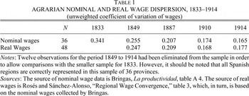
However, analyses of the pattern and extent of migration flows shed little light on the issue of integration. Markets could be perfectly integrated but exhibit scant movements of labor or they could exhibit high rates of movements but be in fact poorly integrated. The explanation of such a paradox is straightforward. When two labor markets are integrated real wage differentials are so small that they do not cover the costs of moving from one region to another. Instead, two poorly integrated labor markets exhibit such huge wage differentials that possible wage gains covered moving costs. Consequently, a more efficient measure of integration is wage differentials. Price gaps and price dispersion should decline whereas price correlation between markets should increase as market integration progresses in factor markets in the same way as we observe in commodity markets. Applying this principle, a simple and widely used measure of market integration is the unweighted coefficient of variation of wages across regions.27
The unweighted coefficient of variation in a particular year is the standard deviation of wages divided by the mean.
provides evidence.
These coefficients of variation of agrarian wages show a significant downward trend exhibiting the typical behavior of convergence processes resulting from market integration. Similar trends are also observed for unskilled urban and industrial workers' wages from 1850 to 1914. We also observe a declining wage gap between urban and rural wages between 1860 and 1914 and find that Spanish wage gaps were smaller than urban-rural wage gaps of other countries such as France, the United States, and Britain.28
Rosés and Sánchez-Alonso, “Regional Wage Convergence,” table 5.
Obviously, all evidence seems to indicate that the Spanish labor market became increasingly integrated in the second half of the century.
29 Note that this conclusion represents a departure from the previous literature. The few historians who have previously examined the Spanish labor market before 1914 were generally struck by its apparent poor performance. These studies leave the strong notion that, even if there was some migration, opportunities for arbitrage were not fully exploited (see, for example, Mikelarena “Los movimientos migratorios”; and Simpson “Real Wages”).
Thus we find that in the prerailway age, the signs of the emergence of a national transportation system were clearly visible as roads and coastal shipping connected regions. Even so, evidence also seems to indicate that transportation costs declined sharply during the first half of the nineteenth century but there is still doubt as to whether the integration of commodity markets was completed before or after railways. Moreover, data show factor markets integrating later than commodity markets during the second half of the century. According to this, one may confidentially assume that the movements of capital and labor across Spanish regions and provinces were by far less important than the movements of goods.
MANUFACTURING LOCATION AND CONCENTRATION
This section examines changes in manufacturing location and concentration simultaneous to the progressive integration of Spanish commodities and factor markets during the nineteenth century. First, it shows that manufacturing location varied across regions during this period. Second, it documents how divergent location trends are mainly caused by changes in the location of modern industries. Third, it also establishes that traditional and modern industries had different concentration levels.
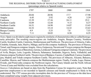
The regional distribution of manufacturing employment varied considerably from the end of the eighteenth century to the early twentieth century. As shown in Table 2, Catalonia and the Basque Country doubled their participation in overall figures. Particularly, the share of Catalonia in manufacturing employment increased from 12 percent in 1797 to about 17 percent in 1860 and over 25 percent in 1910. By contrast, other regions such as Northern Castile and Aragón lost ground remarkably, halving their shares. Andalusia, the most populated region, lost its industrial leadership but retained an important share (about one-fifth) of national manufacturing employment. Finally, other regions such as the Mediterranean, the Northwest, and Southern Castile maintained, with small changes, their relative participation in overall figures.
In accordance with the manufacturing location trends observed in Table 2, the nineteenth century can be divided into two periods: the first half (up to 1860) and the second half (from 1860 to 1910). During the first half of the century, only Catalonia and the Northwest region significantly increased their shares and Aragón and Northern Castile fell behind appreciably. In the second half, Catalonia continued with its expansion but the Basque Country witnessed a rapid increase in its figures. At the same time, the industrial progress of the Northwest regressed and the de-industrialization of Northern Castile intensified. Finally, Andalucia, Aragón, and Southern Castile lost ground slightly whereas the Mediterranean region maintained its share in national totals.
A satisfactory description of changes in manufacturing location must include consideration of the different evolution of traditional and modern industries.30
Chemicals, textiles, metallurgy, and engineering compose the modern industry whereas the rest of manufacturing forms the traditional sector. Although it would be desirable to also include other small industries, such as paper and flour mills, in the modern category, there are no data on regional employment in these industries.
For each of the eight macro-regions,
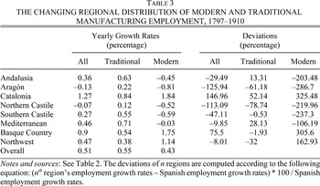
Table 3 not only reports growth rates of manufacturing employment from 1797 to 1910 but differentiates growth rates for both modern and traditional industries. It also presents the percentage deviation of these growth rates from overall Spanish growth rates.
Table 3 reveals that employment growth rates varied widely across regions and traditional and modern industries. In all regions, employment in traditional industries grew from 1797 to 1910 whereas, in sharp contrast, the employment in the modern ones only increased in Catalonia, the Basque Country, and the Northwest. Likewise, the largest deviations from the Spanish average were in the modern industries with extraordinary differences between the two most industrialized regions (Catalonia and the Basque Country) and the rest. Therefore, the evolution of the traditional industries does not contribute much to our understanding of the differences in manufacturing employment growth rates whereas the contrary holds for the dynamics of modern industries. That is, the changes in the regional distribution of the manufacturing employment can be mainly attributed to changes in the sphere of modern industries.
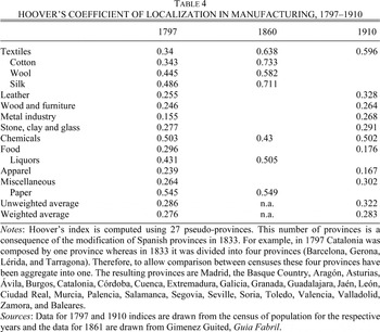
It seems plausible to suppose that there was also a modification of the level of geographic concentration associated to this dramatic change in the location of industries. A simple and common way of finding changes in geographic concentration of industries is to estimate Hoover's coefficients of localization.31
To compute Hoover's coefficient first estimate the following location quotient (LOij)
where Lij is employment in industry i, for province j, Lj is the total industrial employment for province j, and LiSp is employment in industry i, and LSpis total employment in Spain. Then place the provinces in decreasing order by their location quotients, and compute the cumulative percentage of employment in industry i over the provinces (y-axis). Finally, compute the cumulative percentage of employment in total manufacturing over the regions (x-axis).
This is similar to the Gini coefficient and, hence, it should be interpreted similarly. If the coefficient is equal to zero, the industry is completely dispersed across the regions. If it is equal to one, the industry is completely localized in one region. In this case, Hoover's coefficients are calculated using employment for nine pseudo-two digit manufacturing sectors and three benchmark years (1797, 1860, and 1910).
32 The Spanish data are less detailed than today's two-digit SIC data. Nowadays, 20 categories comprise manufacturing standard two-digit SIC data whereas Spanish data only furnish information up to nine categories. Obviously, this data limitation reduces the amount of observed manufacturing concentration. Ellison and Glaeser (“Dartboard Approach,” table 5) showed that raw geographic concentration of industry doubled as one moves to finer industry definitions (for example from two-digit to three-digit SIC definition; that is, doubling the number of categories). Consequently, one can confidentially predict that the “real” Hoover's coefficient at two-digit SIC is about one-and-a-half times or twice as big as the observed.
The unweighted and weighted averages of Hoover's coefficient indicate that manufacturing became slightly more concentrated during the nineteenth century (see Table 4). An important element in this trend was a pair of industries (apparel and food) that became relatively more regionally dispersed and important in terms of employment over time. Therefore, the aggregate coefficient hides the notable tendency towards the concentration of several industries. Specifically, textile, metal, miscellaneous, and leather industries became more regionally localized throughout the entire period. Instead, other industries, such as chemicals, stone, clay and glass, and wood and furniture, exhibited little change in location during this period. Note that the two leading sectors of industrialization (metal and textiles) were among those industries increasing their concentration levels. In the case of textiles, concentration appears to have been especially strong between 1797 and 1860 during the early phases of the transition from cottage to factory production, and the early phases of market integration.
EXPLAINING REGIONAL SPECIALIZATION
As a large literature has emphasized, regional specialization may arise as regions make use of their comparative advantage, benefit from increasing returns in production, or both. We can illustrate this by assuming that, under autarky, each region produces all the goods that it consumes, the location of industries is stable and the level of industrial concentration is low. When trade costs decrease and product markets tend to integrate, the HO model predicts that regional specialization will arise as regions produce and export products that are relatively intensive in their abundant resource.33
See Flam and Flanders, Heckscher-Ohlin, for a presentation of the theory. See also O'Rourke and Williamson, Globalization, for an application of the HO framework to history.
Consequently, it holds that specialization occurs to take advantage of intrinsic diversity.
34 It should also be noted that the HO model predicts convergence in per capita income across regions that, unfortunately, does not conform to Spanish history during the nineteenth century. This result is motivated by the factor-price-equalization (FPE) theorem, a core result of the HO model. This theorem states that in equilibrium, given a variety of restrictive assumptions, factor prices will be equal across regions. Clearly such perfect outcomes are not observed in the real world but trade economists generally accept a looser version of this theorem, arguing that commodity-price convergence induces factor-price and real-income convergence. See, for example, Leamer “Heckscher-Ohlin Model.”
In other words, regions differ in their factor endowments and these differences establish comparative advantages, interregional trade, and, hence, regional specialization. Regions with a small population and an abundant supply of land will produce goods that require large areas of land but are not intensive in labor. On the other hand, regions well endowed with labor but relatively scarce in land will specialize in manufactured goods that are intensive in labor. Exports from one region to the other will be largely based on goods that are intensive in those factors of production with which they are abundantly endowed and the prices of which are therefore low.
35 Flam and Flanders, Heckscher-Ohlin, p. 90.
The new economic geography has introduced an increasing-returns (IRS) model that concludes that industrial concentration arises to take advantage of scale and variety gains from specialization.36
See, for example, Krugman, “Scale Economies,” Geography, and “Increasing Returns”; Krugman and Venables, “Globalization”; and Fujita, Krugman, and Venables, Spatial Economy. Moreover, the IRS model appears to reconcile with Spanish history during the nineteenth century because it predicts manufacturing concentration and income divergence with market openness.
Consequently, it conjectures that regional specialization will take place if external economies are substantial or if economies of scale determine that only a few large plants can satisfy total demand more efficiently. Moreover, as Paul Krugman indicates, in this situation the size of local (idiosyncratic) demand is what decides the location of the industries producing differentiated goods.
37 Instead, in a situation with zero transportation costs and identical and homothetical tastes, and hence decreasing returns, strong domestic demand for a good will tend to make it an import rather than an export (Krugman, “Scale Economies,” p. 955).
There are two major explanations why local demand turns out to be important for industrial location. One is directly related to the pure effect of market size. Due to economies of scale, each differentiated good is produced in only one place, and put on the market in both. If the cost of production is equal on both sites, then the deciding factor in localization is transportation costs because, obviously, total transportation costs are lower if production takes place in the region with the larger market.
38 Inversely, if transportation costs are high or if the markets of both regions are the same size, full concentration of the increasing-returns industry in the larger region will no longer take place. See Helpman and Krugman, Foreign Trade, for a powerful development of this theory and, also, Davis “Home Market,” for a severe criticism on its assumptions.
A straightforward extension of this is that, with market integration, small countries or regions will lose a large part of their industry.
39 This is the so-called Linder hypothesis (see Linder, Trade).
The second explanation points out that location advantage based on market size may arise if there are sufficiently strong backward and forward linkages (externalities), which in turn generate increasing returns in the production of intermediate inputs.
40 Krugman and Venables, “Globalization.”
Alfred Marshall was the first to introduce the concept of external economies and also identified up to three different reasons why the co-location of industries might generate externalities. First, a geographically concentrated industry could maintain a large group of specialized local suppliers of inputs saving transportation and transaction costs. Second, it could also generate more efficient labor markets because specialized workers in a certain industry would be less likely to remain unemployed when there were a large set of plants of the same industry co-located. Likewise, firms would be more likely to find specialized labor when they needed it. This promotes skilled labor. Finally, the proximity of firms would make the spread of information and, hence, the rapid diffusion of technology and innovations easy.
41 There is a large literature on this issue. See, among others, Marshall, Principles; Pred, Spatial Dynamics; and Henderson, Urban Development.
Roughly, a simple version of IRS model operates as follows. When transportation costs are high, there is little interregional trade and regional specialization. In other words, manufacturing establishments are not concentrated as all regions consume and produce all variety of goods. Local wages depend mainly on the size of the regional workforce and will decrease when the number of workers in the region increases. When transportation costs decrease, interregional trade increases.42
Note that in HO and IRS models the force driving regional specialization is a reduction in trade costs (see, for example, Krugman and Venables, “Globalization”), whereas the integration of markets is not a necessary condition for increasing regional specialization.
The typical firm sells extensively in all markets but it preferably establishes itself in the region with larger markets, so it can serve a large local market at low transportation cost. Manufacturing plants concentrate in the regions with higher demand, while all other regions suffer de-industrialization.
43 Nevertheless, if economic integration is characterized by greater mobility of labor and capital relative to that of commodities, then the outcomes of the IRS model vary substantially (see, for example, Krugman and Venables, “Globalization”; and Fujita, Krugman and Venables, Spatial Economy). Thus, with decreasing transportation costs and growing migration rates, the model predicts three different outcomes. An initial period of wage and income per capita convergence with population moving to the region offering higher wages. In the following stage, there will be a new equilibrium with equal wages across regions and with workers evenly divided. The model also predicts a third period characterized by increasing wage (and income) divergence with workers concentrated in the regions offering the higher wages.
Consequently, a regional division of labor spontaneously arises through a process of uneven development.
Recently, Donald Davis and David Weinstein have explored the power of HO and IRS models to account for the location of manufacturing production in a series of papers.
44 See Davis and Weinstein “Market Access” and “Economic Geography”; and Davis, Weinstein, Bradford and Shimpo “Factor Abundance Theory.”
It is one of the characteristics of their work that they use a framework that nests an IRS model within an HO model. So they have build a straightforward model in which specialization in industries is driven by factor endowments and increasing returns lead to intra-industry specialization, that is, determine the output of goods within industries.
45 Davis and Weinstein (“Market Access,” pp. 14–15) give the following definition of goods and industries: “Under the hypothesis of increasing returns, a good is a collection of a large number of varieties produced under monopolistic competition … By contrast, under the hypothesis of comparative advantage, a good is a traditional homogeneous commodity. Industries, in both frameworks, consist of a collection of goods produced using a common technology.”
In other words, the endowments (HO model) determine the broad industrial structure by regions (e.g., if it produces textiles or machinery), but they tell us nothing about the composition of production across the goods within an industry (e.g., if it produce cotton or wool textiles), which is decided by IRS forces. To identify the presence of these IRS effects, they performed an econometric test based on a simple insight derived from the seminal ideas of Paul Krugman: in a world of comparative advantage, unusually strong demand for a good will tend to make it an import, ceteris paribus, whereas in a world of economic geography, this will tend to make it an export. More formally, according to their framework, the output,
X, of the good
g in industry
n in region (province)
p is given by
46 See Davis and Weinstein (“Economic Geography”) for a more detailed discussion of the mathematics.
where Ωgn Vpis the endowments effect and Idiosyncratic Demand is the economic-geography effect. More specifically, Ωgn is the inverse of the technology matrix mapping output into factors, Vp is the vector of endowments of province p, and the idiosyncratic demand is computed as
where D denotes absorption in province P or the rest of Spain, RSP.
47 It should be noted that this equation simplifies the geography implicit in Krugman (“Scale Economies”) and, hence, does not consider demand in adjacent regions.
In other words, local demand is not measured as a total aggregate for each region but as the demand deviation (idiosyncratic demand) for a good in a region relative to the sum of all other regions. As noted previously, the key to establishing the presence of IRS effects is the coefficient of the
Idiosyncratic Demand variable, for which Donald Davis and David Weinstein identify three hypotheses. In a comparative advantage world without transaction costs, where factor endowments suffice to decide production, the localization of demand should have no effect on production structure, so it would no be different from zero. Instead, in a world with both friction and comparative advantage, the geographical localization of demand becomes all the more relevant, so the coefficient would be positive and greater than zero. In this situation two cases are possible. If this coefficient lies between zero and one, we are in a comparative advantage world with transaction costs. Instead, if it is greater than one, we are in the IRS case, where the response of local producers to idiosyncratic components of demand is more than one-to-one.
THE LOCALIZATION OF PRODUCTION
Before proceeding with the direct estimation of the main model (equation 1), it appears useful to investigate the impact of HO framework on the localization of the production across Spanish provinces. So I compute several regressions using production as the dependent variable and endowments as independent variables. In other words, I estimate the following linear relationship
48 See Davis and Weinstein (“Economic Geography”) for the assumptions of this estimation.
where the output, X, of industry n in region (province) p is a linear function of the Σn, the inverse of the technology matrix mapping output into factors, and Vp, the vector of endowments of province p.
The econometric analysis is performed with 1861 manufacturing output data and 1859–1860 data for all right-side variables (endowments) in order to avoid simultaneity problems.49
This is the “classical” procedure in the literature.
There are good reasons to prefer mid-nineteenth-century data to investigate the determinants of manufacturing location in Spain during industrialization. First, as shown in the section on regional specialization, the process of re-location and manufacturing concentration was at work by the mid-nineteenth century. Second, a rapid decrease in conventional transportation costs had happened over the previous 30 years.
50 Moreover, it is likely that the estimation of the HO model in alternative years at the beginning or at the end of the nineteenth century might offer less conclusive results. At the beginning of the nineteenth century, market integration forces had just recently become active and at the end of the nineteenth century large movements of production factors took place across Spanish provinces.
And, finally, manufacturing data for 1861 are of extraordinary quality.
The data used for the analysis include manufacturing output, endowments, and technology for 43 of 49 provinces in Spain.51
This article takes provinces in Spain as the geographic unit of analysis. Spanish provinces are mid-sized because they are bigger than French departments or British counties, but smaller than U.S. states. It should be noted that the definition of Spanish provinces in 1833 was not based on geographic criteria but rather the Spanish government created provinces following pre-existing historical divisions and the areas of influence of major towns. For that reason, Spanish provinces adjust quite well to the functional integration principle that defines regions by the presence of a nucleus and the corresponding area of influence. If one wants to estimate an IRS model, the unit-of-analysis should be defined in such a way. Instead, these kinds of analysis units pose problems in quantifying the HO framework, where factors should be mobile within regions but less so across regions (see, Kim, “Expansion,” p. 884, for a discussion of the question).
Six provinces (Alava, Canary Islands, Guipúzcoa, Navarra, Orense, and Vizcaya) have been eliminated from the sample due to the incompleteness of their data. This implies that the Basque Country is excluded from the regressions. Factor endowments considered are capital, land, professions, artisans, unskilled, and agrarian labor.
52 In empirical literature, some authors employed education-based classifications of labor whereas others preferred occupational-based classifications (see, for example, Trefler, “Missing Trade”) but occupational-based classifications are likely to be less exogenous with respect to output shares than are occupational classifications. However, in this case, occupational-based classifications are probably preferable to the educational-based classification for two reasons. The first is that the 1860 census did not record education levels, but literacy. Second, as a large literature has pointed out, literacy is a very poor proxy for skills in the mid-nineteenth century.
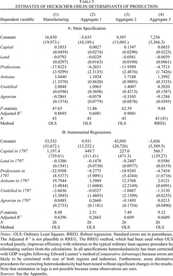
There are, however, two major drawbacks that need to be addressed before proceeding further. According to the literature, differences in technology across industries should be taken into account and endowments do not matter at the finer levels of aggregation. Consequently, the HO framework is estimated for the whole manufacturing sector and separately for three different subaggregates, which pooled several manufacturing sectors (Table 5, panel A). To combine different sectors, the aggregation criteria is the capital-labor ratio.53
The source for capital-labor intensity ratios is Gimenez Guited, Guia fabril.
The resulting aggregates are: the metal industry, cotton spinning, wool spinning, silk spinning, and paper (aggregate 1); flour mills, textiles, and leather (aggregate 2); and olive oil refining, liquor distilling, and soap and cork manufacturing (aggregate 3).
54 The (weaving and finishing) textile industry had significantly smaller capital-labor ratios than did cotton, wool, and silk spinning because it was less mechanized. Consequently, I decided to separate textiles into several industries.
It is also not realistic to assume that the HO determinants of manufacturing location (that is, endowments) were completely exogenous to manufacturing production. Regions with more manufacturing attracted unskilled workers because labor demand was growing and wages were higher during their early industrialization. Similarly, the agrarian workforce decreased in these regions because employment opportunities in the manufacturing sector were rising. A solution to this problem requires the identification of exogenous instruments. Any direct measure of endowments is eligible as an instrument if it is not driven by the development of manufacturing. For this reason, obvious candidates as instruments are endowments before early industrialization.55
Spanish historiography agrees that early industrialization in Spain started on the 1830s.
Thus my hypothesis is that the early endowments in Spain did not reflect movements of factors that were driven by industrialization forces but did have a lasting influence on mid-nineteenth-century manufacturing location. For that reason, I compute another set of regressions using manufacturing production in 1860 as the dependent variable and endowments in 1797 as independent variables (
Table 5, panel B).
Table 5, panel A reports the results of the main specification, regressing 1861 manufacturing output on 1859–1860 endowments. They are both significant and plausible. The adjusted R2 and F-statistic are relatively high in manufacturing and aggregates 1 and 2, but not in aggregate 3. This suggests that even after controlling for size-based variation; endowments explain almost the 85 percent of the variance of aggregate manufacturing output. They also explain about the 60 percent in the highest capital-labor ratio industries, which formed aggregate 1, and about 90 percent in the case of the high consumption sectors, which formed aggregate 2. Instead, the HO framework yields little information on the localization of the traditional industries with the lowest capital-labor ratio, which formed aggregate 3. However, these industries are quite reasonable candidates for an explanation based on natural advantage rather than comparative advantage. For example, the olive oil refining industry was surely affected by the suitability of the provinces' climates for growing olives. The sign and coefficients of the different variables also lie within what one can expect. Provinces well endowed with capital, artisans, and unskilled labor had a comparative advantage in manufacturing, whereas the contrary holds for provinces well endowed in land, agrarian labor, and professions.
In panel B of Table 5, I regress 1861 manufacturing output on 1797 endowments.56
Caution is required in interpreting the result presented in panel B. It should be noted that the regressions suffer from few degrees-of-freedom (the reasons for this is discussed in the notes to Table 4) and, hence, the adjusted R2 and F-statistic are large by construction. Furthermore, estimates of endowments in 1797 are likely to be error ridden. Nevertheless, the major effect of measurement error would be to create an attenuation bias toward zero. Therefore, one might presume that the coefficients obtained are, if anything, underestimates.
The results are not identical to those in panel A, although they are similar. In all specifications I find that provinces relatively abundant in artisans and capital and relatively scarce in professions and land in 1797 were substantially more industrialized by 1861.
57 Note that the coefficient of capital is only significant in aggregate 3.
Instead, the coefficients of agrarian and unskilled labor had the wrong sign or are not significant. This intriguing result is consistent with the possibility, discussed earlier, of reallocation of production factors as a consequence of early industrialization during the first half of the nineteenth century. Therefore, it seems that early industrialization in Spain reallocated workers from agriculture to industry and from agrarian to industrializing provinces.
58 Given the long span of time (60 years) considered here, this reallocation would be produced not only by reallocations of labor across sectors and provinces but also by differences in life expectancy and birth rates across provinces. In this sense, it is well known that in industrializing regions birth rates were higher (due to earlier marriages) and mortality rates were also higher (due to poor hygienic conditions in industrial districts and working conditions).
Instead, one can confidentially suppose that the movements of artisans, professions, capital and, obviously, land across provinces and sectors were less important.
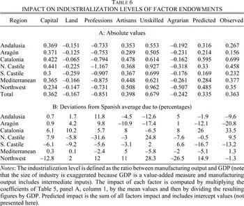
For seven of eight macro-regions (the Basque Country is excluded due to data incompleteness), Table 6 reports the impact of factor endowments on industrialization levels, employing the main specification. To assist interpretation, the last two columns of the table indicate, respectively, the predicted and the observed industrialization levels and panel B the deviations from the Spanish norm. Regions such as the Mediterranean and Andalusia have industrialization levels quite similar to that of Spain as a whole, and for them the exercise furnishes little information. The regions with industrialization levels far above or below the national are of course of most interest.
What is remarkable in this simulation is the fact that a large part of variation in regional industrialization levels still remains unexplained after taking into account endowments. As the last two columns of Table 6 show, differences between predicted and observed values at regional level are large and significant. To give an example, endowments predict a 37 percent higher level of industrialization in Aragón than the observed level. Consequently, the estimates of the HO model do not necessarily reject an interpretation of the differences in regional industrialization levels based on economic geography forces.
Despite these major reservations, the exercise in Table 6 can also be employed to suggest endowment-based interpretations of the divergent evolution of industrialization in Spanish regions. It reveals that Andalusia was relatively poorly endowed in unskilled and artisan labor. Catalonia had a relatively high industrialization level due to the relatively scarcity of land, professions, and agrarian labor and the relative abundance of artisans and capital. Instead, unskilled labor was a minor player in explaining the Catalan exceptionality. In a sharp contrast with Catalonia, the lower industrialization levels of Northern Castile are largely explained by the abundance of land, agrarian labor, and professions. In the case of Southern Castile, capital also played a role in lowering industrialization levels. In the Mediterranean region, unskilled labor was too scarce and agrarian labor and professions too abundant. Finally, the evolution of the Northwest can be explained by appealing to its capital scarcity and abundance of agrarian labor.
ECONOMIC-GEOGRAPHY EFFECTS IN SPANISH MANUFACTURING
There were significant economic-geography effects in Spanish manufacturing by 1861. To compute these effects I estimated equation 1 following Davis and Weinstein's methodology. This equation can be estimated at various levels of aggregation, as linear specification or as a system of seemingly unrelated regressions (SUR).
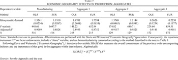
Table 7 reports estimates of full equation 1 at higher levels of aggregation. What is striking in these estimates is the fact that the regressions fits are quite high. Indeed, it shows that at the end of the early phase of Spanish industrialization, factor endowments with economic geography specifications explained about the 90 percent of the variation in these aggregates. The results also bolster our confidence in the economic-geography effects. Idiosyncratic demand is significantly larger than one in three of the four aggregates computed, whereas it is close to zero only in one (aggregate 3), which corresponds to traditional industries where natural advantages were very important.
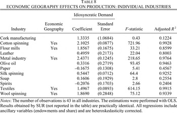
One could run an additional robustness check to confirm that the regression is identifying economic-geography effects. The results are obviously very sensitive to the aggregation scheme. For example, combining industries with constant returns with industries with increasing returns might dilute the real effects. One simple solution to that problem is to compute equation 1 in full for each industry individually. Table 8 shows the results for that exercise.
The economic-geography effects are significantly larger than unity for five of 12 sectors: cotton spinning, flour mills, the metals industry, textiles, and wool spinning. Furthermore, the results are robust to whichever method of estimation one chooses.59
The β-coefficients of Idiosyncratic Demand (not reported in the table) for these five industries also show very statistically significant economic-geography effects. They are typically over the 0.8 range (3.45 for flour mills, 0.91 for cotton spinning, 0.84 for the metals industry, 0.81 for textiles, and 0.81 in wool spinning). A one-standard-deviation movement in idiosyncratic demand on average moves production by more than 0.8 standard deviation. In other words, observed fluctuations in idiosyncratic demand provide a lot of information on production patterns.
Moreover, perhaps with the exception of flour mills, all of the industries with significant economic-geography effects seem plausible candidates for monopolistic competition. For example, Paul Krugman identified the metal industry and textiles as classical examples of industries where backward and forward linkages are important.
60 It is also interesting to note the similarity of my estimates with Donald Davis and David Weinstein's estimates for Japan and the OECD countries.
61 Davis and Weinstein, “Market Access” and “Economic Geography.”
They obtained significant economic-geography effects in about 42 percent of Japanese industries and in about 34 percent of OECD industries, whereas my exercise obtains this result in about 42 percent of the cases.
The 12 sectors in Table 8 corresponded to about the 82 percent of value added in industry by 1861.62
Using the value-added shares computed by Prados de la Escosura, De Imperio, pp. 143–67.
Moreover, the sectors with economic-geography effects account for 55 percent of the value added in industry by 1861. This obviously strengthens the view that the sectors that seem to have home- market effects account for the major part of industrial output in Spain during early industrialization.
CONCLUSIONS
This article offers new insights concerning the causes of the industrialization of Spain's regions by applying recent development in international economics. The fortunes of a region are assumed to depend not only upon its own endowments but also on market-size effects. By contrast, many economic historians take a different approach assuming that the fortunes of each region has their own specific explanation. From the previous pages, a common pattern emerges: regions industrialized or failed to do so according to a combination of comparative advantage (HO model) and IRS forces.
It seems necessary to emphasize that endowments are not enough to explain the full history. Why did modern manufacturing concentrate in some regions while others, in spite of their comparative advantage in manufacturing, have few modern factories? The explanation lies in the fact that modern industries that produced heterogeneous goods exercised monopolistic competition and experienced increasing returns. Consequently, they tended to be concentrated in regions in which the home-market effects were larger.
What really caused these home-market effects? It is premature to attempt to answer this here, but a few hypotheses might be ventured. Home-market effects can arise from simple market-size scale economies or the much more sophisticated Marshallian externalities (backward and forward linkages). Many manufacturing sectors with increasing returns are also sectors with backward and forward linkages. Consequently, it is much more plausible that Marshallian externalities were more important for producing home- market effects than pure market-size effects. In any case, these are simple observations that require much greater analysis and empirical study.
These findings suggest the appeal of some sort of evolutionary interpretation of the changes in the location of the Spanish manufacturing during the nineteenth century. In the eighteenth century, due to high transportation and transaction costs, there was little interregional trade and regional specialization was scarce. In the first half of the nineteenth century, transportation and transaction costs decreased. Trade among regions increased and regional goods markets became steadily more integrated. At this point, manufacturing location varied. These changes in the location of manufacturing production arose both from comparative advantage and from additional external economies. Increasing returns were highly relevant in the new modern manufacturing industries, which produced heterogeneous goods, but negligible in traditional industries. Some regions with a large comparative advantage in manufacturing because they were well endowed in artisans and capital, such as Catalonia, also benefited from gains from external economies. The production structures of Agrarian (poor) regions did not converge with those of industrialized regions for two reasons. First, increasing-returns industries did not move into poor regions. Second, agrarian labor did not migrate massively to the new rich regions up to the first third of the twentieth century.
Finally, I would like to underline three broad suggestions for further research. First, the article's findings suggest the need for rethinking the relationship between agricultural revolution and regional industrialization. I believe that the conventional view of successful industrialization as exclusively determined by the success of a previous agricultural revolution is too simple. With the results obtained here, it seems much more productive to study the relationship between agricultural changes and regional differences in factor endowments. Second, it also appears necessary to study the forces shaping the regional distribution of endowments and particularly the influence of pre-industrial institutions on that distribution. Third, from the point of view of economic theory, this article has supplemented the explanatory power of the new economic geography in economic history. In particular, the hypothesis of the importance of home-market effects in determining the localization of production is fully confirmed by this research.
Appendix: Description of the Variables and Their Sources
This Appendix describes chronologically the process of construction and the sources of the different variables used in the calculations.
Provincial-level data on sectoral output of 16 manufacturing sectors in 1861 were taken from Gimenez Guited's book.63
Gimenez Guited, Guía Fabril.
In calculations, I have employed a concept closely allied to gross output: gross output less intra-industry transactions.
64 See, Ciccone and Hall (“Productivity,” p. 60) for a detailed discussion of the advantages of that output concept in regional studies.
1859–1860 data have been used to compute endowments and other right-hand-side variables. The numbers of different categories of labor by provinces were taken directly from the Population Census of 1860 and then added to get labor-category totals: professions (clerks, public servants, professionals, and commerce), artisans, unskilled (day workers, construction workers, transportation workers, miners, poor, servants, and factory workers), and agrarian labor.
Two different methods can be employed to compute capital endowments by province. First, the data on housing prices, as a proxy for capital prices, from the property provincial bureaus can be used directly (capital 1).65
The data include the prices and quantities of houses sold during the year, the prices and quantities of houses transferred by inheritance, and the prices and quantities of houses that were settled in mortgage. Specifically, in the calculations, an average of these three prices during two years (1863–1864) has been employed. Finally, average prices per house were transformed in prices by m2with data on the average size of houses by province from 1874 statistics. All data were taken directly from Ministerio de Gracia y Justicia, Estadísticas.
Alternatively, the capital stocks by province can be derived from income taxes in 1860 (
capital 2). Spain's statistical yearbook gives taxes paid by rents of housing, agrarian equipment, livestock, commerce, and industry for each province in 1860.
66 Anuario estadístico de España.
These taxes were used to assign capital rents for each province and kind of capital good in 1860 using tax rates. Capital rents were used to estimate capital stock levels using the interest rate (6 percent), provincial-capital-goods price deflators, and rates of depreciation,
67 This estimation is derived from the following identity the StockK=(RentK)/(I+δ) where I is the interest rate and δ is the depreciation rate.
which were different for each kind of capital good.
68 The provincial deflators for housing and livestock were taken from Rosés and Sánchez-Alonso, “Wage Convergence.”
In the regressions, these two variables are significant and have the expected sign (negative in
capital 1 and positive in
capital 2) but in the tables I preferred to show
capital 2 given that it corresponds quite well with the variable employed by Davis and Weinstein.
The next problem was how to estimate land endowments by provinces. Several alternatives were available. First, average land prices can be directly employed (land 1).69
I use the same source and methodology as in the case of housing prices.
Secondly, I can use the quantity of hectares of cropland and pastures from the first available and reliable census (
land 2).
70 Banco Urquijo, La riqueza, vol 2, p. 378.
Third, I use government estimations on land rents to estimate land values (
land 3). Spain's statistical yearbook provides information on the amount of provincial land rents.
71 Anuario estadístico de España.
These rents were used to compute land stocks for each province in 1860, using the interest rate (6 percent) and provincial land deflators. Fourth, given that some scholars have expressed doubts on the reliability of land taxes, I modify the original data on the amount of provincial land rents with estimations on the amount of tax evasion by province (
land 4).
72 Pro Ruíz, “Ocultación,” p. 93.
In regressions, all alternative variables were significant and displayed the expected sign. In the tables, I preferred to show the variable
land 3 because it is the most satisfactory from the theoretical point of view.
A proxy for the provincial Gross Domestic Product in the private sector was estimated for all provinces in the sample. This variable was exclusively used to weight the regressions in order to correct for heteroskedasticity. The provincial GDP was computed by adding up land, housing and other capital rents, depreciation, and wages (including the remuneration of the self-employed). Complete provincial data on unskilled wages was combined with data on the size of the workforce and skill premiums by categories of workers to get employee remuneration.73
The data for unskilled wages came from Rosés and Sánchez-Alonso, “Wage Convergence”; and the data on skills premium came from U.S. Congress, Labor, pp. 1345–441.
Moreover, the remuneration of self-employed labor was assumed to be equal to the remuneration of skilled labor. Land, livestock, and capital rents were computed from taxes paid on land, livestock, and industry and commerce, respectively.
74 Anuario estadístico de España.
Depreciation rates for each type of good were also imputed from contemporary references. All provincial figures were increased so that the 49-provinces total for GDP exactly matched the total Spanish GDP of the private sector.
75 Data on Spanish GDP are from Prados de la Escosura, El progreso.
A PPP-adjusted price index deflated the resulting current GDP figures.
76 The deflator came from Rosés and Sánchez-Alonso, “Wage Convergence.”
1797 data have been used to compute endowments in instrumental regressions (Table 5, panel B). The numbers of different categories of labor were introduced by provinces directly from the Population Census of 1797 and then added to get labor-category totals. Given the absence of estimates on capital, urbanization rates (cities with more than 5,000 habitants) were used as a proxy. Finally, as a proxy for land values, agrarian production from the Censo de la Riqueza Territorial e Industrial was used.
The construction of the consumption data by province was quite complex. In broad terms, three types of consumption goods were used in this study: intermediate (cotton yarn, wool yarn, silk yarn, and metal goods), taxed goods (olive oil, liquors, cork, paper, and soap), and duty-free goods (flour, leather, and textiles). The consumption of intermediate goods for each province was computed using Gimenez Guited's data.77
Gimenez Guited, Guia Fabril.
However, in the absence of direct figures on the provincial consumption of metal goods, their consumption was imputed from the figures on machinery stocks by province. For taxed goods, Spain's statistical yearbook provides the quantities consumed by each province's capital.
78 Anuario estadístico de España.
Then, provincial totals were computed under the assumption that provincial per capita consumption of each good corresponded to the pattern of its respective capital. Finally, provincial data on household consumption, which broke household consumption into several categories, provided the basis of figures for the provincial consumption of flour, leather, paper, and textiles.
79 Rosés and Sánchez-Alonso, “Wage Convergence,” furnishes that data on provincial household consumption.
It should be noted that all these commodities (intermediate, taxed, and duty-free) were valued at producer prices because without this adjustment the data would have greatly overestimated final consumption of goods, given that consumer prices included transportation costs and mark-ups. Finally, all provincial figures were increased so that the 49-province totals for each commodity exactly matched its total Spanish consumption.
80 Data on Spanish consumption are from Prados de la Escosura, El progreso.
I have benefited from the comments of Stefano Battilossi, Klaus Demset, Stefan Houpt, Leandro Prados de la Escosura, Teresa Sanchís, James Simpson, seminar participants at Universidad Carlos III, Universidad Complutense, Fourth World Cliometrics Conference held in Montreal, two anonymous referees, and the editors of this Journal. I gratefully acknowledge the generous permission of Professor Juan Carmona to allow me to draw on our unpublished joint work on Spanish land and housing prices for this article. The Spanish Ministry of Education (Grant SEC 2002-01595) supports this research. The usual disclaimer applies.