1. Introduction
The stability and saturation of resistive magneto-hydrodynamic (MHD) modes are of great importance to magnetic confinement systems such as tokamaks or reversed field pinches (RFP). In an RFP, the plasma is always turbulent due to the continuous interaction of various tearing modes and resistive interchange modes (Bodin Reference Bodin1990). In tokamaks, tearing modes and resistive kink modes may arise from unfavourable current density profiles which drive reconnection at corresponding resonant surfaces, resulting in the formation of magnetic islands which tend to cause confinement degradation (Chang & Callen Reference Chang and Callen1990). Moreover, if left uncontrolled, nonlinearly unstable resistive kinks (Jiang et al. Reference Jiang, Hu, Wang, Shi, Xu, Chen, Ding, Zhong, Dong and Ji2015) or thermally unstable tearing modes (Gates & Delgato-Aparicio Reference Gates and Delgato-Aparicio2012; White, Gates & Brennan Reference White, Gates and Brennan2015) may grow to a large amplitude and trigger disruption. Thus it is of utmost importance to have a thorough understanding of the stability of resistive modes in both the linear and nonlinear phases.
Various methods have been used to study this subject for decades, the most prevalent of which is asymptotic matching. In the outer region, far away from the resonant surface, the ideal MHD equation is solved with the inertial term and dissipation term neglected (Newcomb Reference Newcomb1960; Freidberg Reference Freidberg1987) as they are small compared to the requirement of force balance. This outer solution will produce a singularity near the resonant surface, which must be resolved by considering a scaled inner region near said surface where inertia and dissipation are important (Coppi, Greene & Johnson Reference Coppi, Greene and Johnson1966; Glasser, Greene & Johnson Reference Glasser, Greene and Johnson1975). The outer region and inner region solutions then must match at the boundary between them. The matching of those solutions will yield the eigenvalue for the resistive equation, which is just the linear growth rate. Later, the asymptotic method was also used on a finite size island to determine the mode saturation level in the nonlinear phase (White et al. Reference White, Monticello, Rosenbluth and Waddell1977; Escande & Ottaviani Reference Escande and Ottaviani2004; Hastie, Militello & Procelli Reference Hastie, Militello and Procelli2005).
Although this tried and tested matching method has faithfully served the community for many decades (Furth, Rutherford & Selberg Reference Furth, Rutherford and Selberg1973; Pletzer & Dewar Reference Pletzer and Dewar1991; Chu et al.
Reference Chu, Dewar, Greene and Pletzer1993; Hegna & Callen Reference Hegna and Callen1994; Iacono et al.
Reference Iacono, Bhattacharjee, Ronchi, Greene and Hughes1994), there are some severe limitations in its application. For the zero
 ${\it\beta}$
case, the ideal MHD equation (or the Newcomb equation) has a first-order singularity near resonance, and it has a small solution for the perturbed vector potential
 $u_{1}\sim x$
and a large solution
 $u_{2}\sim 1+x\text{ln}|x|$
. Approaching the resonant surface, the small solution vanishes, while the large solution remains finite. The ratio between the small solution and the large solution is essential in matching the outer and the inner region solutions. This ratio is difficult to calculate numerically due to finite accuracy (Tokuda & Watanabe Reference Tokuda and Watanabe1999) and requires a finite magnetic shear near the resonant surface to be managable.
Things are worse when a finite
 ${\it\beta}$
effect is considered, as it introduces a second-order singularity and the form of the small and large solutions becomes
 $u_{1}\sim x|x|^{{\it\nu}}$
and
 $u_{2}\sim |x|^{-{\it\nu}}$
. The exponent
 ${\it\nu}$
is related to the well-known Suydam–Mercier index, which is a function of pressure gradient and magnetic shear (Suydam Reference Suydam1958; Mercier Reference Mercier1962). As
 ${\it\nu}$
increases, the large solution will be increasingly dominant over the small solution, resulting in increased difficulties when tracking the behaviour of both solutions. First, tracking the two solutions requires increasingly complicated polynomials. The second and more fundamental difficulty is that the asymptotic matching at high
 ${\it\nu}$
requires higher derivatives of equilibrium profiles which are not available in practice. What is more, the difference between
 $u_{1}$
and
 $u_{2}$
could be large to the extent that even the current density within the tearing layer will be hardly affected by discontinuity in the small solution. This makes the meaning of matching the solutions at the boundary layer doubtful.
Further still, when dealing with island saturation, the asymptotic method considers the modified current density profile near the island region, and finds the saturation width by matching the linear solutions for a modified current density profile (Hastie et al. Reference Hastie, Militello and Procelli2005). The method presented here takes one step further, and fully accounts for the effect of the perturbed current by solving the Grad–Shafranov equation within the island region.
In light of the aforementioned difficulties associated with the traditional asymptotic matching technique, an alternative method is used in this paper to investigate the stability and saturation of the resistive mode with finite
 ${\it\beta}$
. This new method rests on the idea that solving the ideal MHD equation is equivalent to solving the Grad–Shafranov equation, thus the ideal mode structure can be obtained as a perturbed equilibrium in both linear and nonlinear cases. In the linear case, the linear growth rate can be found by solving the resistive eigen-equation without the scaled inner region once the mode is found to be unstable from the ideal solution. In the nonlinear case, a finite size island will flatten any equilibrium profile, and eliminate the aforementioned singularities. The saturation size of the island is then determined by the condition that there is no jump in the radial gradient of this perturbed equilibrium helical flux across the resonant surface. Apart from looking for the island saturation level, we will also investigate the critical island size beyond which the Glasser effect vanishes. This finite pressure effect was first described by Glasser et al. (Reference Glasser, Greene and Johnson1975) for the linear resistive mode, then the thin island mitigation of this effect was discussed by Kotschenreuther, Hazeltine & Morrison (Reference Kotschenreuther, Hazeltine and Morrison1985) with the constant
 ${\it\psi}$
approximation. Here, we will present a more careful treatment of perturbed quantities within the island region while solving the Grad–Shafranov equation to find a marginal stable point where the pressure stabilization and current drive balance each other, so that the system is in a de facto equilibrium. It should be noted that this method does not assume
 ${\it\psi}$
within the island to be constant when dealing with island saturation.
The rest of the paper will be arranged as follows. In § 2, the configurations with helical symmetry are described and the equivalence of the perturbed equilibrium and the ideal linear equations are explained. In § 3, a method earlier used by Robinson (Reference Robinson1978) to extract the small and large solutions near the resonance is applied to the case of
 ${\it\beta}=0$
plasma. A special type of current density and pressure profile is constructed in § 4 to allow for the extraction of any high-order terms in the outer solutions near the resonance for
 ${\it\beta}\neq 0$
. Based on this equilibrium, § 5 extends the mathematical method of § 3 to track the high
 ${\it\beta}$
ideal solution behaviour. Further, the origin of the Glasser effect (Glasser et al.
Reference Glasser, Greene and Johnson1975) and the finite island mitigation of it (Kotschenreuther et al.
Reference Kotschenreuther, Hazeltine and Morrison1985) will also be discussed briefly. In § 6, the current and pressure profile modification caused by finite (but still small comparing to system size) island will be described. In § 7, the Grad–Shafranov equation will be solved within the island to find the marginal stable point of the resistive mode, providing a more accurate description for both finite island mitigation of the Glasser effect and nonlinear island saturation. In § 8, discussion regarding inclusion of finite resistivity will be presented. A conclusion is provided in § 9.
2. Perturbed equilibrium and linear MHD equations
In this section, magnetic configurations with helical symmetry are described and equivalence of the ideal linear equation and the perturbed equilibrium outside the resonant surface are outlined. At the same time, the perturbed equilibrium allows for island formation, while the ideal equation leads to the surface currents at the resonant surface, which are not in equilibrium along the surface.
2.1. Cylindrical plasma with a helical symmetry
We consider a cylindrical analogue of a tokamak plasma with large aspect ratio, which is sufficient to give the basic effects of macroscopic MHD instabilities. A magnetic field with helical symmetry
 $k\partial /\partial {\it\theta}+\partial /\partial z=0$
in cylindrical coordinates
 $r,{\it\theta},z$
, where
 $k=n/(mR)$
(
 $m,n$
are poloidal and toroidal wave numbers,
 $R$
is the major radius of an equivalent torus) is described by the following relationships (Zakharov & Shafranov Reference Zakharov and Shafranov1986)
 $$\begin{eqnarray}\displaystyle & \displaystyle B_{r}=\frac{1}{r}{\it\Psi}_{{\it\theta}}^{\prime \ast },\quad B_{{\it\theta}}=\frac{-{\it\Psi}_{r}^{\prime \ast }+kr\bar{F}}{1+k^{2}r^{2}},\quad B_{z}=\frac{\bar{F}+kr{\it\Psi}_{r}^{\prime \ast }}{1+k^{2}r^{2}}, & \displaystyle\end{eqnarray}$$
 $$\begin{eqnarray}\displaystyle & \displaystyle \bar{j}_{r}=\frac{1}{r}\bar{F}_{{\it\theta}}^{\prime },\quad \bar{j}_{{\it\theta}}=\frac{-\bar{F}_{r}^{\prime }+krj_{h}}{1+k^{2}r^{2}},\quad \bar{j}_{z}=\frac{j_{h}+kr\bar{F}_{r}^{\prime }}{1+k^{2}r^{2}}, & \displaystyle\end{eqnarray}$$
 $$\begin{eqnarray}\displaystyle & \displaystyle \frac{1}{r}{\it\Psi}_{{\it\theta}}^{\prime \ast }=B_{r},\quad {\it\Psi}_{r}^{\prime \ast }=krB_{z}-B_{{\it\theta}},\quad \bar{F}\equiv B_{z}+krB_{{\it\theta}},\quad j_{h}\equiv j_{z}+krj_{{\it\theta}}. & \displaystyle\end{eqnarray}$$
Here,
 $\boldsymbol{B}$
,
 $\bar{\boldsymbol{j}}$
are the magnetic field and the current density
 $\bar{\boldsymbol{j}}\equiv {\it\mu}_{0}\boldsymbol{j},{\it\mu}_{0}=0.4{\rm\pi}$
. Without loss of generality, we hereafter assume
 $B_{z}/R=1$
in all cases considered in this paper.
 ${\it\Psi}^{\ast }$
is magnetic flux and current through a helical membrane
 $$\begin{eqnarray}\displaystyle & \displaystyle \boldsymbol{B}^{\ast }\equiv B_{r}\boldsymbol{e}_{r}+(B_{{\it\theta}}-krB_{z})\boldsymbol{e}_{{\it\theta}}=(\boldsymbol{{\rm\nabla}}\bar{{\it\Psi}}^{\ast }\times \boldsymbol{e}_{z}), & \displaystyle\end{eqnarray}$$
 $$\begin{eqnarray}\displaystyle & \displaystyle \boldsymbol{B}=\frac{(\boldsymbol{{\rm\nabla}}{\it\Psi}^{\ast }\times \boldsymbol{h})}{1+k^{2}r^{2}}+\frac{\bar{F}\boldsymbol{h}}{1+k^{2}r^{2}}, & \displaystyle\end{eqnarray}$$
and
 $\bar{F},j_{h}$
are determined by
 $$\begin{eqnarray}\displaystyle & \displaystyle \bar{F}=(\boldsymbol{B}\boldsymbol{\cdot }\boldsymbol{h}),\quad j_{h}=(\bar{\boldsymbol{j}}\boldsymbol{\cdot }\boldsymbol{h}),\quad \boldsymbol{h}\equiv \boldsymbol{e}_{z}+kr\boldsymbol{e}_{{\it\theta}}, & \displaystyle\end{eqnarray}$$
 $$\begin{eqnarray}\displaystyle & \displaystyle \bar{\boldsymbol{j}}^{\ast }\equiv \bar{j}_{r}\boldsymbol{e}_{r}+(\bar{j}_{{\it\theta}}-kr\bar{j}_{z})\boldsymbol{e}_{{\it\theta}}=(\boldsymbol{{\rm\nabla}}\bar{F}\times \boldsymbol{e}_{z}),\quad \bar{\boldsymbol{j}}=\frac{(\boldsymbol{{\rm\nabla}}\bar{F}\times \boldsymbol{h})}{1+k^{2}r^{2}}+\frac{j_{h}\boldsymbol{h}}{1+k^{2}r^{2}}. & \displaystyle\end{eqnarray}$$
Ampere’s law determines
 $\bar{{\it\Psi}}^{\ast }$
in terms of
 $\bar{F},j_{h}$
 $$\begin{eqnarray}\frac{1}{r}\frac{\partial }{\partial r}\frac{r}{1+k^{2}r^{2}}\frac{\partial {\it\Psi}^{\ast }}{\partial r}+\frac{1}{r^{2}}\frac{\partial ^{2}{\it\Psi}^{\ast }}{\partial {\it\theta}^{2}}=-\frac{j_{h}}{1+k^{2}r^{2}}+\frac{2k\bar{F}}{(1+k^{2}r^{2})^{2}}.\end{eqnarray}$$
In equilibrium
 $\bar{F}=\bar{F}(\bar{{\it\Psi}}^{\ast })$
 $$\begin{eqnarray}j_{h}=\bar{F}\bar{F}^{\prime }({\it\Psi}^{\ast })+(1+k^{2}r^{2})\bar{p}^{\prime }({\it\Psi}^{\ast }),\end{eqnarray}$$
where
 $\bar{p}={\it\mu}_{0}p(\bar{{\it\Psi}}^{\ast })$
is the plasma pressure leading to the helical Grad–Shafranov equation
 $$\begin{eqnarray}\frac{1}{r}\frac{\partial }{\partial r}\frac{r}{1+k^{2}r^{2}}\frac{\partial {\it\Psi}^{\ast }}{\partial r}+\frac{1}{r^{2}}\frac{\partial ^{2}{\it\Psi}^{\ast }}{\partial {\it\theta}^{2}}=-\bar{p}^{\prime }({\it\Psi}^{\ast })+\frac{2k\bar{F}}{(1+k^{2}r^{2})^{2}}-\frac{\bar{F}\bar{F}^{\prime }({\it\Psi}^{\ast })}{1+k^{2}r^{2}}.\end{eqnarray}$$
2.2. Perturbed equilibrium
In the long wavelength limit:
 $k^{2}r^{2}\ll 1$
(2.10) can be written as
 $$\begin{eqnarray}\frac{1}{r}\frac{\partial }{\partial r}\left(r\frac{\partial }{\partial r}{\it\Psi}^{\ast }\right)+\frac{1}{r^{2}}\frac{\partial ^{2}}{\partial {\it\theta}^{2}}{\it\Psi}^{\ast }=-(1+k^{2}r^{2})\frac{\text{d}p}{\text{d}{\it\Psi}^{\ast }}+2k\bar{F}-\bar{F}\frac{\text{d}\bar{F}}{\text{d}{\it\Psi}^{\ast }}.\end{eqnarray}$$
It is convenient to introduce the following notation:
 $$\begin{eqnarray}P({\it\Psi}^{\ast })\equiv \frac{\text{d}p}{\text{d}{\it\Psi}^{\ast }},\quad T({\it\Psi}^{\ast })\equiv \frac{1}{2}\frac{\text{d}}{\text{d}{\it\Psi}^{\ast }}(\bar{F})^{2},\quad j_{0}({\it\Psi}_{0}^{\ast }(r))\equiv (1+k^{2}r^{2})P_{0}+T_{0}.\end{eqnarray}$$
So that the unperturbed equilibrium equation can be written as:
 $$\begin{eqnarray}\frac{1}{r}\frac{\partial }{\partial r}\left(r\frac{\partial }{\partial r}{\it\Psi}_{0}^{\ast }\right)+\frac{1}{r^{2}}\frac{\partial ^{2}}{\partial {\it\theta}^{2}}{\it\Psi}_{0}^{\ast }=-j_{0}+2kB_{z},\end{eqnarray}$$
where the subscript ‘0’ indicates the unperturbed quantities:
 $j_{0}=j_{0}(r),P_{0}=P(r),T_{0}=T(r)$
.
We now seek the nearest equilibrium by consider a small perturbation
 ${\it\psi}$
. Let
 ${\it\Psi}^{\ast }={\it\Psi}_{0}^{\ast }(r)+{\it\psi}$
, then the perturbed equilibrium equation is:
 $$\begin{eqnarray}\frac{1}{r}\frac{\partial }{\partial r}\left(r\frac{\partial }{\partial r}{\it\psi}\right)+\frac{1}{r^{2}}\frac{\partial ^{2}}{\partial {\it\theta}^{2}}{\it\psi}=-(1+k^{2}r^{2})\frac{\text{d}P_{0}}{\text{d}{\it\Psi}_{0}^{\ast }}{\it\psi}-\frac{\text{d}T_{0}}{\text{d}{\it\Psi}_{0}^{\ast }}{\it\psi}+2k\frac{\text{d}B_{z}}{\text{d}{\it\Psi}_{0}^{\ast }}{\it\psi},\end{eqnarray}$$
where the last term can be neglected in the strong axial field approximation
 $B_{z}\gg B_{{\it\theta}}$
. Using the relationship between
 $P_{0}$
,
 $T_{0}$
and
 $j_{0}$
, and the long wavelength approximation, we can rewrite (2.14) as
 $$\begin{eqnarray}\frac{1}{r}\frac{\partial }{\partial r}\left(r\frac{\partial }{\partial r}{\it\psi}\right)+\frac{1}{r^{2}}\frac{\partial ^{2}}{\partial {\it\theta}^{2}}{\it\psi}=-\frac{\text{d}j_{z}}{\text{d}{\it\Psi}_{0}^{\ast }}{\it\psi}+k^{2}\frac{\text{d}r^{2}}{\text{d}{\it\Psi}_{0}^{\ast }}\frac{\text{d}p_{0}}{\text{d}{\it\Psi}_{0}^{\ast }}{\it\psi}\end{eqnarray}$$
and further rewrite it in the following form
 $$\begin{eqnarray}\frac{1}{r}\frac{\partial }{\partial r}\left(r\frac{\partial }{\partial r}{\it\psi}\right)+\frac{1}{r^{2}}\frac{\partial ^{2}}{\partial {\it\theta}^{2}}{\it\psi}=\frac{j_{z}^{\prime }}{rF}{\it\psi}+2k^{2}r\frac{p_{0}^{\prime }}{(rF)^{2}}{\it\psi},\end{eqnarray}$$
in order to expose the resonant terms. Here, a resonant function
 $F$
is introduced as
 $$\begin{eqnarray}F\equiv \frac{B_{{\it\theta}}-krB_{z}}{r}.\end{eqnarray}$$
Within its validity at the distance from the resonant surface, the (2.16) is equivalent to the linearized ideal MHD equation. For the purpose of island saturation analysis, it is necessary to use the 2-D version of the current and pressure profiles as
 $$\begin{eqnarray}\displaystyle & \displaystyle \frac{1}{r}\frac{\partial }{\partial r}r\frac{\partial {\it\Psi}^{\ast }}{\partial r}+\frac{1}{r^{2}}\frac{\partial ^{2}{\it\Psi}^{\ast }}{\partial {\it\theta}^{2}}=-j^{\ast }({\it\Psi}^{\ast })+2k\bar{F}-k^{2}(r^{2}-r_{s}^{2})P({\it\Psi}^{\ast }), & \displaystyle\end{eqnarray}$$
 $$\begin{eqnarray}\displaystyle & \displaystyle j^{\ast }({\it\Psi}^{\ast })\equiv (1+k^{2}r_{s}^{2})P({\it\Psi}^{\ast })+T({\it\Psi}^{\ast }). & \displaystyle\end{eqnarray}$$
Here,
 $P$
,
 $T$
and
 $j^{\ast }$
are functions of
 ${\it\Psi}^{\ast }$
when considering the island configuration. A detailed analysis using this equilibrium equation to obtain the perturbed equilibrium for a finite island will be presented in § 7.
2.3. Resistive linear MHD equations
Here, we consider linear perturbations
 $f\sim \text{e}^{\text{i}m{\it\theta}-\text{i}nz/R}$
for an incompressible finite
 ${\it\beta}$
plasma with cylindrical symmetry. We have
 $(\boldsymbol{h}\boldsymbol{\cdot }\boldsymbol{{\rm\nabla}}f)=0$
. We also assume
 $B_{{\it\theta}}/B_{z}\sim {\it\epsilon}$
, and
 ${\it\epsilon}^{2}$
is negligible as
 ${\it\epsilon}^{2}\equiv k^{2}r^{2}\ll 1$
.
The set of resistive MHD equations is given by
 $$\begin{eqnarray}\displaystyle & \displaystyle {\it\rho}\frac{\text{d}}{\text{d}t}\boldsymbol{u}=-\boldsymbol{{\rm\nabla}}p+(\boldsymbol{j}\times \boldsymbol{B}), & \displaystyle\end{eqnarray}$$
 $$\begin{eqnarray}\displaystyle & \displaystyle -\frac{\partial }{\partial t}\boldsymbol{A}=-(\boldsymbol{u}\times \boldsymbol{B})+{\it\eta}\boldsymbol{j}+\boldsymbol{{\rm\nabla}}{\it\phi}, & \displaystyle\end{eqnarray}$$
 $$\begin{eqnarray}\displaystyle & \displaystyle \frac{\partial }{\partial t}{\bf\xi}=\boldsymbol{u}, & \displaystyle\end{eqnarray}$$
 $$\begin{eqnarray}\displaystyle & \displaystyle \frac{\text{d}p}{\text{d}t}=0. & \displaystyle\end{eqnarray}$$
Here,
 $\boldsymbol{u}$
is the plasma velocity,
 ${\bf\xi}$
is the plasma displacement,
 $\boldsymbol{A}$
is the vector potential and
 ${\it\eta}$
is the resistivity. The contribution of the electric potential
 ${\it\phi}$
will vanish in our cases. For convenience, it is useful to perform the following notational substitution:
 $$\begin{eqnarray}\sqrt{{\it\mu}_{0}{\it\rho}}{\it\gamma}\rightarrow \bar{{\it\gamma}},\quad \sqrt{\frac{{\it\rho}}{{\it\mu}_{0}}}{\it\eta}\rightarrow \bar{{\it\eta}}.\end{eqnarray}$$
Note that the finite
 ${\it\beta}$
effect arises from the diamagnetic effect of the
 $\boldsymbol{j}\times \boldsymbol{B}$
term, which means that the axial magnetic field
 $B_{z}$
is also perturbed. This finite
 ${\it\beta}$
effect only enters into the equation of motion and does not affect Ohm’s Law. We now perform linearization and write any quantity
 $f$
other than
 ${\it\xi}$
and
 ${\it\Psi}^{\ast }$
as
 $f=f_{0}+\tilde{f}$
, where
 $f_{0}$
represents the unperturbed quantity and
 $\tilde{f}$
represents the perturbed quantity. We also use
 $(\tilde{\boldsymbol{A}}\boldsymbol{\cdot }\boldsymbol{h})={\it\psi}$
and
 ${\it\xi}$
for perturbed plasma displacements. We take the projections of (2.20) on
 $\boldsymbol{e}_{r}$
and
 $\boldsymbol{e}_{{\it\tau}}$
, respectively, and (2.21) on
 $\boldsymbol{h}$
:
 $$\begin{eqnarray}\displaystyle & \displaystyle {\it\gamma}^{2}{\it\xi}_{r}=-\partial _{r}\tilde{p}-\frac{\tilde{j}_{h}}{1+k^{2}r^{2}}(\boldsymbol{B}_{0}\boldsymbol{\cdot }\boldsymbol{e}_{{\it\tau}})-\frac{j_{h0}}{1+k^{2}r^{2}}(\tilde{\boldsymbol{B}}\boldsymbol{\cdot }\boldsymbol{e}_{{\it\tau}})-\frac{1}{1+k^{2}r^{2}}(B_{z0}\boldsymbol{{\rm\nabla}}\tilde{B}_{z}+\tilde{B}_{z}\boldsymbol{{\rm\nabla}}B_{z0})\boldsymbol{\cdot }\boldsymbol{e}_{r},\hspace{-7.20007pt} & \displaystyle \nonumber\\ \displaystyle & & \displaystyle\end{eqnarray}$$
 $$\begin{eqnarray}\displaystyle & \displaystyle {\it\gamma}^{2}{\it\xi}_{{\it\tau}}=-\text{i}\frac{m}{r}(1+k^{2}r^{2})\tilde{p}+\frac{j_{h0}}{1+k^{2}r^{2}}(\tilde{\boldsymbol{B}}\boldsymbol{\cdot }\boldsymbol{e}_{r})-\frac{1}{1+k^{2}r^{2}}(B_{z0}\boldsymbol{{\rm\nabla}}\tilde{B}_{z}+\tilde{B}_{z}\boldsymbol{{\rm\nabla}}B_{z0})\boldsymbol{\cdot }\boldsymbol{e}_{{\it\tau}},\qquad & \displaystyle\end{eqnarray}$$
 $$\begin{eqnarray}\displaystyle & \displaystyle {\it\gamma}{\it\psi}={\it\gamma}{\bf\xi}\boldsymbol{\cdot }\boldsymbol{B}_{0}\times \boldsymbol{h}+{\it\eta}{\rm\nabla}^{2}{\it\psi}. & \displaystyle\end{eqnarray}$$
We assume
 ${\it\xi}_{h}=0$
, the incompressible condition indicates:
 $$\begin{eqnarray}-\partial _{r}(r{\it\xi}_{r})=\text{i}m{\it\xi}_{{\it\tau}}.\end{eqnarray}$$
We use (2.28) to combine (2.25) and (2.26) to get:
 $$\begin{eqnarray}\displaystyle & \displaystyle {\it\gamma}^{2}{\it\xi}_{r}=\left[\frac{{\it\gamma}^{2}}{m^{2}}\frac{r}{1+k^{2}r^{2}}(r{\it\xi}_{r})^{\prime }\right]^{\prime }-\left(\frac{j_{h0}}{(1+k^{2}r^{2})^{2}}\right)^{\prime }{\it\psi}-\frac{{\rm\nabla}^{2}{\it\psi}}{(1+k^{2}r^{2})^{2}}{\it\Psi}_{0}^{\prime \ast }-\frac{2k^{2}r}{1+k^{2}r^{2}}\tilde{B}_{z}B_{z0}, & \displaystyle \nonumber\\ \displaystyle & & \displaystyle\end{eqnarray}$$
 $$\begin{eqnarray}\displaystyle & \displaystyle {\it\gamma}{\it\psi}=-{\it\gamma}{\it\xi}_{r}{\it\Psi}_{0}^{\prime \ast }+{\it\eta}{\rm\nabla}^{2}{\it\psi}. & \displaystyle\end{eqnarray}$$
Here, prime denotes the derivative along the radial direction. It is convenient to introduce the following notations:
 $$\begin{eqnarray}{\it\zeta}\equiv r{\it\xi}_{r},\quad F\equiv \frac{B_{z}}{R}({\it\mu}-{\it\mu}_{s})=\frac{B_{{\it\theta}}^{\ast }}{r}=-{\it\Psi}_{0}^{\prime \ast },\quad {\it\mu}\equiv \frac{1}{q},\quad {\it\mu}_{s}\equiv \frac{n}{m}.\end{eqnarray}$$
Taking the long wavelength approximation, and further recognizing
 $\tilde{B}_{z}B_{z0}\simeq -\tilde{p}={\it\xi}_{r}p_{0}^{\prime }$
, we have the linear resistive MHD equation:
 $$\begin{eqnarray}\displaystyle & \displaystyle \left(\frac{{\it\gamma}^{2}}{m^{2}}r{\it\zeta}^{\prime }\right)^{\prime }=\frac{{\it\gamma}^{2}}{r}{\it\zeta}+j_{h0}^{\prime }{\it\psi}-{\rm\nabla}^{2}{\it\psi}rF+2k^{2}{\it\zeta}p_{0}^{\prime }, & \displaystyle\end{eqnarray}$$
 $$\begin{eqnarray}\displaystyle & \displaystyle {\it\eta}{\rm\nabla}^{2}{\it\psi}={\it\gamma}{\it\psi}-{\it\gamma}{\it\zeta}F. & \displaystyle\end{eqnarray}$$
The linear ideal MHD equation can be obtained by simply dropping all resistive and inertia terms:
 $$\begin{eqnarray}\displaystyle & \displaystyle (r{\it\psi}^{\prime })^{\prime }=\frac{m^{2}}{r}{\it\psi}+\frac{j_{h0}^{\prime }}{F}{\it\psi}+2\frac{\bar{p}_{0}^{\prime }}{F^{2}}k^{2}{\it\psi}, & \displaystyle\end{eqnarray}$$
 $$\begin{eqnarray}\displaystyle & \displaystyle {\it\zeta}F={\it\psi}. & \displaystyle\end{eqnarray}$$
It can be seen that (2.34) is the same as (2.16) which results from a perturbation of the equilibrium equation. Note that the equation for
 ${\it\zeta}$
can be obtained by combining (2.34) and (2.35). For simplicity, we hereafter drop all the subscript in
 $j_{h0}$
.
3. Behaviour of ideal solution near the resonant point for
 ${\it\beta}=0$
plasmas

In this section, the behaviour of the ideal solution near the resonant surface will be discussed for
 ${\it\beta}=0$
plasmas. The method of Robinson (Reference Robinson1978), with some modifications, to extract the behaviour of the small and large solutions is described.
We have an equation with a singularity of the first order
 $$\begin{eqnarray}(r{\it\psi}^{\prime })^{\prime }=G{\it\psi},\quad G\equiv \frac{m^{2}}{r}+\frac{j^{\prime }}{F}\end{eqnarray}$$
and we represent the solution near the resonant point
 $F=0$
in the form
 $$\begin{eqnarray}{\it\psi}=U_{1}u_{1}+U_{2}u_{2},\quad r{\it\psi}^{\prime }=U_{1}ru_{1}^{\prime }+U_{2}ru_{2}^{\prime }.\end{eqnarray}$$
Here,
 $u_{1}$
and
 $u_{2}$
are independent functions of the distance from the resonant point:
 $x=r-r_{s}$
representing the asymptotes of small and large solutions, and
 $U_{1}$
and
 $U_{2}$
are variable coefficients expressed in terms of
 ${\it\psi},u_{1},u_{2}$
by
 $$\begin{eqnarray}{\it\omega}U_{1}=r{\it\psi}^{\prime }u_{2}-{\it\psi}ru_{2}^{\prime },\quad {\it\omega}U_{2}={\it\psi}ru_{1}^{\prime }-r{\it\psi}^{\prime }u_{1},\end{eqnarray}$$
where
 ${\it\omega}$
is the Jacobian
 $$\begin{eqnarray}{\it\omega}\equiv r(u_{1}^{\prime }u_{2}-u_{2}^{\prime }u_{1}).\end{eqnarray}$$
If
 $u_{1}$
and
 $u_{2}$
satisfy (3.1) exactly, then
 $U_{1}$
and
 $U_{2}$
would be constants.
Otherwise,
 $U_{1}$
and
 $U_{2}$
obey the following equations
 $$\begin{eqnarray}{\it\omega}U_{1}^{\prime }=({\it\Gamma}_{1}U_{1}+{\it\Gamma}_{2}U_{2})u_{2},\quad {\it\omega}U_{2}^{\prime }=-({\it\Gamma}_{1}U_{1}+{\it\Gamma}_{2}U_{2})u_{1},\end{eqnarray}$$
where
 $$\begin{eqnarray}{\it\Gamma}_{1}\equiv Gu_{1}-(ru_{1}^{\prime })^{\prime },\quad {\it\Gamma}_{2}\equiv Gu_{2}-(ru_{2}^{\prime })^{\prime }.\end{eqnarray}$$
Our goal is to make
 $U_{1}^{\prime }=0,U_{2}^{\prime }=0$
at the resonant point. The dominant term in (3.5) is
 ${\it\Gamma}_{2}u_{2}$
. It determines the minimal number of terms in
 $u_{2}$
. For this
 ${\it\beta}=0$
case the following expansion is sufficient
 $$\begin{eqnarray}\displaystyle & \displaystyle u_{1}=x(1+a_{2}x+\cdots \,), & \displaystyle\end{eqnarray}$$
 $$\begin{eqnarray}\displaystyle & \displaystyle u_{2}=1+b_{1}u_{1}\ln |x|+b_{2}x^{2}+\cdots \,. & \displaystyle\end{eqnarray}$$
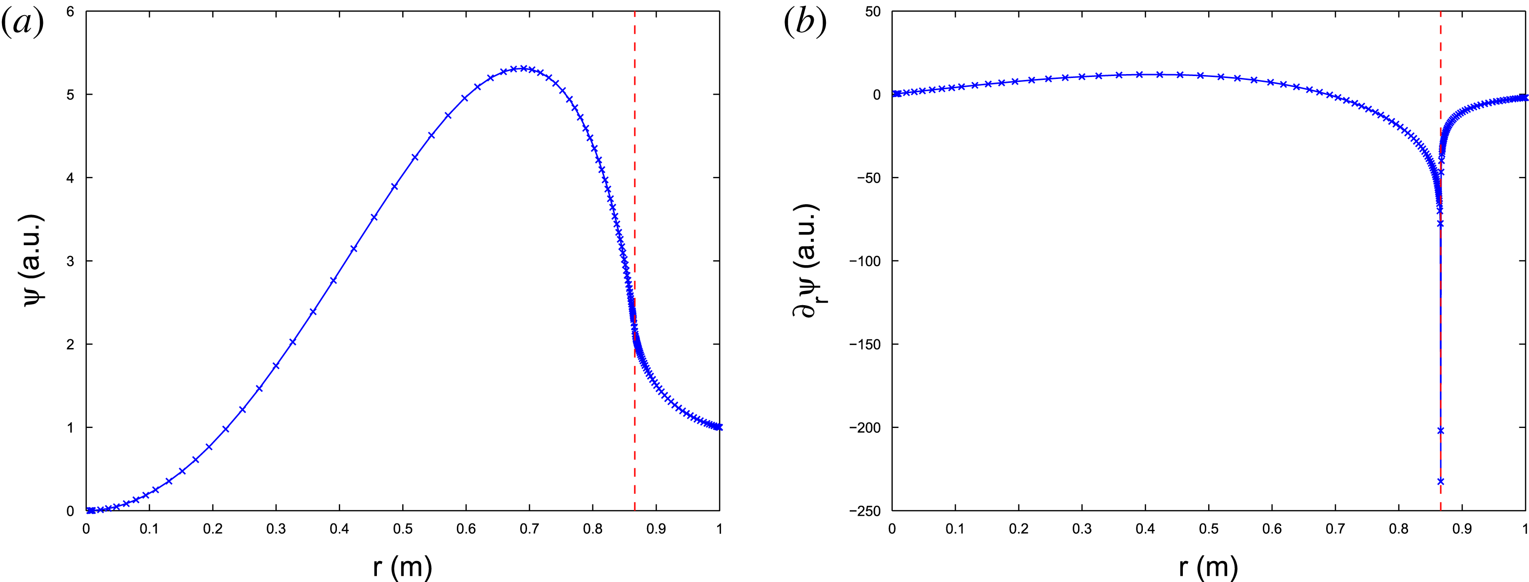
An example of the
 $2/1$
mode structure for a parabolic current profile with
 ${\it\beta}=0$
: (a) the perturbed helical flux
 ${\it\psi}$
, and (b) its radial gradient
 $\partial _{r}{\it\psi}$
. Both are in arbitrary units.

The coefficients
 $a_{2}$
,
 $b_{1},b_{2}$
are determined by expansion of
 $G$
near the resonance. Recall that
 $B_{z}/R=1$
, so that
 $F=({\it\mu}-{\it\mu}_{s})$
. Then,
 $$\begin{eqnarray}\displaystyle G & \equiv & \displaystyle \frac{m^{2}}{r}+\frac{j^{\prime }}{F}\nonumber\\ \displaystyle & = & \displaystyle \frac{m^{2}}{r_{s}}-\frac{m^{2}}{r_{s}r}x+\frac{1}{{\it\mu}^{\prime }x}\frac{j^{\prime }+j^{\prime \prime }x}{1+{\it\mu}_{2}x}\nonumber\\ \displaystyle & = & \displaystyle \frac{\hat{T}}{x}+\frac{m^{2}}{r_{s}}-\left(\hat{T}{\it\mu}_{2}-\frac{j^{\prime \prime }}{{\it\mu}^{\prime }}\right)\frac{1}{1+{\it\mu}_{2}x}-\frac{m^{2}}{r_{s}r}x\nonumber\\ \displaystyle & = & \displaystyle \frac{\hat{T}}{x}+g_{0}+\tilde{G},\end{eqnarray}$$
where
 $$\begin{eqnarray}\hat{T}\equiv \frac{j^{\prime }}{{\it\mu}^{\prime }},\quad {\it\mu}_{2}\equiv \frac{{\it\mu}_{s}^{\prime \prime }}{2{\it\mu}_{s}},\quad g_{0}=-\left(\hat{T}{\it\mu}_{2}-\frac{j^{\prime \prime }}{{\it\mu}^{\prime }}\right),\quad \tilde{G}_{x=0}=0.\end{eqnarray}$$
This gives
 $$\begin{eqnarray}\displaystyle & \displaystyle 2r_{s}a_{2}+1=\hat{T},\quad b_{1}=\frac{\hat{T}}{r_{s}},\quad 2b_{2}=\frac{g_{0}-2b_{1}}{r_{s}}-3b_{1}a_{2}, & \displaystyle\end{eqnarray}$$
 $$\begin{eqnarray}\displaystyle & \displaystyle {\it\Gamma}_{1}=(\hat{T}a_{2}+g_{0}-4a_{2})x+(g_{0}a_{2}+\tilde{G})x^{2}+a_{2}\tilde{G}x^{3}, & \displaystyle\end{eqnarray}$$
 $$\begin{eqnarray}\displaystyle {\it\Gamma}_{2} & = & \displaystyle b_{1}(a_{2}\hat{T}+g_{0}-4a_{2})x\ln |x|+(\hat{T}b_{2}+\tilde{G}-4a_{2}b_{1}-4b_{2})\frac{1}{r_{s}}x\nonumber\\ \displaystyle & & \displaystyle +\,\{\tilde{G}b_{1}\ln |x|+(g_{0}+\tilde{G}x)[b_{1}a_{2}\ln |x|+b_{2}]\}x^{2},\end{eqnarray}$$
near the resonant surface. Now the equations for
 $U_{1},U_{2}$
have no singularities and the stability parameter
 ${\it\Delta}^{\prime }$
is determined simply by
 $$\begin{eqnarray}{\it\Delta}^{\prime }\equiv \left.\frac{{\it\psi}_{s}^{\prime }}{{\it\psi}_{s}}\right|_{-}^{+}=\frac{U_{1}^{(+)}-U_{1}^{(-)}}{U_{2s}}.\end{eqnarray}$$
Figure 1 shows an example of mode structure for a parabolic current profile:
 $$\begin{eqnarray}j(r)=j(0)\left(1-\frac{r^{2}}{a^{2}}\right).\end{eqnarray}$$
Here, the minor radius
 $a=1$
, the major radius
 $R=10$
and the toroidal field
 $B_{t}=10$
with the central safety factor
 $q_{0}=1.25$
and edge safety factor
 $q_{a}=2.5$
. The position of the resonant surface for the
 $2/1$
mode is
 $r_{s}=0.8662$
. The mode structure is calculated by solving the original ideal equation (3.1) while switching to the expansion method of this section near the resonant point. The numerical integration is carried out by LSODE (Hindmarsh Reference Hindmarsh1980).
4. Special kind of profile for high
${\it\beta}$
ideal solution study

The pressure gradient in (2.34) introduces a singularity
 $\propto 1/x^{2}$
and changes the form of the two asymptotic solutions
 $u_{1}$
and
 $u_{2}$
. In order to be closer to a real toroidal plasma, we consider an equation of the following form:
 $$\begin{eqnarray}(r{\it\psi}^{\prime })^{\prime }=G{\it\psi},\quad G\equiv \frac{m^{2}}{r}+\frac{j^{\prime }}{F}-2k^{2}\frac{p_{o}^{\prime }}{F^{2}}\left(1-\frac{m^{2}}{n^{2}}\right),\end{eqnarray}$$
where the factor
 $(1-m^{2}/n^{2})$
mimics the toroidal effect of averaged curvature (Zakharov Reference Zakharov1978). The two asymptotic solutions have the following forms:
 $$\begin{eqnarray}\displaystyle & \displaystyle u_{1}=|x|^{{\it\nu}}[x+a_{2}x^{2}+\cdots \,], & \displaystyle\end{eqnarray}$$
 $$\begin{eqnarray}\displaystyle & \displaystyle u_{2}=|x|^{-{\it\nu}}[1+b_{1}x+b_{2}x^{2}+\cdots \,]. & \displaystyle\end{eqnarray}$$
In the above equations,
 ${\it\nu}$
is the Suydam–Mercier index (Suydam Reference Suydam1958; Mercier Reference Mercier1962) for the tokamak geometry, which is generally positive and will increase as the pressure gradient steepens. As mentioned in the Introduction, attempts to solve this equation using the same asymptotic technique described in § 3 would meet obvious difficulties because of this form of expansion. First, as
 ${\it\nu}$
increases, the large solution will be increasingly dominant over the small solution, and this requires keeping more and more terms in
 $u_{2}$
and higher-order radial derivatives in
 $G$
. (Regarding
 $u_{1}$
, two expansion terms are sufficient.) Moreover, even if this were successful, the residual term
 $\tilde{G}$
, which can be of high order in
 $x$
, could be obscured by finite numerical accuracy due to a small difference of large terms. The second and fundamental problem is the need for high-order derivatives of the equilibrium plasma profiles and the geometry of the magnetic configurations, which are not available in practice. The equilibrium equations do not contain high-order derivatives.
Here we introduce specially designed current and pressure profiles to eliminate the aforementioned difficulties. Specifically, we choose
 $G$
in the following form near the resonance:
 $$\begin{eqnarray}G=G_{0}+\frac{G_{-1}}{x}+\frac{G_{-2}}{x^{2}},\quad G_{0}\equiv \frac{m^{2}}{r_{s}},\quad G_{-1}=\text{const.},G_{-2}=\text{const}.\end{eqnarray}$$
The current profile is determined by the equation
 $$\begin{eqnarray}j^{\prime }=\frac{F}{x}G_{-1}+\frac{m^{2}}{r_{s}r}Fx.\end{eqnarray}$$
while the pressure profile by
 $$\begin{eqnarray}-2k^{2}p_{0}^{\prime }\left(1-\frac{m^{2}}{n^{2}}\right)=\frac{F^{2}}{x^{2}}G_{-2}.\end{eqnarray}$$
Both the values and first derivatives of the pressure and current density match their profiles outside the resonant region.
We first construct the current profile
 $j$
and introduce an additional unknown variable
 $X$
as
 $$\begin{eqnarray}X\equiv \frac{1}{x}\int _{r_{s}}^{r}rj\,\text{d}r.\end{eqnarray}$$
For our purpose, they should obey two first-order ordinary differential equations
 $$\begin{eqnarray}\displaystyle & \displaystyle r^{3}j^{\prime }=\left(G_{-1}r+\frac{m^{2}}{r_{s}}x^{2}\right)[X-(2r_{s}+x){\it\mu}_{s}], & \displaystyle\end{eqnarray}$$
 $$\begin{eqnarray}\displaystyle & \displaystyle (xX)^{\prime }=rj. & \displaystyle\end{eqnarray}$$
The two free parameters of these equations can be used to match the current density and its derivative at the left side of the resonant region. Then, the current profile in the right outer region can be designed specially to make a smooth transition from the resonant zone.
In fact, the current density profile in the resonant zone can be generated using the expansion
 $$\begin{eqnarray}X\equiv \frac{1}{x}\int _{0}^{x}(r_{s}+x)j\,\text{d}x=X_{0}+\mathop{\sum }_{k=1}\frac{1}{k!}X_{k}x^{k}.\end{eqnarray}$$
Substituting (4.9) into (4.8), we get:
 $$\begin{eqnarray}r^{2}(xX)^{\prime \prime }-r(xX)^{\prime }=\left(G_{-1}r+\frac{m^{2}}{r_{s}}x^{2}\right)[X-(2r_{s}+x){\it\mu}_{s}],\end{eqnarray}$$
which leads to the expansion
 $$\begin{eqnarray}\displaystyle & \displaystyle 2r_{s}X_{1}=(G_{-1}+1)X_{0}-2{\it\mu}_{s}r_{s}G_{-1}, & \displaystyle\end{eqnarray}$$
 $$\begin{eqnarray}\displaystyle & \displaystyle 3r_{s}X_{2}=G_{-1}X_{1}-{\it\mu}_{s}G_{-1}, & \displaystyle\end{eqnarray}$$
 $$\begin{eqnarray}\displaystyle & \displaystyle 4r_{s}X_{3}=(G_{-1}-3)X_{2}+2\frac{m^{2}}{r_{s}^{2}}(X_{0}-2r_{s}{\it\mu}_{s}), & \displaystyle\end{eqnarray}$$
 $$\begin{eqnarray}\displaystyle & \displaystyle 5r_{s}X_{4}=(G_{-1}-8)X_{3}-6\frac{m^{2}}{r_{s}^{3}}(X_{0}-r_{s}X_{1}-r_{s}{\it\mu}_{s}), & \displaystyle\end{eqnarray}$$
 $$\begin{eqnarray}\displaystyle (k+2)r_{s}X_{k+1} & = & \displaystyle [G_{-1}+1-k^{2}]X_{k}+\frac{m^{2}}{r_{s}^{2}}k(k-1)X_{k-2}\nonumber\\ \displaystyle & & \displaystyle +\,k[-(k-1)^{2}+G_{-1}+1]\frac{1}{r_{s}}X_{k-1}-[(k+1)k]X_{k}\quad \text{for }k\geqslant 4.\qquad\end{eqnarray}$$
The parameters
 $G_{-1}$
and
 $X_{0}$
can be considered to be free parameters.
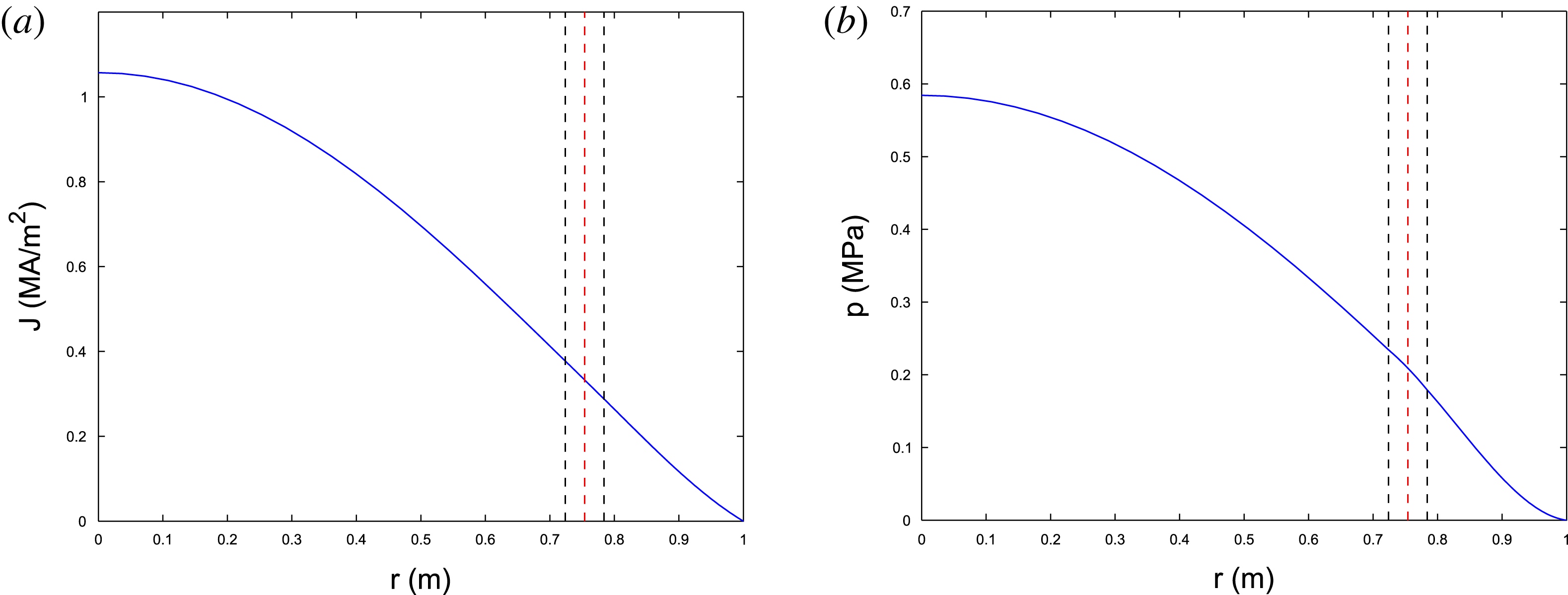
The special pressure profile can be generated using the first order ODE (4.6). Figure 2 shows an example of current and pressure profiles for the
 $3/1$
mode given the special form of
 $G$
with
 $G_{-1}=3.358$
,
 $G_{-2}=8.294\times 10^{-2}$
and
 $r_{s}=0.754$
.
The (a) current and (b) pressure profiles specially generated to satisfy (4.5) and (4.6) near the resonance. The red dashed line denotes the resonant surface for
 $3/1$
mode. The two black dashed lines denote the resonant region where the special profiles are used. The profiles and their first derivative are matched profiles in the outer regions.

5. Behaviour of the ideal solution near the resonant point for
${\it\beta}\neq 0$
plasmas

The Robinson method, described in § 3 by (3.1)–(3.6), is applicable also in the case of a second-order singularity and the special profiles of the previous section provide a classical form of eigen-equation, which can be solved to arbitrary numerical accuracy.
The
 ${\it\nu}$
parameter defined through the Suydam–Mercier index for ideal interchange stability (Suydam Reference Suydam1958; Mercier Reference Mercier1962)
 $$\begin{eqnarray}{\it\nu}=-\frac{1}{2}+\sqrt{\frac{1}{4}+\frac{2k^{2}R^{2}p^{\prime }}{{\it\mu}_{s}^{\prime 2}r_{s}B_{z}^{2}}\left(1-\frac{m^{2}}{n^{2}}\right)}\end{eqnarray}$$
causes some modification of the asymptotic solutions when
 $2{\it\nu}$
is close to integer by introducing logarithm terms.
It is worthwhile to note that in tokamaks,
 $1-m^{2}/n^{2}$
is usually negative and the pressure contribution is positive, thus making
 ${\it\nu}$
positive.
In the following subsections, we will investigate the
 $2{\it\nu}$
non-integer and
 $2{\it\nu}$
integer cases separately. In particular, we describe how to remove the singularity in the coefficients in the second case.
5.1. Extraction of solution near resonance for
$2{\it\nu}$
not integer

Here, we demonstrate how to obtain the asymptotic solutions and functions
 ${\it\Gamma}_{1},{\it\Gamma}_{2}$
in (3.1)–(3.6) for
 $U_{1},U_{2}$
to the sixth order in
 $x$
assuming that
 ${\it\nu}<2$
.
The cancellation in lowest-order terms for both
 ${\it\Gamma}_{1}$
and
 ${\it\Gamma}_{2}$
yield:
 $$\begin{eqnarray}{\it\nu}=-\frac{1}{2}+\sqrt{\frac{1}{4}+\frac{G_{-2}}{r_{s}}},\end{eqnarray}$$
which is the expression of the Suydam–Mercier index (Suydam Reference Suydam1958; Mercier Reference Mercier1962). The cancellation of
 $O(x^{0})$
order terms in
 ${\it\Gamma}_{1}$
gives the value of
 $a_{2}$
:
 $$\begin{eqnarray}G_{-1}-(1+{\it\nu})^{2}-2(1+{\it\nu})a_{2}r_{s}=0.\end{eqnarray}$$
For higher orders,
 $O(x^{n})$
with
 $n\geqslant 1$
(
 $a_{1}\equiv 1$
):
 $$\begin{eqnarray}-(n+1)(n+2+2{\it\nu})a_{n+2}r_{s}+[G_{-1}-(n+1+{\it\nu})^{2}]a_{n+1}+G_{0}a_{n}=0.\end{eqnarray}$$
Similarly, the cancellation in the
 $O(x^{-1})$
order in
 ${\it\Gamma}_{2}$
gives
 $b_{1}$
:
 $$\begin{eqnarray}G_{-1}-{\it\nu}^{2}+2{\it\nu}b_{1}r_{s}=0.\end{eqnarray}$$
For any higher order,
 $O(x^{n})$
with
 $n\geqslant 0$
, we have:
 $$\begin{eqnarray}-(n+2)(n+1-2{\it\nu})b_{n+2}r_{s}+[G_{-1}-(n+1-{\it\nu})^{2}]b_{n+1}+G_{0}b_{n}=0.\end{eqnarray}$$
We can find all of the coefficients in
 $u_{1}$
and
 $u_{0}$
by using the above equations iteratively. Further, we now can write down the expressions for
 ${\it\Gamma}_{1}|x|^{-{\it\nu}}$
and
 ${\it\Gamma}_{2}|x|^{{\it\nu}}$
, where only
 $o(x^{5})$
and higher-order terms are non-zero:
 $$\begin{eqnarray}\displaystyle & \displaystyle {\it\Gamma}_{1}|x|^{-{\it\nu}}=[-(6+{\it\nu})^{2}a_{6}+(G_{-1}a_{6}+G_{0}a_{5})+G_{0}a_{6}x]x^{5}, & \displaystyle\end{eqnarray}$$
 $$\begin{eqnarray}\displaystyle & \displaystyle {\it\Gamma}_{2}|x|^{{\it\nu}}=[-(6-{\it\nu})^{2}b_{6}+(G_{-1}b_{6}+G_{0}b_{5})+G_{0}b_{6}x]x^{5}. & \displaystyle\end{eqnarray}$$
 ${\it\Gamma}_{1}$
and
 ${\it\Gamma}_{2}$
can then be used to advance
 $U_{1}$
and
 $U_{2}$
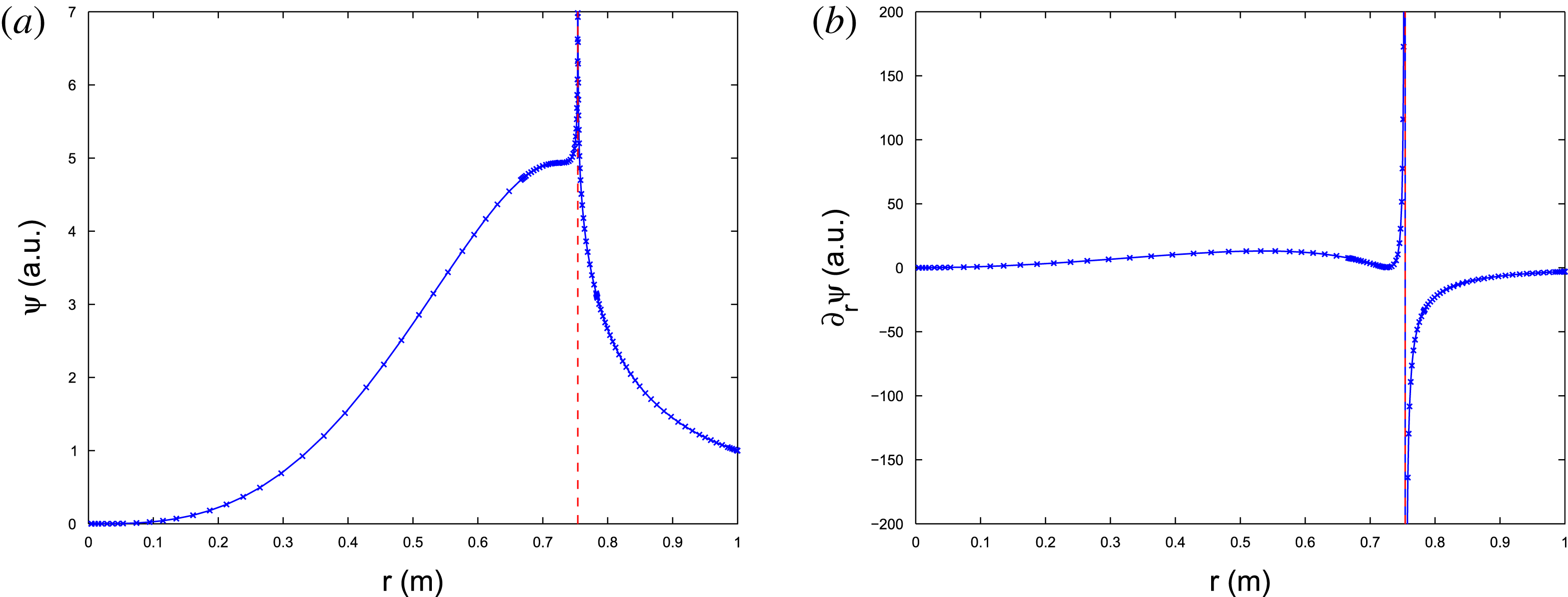
by (3.5). An example of the
 $3/1$
mode structure is shown in figure 3 calculated using the current and pressure profile shown in figure 2, with central safety factor
 $q(0)=1.892$
and edge safety factor
 $q(a)=4.521$
. The singularity in both the value and the first derivative of the mode structure is evident, as opposed to the low
 ${\it\beta}$
case shown in figure 1 where only the first derivative of the mode structure is singular.
An example of a
 $3/1$
mode structure calculated using special profiles of § 4. The singularity in both the value of perturbed helical flux and its derivative is evident. (a) The perturbed helical flux
 ${\it\psi}$
, and (b) its radial derivative
 $\partial _{r}{\it\psi}$
.

5.2. Extraction of the solution near resonance for
$2{\it\nu}$
integer

As can be seen in (5.6), when
 $n+1-2{\it\nu}$
approaches zero, the coefficient
 $b_{n+2}$
becomes singular, indicating the necessity to change the form of the
 $u_{2}$
solution. Let us consider a small quantity,
 ${\it\alpha}=k+1-2{\it\nu}$
, while
 $k$
is a given integer. The smallness of
 ${\it\alpha}$
means that we have the following expansion:
 $$\begin{eqnarray}|x|^{{\it\alpha}}\sim 1+{\it\alpha}\text{ln}|x|.\end{eqnarray}$$
Bearing this expansion in mind, we construct a new asymptotic solution
 $u_{2}$
to (4.1)
 $$\begin{eqnarray}u_{2}=|x|^{-{\it\nu}}[1+b_{1}x+b_{2}x^{2}+\cdots +b_{6}x^{6}]+u_{0L},\end{eqnarray}$$
where
 $$\begin{eqnarray}u_{0L}\equiv Lu_{1}(x^{{\it\alpha}}-1).\end{eqnarray}$$
Here,
 $L$
is a constant coefficient. The form of
 $u_{1}$
is not affected.
The cancellation of all terms lower than
 $O(x^{k})$
yields the same result as in the previous case:
 $$\begin{eqnarray}-(n+2)(n+1-2{\it\nu})b_{n+2}r_{s}+[G_{-1}-(n+1-{\it\nu})^{2}]b_{n+1}+G_{0}b_{n}=0\quad \text{for }n<k.\end{eqnarray}$$
While at the
 $x^{k}$
order, we have
 $$\begin{eqnarray}-({\it\alpha}+2{\it\nu}+1){\it\alpha}b_{k+2}r_{s}+[G_{-1}-(n+1-{\it\nu})^{2}]b_{k+1}+G_{0}b_{k}-({\it\alpha}+2{\it\nu}+1){\it\alpha}Lr_{s}=0.\end{eqnarray}$$
For extremely small
 ${\it\alpha}$
,
 ${\it\alpha}L$
is just the coefficient in front of the logarithm term. In the case of
 ${\it\alpha}\sim 0$
, we choose
 $L$
in such a way that the sum of last three terms on the left-hand side approach zero faster than
 ${\it\alpha}$
. In this way the singularity in
 $b_{k+2}$
can be resolved. A simple choice is to make the last three terms exactly cancel each other, so that
 $b_{k+2}=0$
even for
 ${\it\alpha}\sim 0$
. So that, formally, we have:
 $$\begin{eqnarray}\displaystyle & \displaystyle b_{k+2}=0, & \displaystyle\end{eqnarray}$$
 $$\begin{eqnarray}\displaystyle & \displaystyle ({\it\alpha}+2{\it\nu}+1){\it\alpha}Lr_{s}=[G_{-1}-(n+1-{\it\nu})^{2}]b_{k+1}+G_{0}b_{k}. & \displaystyle\end{eqnarray}$$
For convenience, we now define the following new coefficient:
 $$\begin{eqnarray}{\it\Lambda}_{n}\equiv (2n-k+1)a_{n-k}+(2n-k+2)a_{n-k+1}r_{s}.\end{eqnarray}$$
It follows that, for any term with order higher than
 $O(x^{k})$
, the iterative relationship becomes:
 $$\begin{eqnarray}-(n+2)(n+1-2{\it\nu})b_{n+2}+[G_{-1}-(n+1-{\it\nu})^{2}]b_{n+1}+G_{0}b_{n}-{\it\Lambda}_{n}{\it\alpha}L=0\quad \text{for }n>k.\end{eqnarray}$$
With all the coefficients in
 $u_{1}$
and
 $u_{2}$
known, we can proceed to write
 ${\it\Gamma}_{1}$
and
 ${\it\Gamma}_{2}$
:
 $$\begin{eqnarray}\displaystyle & \displaystyle {\it\Gamma}_{1}=[-(6+{\it\nu})^{2}a_{6}+(G_{-1}a_{6}+G_{0}a_{5})+G_{0}a_{6}x]x^{5}|x|^{{\it\nu}}, & \displaystyle\end{eqnarray}$$
 $$\begin{eqnarray}\displaystyle & \displaystyle {\it\Gamma}_{2}=\left[-(6-{\it\nu})^{2}b_{6}+(G_{-1}b_{6}+G_{0}b_{5})+G_{0}b_{6}x-\mathop{\sum }_{n=5}^{6+k}{\it\Lambda}_{n}x^{n-5}{\it\alpha}L\right]x^{5}|x|^{-{\it\nu}}+L{\it\Gamma}_{1}(x^{{\it\alpha}}-1).\hspace{-6.0pt} & \displaystyle \nonumber\\ \displaystyle & & \displaystyle\end{eqnarray}$$
Note that the low
 ${\it\beta}$
asymptotic solutions can be recovered by simply considering
 ${\it\nu}$
to approach zero.
5.3. Dominant mode structure behaviour near resonance for high
${\it\beta}$
plasma

At the resonant point, the asymptotic method requires
 $$\begin{eqnarray}U_{2}^{(+)}=U_{2}^{(-)}\equiv U_{2s}.\end{eqnarray}$$
Because for
 ${\it\beta}\neq 0$
the large solution
 $u_{2}$
is singular, the condition
 ${\it\nu}>0$
indicates linear resistive stability, while for
 ${\it\nu}<0$
an instability occurs when
 ${\it\eta}\rightarrow 0$
. For finite conductivity and the existence of a resistive resonant layer, the contributions from both solutions should be taken into account.
The derivative of the full solution near resonance is given by
 $$\begin{eqnarray}{\it\psi}^{\prime }\sim -{\it\nu}|x|^{-{\it\nu}}x^{-1}U_{2}+(1+{\it\nu})|x|^{{\it\nu}}U_{1}.\end{eqnarray}$$
Assuming the half-width of the resistive layer to be
 $x_{{\it\eta}}$
, the linear drive
 ${\it\Delta}^{\prime }$
is:
 $$\begin{eqnarray}{\it\Delta}^{\prime }\equiv \frac{{\it\psi}^{\prime }|_{-}^{+}}{{\it\psi}_{s}}=-2{\it\nu}x_{{\it\eta}}^{-1}+{\it\Delta}_{\ast }^{\prime }({\it\nu}+1)|x_{{\it\eta}}|^{2{\it\nu}},\end{eqnarray}$$
where
 $$\begin{eqnarray}{\it\Delta}_{\ast }^{\prime }\equiv \frac{(U_{1+}-U_{1-})}{U_{2s}}.\end{eqnarray}$$
It can be seen that the first term on the right-hand side of (5.22) is strongly stabilizing for small
 $x_{{\it\eta}}$
. This is the origin of pressure gradient stabilization in the Glasser effect.
In the presence of a finite island, the tearing layer width
 $x_{{\it\eta}}$
should be replaced by island semi-width
 $w$
. Its critical value
 $w_{c}$
, beyond which the Glasser effect is no longer effective, is determined by the balance of two terms on the right-hand side of (5.22):
 $$\begin{eqnarray}w_{c}^{2{\it\nu}+1}{\it\Delta}_{\ast }^{\prime }=\frac{2{\it\nu}}{1+{\it\nu}}.\end{eqnarray}$$
This result essentially agrees with Kotschenreuther et al. (Reference Kotschenreuther, Hazeltine and Morrison1985). We note that
 $2{\it\nu}+1$
here is the power ‘
 $p$
’ in Kotschenreuther et al. (Reference Kotschenreuther, Hazeltine and Morrison1985) and using those notations
 $$\begin{eqnarray}{\it\nu}=-{\textstyle \frac{1}{2}}+\sqrt{{\textstyle \frac{1}{4}}-D_{I}}.\end{eqnarray}$$
Then the right-hand side of (5.24) is
 $$\begin{eqnarray}\frac{2{\it\nu}}{1+{\it\nu}}=-2\frac{(1-\sqrt{1-4D_{I}})^{2}}{4D_{I}}.\end{eqnarray}$$
For the small
 $D_{I}$
assumed in Kotschenreuther et al. (Reference Kotschenreuther, Hazeltine and Morrison1985)
 $$\begin{eqnarray}\sqrt{1-4D_{I}}\simeq 1-2D_{I},\quad \frac{2{\it\nu}}{1+{\it\nu}}=-2D_{I}.\end{eqnarray}$$
Recall that
 $D_{I}\equiv E+F+H$
and
 $E\sim F\sim H$
in the notation of Kotschenreuther et al. (Reference Kotschenreuther, Hazeltine and Morrison1985), and the cases we are interested in have
 $E+F\sim E+F+H<0$
. Hence we can finally write down the following critical island width for small
 $|E+F|$
:
 $$\begin{eqnarray}w_{c}^{2{\it\nu}+1}{\it\Delta}_{\ast }^{\prime }\sim K|E+F|,\end{eqnarray}$$
where
 $K$
is a constant determined by the geometry. This reproduces the main result of Kotschenreuther et al. (Reference Kotschenreuther, Hazeltine and Morrison1985), indicating that only the outer region determines the stability condition of the resistive modes.
6. Profile modification for a finite island size
The linear mode structures for both low
 ${\it\beta}$
and high
 ${\it\beta}$
cases were dealt with in previous sections. As discussed previously, solving the ideal linear mode structure is equivalent to seeking the nearest equilibrium from an unperturbed one. The perturbed equilibrium will have a singular feature at the resonant surface. In a real plasma, however, the ideal linear mode does not exist. The inclusion of any finite dissipation near the resonant surface will resolve the singularity and result in the formation of magnetic islands on those surfaces (White Reference White1986). While very thin islands would be ‘short circuited’ by transport processes perpendicular to the flux surfaces, for larger islands, the temperature, density, pressure and consequently current density profile will be effectively flattened (Fitzpatrick Reference Fitzpatrick1995; Yu Reference Yu2006). This is due to the fact that the parallel transport is much stronger than the cross-field line perpendicular transport. Our interest is in consideration of larger islands and marginal points where the island is wide enough to saturate, or alternatively, wide enough to overcome the Glasser effect. Hence, hereafter, we consider islands with pressure and current density profiles flattened. The non-flat profiles within the island can be added as the second derivative term as long as the profile is still a function of helical flux. Such profiles may be of interest for investigating the thermal instability caused by island cooling (Gates & Delgato-Aparicio Reference Gates and Delgato-Aparicio2012; White et al.
Reference White, Gates and Brennan2015).
The purpose of this section is to analyse the profile modification caused by a finite size island, which is essentially a 2-D effect. However, we found that the 2-D effect is important only within a radial region of the island size, while outside it, the linear approximation based on a modified zeroth harmonic is sufficient. Hence, outside the island radial zone, we will express the principal harmonic of the perturbed current density using the ideal linear mode formalism. In the island region both zeroth and principal harmonics are calculated using a 2-D geometry assuming its equilibrium, current density and pressure profiles are functions of the helical flux
 ${\it\Psi}^{\ast }$
(Rutherford Reference Rutherford1973).
The flux function near the resonant point can be represented by the following equation (Zakharov Reference Zakharov1986):
 $$\begin{eqnarray}{\it\Psi}^{\ast }(x,{\it\theta})={\it\Psi}_{0s}^{\ast }+{\textstyle \frac{1}{2}}{\it\Psi}_{0s}^{\prime \prime }x^{2}+({\it\psi}_{s}+{\it\psi}_{s}^{\prime }x)\cos m{\it\theta}.\end{eqnarray}$$
where
 $x$
is the radial distance to the resonant surface, and the subscript ‘
 $s$
’ denotes the value taken at the resonant surface. For now, the values of
 ${\it\psi}_{s}$
and
 ${\it\psi}_{s}^{\prime }$
are considered as given parameters. Later, they will be self-consistently calculated when we are attempting to find the marginal stable point. In iteration toward an equilibrium, the values of
 ${\it\psi}^{\prime }$
on opposite sides of the resonant surface may be different.
The island semi-width
 $w$
and the asymmetry
 $s$
of the island are determined by
 $$\begin{eqnarray}w=2\sqrt{-{\it\psi}_{s}/{\it\Psi}_{0s}^{\prime \prime }},\quad s={\it\psi}_{s}^{\prime }/{\it\Psi}_{0s}^{\prime \prime }.\end{eqnarray}$$
The 2-D magnetic surfaces of the island region are described by
 $$\begin{eqnarray}\frac{2({\it\Psi}^{\ast }-{\it\Psi}_{0s}^{\ast })}{{\it\Psi}_{0s}^{\prime \prime }}=x^{2}-w^{2}\cos ^{2}\frac{m{\it\theta}}{2}+2xs\cos m{\it\theta}+\frac{w^{2}}{2}.\end{eqnarray}$$
The geometry of the separatrix is determined by the equation
 ${\it\Psi}^{\ast }={\it\Psi}_{S}^{\ast }$
, where
 ${\it\Psi}_{S}^{\ast }$
is the helical flux at the X-point (the saddle point in the profile of the helical flux)
 $$\begin{eqnarray}{\it\Psi}_{S}^{\ast }={\it\Psi}_{0s}^{\ast }+\frac{1}{2}{\it\Psi}_{0s}^{\prime \prime }\left(\frac{w^{2}}{2}-s^{2}\right).\end{eqnarray}$$
Let
 $x_{Sl}$
and
 $x_{Sr}$
denote the left and right boundaries of the separatrix:
 $$\begin{eqnarray}\displaystyle & \displaystyle x_{Sl}({\it\theta})=-x_{S0}-s\cos m{\it\theta}, & \displaystyle\end{eqnarray}$$
 $$\begin{eqnarray}\displaystyle & \displaystyle x_{Sr}({\it\theta})=x_{S0}-s\cos m{\it\theta}, & \displaystyle\end{eqnarray}$$
 $$\begin{eqnarray}\displaystyle & \displaystyle x_{S0}\equiv \left|w\cos \frac{m{\it\theta}}{2}\right|. & \displaystyle\end{eqnarray}$$
Equations (6.5)–(6.7) clearly state that
 $w$
corresponds to the semi-width of the island, while
 $s$
induces a periodic asymmetry for the island along the poloidal direction. Asymmetry results in the outward shift of the X-point and inward shift of O-point (the point of the minimum in the profile of the helical flux) of the island. As
 $s$
is essentially
 ${\it\psi}_{s}^{\prime }$
, the island asymmetry is the indication that
 ${\it\psi}$
is not constant across the island. A contour of the helical flux
 ${\it\Psi}$
is shown in figure 4, where the geometry of the island and the asymmetry is evident.
A sample contour of the total helical flux
 ${\it\Psi}^{\ast }$
near the resonant surface
 $x=0$
projected into the slab geometry. The red dashed line represent the position of the resonant surface, while the black point denotes the position of island O-point. The radial region between the two blue dashed lines is the 2-D region where 2-D profile modification is dominant. Outside the region, the zeroth harmonic of the modified profile serves as a good approximation.

Now, we can describe the geometry near the resonant surface by introducing the following flux-coordinate with the dimension of
 $x^{2}$
:
 $$\begin{eqnarray}{\it\chi}({\it\Psi})\equiv \frac{2({\it\Psi}-{\it\Psi}_{S})}{{\it\Psi}_{0}^{\prime \prime }}=x^{2}-x_{S0}^{2}+s^{2}+2xs\cos m{\it\theta}.\end{eqnarray}$$
When the island geometry is known, the current density profile can be represented by the leading term in the expansion in the island size (Zakharov Reference Zakharov1986):
 $$\begin{eqnarray}j({\it\chi})=\left\{\begin{array}{@{}lll@{}}j_{0} & -j_{l}^{\prime }(\sqrt{{\it\chi}+d_{l}^{2}}-d_{l}) & +{\textstyle \frac{1}{2}}j_{l}^{\prime \prime }{\it\chi},\quad (x<x_{Sl})\\ j_{0} & & +{\textstyle \frac{1}{2}}j_{i}^{\prime \prime }{\it\chi},\quad (x_{Sl}<x<x_{Sr}),\\ j_{0} & +j_{r}^{\prime }(\sqrt{{\it\chi}+d_{r}^{2}}-d_{r}) & +{\textstyle \frac{1}{2}}j_{r}^{\prime \prime }{\it\chi},\quad (x<x_{Sr}),\end{array}\right.\end{eqnarray}$$
where
 $d_{l}\equiv w_{l}+s$
,
 $d_{r}\equiv w_{r}-s$
, and
 $w_{l}\equiv w+s$
,
 $w_{r}\equiv w-s$
. Here,
 $d_{l}$
and
 $d_{r}$
represent the radial distance between the extreme points of the island and the X-point,
 $w_{l}$
and
 $w_{r}$
represent the radial position of those extreme points:
 $w_{l}=-x_{sl}(0)$
,
 $w_{r}=x_{sr}(0)$
. The values
 $j_{0}$
,
 $j_{lr}^{\prime }$
and
 $j_{lr}^{\prime \prime }$
should be seen as constant parameters determined by the matching of the modified and unperturbed profiles at some distance from the island zone. As mentioned, the non-flat island profile will enter as the
 $j_{i}^{\prime \prime }$
term, representing possible cooling, heating or other mechanism which may alter profiles within the island. Unless large, this term does not affect the quasilinear equilibrium and for the purpose of this paper, we let
 $j_{i}^{\prime \prime }$
be zero.
It can be seen from (6.9) that the current modification is 2-D in nature. However, numerical observation indicates that the ideal linear approximation for the perturbed current density based on the zeroth harmonic of 2-D modification serves as a pretty good approximation outside the island width, providing less than one percent deviation from the 2-D result. Hence it is possible to use the simple linearized profile modification outside the island zone first, while dealing with the 2-D profile modification within the island.
First, let us consider the behaviour of the current profile outside the island. Its zeroth harmonic
 $$\begin{eqnarray}j^{(0)}(x)\equiv \frac{1}{2{\rm\pi}}\int _{-{\rm\pi}}^{{\rm\pi}}j({\it\chi})\,\text{d}{\it\theta}\end{eqnarray}$$
for
 $x<x_{sl}$
and
 $x>x_{sr}$
is given by
 $$\begin{eqnarray}\displaystyle & \displaystyle j^{(0)}(x)=j_{0}-j_{l}^{\prime }X_{1l}+{\textstyle \frac{1}{2}}\,j_{l}^{\prime \prime }X_{2}^{2},\quad (x<x_{Sl}) & \displaystyle\end{eqnarray}$$
 $$\begin{eqnarray}\displaystyle & \displaystyle j^{(0)}(x)=j_{0}+j_{r}^{\prime }X_{1r}+{\textstyle \frac{1}{2}}\,j_{r}^{\prime \prime }X_{2}^{2},\quad (x>x_{Sr}), & \displaystyle\end{eqnarray}$$
where
 $$\begin{eqnarray}\displaystyle & \displaystyle X_{1l}=-d_{l}+\frac{2}{{\rm\pi}}\sqrt{d_{l}^{2}+(x-s)^{2}}E\left(\frac{w^{2}-4sx}{d_{l}^{2}+(x-s)^{2}}\right), & \displaystyle\end{eqnarray}$$
 $$\begin{eqnarray}\displaystyle & \displaystyle X_{1r}=-d_{r}+\frac{2}{{\rm\pi}}\sqrt{d_{r}^{2}+(x-s)^{2}}E\left(\frac{w^{2}-4sx}{d_{r}^{2}+(x-s)^{2}}\right), & \displaystyle\end{eqnarray}$$
 $$\begin{eqnarray}\displaystyle & \displaystyle X_{2}^{2}={\textstyle \frac{1}{2}}(2x^{2}+2s^{2}-w^{2}). & \displaystyle\end{eqnarray}$$
Here,
 $E(x)$
is the complete elliptic integral of the second kind:
 $$\begin{eqnarray}E(x)=\int _{0}^{{\rm\pi}/2}(1-x\sin ^{2}{\it\theta})^{1/2}\,\text{d}{\it\theta}.\end{eqnarray}$$
The parameters
 $j_{0}$
,
 $j_{l}^{\prime }$
,
 $j_{l}^{\prime \prime }$
,
 $j_{r}^{\prime }$
,
 $j_{r}^{\prime \prime }$
are determined by the condition that (6.10) must match onto the value and derivative of the unperturbed
 $j$
-profile at a distance from the island.
Inside the island 2-D zone, the presence of a separatrix must be considered. This 2-D region is essentially defined by the radial region between the two extreme points of the island, as is shown in figure 4 between the blue dashed lines. The
 $\sqrt{{\it\chi}+d_{l}^{2}}$
and
 $\sqrt{{\it\chi}+d_{r}^{2}}$
terms in (6.9) only matter in regions which are outside the separatrix but within the 2-D zone
 $$\begin{eqnarray}\displaystyle & \displaystyle \sqrt{{\it\chi}+d_{l}^{2}}=\sqrt{(x-s)^{2}+d_{l}^{2}\sin ^{2}\frac{m{\it\theta}}{2}+4s(x+w_{l})\cos ^{2}\frac{m{\it\theta}}{2}},\quad (x<x_{Sl}<0),\qquad & \displaystyle\end{eqnarray}$$
 $$\begin{eqnarray}\displaystyle & \displaystyle \sqrt{{\it\chi}+d_{r}^{2}}=\sqrt{(x-s)^{2}+d_{r}^{2}\sin ^{2}\frac{m{\it\theta}}{2}+4s(x-w_{r})\cos ^{2}\frac{m{\it\theta}}{2}},\quad (x>x_{Sr}>0).\qquad & \displaystyle\end{eqnarray}$$
Here, the term proportional to
 $s$
can be neglected as contributing to the higher-order expansion. Now, we define a new variable
 $t\equiv |x-s|/d_{l}$
and the following functions to reflect the leading-order behaviour of the
 $j$
-profile in the 2-D region:
 $$\begin{eqnarray}H(t,{\it\theta})\equiv 1,\quad \left(t>\frac{m{\it\theta}}{2}\right);\quad H(t,{\it\theta})\equiv 0,\quad \left(t<\frac{m{\it\theta}}{2}\right);\quad I\equiv 1-H,\end{eqnarray}$$
 $$\begin{eqnarray}F_{1}(t,{\it\theta})\equiv \left(\sqrt{t^{2}+\sin ^{2}\frac{m{\it\theta}}{2}}-1\right)H(t,{\it\theta}),\end{eqnarray}$$
 $$\begin{eqnarray}F_{2}(t,{\it\theta})\equiv \left(t^{2}-\cos ^{2}\frac{m{\it\theta}}{2}\right)H(t,{\it\theta}),\quad F_{3}(t,{\it\theta})\equiv \left(t^{2}-\cos ^{2}\frac{m{\it\theta}}{2}\right)I(t,{\it\theta}).\end{eqnarray}$$
Using these functions, we can write the leading-order approximation for 2-D current densities
 $j_{-},j_{+}$
on the left and right of the island as:
 $$\begin{eqnarray}\displaystyle & \displaystyle j_{-}(t,{\it\theta})=j_{0}-j_{l}^{\prime }d_{l}F_{1}+{\textstyle \frac{1}{2}}d_{l}^{2}j_{l}^{\prime \prime }F_{2}+{\textstyle \frac{1}{2}}\,j_{i}^{\prime \prime }F_{3}w^{2}, & \displaystyle\end{eqnarray}$$
 $$\begin{eqnarray}\displaystyle & \displaystyle j_{+}(t,{\it\theta})=j_{0}+j_{r}^{\prime }d_{r}F_{1}+{\textstyle \frac{1}{2}}d_{r}^{2}j_{r}^{\prime \prime }F_{2}+{\textstyle \frac{1}{2}}\,j_{i}^{\prime \prime }F_{3}w^{2}. & \displaystyle\end{eqnarray}$$
The zeroth and principal harmonics then can be extracted by taking the Fourier decomposition of above expressions. Unlike ideal linear analysis, the current density provided by the perturbed equilibrium approach is regular within the island region and causes no problem for numerical calculations.
Similarly, we expand
 $P\equiv \text{d}p/\text{d}{\it\psi}$
, which also contributes to the current density in the equilibrium equation (2.11), in the same form:
 $$\begin{eqnarray}P({\it\chi})=\left\{\begin{array}{@{}lll@{}}P_{0} & -P_{l}^{\prime }(\sqrt{{\it\chi}+d_{l}^{2}}-d_{l}) & +\frac{1}{2}P_{l}^{\prime \prime }{\it\chi},\quad (x<x_{Sl})\\ P_{0} & & +\frac{1}{2}P_{i}^{\prime \prime }{\it\chi},\quad (x_{Sl}<x<x_{Sr}),\\ P_{0} & +P_{r}^{\prime }(\sqrt{{\it\chi}+d_{r}^{2}}-d_{r}) & +\frac{1}{2}P_{r}^{\prime \prime }{\it\chi},\quad (x<x_{Sr}).\end{array}\right.\end{eqnarray}$$
As for
 $j$
, the parameters
 $P_{l}^{\prime }$
,
 $P_{l}^{\prime \prime }$
,
 $P_{r}^{\prime }$
and
 $P_{r}^{\prime \prime }$
are determined by the matching condition at some distance away from the island. As a result,
 $P$
has the same form of the zeroth harmonic outside the 2-D zone and a perturbed profile in the 2-D zone as with the
 $j$
profile. Note that although there is a singularity in
 $P({\it\Psi})$
near the resonant surface for the unperturbed equilibrium profile, no such singularity exists within the island. Because there is no pressure gradient at the centre of the island, and the modification to the background pressure profile should be antisymmetric for a simple flattened island, the
 $P_{0}$
term is always zero. This modification caused by a finite size island eliminates singularities inside the island, thus making the nonlinear mode structure drastically different from that of the linear ones.
With the
 $P({\it\Psi})$
profile known, the corresponding pressure profile is given by a straightforward shooting method.
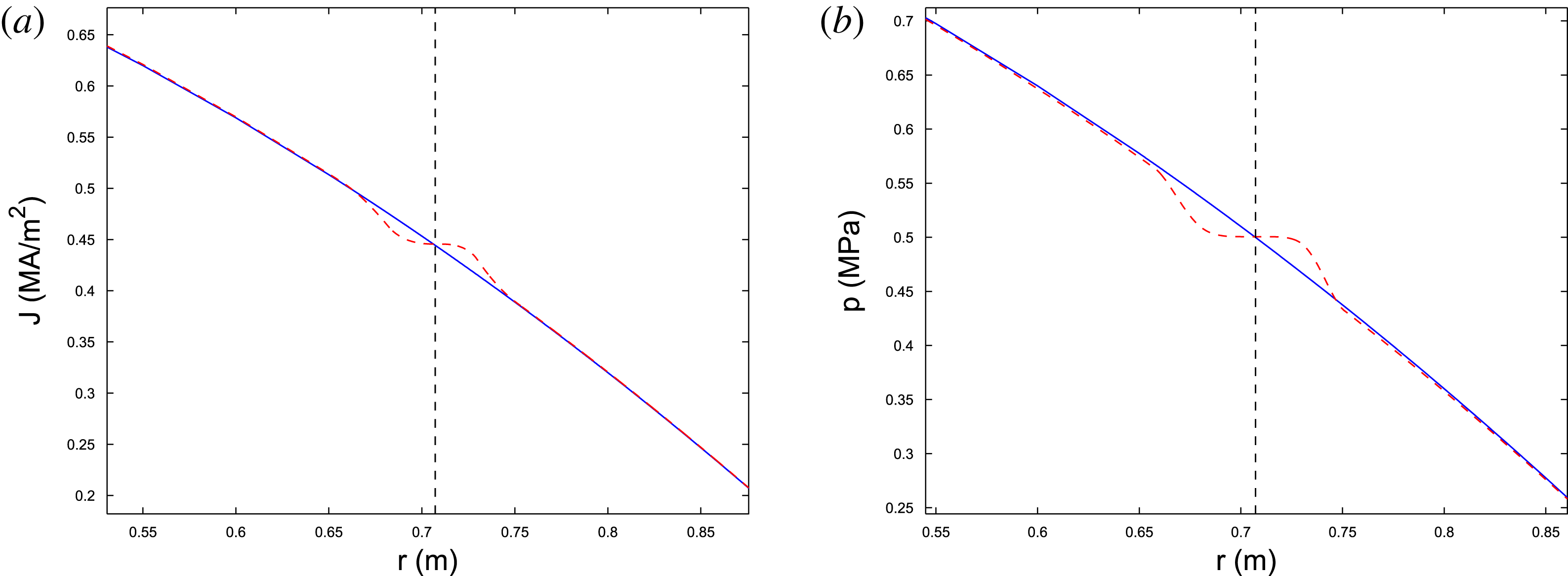
An example of zeroth harmonics of modified profiles thus obtained is shown in figure 5, with the black dashed line representing the position of the resonant surface.
A sample zeroth harmonic modification induced by a finite size island of both (a) current density profile and (b) pressure profile. The solid blue lines show the unperturbed profiles, and the red dashed dot lines stand for the zeroth harmonic of the modified profiles. The resonant surface is represented by the black dashed lines.

7. Perturbed equilibria as marginal stable points for resistive modes
Using the modified current and pressure profile within the island, we can now proceed to the equilibrium equation inside the island 2-D zone. In § 2.2, we have demonstrated that solving for mode structure in the absence of any island is equivalent to searching for a perturbed equilibrium by considering the principal harmonic of equilibrium profiles to have the form:
 $\langle j\rangle _{1}=(\text{d}j_{0}/\text{d}{\it\Psi}_{0}){\it\psi}$
. This is not applicable in the island region, where Fourier decomposition of 2-D profiles should be used. The solutions outside and inside the 2-D zone should be matched at the boundary of this 2-D region. The perturbed equilibrium thus acquired is the mode structure of the corresponding saturated resistive mode and is determined by the condition that there is no jump of the magnetic flux gradient across the resonant surface.
This method avoids singularities in the second-order ODE near the resonant point.
The zeroth harmonic of equilibrium equation (2.11) describes the modified background current density
 $$\begin{eqnarray}\displaystyle \frac{1}{r}\frac{\partial }{\partial r}\left(r\frac{\partial }{\partial r}\langle {\it\Psi}^{\ast }\rangle _{0}\right) & = & \displaystyle -\left\langle \left[1+k^{2}r_{s}^{2}\left(1-\frac{m^{2}}{n^{2}}\right)\right]P+T\right\rangle _{0}\nonumber\\ \displaystyle & & \displaystyle -\,k^{2}(r^{2}-r_{s}^{2})\left(1-\frac{m^{2}}{n^{2}}\right)\langle P\rangle _{0}+2kB_{z},\end{eqnarray}$$
while the principal harmonic describes the perturbed poloidally oscillating current density
 $$\begin{eqnarray}\displaystyle \frac{1}{r}\frac{\partial }{\partial r}\left(r\frac{\partial }{\partial r}{\it\psi}\right) & = & \displaystyle -\left\langle \left[1+k^{2}r_{s}^{2}\left(1-\frac{m^{2}}{n^{2}}\right)\right]P+T\right\rangle _{1}\nonumber\\ \displaystyle & & \displaystyle -\,k^{2}(r^{2}-r_{s}^{2})\left(1-\frac{m^{2}}{n^{2}}\right)\langle P\rangle _{1}+\frac{m^{2}}{r^{2}}{\it\psi}.\end{eqnarray}$$
Note that in order to mimic the toroidal case, the factor
 $1-m^{2}/n^{2}$
(Zakharov Reference Zakharov1978) was introduced, multiplying the curvature term and pressure gradient. It is convenient to define the following notation:
 $$\begin{eqnarray}\displaystyle & \displaystyle j^{\ast }({\it\Psi}^{\ast })\equiv \left[1+k^{2}r_{s}^{2}\left(1-\frac{m^{2}}{n^{2}}\right)\right]P({\it\Psi}^{\ast })+T({\it\Psi}^{\ast }), & \displaystyle\end{eqnarray}$$
 $$\begin{eqnarray}\displaystyle & \displaystyle {\it\delta}j^{\ast }\equiv k^{2}(r^{2}-r_{s}^{2})\left(1-\frac{m^{2}}{n^{2}}\right)P({\it\Psi}^{\ast }). & \displaystyle\end{eqnarray}$$
So that (7.1), (7.2) can be simplified as:
 $$\begin{eqnarray}\displaystyle & \displaystyle \frac{1}{r}\frac{\partial }{\partial r}\left(r\frac{\partial }{\partial r}\langle {\it\Psi}^{\ast }\rangle _{0}\right)=-\langle j^{\ast }\rangle _{0}-\langle {\it\delta}j^{\ast }\rangle _{0}+2kB_{z}, & \displaystyle\end{eqnarray}$$
 $$\begin{eqnarray}\displaystyle & \displaystyle \frac{1}{r}\frac{\partial }{\partial r}\left(r\frac{\partial }{\partial r}{\it\psi}\right)=-\langle j^{\ast }\rangle _{1}-\langle {\it\delta}j^{\ast }\rangle _{1}+\frac{m^{2}}{r^{2}}{\it\psi}. & \displaystyle\end{eqnarray}$$
Here,
 $\langle f\rangle _{0}$
refers to the zeroth harmonic component of function
 $f$
, while
 $\langle f\rangle _{1}$
refers to the principal harmonic
 $m,n$
. The profile of
 $j^{\ast }$
and
 ${\it\delta}j^{\ast }$
are known from § 6. Numerical observation indicates that, with the toroidal
 ${\it\beta}\sim 1\,\%$
, the contribution from
 ${\it\delta}j^{\ast }$
outside the island is more than an order-of-magnitude smaller than
 $j^{\ast }$
due to small factor
 $k^{2}(r^{2}-r_{s}^{2})$
, while in the 2-D zone, it is essential. Outside the 2-D zone, the principal harmonic can be approximated by an ideal linear expression
 $$\begin{eqnarray}\langle j\rangle _{1}=\frac{\text{d}\langle j^{\ast }+{\it\delta}j^{\ast }\rangle _{0}}{\text{d}\langle {\it\Psi}^{\ast }\rangle _{0}}{\it\psi}\simeq \frac{\text{d}\langle j^{\ast }\rangle _{0}}{\text{d}\langle {\it\Psi}^{\ast }\rangle _{0}}{\it\psi},\end{eqnarray}$$
in the linear eigen-equation (4.1). The value and derivatives of the solution are matched at the boundary of the 2-D zone, giving the complete solution across the whole plasma. This method can be applied to any general current and pressure profile to study the nonlinear behaviour of the mode, especially the marginal stable points of the resistive mode.
As an example of the application of this approach, the
 $2/1$
tearing mode in a finite
 ${\it\beta}$
plasma will be studied in the rest of this section. Two marginal stable points will be found, one corresponds to the critical island size beyond which the Glasser effect is overcome, the other corresponds to the saturation size of the island.
The unperturbed equilibrium profile has the following form:
 $$\begin{eqnarray}\displaystyle & \displaystyle j(r)=j(0)\left[(1-f_{2})(1-f_{1})\left(1-\frac{r^{2}}{a^{2}}\right)+(1-f_{2})\left(1-\frac{r^{2}}{a^{2}}\right)^{2}+f_{2}\left(1-\frac{r^{2}}{a^{2}}\right)^{3}\right],\qquad & \displaystyle\end{eqnarray}$$
 $$\begin{eqnarray}\displaystyle & \displaystyle p(r)=p(0)\left(1-\frac{r^{2}}{a^{2}}\right).\qquad & \displaystyle\end{eqnarray}$$
Here,
 $f_{1}$
is chosen to be 0.5 and
 $f_{2}$
is 0.35, the corresponding central safety factor
 $q(0)=1.074$
, edge safety factor
 $q(a)=3$
and
 $2/1$
resonant surface is located at
 $r_{s}=0.776$
. An ideally conducting wall is placed right out of the plasma boundary so that the
 $3/1$
mode is stable. If
 ${\it\beta}$
is negligible, this current profile will give
 ${\it\Delta}^{\prime }=6$
. Now, we consider a pressure profile with central pressure of the plasma to be
 $p(0)=0.5$
, which corresponds to toroidal
 ${\it\beta}=1\,\%$
. This moderate
 ${\it\beta}$
corresponds to a Suydam–Mercier index
 ${\it\nu}=2.275\times 10^{-2}$
. We are primarily interested in the stability rather than actual growth rate of the mode, so we will be looking at the dependence of
 ${\it\Delta}^{\prime }$
on the island size. Here,
 ${\it\Delta}^{\prime }$
is once again defined as
 $$\begin{eqnarray}{\it\Delta}^{\prime }\equiv \frac{{\it\psi}^{\prime }|_{-}^{+}}{{\it\psi}_{s}}.\end{eqnarray}$$
The mode structure is acquired by shooting from both sides of the resonance using the method introduced at the beginning of this section.
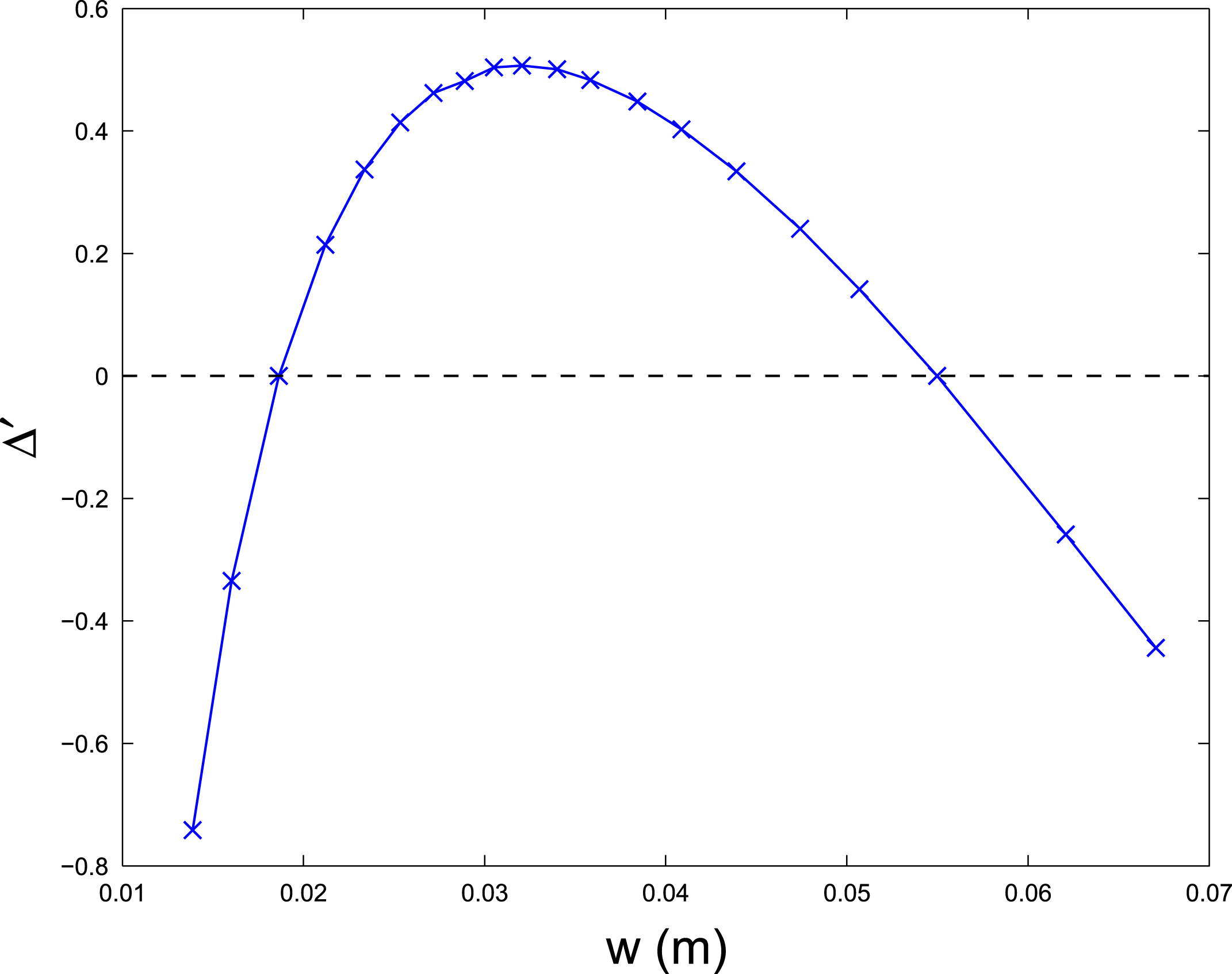
A scan of
 ${\it\Delta}^{\prime }$
of the
 $2/1$
mode for varying island width
 $w$
. Two marginal stable points are evident in the plot. The first represents the critical island width beyond which the stabilizing Glasser effect is overcome, and the resistive mode is linearly stable while nonlinearly unstable. The second represents the saturation point where the plasma reaches a new perturbed equilibrium.

The relationship between
 ${\it\Delta}^{\prime }$
and island width
 $w$
is shown in figure 6. The two marginal stable points are clearly shown in the figure. The first one corresponds to the critical island width where the destabilizing current drive finally balances the stabilizing Glasser effect, and the once linearly stable resistive mode is now nonlinearly unstable. The second marginal stable point corresponds to the saturation level where the plasma reaches a new equilibrium. We notice that the critical island size to overcome the Glasser effect is larger than that given by (5.24) when simply assuming that
 ${\it\Delta}_{\ast }^{\prime }$
is just the
 ${\it\Delta}^{\prime }$
in the zero pressure case. Under this assumption, (5.24) gives the critical island width
 $w_{c}^{\ast }=9.18\times 10^{-3}$
, which is less than half of the actual critical island size, as can be seen from figure 6. The reason for this discrepancy is twofold. The first reason is the fact that finite
 ${\it\beta}$
will also change the ideal mode structure outside the island region, so that
 ${\it\Delta}_{\ast }^{\prime }$
is not the same as
 ${\it\Delta}^{\prime }$
in the no
 ${\it\beta}$
case. The other reason is the profile modification within the island, which is not taken into account in the stability criterion of (5.24). These modifications can have strong impact on the stability of the resistive mode (White Reference White1986; White et al.
Reference White, Gates and Brennan2015).
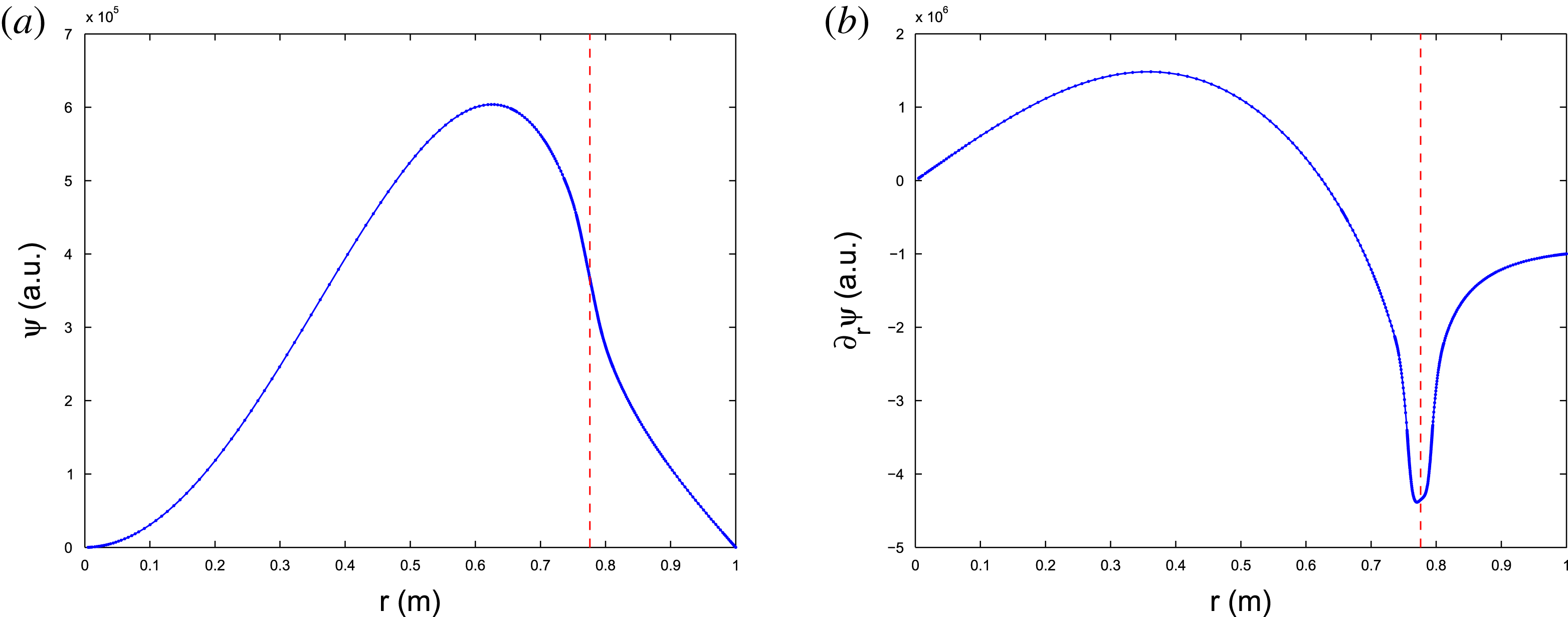
The mode structure at the two marginal stable points is also of interest. We first look at the mode structure at the first marginal stable point which corresponds to the balancing of the Glasser effect. The perturbed helical flux
 ${\it\psi}$
and its radial derivative
 ${\it\psi}^{\prime }$
are shown in figure 7. The position of the resonance is
 $r_{s}=0.776$
, the critical island width is
 $w_{c}=1.864\times 10^{-2}$
with an island asymmetry
 $s=1.031\times 10^{-3}$
. It can be clearly seen from the figure that there is no jump or singularity in either the helical flux or its radial derivative across the whole plasma, and the resistive mode is marginally stable. Thus the plasma is in a new equilibrium at this point.
Although the resistive mode is marginally stable, the perturbed equilibrium state is not, as can be seen from figure 6. Any perturbation to the helical flux, positive or negative, will push the configuration either toward a stable saturated equilibrium or toward the unperturbed configuration with no island.
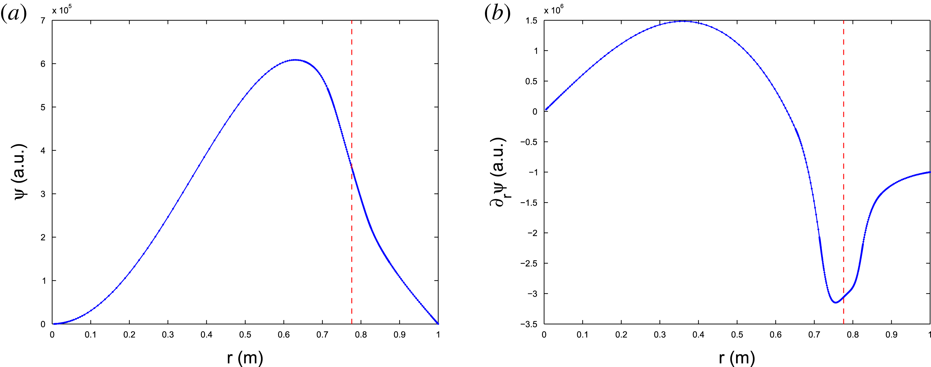
In the former case, the saturation island size is
 $w_{s}=5.498\times 10^{-2}$
with an island asymmetry
 $s=6.406\times 10^{-3}$
. The mode structure at this point is shown in figure 8. Again, there is no jump or singularity in either the helical flux or its radial derivative, and the plasma finally reaches a stable new equilibrium.
A sample
 $2/1$
resistive mode structure at the marginal stable point which corresponds to the balancing of the Glasser effect. There is no jump of derivative or singularity across the whole plasma, and the mode is in a de facto equilibrium. (a) The perturbed helical flux
 ${\it\psi}$
, and (b) the radial derivative of perturbed helical flux
 $\partial _{r}{\it\psi}$
.

Same (a)
 ${\it\psi}$
and (b)
 $\partial _{r}{\it\psi}$
profiles for the case of the island saturation. There is no jump of the derivative or singularity across the whole plasma, and the mode is in a new stable perturbed equilibrium.

8. Limitations of a simplistic quasilinear treatment
One simplified approach to consider the quasilinear equilibria is the use of the linear ideal mode equation with current density and pressure profiles corresponding to their zeroth harmonics in the configuration perturbed by the island.
Here, we compare this simplistic approach with the perturbed equilibrium of § 7. It will be found that this simplified quasilinear treatment cannot catch the mode structure within the island region accurately. Moreover, it will be shown that such a treatment overestimates the instability, e.g. it yields a positive growth rate even when the plasma is in a saturated equilibrium.
We will present both the zero
 ${\it\beta}$
case and finite
 ${\it\beta}$
cases. The growth rates for equilibrium with and without an island for both cases will be shown. The simplistic quasilinear treatment is carried out without scaling the independent coordinate in the resistive inner region as opposed to the traditional asymptotic method. This method was first proposed by Furukawa, Tokuda & Zheng (Reference Furukawa, Tokuda and Zheng2010) to treat linear resistive instabilities. We are extending its usage to treat the finite size island.
Both cases have the following common parameters. We take a minor radius
 $a=1$
, major radius
 $R=10$
and toroidal field
 $B_{t}=10$
. The current and pressure profiles for both cases are the same as in § 7, except for the finite
 ${\it\beta}$
case where the value
 ${\it\beta}=0.4\,\%$
was used. The edge safety factor
 $q(a)=3$
, and the
 $2/1$
resonant surface is at
 $r_{s}=0.776$
. An ideally conducting wall is placed outside the plasma boundary so that the
 $3/1$
mode is stable.
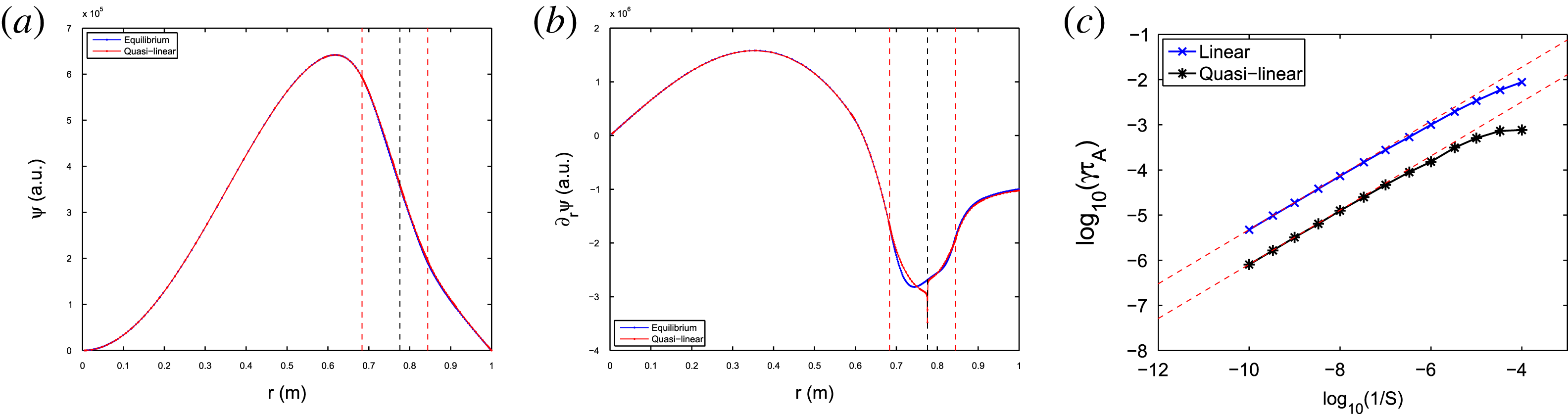
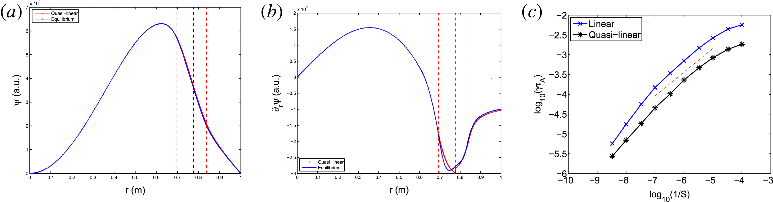
Figure 9 shows the zero
 ${\it\beta}$
mode structure calculated by both simplistic and perturbed equilibrium methods at the saturation point. The red line represents the quasilinear result and the blue line represents the perturbed equilibrium. It can be seen that the quasilinear mode structure deviates from the perturbed equilibrium within the island. The linear and quasilinear growth rate as a function of resistivity are shown in figure 9(c), with
 ${\it\tau}_{A}\equiv R/v_{A}$
the Alfvén time,
 ${\it\tau}_{{\it\eta}}\equiv a^{2}/\bar{{\it\eta}}$
the resistive time and
 $S\equiv {\it\tau}_{{\it\eta}}/{\it\tau}_{A}$
the Lundquist number. It can be seen that at low resistivity, the growth rate agrees well with the asymptotic
 $3/5$
prediction, while at higher resistivity the asymptotic treatment fails. It can also be seen that a simple quasilinear treatment is not accurate as it predicts a positive growth rate when the new equilibrium has been reached.
A comparison between (a) a perturbed helical flux
 ${\it\psi}$
, and (b) its radial gradient
 ${\it\psi}^{\prime }$
for simplistic quasilinear (red curve) and perturbed (blue) equilibria of
 $2/1$
tearing mode for
 ${\it\beta}=0$
and
 $S=10^{7}$
. The black dashed line denotes the location of the resonant surface, and the red dashed lines represent the boundaries of the island. Additionally, the linear (blue cross) and quasilinear (black star) growth rate as a function of resistivity are shown in (c), with the red dashed line representing the
 $3/5$
law predicted by asymptotic theory. It can be seen that the presence of the island does not affect the growth rate in the simplistic approach.

The same comparison for the
 ${\it\beta}=0.4\,\%$
case. All the other parameters are identical to the previous
 ${\it\beta}=0$
case. (a) The helical flux
 ${\it\psi}$
, and (b) its radial derivative
 ${\it\psi}^{\prime }$
and (c) the growth rates of resistive mode in unperturbed and perturbed equilibria as erroneously predicted by the simplistic quasilinear method in the presence of an island.

Similarly, figure 10 shows the comparison for the
 ${\it\beta}=0.4\,\%$
case. Once again, the quasilinear mode structure deviates from the perturbed equilibrium within the island 2-D region, and the simplistic method predicts an instability for the saturated configuration.
These two examples demonstrate that the simple quasilinear treatment is not suitable for assessing the resistive stability of magnetically perturbed configurations with islands.
9. Conclusion and discussion
In light of the various difficulties faced by the traditional asymptotic matching technique, an alternative, perturbed equilibrium method is introduced in this paper to study both the linear and nonlinear stability of the tearing or resistive kink mode for a finite
 ${\it\beta}$
plasma. The core idea of this method is to view the mode structure as a perturbed equilibrium with prescribed current density and pressure profiles in the island zone, and extraction of the Fourier harmonics of the current density using the magnetic geometry of the 2-D zone near the island.
For linear mode calculations, a new mathematical method for proper extraction of the small and large solutions without numerical difficulties was presented for both zero and finite
 ${\it\beta}$
cases. These solutions determine the stability criterion, as well as providing an accurate description of the linear mode structure. The origin of the Glasser effect and its mitigation were briefly discussed. Our analysis reveals a fundamental problem in the applicability of this and any other asymptotic methods due to their requirement for excessive accuracy of the configuration parameters. The perturbed equilibrium method of this paper does not suffer such a problem.
The perturbed equilibrium approach was compared with a simplistic quasilinear treatment which solves the linear equation using the zeroth harmonic of the current and pressure modifications. It is found that, within the island zone, this method is not applicable as it predicts instability even for a saturated equilibrium.
Presented here for a cylindrical case, the perturbed equilibrium technique can be extended to the toroidal perturbed equilibrium with minor modifications. Two more effects may be taken into account in the future which may affect the stability and saturation of the resistive mode. The first corresponds to non-flat profiles inside the island, which recently have been the subject of discussion due to the thermal instability caused by island cooling (Gates & Delgato-Aparicio Reference Gates and Delgato-Aparicio2012; White et al. Reference White, Gates and Brennan2015). The profiles described in § 6 take into account this potential modification. Also, external current drive and bootstrap current contribution can be included in the model. The other factor is the presence of background shear flow. Differential rotation has generally a stabilizing effect on the growth of magnetic islands. However, it has been reported that shear flow has only limited impact on the stability of magnetic islands for a fully relaxed equilibrium (Waelbroeck, Fitzpatrick & Grasso Reference Waelbroeck, Fitzpatrick and Grasso2007). A potentially interesting case for future considerations is the situation when the differential rotation is fast enough to match the local poloidal Alfvén speed, so that singular currents develop at those Alfvén resonances (Wang et al. Reference Wang, Bhattacharjee, Ma, Ren, Hegna and Callen1998).
Acknowledgements
The authors thank A. H. Glasser, R. B. White, A. Bhattacharjee, X.-G. Wang and Q. Teng for fruitful discussion. This work is partially supported by US DoE contract no. DE-AC02-09-CH11466, the National Natural Science Foundation of China under grant no. 11261140326, Chines National Fusion Project for ITER under grant no. 2014GB107004, and the China Scholarship Council.