2.1 Primary instability

In his review article, Bippes (Reference Bippes1999) reported several experiments, conducted over a period of years at DLR (e.g. Deyhle & Bippes Reference Deyhle and Bippes1996), making use of different models and placed in several facilities in order to see the effect of model geometry and tunnel free stream turbulence on instability development. It was found that the model leading edge radius influences the attachment line instability while the curvature of the surface has a stabilising effect when convex and a destabilising effect when concave due to the generation of Görtler vortices. The free stream turbulence level instead changes the type of the amplified crossflow instability modes: in lower turbulence tunnels (with a free stream turbulence intensity related to the free stream velocity of $Tu/U_{\infty }<0.15\,\%$ ) stationary crossflow waves are observed while, in higher turbulence facilities, travelling modes take place and dominate the transition scenario.

Similar results were recently shown through the extensive measurements performed by Downs & White (Reference Downs and White2013), by carefully modifying and measuring the turbulence intensity of the KSWT facility at TAMU by means of turbulence screens. Their results confirm the effectiveness of surface roughness in forcing the primary stationary modes and the capability of free stream turbulence to enhance primary travelling instabilities, adding that the latter are also highly sensitive to the surface roughness.

The studies carried at ASU concentrated mainly on the effect of surface roughness on the stability of the boundary layer and led to significant conclusions: Reibert et al. (Reference Reibert, Saric, Carrillo and Chapman1996) measured several stationary waves in the boundary layer developing on a $45^{\circ }$ swept wing featuring a laminar airfoil at chord Reynolds number of $2.4\times 10^{6}$ . Towards simplifying the flow arrangement and to facilitate comparison with numerical results, they made use of small roughness elements (cylindrical rub-on transfers with a diameter of 3.7 mm and height of 6  ${\rm\mu}$ m) placed at the model leading edge region. The roughness elements were spaced along the spanwise direction at distances matching the wavelength predicted by linear stability theory (LST) for the most amplified stationary mode. The discrete roughness elements fixed the wavelength of the amplified mode leading to a more uniform transition pattern compared to the unforced case. The spatial amplification factors of the stationary vortices were reported featuring a monotonic growth till a given saturation amplitude prior to the onset of transition. In the same study, the flow configuration was forced by placing the roughness elements at three times the wavelength of the naturally dominant mode. This case showed again the naturally most amplified mode to dominate the transition process but showed also that all the higher harmonics of the forced mode (i.e. shorter wavelength modes) were amplified. In contrast, no lower harmonics were observed in both the performed tests. Moreover they showed that if stationary modes undergo amplitude saturation, then the forcing amplitude does not modify the transition process.

These observations were at the base of the study done by Saric et al. (Reference Saric, Carrillo and Reibert1998) and White & Saric (Reference White and Saric2000), centred on the idea of forcing a subcritical mode, which is a mode with a wavelength smaller than that of the most amplified mode. The experiment of Saric et al. (Reference Saric, Carrillo and Reibert1998), done at the same flow conditions as the one of Reibert et al. (Reference Reibert, Saric, Carrillo and Chapman1996), led to the remarkable conclusion that subcritical forcing can delay transition to turbulence for stationary crossflow instability boundary layers. This transition control strategy has been followed by several other experimental (Downs & White Reference Downs and White2013; Serpieri & Kotsonis Reference Serpieri and Kotsonis2015b ), theoretical (Malik et al. Reference Malik, Li, Choudhari and Chang1999) and numerical (Wassermann & Kloker Reference Wassermann and Kloker2002; Hosseini et al. Reference Hosseini, Tempelmann, Hanifi and Henningson2013) studies. Transition delay by this technique has not been always observed (Downs & White Reference Downs and White2013) and would need further investigation.

Radeztsky, Reibert & Saric (Reference Radeztsky, Reibert and Saric1999) demonstrated the effect of discrete surface roughness on transition location. They performed a careful study of the geometrical parameters (width and height) of the roughness elements, showing promotion of transition for taller roughness elements of diameter up to 0.08 times the mode wavelength. For larger diameters, increasing the height of the roughness elements did not have an effect on the transition onset. Additionally, they showed relative insensitivity of the transition process to strong and broadband acoustic forcing, in agreement with the work of Deyhle & Bippes (Reference Deyhle and Bippes1996).

Tempelmann et al. (Reference Tempelmann, Schrader, Hanifi, Brandt and Henningson2012) studied the boundary layer receptivity to surface roughness by means of parabolised stability equations (PSE) and adjoint PSE together with DNS. They commented on the discrepancies with the experimental results of Reibert et al. (Reference Reibert, Saric, Carrillo and Chapman1996) pointing at possible small imperfections in the application of roughness elements on the model surface (which is very likely in laboratory conditions given the micrometric size of these elements). The problem of receptivity to surface roughness was further investigated by Kurz & Kloker (Reference Kurz and Kloker2014) in a following DNS study. They found that the amplitude of the fundamental stationary mode scales linearly with the roughness height only when the roughness array features null spanwise-averaged shape and flow blockage.

2.2 Secondary instability

In his study on the stability of a swept cylinder, Poll (Reference Poll1985) measured high-frequency boundary layer fluctuations superimposed on the primary crossflow instability mode. These were reported also in the swept wing experiments by Kohama, Saric & Hoos (Reference Kohama, Saric and Hoos1991) and identified as a secondary instability mechanism acting on the boundary layer, modified by the primary stationary crossflow modes. Since these early works, efforts in revealing the nature and the evolution of the crossflow secondary instability have intensified.

Malik et al. (Reference Malik, Li, Choudhari and Chang1999), following the work of Malik, Li & Chang (Reference Malik, Li and Chang1994) on a Hiemenz flow, exploited linear and nonlinear parabolised stability equations (PSE and NPSE) to assess the evolution of the primary instabilities as well as a temporal two-dimensional eigenvalue problem to study the secondary instability for the flow case of the ASU experiments (Reibert et al. Reference Reibert, Saric, Carrillo and Chapman1996). Under the assumption that the secondary modes are of a convective nature (see also the theoretical efforts of Fischer & Dallmann (Reference Fischer and Dallmann1991), Lingwood (Reference Lingwood1997), Janke & Balakumar (Reference Janke and Balakumar2000), Koch et al. (Reference Koch, Bertolotti, Stolte and Hein2000) and Koch (Reference Koch2002)), they used Gaster’s transformation to track the modes spatial evolution, finding good agreement with the experimental results. Another key contribution from the work of Malik et al. (Reference Malik, Li, Choudhari and Chang1999) is the classification of the secondary instability into two main modes. The first is the type-I mode, related to the streamwise flow velocity gradient along the spanwise direction (usually $z$ , from which this mode is also referred to as the z-mode) located at the outer side of the upwelling region of the primary crossflow vortex and characterised by higher energy and lower frequencies. The second is the type-II mode, or y-mode, that is located on the top of the primary vortices where the streamwise velocity wall-normal ( $y$ ) gradients are larger. This mode features lower energy but higher frequencies. As a last outcome of this study, a transition estimation criterion based on secondary instability amplification was presented, showing good correlation with the transition locations measured by Reibert et al. (Reference Reibert, Saric, Carrillo and Chapman1996).

Haynes & Reed (Reference Haynes and Reed2000) used linear and nonlinear PSEs as well as LST to investigate the boundary layer experimentally measured by Reibert et al. (Reference Reibert, Saric, Carrillo and Chapman1996). Their results are in very good agreement with the experimental data. Furthermore, the study highlighted the importance of including nonlinear terms and surface curvature. Convex surfaces have a stabilising effect on the primary vortices and as such, enhance their saturation and the occurrence of secondary modes.

Floquet analysis was used by Fischer & Dallmann (Reference Fischer and Dallmann1991) and Janke & Balakumar (Reference Janke and Balakumar2000) to inspect the secondary stability of the CF vortices of the DLR experiment (Deyhle & Bippes Reference Deyhle and Bippes1996) (in the second study, the secondary instability of a Hiemenz flow boundary layer was also considered). One of the main outcomes from these studies is the investigation of the low-frequency type-III mode. This mode refers to the interactions between primary stationary and primary travelling modes and therefore its relevance in the transition pattern depends on the free stream turbulence level (Högberg & Henningson Reference Högberg and Henningson1998; Downs & White Reference Downs and White2013).

White & Saric (Reference White and Saric2005) dedicated a detailed experimental investigation to the secondary instability mechanisms and sensitivity to different base flow cases. Hot-wire measurements of velocity fluctuations, corresponding to the secondary instability, were extracted for a chord Reynolds number flow of $Re=2.4\times 10^{6}$ under critical stationary mode forcing. Following previous works, micron-sized roughness elements were placed at the leading edge region spaced at the wavelength of the most amplified mode. In this study, the different secondary instability modes were detected and their appearance and sudden growth identified as the cause of turbulent breakdown. The conditions under which the type-II mode arises and reaches higher energies are those of supercritical forcing (same roughness spacing as the $Re=2.4\times 10^{6}$ case but Reynolds number increased to $Re=2.8\times 10^{6}$ ) where the spanwise shear and hence type-I modes are mitigated (see also Hosseini et al. Reference Hosseini, Tempelmann, Hanifi and Henningson2013). Furthermore, the influence of increased free stream turbulence and of acoustic forcing on the transition scenario were also investigated but required further dedicated efforts which came later with the already mentioned study of Downs & White (Reference Downs and White2013).

The first spatial DNS study on the development of secondary instability modes over the primary stationary vortices was performed by Högberg & Henningson (Reference Högberg and Henningson1998). They studied the evolution of a Falkner–Skan–Cooke boundary layer subject to fixed steady primary forcing and random unsteady excitation of the secondary instability via the use of volume body forces. The location of the unsteady volume forces changed the nature of the amplified modes: a more upstream forcing gave rise to lower-frequency type-III modes, while a more downstream forcing, close to the location of primary saturation, led to the triggering of the aforementioned high-frequency type-I modes. The latter mode showed much larger growth rates than the low-frequency type-III mode.

Two later DNS investigations by Wassermann & Kloker (Reference Wassermann and Kloker2002, Reference Wassermann and Kloker2003) further described the secondary instability modes developing around stationary and travelling CF vortices, respectively. In these works, the type-I secondary instability vortices are visualised and described as a sequence of corotating helicoidal structures superimposed on the upwelling region of the primary vortices and convecting downstream. The axes of these structures form a considerable angle with the one of the primary waves and the spinning direction of the two modes is opposite. An interesting outcome of the simulations of Wassermann & Kloker (Reference Wassermann and Kloker2002, Reference Wassermann and Kloker2003) is that, when the unsteady disturbance that triggers the secondary modes is switched off, the associated structures are advected downstream, thus confirming the findings of Kawakami et al. (Reference Kawakami, Kohama and Okutsu1999) and Koch (Reference Koch2002) regarding the convective nature of these instability modes.

Another relevant investigation on the secondary instability of stationary and travelling primary CF vortices was reported by Bonfigli & Kloker (Reference Bonfigli and Kloker2007). In this study the authors used spatial DNS and secondary linear stability theory (SLST), the latter previously applied by Fischer & Dallmann (Reference Fischer and Dallmann1991), Malik et al. (Reference Malik, Li and Chang1994, Reference Malik, Li, Choudhari and Chang1999), Janke & Balakumar (Reference Janke and Balakumar2000) and Koch (Reference Koch2002). The two techniques showed good agreement in terms of eigenfunctions and growth rates when the DNS analysis is tuned to the simplified base flow of the SLST. The two techniques captured the structures related to the type-I and type-III instabilities, whereas DNS did not show amplification of the type-II instability predicted by SLST. For the analysis of the travelling primary CF instability, with no stationary modes considered, destabilisation of the type-III mode is not reported. This is expected given that this mode is generated by the spanwise modulation of the primary travelling waves (see also Fischer & Dallmann Reference Fischer and Dallmann1991; Högberg & Henningson Reference Högberg and Henningson1998; Janke & Balakumar Reference Janke and Balakumar2000) caused by the stationary CF vortices. One more important outcome from the work of Bonfigli & Kloker (Reference Bonfigli and Kloker2007) relates to the nature of type-I and type-II modes. The behaviour and location of these modes associates them to instabilities of the Kelvin–Helmholtz type.

The possibility of experimentally confirming the outcomes of these theoretical and numerical investigations on the spatio-temporal development of the secondary instability has been so far limited. This is attributed to the inherent features of the technique mainly used in wind tunnel tests: single or double-wire hot-wire probes. Hot-wires, although being very accurate for this type of experiment, are a point measurement technique and as such cannot infer any information regarding the spatio-temporal evolution of the unsteady structures described by Högberg & Henningson (Reference Högberg and Henningson1998), Malik et al. (Reference Malik, Li and Chang1994, Reference Malik, Li, Choudhari and Chang1999) and Wassermann & Kloker (Reference Wassermann and Kloker2002, Reference Wassermann and Kloker2003), Bonfigli & Kloker (Reference Bonfigli and Kloker2007).

A successful attempt to overcome this limitation was performed by Kawakami et al. (Reference Kawakami, Kohama and Okutsu1999), who inferred the spatio-temporal evolution of the secondary instabilities in an experimental framework. Although the technique they used was still based on hot-wire measurements, they forced the secondary modes at their respective frequencies by applying unsteady blowing and suction in the boundary layer undergoing primary mode saturation, similarly to what done in their numerical framework by Högberg & Henningson (Reference Högberg and Henningson1998). By correlating the wire signal at the several phases of the actuation, they were able to reconstruct the shape, projected in two-dimensional planes, the direction and the velocity by which the secondary type-I waves and the primary travelling lower-frequency type-III modes are evolving in the boundary layer.

Similarly to Kawakami et al. (Reference Kawakami, Kohama and Okutsu1999), Chernoray et al. (Reference Chernoray, Dovgal, Kozlov and Löfdahl2005) performed phase locked hot-wire measurements on the secondary instability of streamwise vortices in a swept wing boundary layer. These vortices were not generated by crossflow instability mechanisms, but rather directly caused by large roughness elements or localised continuous suction and were subsequently subject to the crossflow. Despite these differences, their measurements encompassed full volumes and hence led to the description of the three-dimensional organisation and streamwise evolution of the streamwise vortices and their instability.

Simultaneous multipoint measurements have been performed using surface mounted hot-film sensors (Glauser et al. Reference Glauser, Saric, Chapman and Reibert2014). However, the sensors were located at the wall and the region of the flow field that was investigated was quite small and not in the zone of the boundary layer mainly influenced by the secondary instability. Despite this, the simultaneous use of multiple sensors allowed the study of the spatial coherence of the vortical structures by means of POD. A correlation between the first and second POD modes with the primary travelling crossflow mode and the secondary instability, respectively, was proposed for a transition prediction criterion.

It is evident from previous work that the role of the secondary instability is catalytic in the swept wing transition scenario. Additionally, due to limitations of measurement techniques, the only information on the spatio-temporal characteristics of these modes is available from numerical simulations, theoretical investigations or phase locked measurements. All these approaches though imply artificially imposed unsteady forcing at arbitrary amplitude, which requires opportune calibration.

2.3 Present work

The present study was performed at the Delft University of Technology Aerodynamics laboratories towards experimentally investigating the primary and secondary crossflow instability. A $45^{\circ }$ swept wing model was designed following the guidelines set by the ASU and TAMU campaigns (for details see Serpieri & Kotsonis Reference Serpieri and Kotsonis2015a ) and installed in the low turbulence tunnel (LTT). A preliminary flow visualisation campaign was performed to assess the flow evolution and its main stability characteristics (Serpieri & Kotsonis Reference Serpieri and Kotsonis2015b ). These were also inspected by means of LST applied to numerical solutions of the developing boundary layer. Boundary layer measurements by means of hot-wire anemometers and three-component three-dimensional particle image velocimetry (tomographic or tomo-PIV) were performed. Hot-wire scans covered a wider region in space and, given their extremely high temporal resolution, allowed the spectral content of the unsteady fluctuations to be inferred. The tomo-PIV investigation was instead confined to the boundary layer region where the primary stationary waves saturate. Having simultaneous volumetric field data allowed the deployment of powerful data reduction and mode identification techniques such as POD. These techniques greatly enhance the identification and description of the temporal and spatial organisation of the unsteady modes in an experimental framework under natural flow conditions.

The experimental set-ups of the flow visualisation, hot-wire and tomo-PIV experiments are introduced in § 3. The linear stability analysis is presented in § 4. Section 5 is dedicated to the discussion of the boundary layer primary stationary instability. The outcomes of the investigation of the secondary instability are presented in § 6. The conclusions of this study are in § 7.

3.1 Swept wing model, wind tunnel facility and test conditions

The model used in the current investigation is a swept wing of approximately 1.25 m in span ( $b$ ) with a 1.27 m chord in the free stream direction ( $c_{X}$ ). The sweep angle ( ${\it\Lambda}$ ) is $45^{\circ }$ . The model is made of fibreglass with a very smooth polished surface, featuring a measured value of surface roughness standard deviation of $R_{q}=0.20~{\rm\mu}$ m. The airfoil used is an in-house modified version of the NACA 66018 shape that was named 66018M3J and features a small leading edge radius of approximately 1 % of the chord in order to avoid attachment line instability (Poll Reference Poll1985; Bippes Reference Bippes1999). Until approximately 70 % of the chord, the airfoil shows accelerating flow when at zero incidence, and has no concave surfaces to avoid the amplification of Tollmien–Schlichting (TS) waves and of Görtler vortices, respectively. The airfoil used is shown in figure 1 together with the NACA 66018 on which it was based. It must be stressed that the wing section is presented along the normal to the leading edge direction.

Figure 1.

The 66018M3J airfoil used in the present work and comparison with the NACA 66018. Wing sections orthogonal to the leading edge direction.

The wind tunnel where the experiments were performed is the TU Delft LTT facility. This is a closed-loop low turbulence subsonic tunnel with a test section of $1.25~\text{m}\times 1.80~\text{m}\times 2.6~\text{m}$ in height, width and length, respectively. The tunnel is furnished with seven anti-turbulence screens and has a contraction ratio of $17:1$ . Turbulence intensity was measured in an empty test section with a single hot-wire sensor at approximately the conditions of the experiment. The acquired signal was bandpass filtered between 2 and 5000 Hz. At the free stream velocity $U_{\infty }=24~\text{m}~\text{s}^{-1}$ the turbulence intensity was found to be $Tu/U_{\infty }=0.07\,\%$ . This value is low enough to observe stationary crossflow waves (Bippes Reference Bippes1999; Downs & White Reference Downs and White2013). The background acoustic emission of the tunnel, although considerable, is not relevant to the transition scenario of this type of flow (Deyhle & Bippes Reference Deyhle and Bippes1996; Radeztsky et al. Reference Radeztsky, Reibert and Saric1999; White & Saric Reference White and Saric2005).

The experiment was performed at Mach number $M=0.075$ ( $U_{\infty }=25.6~\text{m}~\text{s}^{-1}$ ) and Reynolds number $Re=2.17\times 10^{6}$ (based on the free stream velocity and streamwise chord) and at incidence angle of ${\it\alpha}=3^{\circ }$ . The flow over the wing pressure side was investigated. The boundary layer over the wing suction side was forced to a turbulent state close to the leading edge using a tripping wire in order to avoid any unsteady flow separation influencing the measurements on the pressure side.

Figure 2.

Pressure coefficient distribution on the wing pressure side measured by two arrays of 46 pressure taps placed at the 25 and 75 % of the wing span (300 mm from top and bottom wind tunnel wall respectively) at ${\it\alpha}=3^{\circ }$ and $Re=2.17\times 10^{6}$ .

As described in a preliminary work by the authors (Serpieri & Kotsonis Reference Serpieri and Kotsonis2015a ), as well as suggested by Saric et al. (Reference Saric, Reed and White2003), conditions of infinite span swept wing are necessary in order to capture the fundamental features of crossflow-dominated transition. To achieve this condition, the swept wing model used must be able to feature a spanwise-invariant pressure distribution and flow field in the measurement region. In the characterisation work (Serpieri & Kotsonis Reference Serpieri and Kotsonis2015a ), three-dimensional contoured wall liners based on the inviscid streamlines (as done also by e.g. Deyhle & Bippes Reference Deyhle and Bippes1996; Reibert et al. Reference Reibert, Saric, Carrillo and Chapman1996; Radeztsky et al. Reference Radeztsky, Reibert and Saric1999; White & Saric Reference White and Saric2005) were designed and used for the case of zero incidence angle. Comparison of pressure distributions with and without liners showed similar results, suggesting that the wing aspect ratio is sufficient to ensure spanwise invariance even in the absence of wall conditioning. For the present experiment (incidence of ${\it\alpha}=3^{\circ }$ ) the invariance of the flow along the leading edge direction was assessed without the use of liners. Two arrays of 46 streamwise-oriented pressure taps were integrated in the model at approximately 25 and 75 % of the span (300 mm from the tunnel walls). The measured pressure coefficient, for the experiment condition, over the wing pressure side is shown in figure 2. The pressure distributions show a high degree of uniformity without the contoured liners. Furthermore, it is worth noting that, for this flow configuration, the pressure minimum point is at $X/c_{X}=0.63$ and thus far downstream of the transition location, as will be shown later. This is a necessary condition for studies on CF instability as it produces boundary layers stable to TS modes.

Natural transition pertaining to swept wings manifests as a result of the amplification of a narrow band of crossflow modes. Within the band, small variations in spanwise wavelength can compromise the measurement and interpretation of the developing flow field. It becomes therefore important to fix the dominant mode wavelength in order to enhance the uniformity of the boundary layer. Towards this goal, the technique used by Reibert et al. (Reference Reibert, Saric, Carrillo and Chapman1996) was followed in this work. The primary mode was fixed by forcing a known spanwise wavelength using micron-sized roughness elements. A sequence of small cylindrical elements (rub-on transfers used for etch masking of printed circuit boards) was installed on the model surface close to the leading edge ( $X/c_{X}=0.025$ ). These forcing elements have a diameter of $d=2.8$  mm and an average height of $k=10~{\rm\mu}\text{m}$ . They were installed with a spacing along the leading edge direction ( $z$ ) of 9 mm. The selected spacing corresponds to the wavelength of the most amplified stationary mode for these conditions according to LST predictions (§ 4) and preliminary flow visualisation studies (Serpieri & Kotsonis Reference Serpieri and Kotsonis2015a ). This forced wavelength will be henceforth denoted with the symbol: ${\it\lambda}_{z}^{F}$ . The performed LST analysis indicates that the position of the roughness element array is located slightly upstream of the neutral instability location for the the 9 mm stationary mode (§ 4).

3.2 Coordinate systems

Due to the complexity of the swept wing geometry and the multitude of measurement techniques used in this study, a rigorous definition of the coordinate systems and of the velocity components is necessary towards correct interpretation of results. The used systems and respective notations are presented in figure 3. Firstly, the wing un-swept coordinate system is introduced and defined with the upper case letters $XYZ$ . It is aligned with the wing chords plane and the velocity components along this coordinate system are indicated with upper case letters $UVW$ .

Figure 3.

Schematic of the model and definition of the un-swept ( $XYZ$ ), the swept ( $xyz$ ) and the local tangential ( $x_{t}y_{t}z_{t}$ ) reference systems. The chord along $X$ is defined with $c_{X}$ and shown with a black dashed line while the chord along $x$ , defined with $c$ , is plotted with a white dashed line.

The swept wing model is placed at an incidence angle of ${\it\alpha}=3^{\circ }$ and, as such, the wind tunnel reference system does not coincide with the un-swept wing coordinates. The velocity components along the wind tunnel reference system are denoted with upper case letters and the subscript ( $_{\infty }$ ), with $U_{\infty }$ being the free stream velocity.

In figure 3 the swept wing reference system is plotted in grey and is such that its $x$  axis is orthogonal to the wing leading edge direction, with $z$ parallel to it (both these axes lie in the chord plane) and $y$ coincides with the un-swept $Y$ direction. Rotation of ${\it\Lambda}=45^{\circ }$ about the $Y$ axis transforms the $XYZ$ system of coordinates to the swept $xyz$ system. Note that in existing literature, some ambiguity with the definition of swept and un-swept exists (see for instance White & Saric Reference White and Saric2005; Tempelmann et al. Reference Tempelmann, Schrader, Hanifi, Brandt and Henningson2012). In this study the definition of White & Saric (Reference White and Saric2005) is used. The velocity components in this system of coordinates are indicated with the lower case letters $uvw$ . The origins of both the $XYZ$ and $xyz$ systems are at the wing leading edge at the mid-span location. In the schematic, the chords in the $XYZ$ ( $c_{X}$ ) and $xyz$ ( $c$ ) systems are indicated with black and white dashed lines respectively. $X/c_{X}$ is used to define the streamwise measurement station as the HWA traverses were mainly along $X$ and at constant $Z$ (centred at $Z=0$ ). For the LST, the streamwise station is defined with $x/c$ as the formulation of the problem is in the swept wing coordinate system. The two definitions of the chordwise locations are equivalent given the semi-infinite swept wing flow assumption.

One other coordinate system is the local tangential system where the definition of tangential is simplified as it implies only the surface curvature along the $X$ direction. The system is such that the $x_{t}$ axis is aligned with the local surface tangent, the $y_{t}$ is the wall-normal direction and $z_{t}$ coincides with the $Z$ axis.

Finally, the reference system of the primary stationary CF vortices is introduced as $X_{W}Y_{W}Z_{W}$ . A more detailed description of this coordinate system will be given in the next sections.

3.3 Non-dimensionalisation

As evident by the previous discussion, the problem of transition in three-dimensional boundary layers, pertinent to swept wings, is of a complex nature. The multitude of length scales, time scales, measurement techniques and coordinate systems imposes an intriguing problem regarding scaling of the measured variables. Typical for boundary layer flows, a Reynolds-based scaling approach is sought. In such an approach, a reference velocity and reference length are needed. While the free stream velocity is a straightforward choice, the choice for the reference length is, in this case, problematic as no one single parameter can be chosen that can describe the observed phenomena in a consistent and meaningful manner. Possible choices would be the chord of the swept wing, thickness of the boundary layer or spacing of the discrete roughness elements. Choice of chord would lead to inherent inconsistencies with the scales of the investigated primary CF mode, since the latter are locked by the discrete roughness elements. Choice of boundary layer thickness would lead to the collapse of the approximately self-similar laminar boundary layer when comparisons at several chord stations are reported. This choice is not effective in showing the growth of the stationary modes. Finally, choice of the roughness elements spacing as scaling length would lead to inconsistencies between the swept and the stationary CF vortices coordinate systems.

Due to the previous considerations, the choice of using dimensional values for the spatial coordinates is made in this work. This is consistent with several previous investigations of this type of flow (Bippes Reference Bippes1999; Saric et al. Reference Saric, Reed and White2003; White & Saric Reference White and Saric2005; Downs & White Reference Downs and White2013). It should be noted that the streamwise chord ( $c_{X}$ ) is used throughout as the scaling length for the definition of the Reynolds ( $Re=c_{X}U_{\infty }/{\it\nu}$ ) and Strouhal ( $St=fc_{X}/U_{\infty }$ ) numbers.

3.4 Flow visualisation

Flow visualisation was performed by application of a fluorescent mineral oil on the model surface. The applied mixture consists of paraffin oil (Shell Ondina), petroleum and fluorescent mineral pigments in customised ratios according to the tested velocity regime and flow temperature. In this experiment, the mixture was carefully applied on the model surface in a homogeneous manner, taking care to omit the leading edge region in order not to influence the inception of crossflow instability. Illumination was provided by an ultraviolet (UV) lamp and a digital camera equipped with UV filters was used for imaging.

The distribution of wall shear stresses due to the developing flow are indicated by the formation of patterns in the oil. Areas of intense light emission indicate accumulation of oil which denotes low shear stresses. In contrast, darker areas are formed due to elimination of the oil caused by high shear forces. The primary features elucidated by the technique are the laminar–turbulent transition front and its location. Moreover, quantitative information is also accessible via this technique, such as the spacing (spanwise wavelength) of the developing crossflow modes.

3.5 Hot-wire anemometry

Hot-wire measurements were performed with a single-wire boundary layer probe (Dantec Dynamics P15). A second single-wire probe (Dantec Dynamics P11) performed simultaneous free stream measurements approximately 20 cm away from the boundary layer probe. Both the probes were operated by a TSI IFA-300 constant temperature bridge with automatic overheat ratio adjustment.

The wind tunnel is temperature regulated via a heat exchanger, resulting in minimal temperature drifts over long running periods. Nevertheless, flow temperature was continuously monitored and used to correct the calibrated hot-wire signal. The bridge signals were sampled at a frequency of $f_{s}=50$  kHz and filtered using an analog lowpass filter at a cutoff frequency of $f_{co}=20$  kHz before amplification. Time series of 4 s were recorded at every probe position to ensure statistical convergence.

A three degrees-of-freedom automated traverse system was installed in the wind tunnel diffuser, as shown in figure 4. The traverse system is capable of a step resolution of $2.5~{\rm\mu}\text{m}$ in all three directions. Hot-wire scans of the developing boundary layer were performed at several stations along the $X$ direction. Special care was taken to account for the slight inclination of the developing stationary CF waves with respect to the free stream direction.

Figure 4.

Schematic of the hot-wire set-up. The flow comes from the right. The automated traverse system, the hot-wire sting and the wing are represented as installed in the LTT facility. The testing chamber is drawn semi-transparent for better visualisation.

Each hot-wire scan consisted of a sequence of point measurements on the local $y_{t}$ – $z$ plane located at constant chordwise stations. The boundary layer measurements in the local wall-normal direction ( $y_{t}$ ) consisted of 50 equally spaced points in order to fully resolve the development of the wall shear layer. The spacing of the measurement points was selected so as to cover the extent of the boundary layer from near the wall (0.1 times the local external velocity) to the local free stream. Due to the streamwise growth of the boundary layer, the achieved wall-normal resolution varied between 40 and 132  ${\rm\mu}$ m. In the spanwise direction ( $z$ ) 64 equally spaced boundary layer traverses were conducted for a total of 3200 measurement points per $X$ station. The spanwise traverse was 625  ${\rm\mu}$ m, yielding a total resolved spanwise range of 40 mm. The measured range enabled the resolution of three full CF vortices forced at 9 mm wavelength at all the chord stations.

For the entirety of this study the hot-wire probe was aligned in the global reference system. As such, it was mainly measuring the Euclidean sum of velocity components in the $X$ – $Y$ plane: $|V^{HWA}|=(U^{2}+V^{2})^{1/2}$ . The hot-wire probes were calibrated in situ every 24 h. The maximum error in the sensor calibration is estimated to be lower than 4 %.

3.6 Tomographic PIV

Tomographic PIV (Elsinga et al. Reference Elsinga, Scarano, Wieneke and van Oudheusden2006) was selected to measure the instantaneous distribution of the velocity vector and the velocity gradient tensor in the three-dimensional domain of interest. The flow was seeded homogeneously by water–glycol droplets of average diameter of $1~{\rm\mu}$ m. The droplets were produced with a SAFEX fog generator with seeding inlet downstream of the test section, which minimizes disturbances. Illumination was provided by a Quantel Evergreen Nd:YAG dual cavity laser (200 mJ pulse energy). The laser light was introduced from a transparent port in the bottom wall of the test section. Light sheet optics were used to shape the beam into a sheet 50 mm wide and 4 mm thick along the wall-normal direction. The imaging system comprised of four LaVision Imager LX CCD cameras (16 Mpixels, 12 bits, pixel size $7.4~{\rm\mu}$ m). The cameras were equipped with 200 mm focal length Nikon Micro-Nikkor objectives. The numerical aperture was set to $f_{\sharp }=8$ to obtain focused particle images across the full depth of the measurement domain. A lens-tilt mechanism was used to comply with the Scheimpflug condition with a plane of focus corresponding to the median adapters. The cameras were installed outside the wind tunnel test section with a tomographic aperture that subtended an arc of $60^{\circ }$ . The set-up is presented in the schematic of figure 5.

Figure 5.

Schematic of the tomo-PIV set-up. The flow comes from the right. The four cameras (outside the tunnel looking through the optical window), the laser head (beneath the testing chamber), the laser light (entering vertically in the testing chamber) and the wing are represented as installed in the LTT facility. The testing chamber is drawn semi-transparent for better visualisation.

The active area of the cameras sensors was reduced to $1700\times 1700~\text{px}^{2}$ , due to illumination constraints. The cameras were placed at a distance of approximately 1 m from the surface of the model and the imaged volume was $50\times 50\times 4~\text{mm}^{3}$ , centred at $X/c_{X}=0.45$ . The magnification factor for this experiment was 0.25. The time separation between laser pulses was set to 22  ${\rm\mu}$ s, returning a particle image displacement of 20 pixels (0.6 mm) in the flow outside of the boundary layer. The large displacement ensures a relatively high dynamic range of the velocity measurement (Adrian & Westerweel Reference Adrian and Westerweel2011), which is suited to enable the measurement of the weak velocity components in planes orthogonal to the streamwise direction. However, it compromises the measurement of the highly sheared regions close to the wall due to the distortion of the particle image pattern beyond $0.5~\text{pixels}~\text{pixel}^{-1}$ (Scarano Reference Scarano2002), as it will be discussed in later sections. A dual layer target was used for the calibration of the tomographic imaging system. The obtained object-to-image space mapping function was corrected using the volume self-calibration procedure (Wieneke Reference Wieneke2008) available in the LaVision software DaVis 8 thus reducing the calibration uncertainty to less than 0.1 px.

Figure 6.

Schematic of the imaged tomo-PIV volume and of the reference system ( $X_{W}Y_{W}Z_{W}$ ) aligned with the stationary CF vortices (indicated in red). The dashed line is parallel to the leading edge direction and shows the position of the volume, centred at $X/c_{X}=0.45$ . The flow comes from right. The light grey background represents the model surface.

Image acquisition, preprocessing, volume reconstruction and frame correlation were performed with LaVision Davis 8. The raw images were preprocessed reducing the background intensity caused by laser light reflection from the wing surface. Volume reconstruction and correlation were performed in a dedicated coordinate system, aligned with the stationary crossflow vortices ( $X_{W}Y_{W}Z_{W}$ ). This system is presented in figure 6 along with the dimensions of the volume. It must be noted that a mild natural inclination of the stationary vortices with respect to the $X$ direction is expected. An estimation of this inclination angle ( ${\it\Psi}$ ) is presented in §§ 5.1 and 4. Due to the small curvature of the wing at the station centred with the tomo-PIV volume (compare with the wing section presented in figure 1), the $Y_{W}$ axis (normal to the chord plane) is practically aligned with the local wall-normal direction ( $y_{t}|_{0.45c_{X}}\equiv Y_{W}$ ). For the remainder of this study these two directions will be considered identical.

For the volume reconstruction, the CSMART algorithm was used. The spatial cross-correlation was performed in the Fourier domain and with final interrogation volume size of $2.6\times 0.67\times 0.67~\text{mm}^{3}$ in the $X_{W}$ , $Z_{W}$ and $Y_{W}$ directions respectively. The relative overlap of adjacent interrogation volumes was set to 75 % for an accurate estimate of the velocity fields. The final vector field was interpolated on a grid with a uniform spacing of 0.15 mm in all three directions. This length, corresponding to the final vector spacing along $Y_{W}$ and $Z_{W}$ , implies interpolation only along $X_{W}$ . After volume reconstruction and correlation, the final resolved domain narrowed to $35\times 35\times 3~\text{mm}^{3}$ .

The measurements comprise 500 sets of image pairs acquired at a rate of 0.5 Hz. The uncertainty associated with the instantaneous velocity measurements is estimated to be 0.3 voxels, following Lynch & Scarano (Reference Lynch and Scarano2014), therefore the relative random error, considering the free stream displacement of 20 voxels, is approximately 1.5 %. The uncertainty on the mean velocity will be dominated by the ensemble size. In fact, given the sampling rate for this measurement and the characteristic frequencies of the expected unsteady flow phenomena, the instantaneous fields are not correlated in time. The relative error of the time-averaged field ( ${\it\varepsilon}_{\bar{u}}$ ) is equal to the amplitude of flow root-mean-square (r.m.s.) fluctuations (estimated to be below 10 %) divided by the square root of the ensemble size: ${\it\varepsilon}_{\bar{u}}<0.1/\sqrt{500}\approx 0.45\,\%$ . The relative error of the r.m.s. fluctuation field ( ${\it\varepsilon}_{u^{\prime }}$ ) is dominated by the r.m.s. bias due to random errors that will not average out, therefore an estimation of this error leads to: ${\it\varepsilon}_{u^{\prime }}=1.5\,\%$ .

5.1 Surface flow visualisation

A detail centred on the wing mid-chord station of the flow visualisation test is presented in figure 8. Stationary mode critical forcing at ${\it\lambda}_{z}^{F}=9$  mm has been applied. The flow direction is from right to left, as indicated. The boundary layer transitions from laminar to turbulent as evident from the change in surface oil concentration. The characteristic transition front with a jagged pattern of turbulent wedges pertinent to this type of boundary layers is clearly visible (Saric et al. Reference Saric, Reed and White2003). Despite the spanwise uniform forcing via the discrete roughness elements, the transition front is highly modulated. As such, the location of transition can only be estimated based on a spanwise average simplification. It is estimated to occur at approximately $X/c_{X}=0.50$ . Notwithstanding the care in applying the oil film on the surface, this estimate has to be considered as only an indication of the transition location because the layer of oil can be a source of slight alterations in the transition process.

Figure 8.

Fluorescent oil visualisation of the transition region. The flow comes from the right. The $X_{W}Y_{W}Z_{W}$ system is rotated by ${\it\Psi}=5^{\circ }$ about the $Y_{W}\equiv Y$ axis with respect to the $XYZ$ system. A reference line of 9 mm length is plotted in the $z$ direction. The two grey lines indicate two streamwise stations.

At this location the envelope of the stationary modes reached a magnitude of $N^{env}|_{x/c=0.50}=2.88$ and the $N$ -factor of the 9 mm stationary mode is $N=2.86$ . These values are lower compared to the results of the ASU studies (Reibert et al. Reference Reibert, Saric, Carrillo and Chapman1996; Haynes & Reed Reference Haynes and Reed2000), indicating stronger growth of the primary modes. It must be noted here that without roughness elements, the transition occurs at approximately 65 % of the chord, which is downstream of the minimum pressure point (Serpieri & Kotsonis Reference Serpieri and Kotsonis2015b ). Transition at this location is dominated by the formation of laminar separation and cannot be used for the definition of a CF instability-dominated transition $N$ -factor. Instead, at $Re=2.55\times 10^{6}$ and ${\it\alpha}=3^{\circ }$ , transition for a clean configuration occurs at  $x/c=0.58$ (Serpieri & Kotsonis Reference Serpieri and Kotsonis2015b ). The critical envelope $N$ -factor for this flow is $N_{cr}^{env}=4.22$ . The most amplified stationary mode in these conditions features a wavelength of ${\it\lambda}_{z}=8.30$  mm.

The presence of the PIV seeding particles in the flow did not appear to result in any changes in the transition pattern. A comparison between the tomo-PIV and the HWA velocity fields, presented later in § 5.4, further confirms this.

A second prominent feature revealed by the oil flow test are the streaks caused by the stationary CF modes. These are locked to the 9 mm wavelength of the discrete roughness elements. Compared to cases of non-forced boundary layers, these streaks appear more uniform in both their streamwise onset and spanwise spacing (Reibert et al. Reference Reibert, Saric, Carrillo and Chapman1996; Kawakami et al. Reference Kawakami, Kohama and Okutsu1999; Serpieri & Kotsonis Reference Serpieri and Kotsonis2015b ). This behaviour is indicative of the strong conditioning of CF vortices by initial amplitude effects, related further to receptivity processes near the leading edge.

Two reference systems are also shown in figure 8. These are the un-swept reference system ( $XYZ$ ) and the stationary crossflow mode reference system ( $X_{W}Y_{W}Z_{W}$ ). In order to move from one system of coordinates to the other, a rotation of ${\it\Psi}=5^{\circ }$ about the coincident $Y\equiv Y_{W}$ axes is required (as discussed in § 3.6). The magnitude of the angle ${\it\Psi}$ is, within a few degrees, in agreement with the predictions of linear stability theory (figure 7 c). This angle is not constant along the chord and is approximately inferred by this technique. Nevertheless, the value of $5^{\circ }$ for the region centred at $X/c_{X}=0.45$ is an acceptable estimate and will be used for the coordinate system of the tomo-PIV experiment.

5.2 Hot-wire measurements

The hot-wire probe was aligned so as to measure mainly the Euclidean sum of the $U$ and $V$ velocity components ( $|V^{HWA}|$ ) (i.e. aligned with $Z$ ). The automated traverse was programmed to shift the probe in the local $y_{t}$ – $z$ plane at the selected $X/c_{X}$ stations. As shown in figure 8, the primary crossflow waves are inclined with a small angle with respect to the free stream direction. This was taken into account for the hot-wire scans in order to correctly follow the evolution of the individual CF modes both in the streamwise and spanwise areas of interest.

The most upstream $X$ station where hot-wire scans are performed is at $X/c_{X}=0.15$ while the most downstream is located in the fully turbulent region at $X/c_{X}=0.55$ . Contours of time-averaged velocity (denoted with the bar symbol), non-dimensionalised with the time-averaged local external velocity ( $|\bar{V}_{e}^{HWA}|$ ), for six streamwise stations are presented in figure 9. Velocity contours are presented as seen in the direction of the flow (i.e. as seen from upstream). The origin of the $z$ coordinate has been changed to align the stationary waves at all the reported streamwise stations. Additionally, it must be stressed that the measurements were performed from the boundary layer outer edge to the wall-normal location where the local velocity attained approximately 10 % of the external velocity. However, the position of the wall is linearly extrapolated from the measured velocity profiles. This procedure has been performed for all the velocity profiles constituting the contours. It should be mentioned here that application of this strategy is common practice in studies of laminar boundary layers, whereas in intermittent or turbulent boundary layers, is expected to introduce an error in the estimation of the wall position due to the shape of the velocity profiles. This is the case for the measured stations downstream of $X/c_{X}=0.50$ in this study. Despite this, small errors in the position of the model surface have a minimal effect on the performed analyses and conclusions of this investigation.

Figure 9.

Contours of time-averaged velocity ( $|\bar{V}^{HWA}|=(\bar{U}^{2}+\bar{V}^{2})^{1/2}$ ) non-dimensionalised with the mean local external velocity ( $|\bar{V}_{e}^{HWA}|$ ) (10 levels from 0 to 1). The dotted lines show the boundary layer thickness averaged along $z$ and based on the $0.99|V_{e}^{HWA}|$ threshold ( ${\it\delta}_{99}^{z}$ ). The contours are stretched along the vertical direction for better visualisation and presented as seen from upstream.

In the contours, the boundary layer thickness averaged along $z$ and based on the $0.99|\bar{V}_{e}^{HWA}|$ threshold is also plotted with a black dotted line to infer the growth of the boundary layer and the relative size of the stationary vortices. This quantity will be henceforth defined as ${\it\delta}_{99}^{z}$ . At $X/c_{X}=0.15$ , the primary vortices are barely visible and only a weak modulation of the outer edge of the boundary layer can be seen. For the remainder of this study, station $X/c_{X}=0.15$ will be considered as the first onset of the stationary instability. At $X/c_{X}=0.25$ , the development of strong spanwise modulation has already become clearly evident. The standing CF modes appear as a sequence of corotating vortices rigorously spaced 9 mm from each other. The effect of the CF standing vortices is a strong modification of the base flow within the boundary layer. Low momentum flow is extracted from the region close to the wall and ejected to the outer edge and vice versa.

The stationary CF modes evolve in the streamwise direction both by increasing amplitude and changing topological features. From $X/c_{X}=0.25$ to $X/c_{X}=0.45$ the characteristic lobe structure is formed. The vortices tend to roll about their axis and eventually collapse further downstream at $X/c_{X}=0.50$ (see Kawakami et al. Reference Kawakami, Kohama and Okutsu1999). Of interest is the furthest downstream measured station at $X/c_{X}=0.55$ where the flow has fully transitioned to turbulence. At this location strong spanwise modulation of the turbulent boundary layer is still evident, indicating the persevering nature of the mean flow distortion due to CF vortices in the early turbulent boundary layer (Glauser et al. Reference Glauser, Saric, Chapman and Reibert2014). This is further supported by the streaky structures captured by the surface oil visualisation downstream of the transition front seen in figure 8.

Spanwise average of the mean velocity profiles and the respective standard deviation can be extracted and used to track the streamwise evolution of the standing CF mode. To be noted, the velocity fields pertaining to three full stationary waves have been used for this analysis at all the chord stations. Moreover, it should be noted that the forced stationary 9 mm mode, as well as other modes that might eventually amplify, are ensemble-averaged by this analysis. The presence of other modes can be due to nonlinear development of higher harmonics of the fundamental mode. In order to carefully assess the occurrence and strength of these modes, extended spanwise measurements and spectral analysis are necessary. The limited spatial range of the spanwise HWA traverse did not allow this measurement. Despite this, inspection of figure 9 reveals the effectiveness of the roughness forcing in locking the stationary disturbances to a single fundamental mode (9 mm), even at the more downstream stations. This observation establishes that the following analysis of the primary instability mainly refers to the fundamental forced mode. This analysis is presented for several streamwise stations in figure 10. The results closely follow the ones reported by Reibert et al. (Reference Reibert, Saric, Carrillo and Chapman1996), Radeztsky et al. (Reference Radeztsky, Reibert and Saric1999), Haynes & Reed (Reference Haynes and Reed2000) and White & Saric (Reference White and Saric2005).

Figure 10.

(a) Spanwise mean (base flow) and (b) standard deviation (mode shape) of the time-averaged velocity profiles at several chord stations, non-dimensionalised with the local external velocity. For clarity, only one out of four measured values is reported with a marker symbol. The profiles presented pertain to three full stationary vortices.

The spanwise average velocity profiles of figure 10(a) reveal the evolution along the streamwise direction of the boundary layer through the stages of primary instability growth and saturation. Between the first two stations ( $0.15\leqslant X/c_{X}\leqslant 0.25$ ) the growth of an approximately self-similar laminar boundary layer occurred, while the profiles from $X/c_{X}=0.35$ show a different curvature with a point of inflection. The most downstream profile presented, at $X/c_{X}=0.50$ , reveals a less distorted boundary layer.

The mode shape profiles of figure 10(b) provide further insight into the evolution of the developing CF modes. Again, for the first two stations a growth of the primary disturbance is observed, while between $X/c_{X}=0.25$ and $X/c_{X}=0.35$ a change occurs for these profiles as well. This relates not only with an increase in amplitude but also with changes in the shape of the mode, most notably the development of two local maxima. The second maximum of the curve at station $X/c_{X}=0.35$ is related to the increased size of the stationary vortices and the eventual rolling over of the characteristic lobe structure. This behaviour has been related to the onset of secondary instability modes (Haynes & Reed Reference Haynes and Reed2000; White & Saric Reference White and Saric2005). These features are further enhanced in the more downstream stations until $X/c_{X}=0.45$ where a peak value of $0.21|\bar{V}_{e}^{HWA}|$ is attained by the mode shape profile. This is identified as a typical saturation value reported by Downs & White (Reference Downs and White2013) based on experiments performed at similar conditions (see figure 19 of their article). Moving further in the developing transitional boundary layer ( $X/c_{X}=0.50$ ), both maxima are reduced, indicating dampening of the primary mode due to turbulent diffusion.

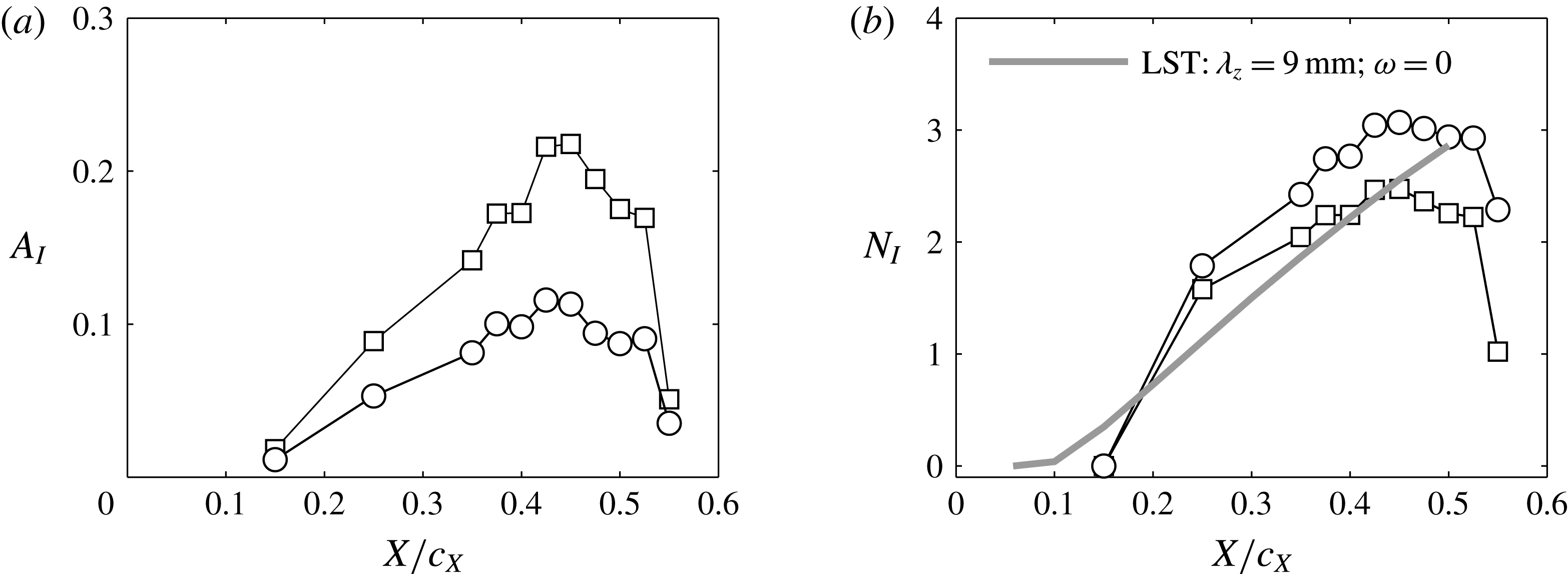
The streamwise growth of the CF mode can be extracted from figure 10(b). There exist several options regarding the specific metric used for the estimation of modal growth. One option is to directly track the maxima, as described by (5.1) (e.g. Haynes & Reed Reference Haynes and Reed2000). A second option is to track the wall-normal integral of the mode shape profiles using (5.2) (e.g. Downs & White Reference Downs and White2013). Although the latter option suffers less from measurement errors and uncertainties, both approaches are followed in this study for comparison with data from previous studies. Results are presented in the form of absolute amplitudes ( $A_{I}$ ) in figure 11(a) and in the form of $N$ -factors ( $N_{I}$ ) in figure 11(b), where the local $N$ -factors are the natural logarithm of the local amplitudes normalised with the amplitude at the first instability point as defined by (5.3). For the experimental results of this study the onset of the primary instability is assumed to occur at the first measured station, $x_{0}=0.15\cdot c_{X}$ . It must be noted here that in order to arrive at the non-dimensional amplitudes using the wall-normal integral metric ( $A_{I}^{int}$ ), the spanwise average boundary layer thickness ( ${\it\delta}_{99}^{z}$ ) is used for non-dimensionalising, as shown in (5.2). This is done following the work of Downs & White (Reference Downs and White2013) and the results presented are in good agreement with the outcomes of their study for similar values of free stream turbulence.

The growth of the primary CF mode is monotonic from the first observation station until approximately $X/c_{X}=0.45$ . Further downstream, a notable reduction of both the local maxima and the integral of the mode shape profile is evident. This indicates primary mode amplitude saturation. Saturation has been typically associated with the rise of nonlinear interactions between the primary mode and secondary instability (Malik et al. Reference Malik, Li, Choudhari and Chang1999; Haynes & Reed Reference Haynes and Reed2000; White & Saric Reference White and Saric2005). Comparison with the LST predictions for the stationary 9 mm mode (presented again in figure 11 b) shows the known limits of the theory, not being able to predict the observed saturation. Despite this, it appears that linear theory can estimate with good agreement the $N$ -factor when the maximum mode shape metric is applied. At the more downstream stations, the forced ${\it\lambda}_{z}^{F}=9$  mm stationary waves start decaying rapidly, with a steep reduction at $X/c_{X}=0.55$ where a fully turbulent boundary layer has developed.

Figure 11.

(a) Non-dimensional amplitudes and (b) $N$ -factors based on the maximum metric ( $A_{I}^{max}$  : ▫) and on the wall-normal integral metric ( $A_{I}^{int}$  : ○) of the mode shape profiles of figure 10(b), computed using (5.1), (5.2) and (5.3). The $N$ -factor curve of the 9 mm stationary mode from LST is shown by the grey solid line. The analysis refers to three full stationary vortices.

Figure 12.

Contours of the velocity standard deviation non-dimensionalised with the time-averaged local external velocity ( $|\bar{V}_{e}^{HWA}|$ ) (10 levels from 0 to 0.1). The contours are stretched along the vertical direction for clarity and presented as seen from upstream.

Additional to the mean flow distortion due to the primary CF mode, the developing boundary layer exhibits an intricate topology of velocity fluctuations. The standard deviation of the velocity fluctuations is computed and non-dimensionalised with the mean local external velocity. Contours of velocity fluctuations are shown in figure 12 for several streamwise stations. Fluctuations observed at $X/c_{X}=0.15$ are mainly associated with the existence of weak travelling CF modes (Deyhle & Bippes Reference Deyhle and Bippes1996). The relatively low free stream turbulence of the wind tunnel facility and the use of discrete roughness elements dictate the dominance of stationary CF instabilities. Nonetheless, the appearance of travelling modes cannot be avoided in an experimental framework (Deyhle & Bippes Reference Deyhle and Bippes1996; Högberg & Henningson Reference Högberg and Henningson1998; Downs & White Reference Downs and White2013).

Further downstream, at stations $X/c_{X}=0.25$ , $X/c_{X}=0.375$ and $X/c_{X}=0.45$ , the spatial topology of velocity fluctuations is strongly influenced by the mean flow distortion due to the primary CF mode (compare with figure 9). The saturation of the primary CF mode downstream of station $X/c_{X}=0.45$ signifies the onset of rapid growth of secondary instability. Similar observations have been established in previous studies (e.g. Högberg & Henningson Reference Högberg and Henningson1998; Kawakami et al. Reference Kawakami, Kohama and Okutsu1999; Malik et al. Reference Malik, Li, Choudhari and Chang1999; Haynes & Reed Reference Haynes and Reed2000; Wassermann & Kloker Reference Wassermann and Kloker2002; White & Saric Reference White and Saric2005). At wing mid-chord, the flow is undergoing turbulent breakdown. The contours of the r.m.s. fields show the rightmost wave experiencing a much higher level of fluctuations. Furthermore, the fluctuation maximum at $z=20$  mm near the wall is indication of the apex of a turbulent wedge (White & Saric Reference White and Saric2005). At the most downstream measured station ( $X/c_{X}=0.55$ ), a fully turbulent boundary layer sets in and redistribution of the fluctuating energy and related dampening of the coherent structures are taking place.

In the region of stationary vortices saturation, the fluctuations are mainly observed in three distinct areas within the spatial domain occupied by a single CF wave (figure 13 a). These areas are associated with unsteady instabilities of a distinct nature (Högberg & Henningson Reference Högberg and Henningson1998; Malik et al. Reference Malik, Li, Choudhari and Chang1999; Wassermann & Kloker Reference Wassermann and Kloker2002; White & Saric Reference White and Saric2005).

One area of high fluctuation intensity can be identified as overlapping the outer side of the upwelling region of the CF vortex. This area is coincident with the local minimum of the spanwise gradient of the mean velocity ( $\partial |\bar{V}^{HWA}|/\partial z$ ) as presented in figure 13(c). Malik et al. (Reference Malik, Li, Choudhari and Chang1999) classified these fluctuations as z-mode secondary instability. These are defined as type-I modes in this paper, following White & Saric (Reference White and Saric2005). A second area of pronounced fluctuating velocity is evident on the top of the CF vortices. Inspecting the velocity shears (figure 13 b) this area overlaps with pronounced wall-normal velocity gradients ( $\partial |\bar{V}^{HWA}|/\partial y$ ). Respectively, this can be identified as the y-mode of the secondary instability (Malik et al. Reference Malik, Li, Choudhari and Chang1999), here defined as type-II mode (Wassermann & Kloker Reference Wassermann and Kloker2002). A third area of strong fluctuations is located at the inner side of the upwelling low momentum air where the $z$ velocity gradients show a local maxima. The disturbances captured in this region are related to the interaction between travelling and stationary primary CF vortices and are named type-III mode (Janke & Balakumar Reference Janke and Balakumar2000; Wassermann & Kloker Reference Wassermann and Kloker2002; Bonfigli & Kloker Reference Bonfigli and Kloker2007). Finally, velocity fluctuations are also evident between the discrete CF vortices in the near-wall region. This area is characterised by the downwelling motion of high momentum flow due to the mean flow distortion induced by the primary CF mode. This results in the formation of a locally thin boundary layer with extremely high wall-normal shear as evident in figure 13(b).

Figure 13.

(a) Contours of velocity standard deviation (10 levels from 0 to 0.1), (b) gradient of time-averaged velocity in the wall-normal direction (10 levels from $-$ 1.7 to 16.6) and (c) in spanwise direction (10 levels from $-$ 3.6 to 2.7). The velocity fields, sampled at $X/c_{X}=0.45$ , are non-dimensionalised with the time-averaged local external velocity ( $|\bar{V}_{e}^{HWA}|$ ) and the lengths with ${\it\lambda}_{z}^{F}$ . The contours are stretched along the vertical direction for clarity and are presented as seen from upstream.

5.3 Comparison between computed and measured boundary layers

As already described in § 4, the LST analysis is based on a laminar boundary layer mean flow, computed numerically using the pressure distribution of figure 2. At this point, a comparison between the computed velocity profiles and the HWA measurements can be performed. In figure 14, this is done for the three most upstream measured stations. The considered HWA profiles are the $z$ -mean of the time-averaged measured planes in order to average the effect of the developing stationary vortices. The computed boundary layer has a prescribed sweep angle of $45^{\circ }$ while the computed velocity components are transformed to match the ones seen by the hot-wire probe.

Figure 14.

Comparison between the computed boundary layer (BL) based on experimental pressure distribution (BL solver) and the hot-wire measurements (averaged along $z$ ), at the most upstream stations. For clarity, only one out of two measured values is reported with a marker symbol.

Figure 15.

Time-averaged velocity magnitude along the stationary crossflow axis measured with tomo-PIV. The local origin at $X_{W}=Z_{W}=0$ coincides with $X/c_{X}=0.45$ and $Z=0$ . The semi-transparent isosurfaces relate to values of $\bar{U}_{W}/\bar{U}_{We}=0.9$ and $\bar{U}_{W}/\bar{U}_{We}=0.8$ . The flow is presented as seen from upstream.

The velocity profiles appear similar for the first stations with a larger discrepancy at station $X/c_{X}=0.35$ where the measured velocity field is evidently distorted by the stationary CF vortices (see also figure 10 a). Instead, the satisfactory agreement at $X/c_{X}=0.15$ indicates that the curvature of the model, not modelled in the boundary layer solver, is not very relevant at this station. This comparison further corroborates the estimations of the LST for the most upstream regions of the studied flow.

5.4 Tomographic PIV measurements

The analysis of the primary boundary layer instability is further expanded to the results of the tomo-PIV experiment. As mentioned in § 3, the measured velocity field is aligned with the coordinate system of the primary stationary vortices $(X_{W}Y_{W}Z_{W}\equiv X_{W}y_{t}Z_{W})$ . The time-averaged flow field of the velocity component along the stationary vortices axes, non-dimensionalised with the time-averaged external velocity, is presented in figure 15. Three $y_{t}$ – $Z_{W}$ planes, at the $X_{W}$ locations corresponding to the most upstream end, to the most downstream end and to the centre of the measured domain, are shown with 10 contour levels. Additionally, two isosurfaces pertaining to levels of velocity of $\bar{U}_{W}/\bar{U}_{We}=0.9$ and $\bar{U}_{W}/\bar{U}_{We}=0.8$ are also plotted to facilitate the visualisation of the three-dimensional evolution of the vortical structures. The point at $X_{W}=0$ is at $X/c_{X}=0.45$ while the $Z_{W}=0$ is at $Z=0$ (wing mid-span). The position of the wall is linearly extrapolated from the measured velocity profiles. Almost five stationary waves are captured by this measurement. Their spacing is relatively constant, corresponding approximately to a wavelength along $Z_{W}$ of 6.9 mm. A wavelength of 6.9 mm in the $X_{W}Y_{W}Z_{W}$ coordinate system corresponds to 9 mm in the $xyz$ domain, consistent with the spacing of the discrete roughness elements at the leading edge. A small discrepancy is observed regarding the position of the rightmost wave at approximately $Z_{W}=17$  mm. This could be attributed to non-uniformities of the discrete roughness elements or to occasional debris depositing on the model surface, slightly displacing this vortex.

The unprecedented application of tomo-PIV for the measurement of transitional swept wing boundary layers necessitates the rigorous comparison of the measurements against established techniques such as HWA. This requires some care given the different reference systems and velocity components measured by the two techniques. Towards this goal, a plane aligned with $y_{t}$ – $z$ is extracted at $X/c_{X}=0.45$ from the volume presented in figure 15, thus coinciding with the hot-wire measured plane. The velocity components are then transformed such to match the signal measured by the hot-wire ( $|V^{HWA}|=(U^{2}+V^{2})^{1/2}$ ). The result of such comparison is presented in figure 16 for the time-averaged velocity. The values of the velocities are non-dimensionalised with the time-averaged local external velocity while the wall position is linearly extrapolated from the measured data. The agreement between the two measurement techniques is striking.

At the upper-left corner of the two contours three ( $+$ ) symbols are plotted to show the spatial $y_{t}$ - $z$ resolution of the two experiments. (Note that the contours are stretched along the $y_{t}$ direction.) In spite of the higher wall-normal resolution of the hot-wire measurements compared to tomo-PIV, the latter appears to be capturing the strong shears due to the modulated flow with the same accuracy. A further comparison of the two velocity fields is presented in terms of velocity profiles in figure 16(c). The velocity distribution across the wall-normal direction, at the two spanwise stations denoted with the same markers on figure 16(a) and 16(b) and pertaining respectively to regions of reduced and strong wall-normal shears, is measured by the two techniques with good agreement, showing a maximum discrepancy of $0.058|\bar{V_{e}}^{HWA}|$ .

Figure 16.

Contours of time-averaged velocity magnitude, non-dimensionalised with the mean local external velocity (10 levels from 0 to $|\bar{V}_{e}^{HWA}|$ ) from (a) HWA and (b) tomo-PIV. The spatial resolution along $z$ and $y_{t}$ of the two measurements is presented with the ( $+$ ) symbols at the upper-left corner of the contours (note that the contours are stretched along the $y_{t}$ direction). (c) Velocity profiles at the stations indicated with identical symbols on contours (a) and (b). For clarity only one out of four measured values is reported with a marker symbol.

It now becomes important to further establish a comparison between the two experiments in measuring the statistical quantities of the unsteady field. This comparison is presented in figure 17 where the r.m.s. of the velocity fluctuations, non-dimensionalised with the external velocity, is shown. A notable feature of the fluctuation field captured by tomo-PIV is the elevated level measured in the free stream. This effect is attributed to the inherent limits associated with PIV in general and tomo-PIV specifically. The background r.m.s. level has an average value of $0.015\bar{V}_{e}^{HWA}$ that corresponds to the error estimated in § 3.6.

Despite the elevated fluctuation levels in the free stream, the tomo-PIV measurement captures the local maxima associated with type-I, type-II and type-III instabilities in both magnitude and location. Both inner and outer upwelling regions, as well as the top region, are in relative agreement to the hot-wire measurements. Unfortunately, the same cannot be said for the near-wall portion of the downwelling region (centred at $z\approx 0,9,18$  mm in figure 17). At this region, the inherent downwelling action of the primary CF instability results in elevated shear near the wall, as showed in figure 13(b). Such high shears are beyond the measurable threshold of $0.5~\text{px}~\text{px}^{-1}$ reported by Scarano (Reference Scarano2002) for PIV measurements. It is believed that the pronounced errors are not deemed disruptive to the conclusions of this study because they appear in a region not associated with a particular instability mode. For the remainder of the analysis of the unsteady flow features, the near-wall region of the tomo-PIV fields ( $y_{t}<0.95$  mm indicated with the dotted line on the contour) will not be taken into account. The r.m.s. maximum of the inner upwelling region, pertaining to the type-III mode, appears also partially affected by the described measurement error. This is again disregarded to be influencing the analysis of § 6.3 as POD allows the identification of spatially coherent structures, thus filtering out most of the measurement noise (Raiola, Discetti & Ianiro Reference Raiola, Discetti and Ianiro2015).

Figure 17.

Contours of the velocity standard deviation, non-dimensionalised with the mean local external velocity (12 levels from 0 to $0.12|\bar{V}_{e}^{HWA}|$ ) from (a) HWA and (b) tomo-PIV. The black dotted line at $y_{t}=0.95$  mm in the tomo-PIV contour indicates the region disregarded in the unsteady flow analysis of § 6.3.

A slice at $X/c_{X}=0.45$ of the volume shown in figure 15 is presented in figure 18 for all the three velocity components. Additionally, the velocity components are presented in the primary CF vortices coordinate system ( $U_{W}V_{W}W_{W}$ ). The $\bar{U}_{W}$ component dominates over the two in-plane components ( $\bar{V_{W}}$ and $\bar{W_{W}}$ ) by two orders of magnitude. The relative magnitude of the three velocity components reveals the effectiveness of the in-plane components in modifying the mean boundary layer and thus the out-of-plane velocity. The wall-normal velocity maxima at $z=5.0$  mm and 14.0 mm are responsible for the upwelling of the low momentum flow from the lower regions of the boundary layer. The minimum at $z=9$  mm is instead the effect of the downwelling motion with the consequent transport of higher momentum flow from the boundary layer outer edge towards the wing surface. At $z=2.8$  mm and $z=11.8$  mm a second local minimum of the wall-normal velocity is observed. This is located in a region where Malik et al. (Reference Malik, Li and Chang1994), Wassermann & Kloker (Reference Wassermann and Kloker2002) and Bonfigli & Kloker (Reference Bonfigli and Kloker2007) reported a second stationary vortex, the effect of which was found to be not relevant in the transition scenario. The spanwise velocity ( $\bar{W_{W}}$ ) contour reveals the crossflow velocity in the regions near the wall. The non-zero value of $\bar{W_{W}}$ at the outer edge is instead dictated by the chosen coordinate system. As the stationary CF axis is not exactly aligned with the inviscid flow, what is plotted contains the projection of the streamwise velocity along the $Z_{W}$ direction.

Summarising, although the primary waves are manifested as relatively weak spanwise perturbations of the $V_{W}$ and $W_{W}$ components, the change they induce in the axial velocity component is dramatically larger. Although this is a known feature of CF instability, the simultaneous characterisation of all three components of velocity was so far possible only in the realm of numerical simulations (Wassermann & Kloker Reference Wassermann and Kloker2002; Bonfigli & Kloker Reference Bonfigli and Kloker2007). The experimental measurement of such features indicates the merits of tomo-PIV as a diagnostic tool for this type of flow.

Figure 18.

Non-dimensional time-averaged velocity components sampled along a constant chordwise plane at $X/c_{X}=0.45$ . (a) $\bar{U}_{W}/\bar{U}_{We}$ (10 levels, from 0 to 1) and vectors of $(\bar{V}_{W}^{2}+\bar{W}_{W}^{2})^{1/2}/\bar{U}_{We}$ (reference vector at the upper-left corner). For clarity, only one in three vectors is plotted along $z$ . (b) $\bar{V}_{W}/\bar{U}_{We}$ , $\bar{W}_{W}/\bar{U}_{We}$ .

6.1 Spectral characteristics

As discussed in the previous section, the fluctuation field features three local maxima, corresponding to the location of the velocity gradients (see figure 13). At these locations, the time series of the velocity fluctuations were used to compute the power spectral density ( ${\it\Phi}_{V^{\prime }}$ ) using the average periodogram method introduced by Welch (Reference Welch1967). A single-point HWA measurement consists of $2\times 10^{5}$ instantaneous readings. The spectra were computed for segments of 5000 samples, with a relative overlap of 50 %, averaged together. All the presented spectra feature a frequency resolution of ${\it\delta}_{f}=10$  Hz.

Figure 19.

Non-dimensional spectra of the velocity fluctuations, for six chordwise stations, at the locations indicated by the (○) markers in the inset figure (coded with the corresponding colours). Inset: contour of the time-averaged velocity field (black lines, 10 levels from 0 to 1) and velocity fluctuations field (grey scale, 10 levels from 0 to 0.084) non-dimensionalised with the mean local external velocity $|\bar{V}_{e}^{HWA}|$ , at $X/c_{X}=0.475$ .

The non-dimensional spectra ( $({\it\Phi}_{V^{\prime }}\cdot {\it\delta}_{f}/U_{\infty }^{2})^{1/2}$ ) are plotted in figure 19 for several chordwise stations. The lines are coded with the same colours of the bullet markers of the contour, presented in the inset, where the velocity signals are sampled. The analysis of the three fluctuation regions shows respective dominance of significantly disparate spectral content and diverse streamwise evolution. At the first considered station, $X/c_{X}=0.375$ (first panel of figure 19), the inner upwelling region (marked by the light grey colour as in the inset) is characterised by pronounced spectral energy in a band of low Strouhal numbers between $St=15$ ( $f=300$  Hz) and $St=25$ ( $f=550$  Hz). At higher frequencies, the spectral energy significantly drops to the level of background noise. Several narrow spikes appear above $St=250$ which can be attributed to electronic noise. Additionally, a low power frequency band from $St=150$ and $St=500$ is present which is traced to inherent characteristics of the hot-wire bridge and does not correspond to physical events (Saddoughi & Veeravalli Reference Saddoughi and Veeravalli1996). The low frequencies dominating the inner upwelling region are consistent with observations of Deyhle & Bippes (Reference Deyhle and Bippes1996), Malik et al. (Reference Malik, Li, Choudhari and Chang1999) and White & Saric (Reference White and Saric2005) and are attributed to primary travelling crossflow instabilities which initially develop in the boundary layer independently of the primary standing modes. Later, when the stationary vortices reach a considerable amplitude, these travelling waves undergo the spanwise modulation imposed on the boundary layer by the steady modes (Fischer & Dallmann Reference Fischer and Dallmann1991; Högberg & Henningson Reference Högberg and Henningson1998; Janke & Balakumar Reference Janke and Balakumar2000; Bonfigli & Kloker Reference Bonfigli and Kloker2007). This is further confirmed by the predictions of LST which identified amplified modes around $St=15$ ( $f=300$  Hz) (figure 7 a).

The fluctuations in the outer region of the upwelling flow (indicated with the black colour) are instead characterised by a pronounced band of Strouhal numbers between $St=124$ ( $f=2.5$  kHz) and $St=348$ ( $f=7$  kHz). Such high frequencies have been typically associated with secondary instability of the Kelvin–Helmholtz type (Bonfigli & Kloker Reference Bonfigli and Kloker2007) arising as a nonlinear perturbation of the primary stationary CF mode (cf. Malik et al. Reference Malik, Li, Choudhari and Chang1999; Janke & Balakumar Reference Janke and Balakumar2000; White & Saric Reference White and Saric2005).

Moving downstream, the energy content of the associated frequency bands is drastically increased indicating growth of all unsteady modes. The spectra at $X/c_{X}=0.425$ show that both the low-frequency band associated with the inner side of the upwelling region of the CF vortex and the high-frequency hump occurring in the outer side, exhibit large amplitude growth. Moreover the spectrum of fluctuations in the top region of the primary wave (marked in dark grey), coinciding with a maximum of the velocity gradient along $y_{t}$ (see figure 13 b), shows also a band of high energy centred at $St=373$ ( $f=7.5$  kHz). This indicates destabilisation of the type-II mode as well (Malik et al. Reference Malik, Li, Choudhari and Chang1999; White & Saric Reference White and Saric2005).

At $X/c_{X}=0.45$ the type-III mode (light grey line), sampled in the inner side of the upwelling region, further amplifies. Additionally, the two higher harmonics of this mode (at approximately $St=46$ ( $f=925$  Hz) and $St=65$ ( $f=1300$  Hz)) become evident at this station. At this station, the type-I high-frequency mode greatly enhances its magnitude compared to the previous chord station. It features a larger growth than that experienced by the low-frequency travelling waves, suggesting a stronger growth rate for this secondary instability (cf. Högberg & Henningson Reference Högberg and Henningson1998). Sudden growth occurs as well to the higher-frequency type-II mode (dark grey line) sampled in the top region of the primary vortex, reaching a comparable amplitude to the type-I mode just discussed.

Further downstream, at $X/c_{X}=0.475$ , the low-frequency fluctuations in the vortex inner upwelling region and those in the top region are further enhanced, although the magnitude of the background neighbouring frequencies is also increased. The type-II mode on the upper region of the primary vortex shows a steep increase, overcoming, at this location, the magnitude of the type-I instability. The last two stations, where the spectral analysis is performed, are located at $X/c_{X}=0.50$ and $X/c_{X}=0.525$ . The two high-frequency type-I and type-II modes appear to peak in energy but they also appear to be almost overtaken by the broadband fluctuations pertaining to a more turbulent boundary layer. The low-frequency mode instead does not show any appreciable change between $X/c_{X}=0.45$ and $X/c_{X}=0.525$ . This further suggests the independence of the type-III mode from the growth of secondary instability although the growth of all three modes appears to be related to the saturation of the stationary vortices, as will be described later.

6.2 Streamwise evolution

The analysis of the spectra presented so far pertains to rigorous amplification of the three unsteady modes in the region between primary mode amplitude saturation ( $X/c_{X}\approx 0.45$ ) and turbulent onset ( $X/c_{X}\approx 0.50$ ). A way to track this evolution is presented by White & Saric (Reference White and Saric2005) and Downs & White (Reference Downs and White2013) and consists of computing the growth rates of the unsteady modes. To do this, the velocity fields are bandpass filtered, by means of zero phase shift fourth-order digital filtering, in the respective frequency bands. Root-mean-square contours of the bandpass filtered fields are presented in figure 20 for stations $X/c_{X}=0.45$ , $X/c_{X}=0.475$ and $X/c_{X}=0.50$ . Additionally the time-averaged velocity field respective to the station is superimposed. The contours on the first column on the left and indicated with band 1, refer to the band $17.4\leqslant St\leqslant 27.3$ ( $350~\text{Hz}\leqslant f\leqslant 550~\text{Hz}$ ) pertaining to the type-III instability (not to be confused with the type-I mode). Contours indicated with band 2 correspond to the range $248.0\leqslant St\leqslant 298$ ( $5~\text{kHz}\leqslant f\leqslant 6~\text{kHz}$ ) related to the type-I mode. Band 3 relates to the range $348\leqslant St\leqslant 397$ ( $7~\text{kHz}\leqslant f\leqslant 8~\text{kHz}$ ), pertaining to the type-II mode. The contours are non-dimensionalised with the free stream velocity ( $U_{\infty }$ ). Note that the band 1 contours attain larger values than the ones of bands 2 and 3.

Figure 20.

Bandpass filtered velocity fluctuation fields (grey scale) and time-averaged velocity fields (black lines, 10 levels from 0 to $U_{\infty }$ ). Frequency band 1: $17.4\leqslant St\leqslant 27.3$ ( $350~\text{Hz}\leqslant f\leqslant 550~\text{Hz}$ ) (10 levels from 0 to $0.24U_{\infty }$ ), band 2: $248.0\leqslant St\leqslant 298.3$ ( $5~\text{kHz}\leqslant f\leqslant 6~\text{kHz}$ ) (10 levels from 0 to $0.6U_{\infty }$ ) and band 3: $348.0\leqslant St\leqslant 397.8$ ( $7~\text{kHz}\leqslant f\leqslant 8~\text{kHz}$ ) (10 levels from 0 to $0.6U_{\infty }$ ).

It becomes evident that the three modes possess characteristic topological arrangement and streamwise development. The spatial locations, with respect to the primary vortices, pertaining to the three modes are revealed, confirming previous observations by e.g. Högberg & Henningson (Reference Högberg and Henningson1998), Malik et al. (Reference Malik, Li, Choudhari and Chang1999) and White & Saric (Reference White and Saric2005). Moving past the wing trailing edge, it can be seen how the high-frequency modes grow strongly passing from $X/c_{X}=0.45$ to $X/c_{X}=0.50$ . The low-frequency mode, although having a larger amplitude, does not show such a steep growth, as already commented.

Although the absolute magnitude of r.m.s. intensity reveals the overall growth of each mode, a more robust evaluation of the growth rates is sought. To this end the disturbances amplitude expressed by (6.1) (as defined by White & Saric (Reference White and Saric2005) and Downs & White (Reference Downs and White2013)) is introduced, pertaining to a spatial average, along $z$ and $y_{t}$ , of the r.m.s. of the bandpass filtered velocity fluctuations. Here $t_{rms}\{|V_{BP}^{HWA}|/|\bar{V}_{e}^{HWA}|\}$ represents the r.m.s. of the time series of the non-dimensional bandpass filtered velocity field, ${\it\delta}_{99}^{z}$ is again the spanwise-averaged boundary layer thickness and $z_{max}$ denotes the spanwise integration length chosen to accommodate three primary crossflow waves ( $z_{max}=3{\it\lambda}_{z}^{F}=27$  mm)

Using the computed amplitudes, $N$ -factors of the unsteady modes can be estimated based on the reference amplitude at $x_{0}=0.35c_{X}$

The computed amplitudes ( $A_{II}$ ) are presented in figure 21(a), while the $N$ -factors ( $N_{II}$ ) of the unsteady modes are shown in figure 21(b). The need to present both the curves resides in the observation that the choice of the initial normalising amplitudes for the different modes is not trivial and can lead to misleading conclusions. The low-frequency mode exhibits the strongest and earliest growth. Indeed, within only 20 % of the chord, spanning from $X/c_{X}=0.35$ to $X/c_{X}=0.55$ , the amplitude of fluctuations attributed to the low-frequency mode increases by approximately two orders of magnitude. Moreover, it can be seen that this mode grows monotonically in the considered range, with a steeper slope between $X/c_{X}=0.45$ and $X/c_{X}=0.475$ .

It is important to note here that since travelling crossflow modes essentially sweep the measurement plane, their fluctuation intensity would be expected not to significantly vary in the $z$ direction. It is evident from figure 20(a) that this is not the case as the low-frequency band is only dominant in the inner upwelling region of the standing CF vortex. As discussed, this is caused by the interaction with the stationary CF vortices. Moreover, since this is a primary instability mechanism (Fischer & Dallmann Reference Fischer and Dallmann1991; Högberg & Henningson Reference Högberg and Henningson1998; Janke & Balakumar Reference Janke and Balakumar2000; Bonfigli & Kloker Reference Bonfigli and Kloker2007), its growth along the streamwise direction is expected to not show the explosive nature of the secondary modes. After the saturation of the steady modes however, the amplitude of this mode shows larger values. The two high-frequency modes instead show the previously reported (Wassermann & Kloker Reference Wassermann and Kloker2002; White & Saric Reference White and Saric2005) sudden growth from $X/c_{X}=0.45$ and, within only the 10 % of the wing chord, they amplify to 30 (type-I) and 20 (type-II) times their initial amplitude.

It can also be seen that the three inspected frequency bands drive the amplitude of the full-spectrum fluctuations, which also shows a sudden enhancement after station $X/c_{X}=0.45$ . At the last considered station $X/c_{X}=0.55$ , turbulent breakdown occurs, as seen in figure 9 and is further indicated by the steeper slope of all the curves. The three bands show comparable amplitudes, reaching approximately 60 % of the total fluctuation amplitude. At this station, the bands cannot be related any more to the instability modes.

Figure 21.

(a) Amplitudes and (b) $N$ -factors of total and bandpass filtered velocity fluctuations, computed using (6.1) and (6.2). Same frequency bands as figure 20. This analysis refers to the flow field pertaining to three full stationary vortices.

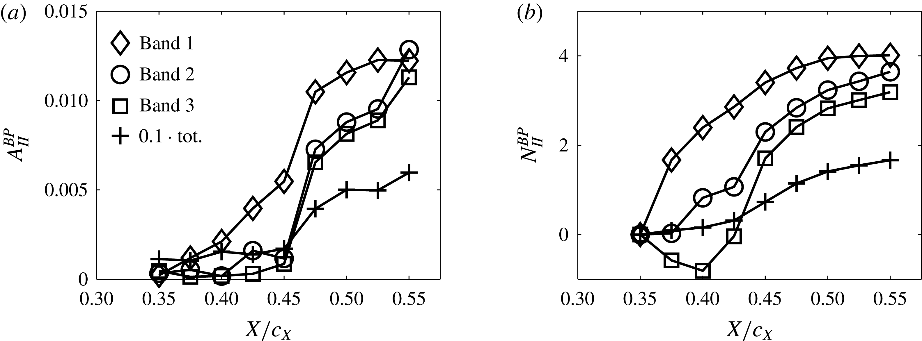
6.3 Spatial organisation

The large disparity of length scales and time scales associated with the instability modes in a swept wing boundary layer necessitate the deployment of robust and objective mode identification techniques. One such technique is POD, originally introduced by Lumley (Reference Lumley, Yaglom and Tatarsky1967) for identification of coherent turbulent structures. This is a powerful technique which capitalises on the spatial coherence of orthogonal modes in order to identify and prioritise them with respect to their energy content.

In this experiment, POD was applied on the full set of 500 instantaneous tomo-PIV flow fields using the snapshot technique introduced by Sirovich (Reference Sirovich1987). Furthermore, the investigated volume was cropped compared to the full tomo-PIV domain of figure 15. This was done for several reasons: firstly, POD inherently identifies spatially coherent unsteady modes within a given flow field. In the case of CF instability-dominated boundary layers, these would effectively be the primary travelling waves and secondary instability vortices. Additionally, these modes exhibit strong nonlinear behaviour with respect to the standing CF mode (see § 6.2 and work of Malik et al. (Reference Malik, Li and Chang1994)) but not with the high-frequency instabilities developing on a neighbouring stationary CF vortex, as reported by Bonfigli & Kloker (Reference Bonfigli and Kloker2007). These observations bring specific considerations regarding the application of POD to a flow field encompassing multiple standing CF vortices. The instability modes developing within each standing CF vortex will be directly associated with the strength and topology of their respective carrier CF wave. Although, the primary waves have been forced with identical roughness elements, total similarity cannot be guaranteed in an experimental framework. Any slight disparity between individual standing CF vortices and in their secondary destabilisation would consequently introduce discrepancies between sets of unsteady modes in terms of amplitude and spatial coherence which would degrade the ability of POD to identify them. Based on this, a domain encompassing a single standing CF vortex was selected for POD analysis by cropping the full tomo-PIV volume in the spanwise range of $0~\text{mm}\leqslant z\leqslant 6~\text{mm}$ . A second consideration is the apparent failure of tomo-PIV to capture the near-wall region, as evident by the discrepancies in figure 17. As discussed, this is due to inherent limits of PIV in regions of high shear. Fortunately, the bandpass filtered fluctuation distributions presented in figure 20 indicate little modal content in the near-wall region, other than a fraction of the type-III mode. Following this, the considered domain for POD was further cropped to dismiss the near wall-region ( $y_{t}<0.95$  mm).

Figure 22.

Relative turbulent kinetic energy distribution of the first 20 POD modes.

The relative turbulent kinetic energy distribution (TKE) of the first twenty POD modes is shown in figure 22. The first POD mode clearly dominates in the unsteady flow field with approximately 16 % of the total fluctuation kinetic energy. The energy content of the following modes diminishes rapidly. At this point, some notes are necessary regarding the interpretation of POD modes. In typical application cases such as bluff body aerodynamics (Nati et al. Reference Nati, Kotsonis, Ghaemi and Scarano2013) or turbulent breakdown of free jets (Violato & Scarano Reference Violato and Scarano2013), the inherent ability of POD to prioritise spatially coherent modes according to their energy content is rather straightforward. In contrast, in highly multiscale, nonlinear problems such as transitional boundary layers, POD modal energy is weakly coupled to the importance of the respective mode in the transition process. In the present study, spatially coherent modes corresponding to the developing instabilities within the standing CF vortex are sought. It is already known from the existing hot-wire measurements (cf. § 6.2) and previous investigations (Wassermann & Kloker Reference Wassermann and Kloker2002) that these modes are rather weak compared to the free stream velocity, and hence prone to be overshadowed by other sources such as measurement noise. Finally, it must be stressed that the exact sorting of these modes is additionally dependent on the domain of the flow field considered for POD.

Considering the previous points, it becomes important to identify the modes relevant to the transition process based on features other than their energy content. One such feature is the expected spatial wavelength associated with the mode, which can be derived using the Taylor hypothesis from the previously described hot-wire measurements. A second feature stems from the fact that the sought instability modes are inherently convective (Kawakami et al. Reference Kawakami, Kohama and Okutsu1999; Wassermann & Kloker Reference Wassermann and Kloker2002; Bonfigli & Kloker Reference Bonfigli and Kloker2007). As such, the POD procedure will generate a harmonically coupled pair of POD modes, shifted by ${\rm\pi}/2$ , for each physical convecting coherent structure (Van Oudheusden et al. Reference Van Oudheusden, Scarano, Van Hinsberg and Watt2005). Both these features have been used as selection criteria in this study in order to identify the POD modes corresponding to the relevant instability modes in the transitional boundary layer. Following this approach, four modes ( ${\it\Phi}_{6}$ , ${\it\Phi}_{7}$ , ${\it\Phi}_{9}$ and ${\it\Phi}_{10}$ ) have been selected and are presented in §§ 6.3.2 and 6.3.3. Before moving to the analysis of the secondary instability modes, the first POD mode ( ${\it\Phi}_{1}$ ) is inspected due to its considerably high energy content and particular spatial topology (§ 6.3.1).

Figure 23.

Isosurfaces of $U_{W}/\bar{U}_{We}=\pm 0.086$ of POD mode ${\it\Phi}_{1}$ . Three contours of $\bar{U}_{W}/\bar{U}_{We}$ at $X_{W}-15,0$ and 15 mm (10 levels from 0 to 1).