



1. Introduction
Large-scale coastal morphology is a consequence of the sediment transport fields and associated erosion and deposition. In the classical application of morphological models, without the presence of vegetation, the long-term migration of the coastline is typically associated with the long-shore sediment transport, while short-term coastline oscillations are associated with the cross-shore sediment transport (Fredsøe & Deigaard Reference Fredsøe and Deigaard1992; Komar Reference Komar1998). In both cases, the layman's description is that processes in the wave boundary layer stir up the sediment, while a mean current advects the sediment. This understanding of sediment stirring and advection mechanisms has been condensed into engineering models for large-scale morphological models (Lesser et al. Reference Lesser, Roelvink, van Kester and Stelling2004; van Rijn Reference van Rijn2007; van der A et al. Reference van der A, Ribberink, van der Werf, O'Donoghue, Buijsrogge and Kranenburg2013).
The practical engineering models have their applicability limited to sandy coastal environments (with and without bedforms), so their applicability for vegetated habitats is questionable irrespective of the considerable academic and practical engineering interest in computing their short- and long-term morphodynamic processes (The World Bank 2017; Bridges et al. Reference Bridges, Bourne, King, Kuzmitski, Moynihan and Sudel2018; EcoShape 2020; Morris et al. Reference Morris2021). Efforts with large-scale pilot studies, field and laboratory experiments have provided valuable information, but there are still several outstanding questions that need to be researched before practical engineering models describing morphodynamics in vegetated habitats reach the same maturity as those for unvegetated regions.
The advective mean flow field in vegetated habitats is qualitatively different from unvegetated regions, where the latter consists of a strong undertow within the surf zone with and without breaker bars (Dyhr-Nielsen & Sørensen Reference Dyhr-Nielsen and Sørensen1970; Deigaard & Fredsøe Reference Deigaard and Fredsøe1989; Ting & Kirby Reference Ting and Kirby1994; Jacobsen & Fredsøe Reference Jacobsen and Fredsøe2014; Fernandez-Mora et al. Reference Fernandez-Mora, Ribberink, Van der Zanden, Van der Werf and Jacobsen2016; Van der Zanden et al. Reference Van der Zanden, Van der A, Hurther, Cáceres, O'Donoghue and Ribberink2017). The main differences arising from a canopy are (i) weak in-canopy mean velocities, (ii) a strong mean streaming velocity on top of the canopy, positive in the wave propagation direction and (iii) a return flow between the top of the canopy and the still water level (Luhar et al. Reference Luhar, Coutu, Infantes, Fox and Nepf2010; Abdolahpour, Hambleton & Ghisalberti Reference Abdolahpour, Hambleton and Ghisalberti2017), which means that strong advection of sediment near the bed by an undertow, as known from sandy beaches, is suppressed by the vegetation, and this impacts the mean sediment transport patterns. On the other hand, it has recently been documented that the in-canopy turbulence results in earlier initiation of sediment transport than for an unvegetated seabed (Tinoco & Coco Reference Tinoco and Coco2014, Reference Tinoco and Coco2018).
Finally, focusing on the bottom boundary layer dynamics, the literature has a wealth of documentation on the oscillatory and wave boundary layers where friction factors, laminar-to-turbulent transition and hydraulically smooth and rough conditions are extensively studied (Bagnold Reference Bagnold1946; Grant & Madsen Reference Grant and Madsen1979; Sleath Reference Sleath1987; Jensen, Sumer & Fredsøe Reference Jensen, Sumer and Fredsøe1989; van der A, Scandura & O'Donoghue Reference van der A, Scandura and O'Donoghue2018; Dunbar et al. Reference Dunbar, Van der A, O'Donoghue and Scandura2023a,Reference Dunbar, Van der A, Scandura and O'Donoghueb). Furthermore, the mean streaming processes due to finite wavelengths and nonlinear oscillatory free stream conditions are also well understood over a horizontal seabed (Longuet-Higgins Reference Longuet-Higgins1957; Trowbridge & Madsen Reference Trowbridge and Madsen1984; Brøker Reference Brøker1985). The works, however, are limited to flat surfaces with possibly a shallow layer of protruding roughness elements (rocks and ripples). On the other hand, the author has found no works related to the oscillatory bottom boundary layer in the presence of vertically protruding vegetation stems and how these affect friction factors, boundary layer thickness, phase leads and mean wave-induced flow due to either finite wavelengths or nonlinear free-stream velocities.
Neshamar et al. (Reference Neshamar, Jacobsen, Van der A and O'Donoghue2023) presented a description of the in-canopy bulk oscillatory velocity and showed that the phase lead of the in-canopy bulk velocity over the free stream velocity is significant. They applied a two-layer model approach to evaluate the bulk in-canopy velocity and free-stream velocity, where the former is defined as the average over the height of the stems. Given the averaging over the stems, their model captures neither details of the bottom boundary layer and shear layer dimensions nor the associated friction factors. Knowing that the bottom shear stress typically leads over the near-bed velocity above the boundary layer (Jensen et al. Reference Jensen, Sumer and Fredsøe1989; Fredsøe et al. Reference Fredsøe, Sumer, Kozakiewicz, Chua and Deigaard2003) suggests that a significant phase lead of the bottom shear stress to the free-stream velocity shall be expected by the introduction of vegetation. This increase in phase lead will subsequently affect sediment transport and its ability to escape from the canopy through vertical diffusion. Regarding the bottom boundary layer, Jacobsen, Van Gent & Fredsøe (Reference Jacobsen, Van Gent and Fredsøe2017, their Appendix A) made the qualitative observation that oscillatory boundary layers of constant viscosity – for the same near-bed velocity – are thinner within a filter layer of crushed rocks compared with a case without the filter layer. The case without a porous layer on top of the seabed will be referred to as the unvegetated boundary layer throughout. The qualitative observation by Jacobsen et al. (Reference Jacobsen, Van Gent and Fredsøe2017) effectively means that the friction factor based on the near-bed velocity will be larger in a crushed rock layer or any other drag-dominated structure such as vegetation stems, ultimately meaning that present-day friction factor diagrams are not applicable for the determination of loading on the sedimentary seabed.
The present work offers a theoretical description of vegetated oscillatory boundary layers based on (i) a linearised analytical solution akin to the Stokes oscillatory wave boundary layer and (ii) a turbulent one-dimensional numerical solution periodic in time. The work extends the solution to the nonlinear, oscillatory bulk in-canopy flow by Neshamar et al. (Reference Neshamar, Jacobsen, Van der A and O'Donoghue2023) from their two-layer model approach to a vertically resolved solution including viscous effects in the bottom boundary layer and in the shear layer on top of the canopy. This allows for the presentation of novel results with respect to friction factors within canopies (and their deviation from the unvegetated counterparts), boundary and shear layer thicknesses and the phase lags between shear stresses and the in-canopy bulk velocity. The mathematical models and their verification are presented in § 2. Subsequently, the bottom boundary layer characteristics such as friction factors, boundary layer thickness and phase leads over the free-stream velocity are investigated (§§ 3.1 and 3.2). The mean velocity profile due to finite wavelength effects (§ 3.3) and nonlinear free stream velocities (§ 3.4) are also investigated. The work is concluded with a discussion and conclusions.
2. Mathematical model
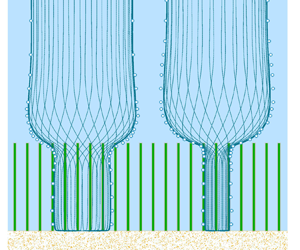
The mathematical model describes the viscous oscillatory flow in the presence of rigid stems (see figure 1). The treatment as oscillatory means that  $\partial \phi /\partial x =\partial \phi /\partial y = 0$ on any quantity
 $\phi$ within and above the canopy (
 $x$ and
 $y$ are horizontal Cartesian coordinates) when
 $\phi$ is averaged over a sufficiently large horizontal area. Here, ‘sufficiently large’ refers to several stem spacings along both
 $x$ and
 $y$ in order to absorb local stem processes (flow amplification, vortex shedding, etc.) in the averaged
 $\phi$; however, it is not necessary to average over larger areas scaled by, for instance, the wavelength since the external forcing is purely oscillatory. The oscillatory flow in and above a canopy is then described by the following dimensional form of the horizontal momentum equation (Neshamar et al. Reference Neshamar, Jacobsen, Van der A and O'Donoghue2023, combination of their equations (2)–(4)):
 \begin{equation} \Bigg(1+C_m\hat{N}\frac{\hat{d}^2{\rm \pi}}{4}\Bigg)\frac{\partial }{\partial \hat{t}}\frac{\hat{u}}{n} = \frac{\partial \hat{u}_0}{\partial \hat{t}} + \frac{1}{n}\frac{\partial}{\partial \hat{z}} \left[\left(\hat{\nu} +\hat{\nu}_t\right)\frac{\partial \hat{u}}{\partial \hat{z}}\right] - \frac{1}{2}C_Dn^{-2}\hat{d}\hat{N}|\hat{u}|\hat{u}. \end{equation}
Here,  $\hat {u}(\hat {z},\hat {t})$ is the dimensional horizontal filter velocity,
 $\hat {u}_0(\hat {t})$ is the dimensional free-stream velocity (far above the canopy),
 $\hat {t}$ is the dimensional time,
 $\hat {\nu }$ is the dimensional kinematic molecular viscosity,
 $\hat {\nu }_t$ is the dimensional turbulent eddy viscosity and
 $\hat {z}$ is the dimensional vertical coordinate. Further,
 $n = 1 - \hat {N}\hat {d}^2{\rm \pi} /4$ is the porosity of the canopy,
 $\hat {N}$ is the number of stems per unit area,
 $\hat {d}$ is the diameter of the circular stems,
 $C_m$ is the inertia coefficient and
 $C_D$ is the drag coefficient.
Sketch of the oscillatory flow in a rigid canopy. Present viscous model is shown in blue, while the two-layer model by Neshamar et al. (Reference Neshamar, Jacobsen, Van der A and O'Donoghue2023) is shown dashed red for comparison. (a) Model domain including shear layer on top of the canopy. (b) Indication of the ‘infinite’ vegetation scenario with the oscillatory bottom boundary layer.

The dimensional quantities (marked by  $\hat{\ }$ ) are made non-dimensional by the first harmonic velocity amplitude,
 $\hat {u}_{1}$, and the cyclic frequency for the first harmonic,
 $\hat {\sigma}_1 = 2{\rm \pi} /\hat {T}$;
 $\hat {T}$ is the regular wave period:
 $u = \hat {u}/\hat {u}_1$,
 $z = \hat {z}/\hat {a}_1=\hat {\sigma }_1\hat {z}/\hat {u}_1$,
 $t=\hat {t}\hat {\sigma }_1$ and
 $\hat {a}_1=\hat {u}_1/\hat {\sigma }_1$ is the wave orbital amplitude. The non-dimensional momentum equation then reads
 \begin{equation} \varGamma_I\frac{\partial u}{\partial t} = \frac{\partial u_0}{\partial t} + \frac{\partial}{\partial z}\left[\frac{1}{Re_n}\left(1 + \frac{\hat{\nu}_t}{\hat{\nu}}\right)\right]\frac{\partial u}{\partial z} - \varGamma_D|u|u , \end{equation}
with the non-dimensional parameters in (2.2) defined as
 \begin{equation} \varGamma_I = \frac{1}{n}\Bigg(1 + C_m\hat{N}\frac{\hat{d}^2{\rm \pi}}{4}\Bigg),\quad \varGamma_D=\frac{1}{2}C_Dn^{-2}\hat{d}\hat{N}\hat{a}_1,\quad Re_n=\frac{n\hat{a}_1\hat{u}_1}{\hat{\nu}} = \frac{n\hat{a}_1^2\hat{\sigma}_1}{\hat{\nu}}. \end{equation}
Here,  $\varGamma _I$ describes the effective oscillating mass,
 $\varGamma _D$ describes the importance of drag and
 $Re_n$ is the Reynolds number based on the free-stream velocity. In the present work,
 $\hat {N} = \hat {N}(z)$, which is used to model canopies with finite height. Neshamar et al. (Reference Neshamar, Jacobsen, Van der A and O'Donoghue2023) reduced the complexity of (2.2) by vertical integration, thereby removing the
 $z$-dependency of the velocity solution, while the novelty of the present work is to retain the
 $z$-dependency, whereby viscous effects in the bottom boundary and shear layers are included.
It was shown in Neshamar et al. (Reference Neshamar, Jacobsen, Van der A and O'Donoghue2023) that the horizontal oscillatory pressure gradient in the momentum equation can be substituted by the temporal derivative of the free-stream velocity ( $\partial u_0/\partial t$ in (2.2)) both within and above the canopy. This substitution allows for modelling of both canopies of finite height (
 $\hat {N}=\hat {N}(z)$) and flow close to the bottom boundary layer within the canopy for which the top of the canopy has no effect on the results (
 $\hat {N}\neq \hat {N}(z)$), i.e. the free stream does not have to be explicitly modelled. The latter scenario is referred to as ‘infinite canopy height’ throughout the remainder of this work (see figure 1).
First, a summary of the solution to the bulk canopy velocity by Neshamar et al. (Reference Neshamar, Jacobsen, Van der A and O'Donoghue2023) is presented in § 2.1. The bulk canopy solution is applied in the derivation of the analytical solution to the deficit velocity within a canopy of infinite height (§ 2.2), which is followed by the solution for turbulent oscillatory flow in a canopy of finite height (§ 2.3). Validation of the numerical model is presented in § 2.4.
2.1. Two-layer solution
Neshamar et al. (Reference Neshamar, Jacobsen, Van der A and O'Donoghue2023) integrated (2.2) over the canopy height  $h_v = \hat {h}_v/\hat {a}_1$ and obtained a momentum equation for the bulk in-canopy velocity
 $U(t)$. They validated the model against laboratory measurements with free-stream velocity amplitudes up to
 $1.0\ {\rm m}\ {\rm s}^{-1}$ and an oscillating period of 6.0 s. They showed that friction at the top of the canopy is important for the quantification of the phase of the in-canopy flow, but it has no influence on the in-canopy velocity magnitude. Hence, the present work neglects the effect of friction at the top of the canopy and the height-averaged momentum equation reads
 \begin{equation} \varGamma_I\frac{\partial U}{\partial t} = \frac{\partial u_0}{\partial t} - \varGamma_D|U|U. \end{equation}
Here,  $U(t)$ is the average of
 $u$ over
 $h_v$, and
 $U(t)$ is independent of
 $z$
 \begin{equation} U(t) = \frac{1}{h_v}\int_0^{h_v} u(z,t)\,\text{d}z, \end{equation}
where  $U(t)$ and
 $u(z,t)$ are illustrated as dashed red and full blue lines in figure 1. Neshamar et al. (Reference Neshamar, Jacobsen, Van der A and O'Donoghue2023) solved (2.4) in the frequency domain with free-stream and in-canopy velocities defined as
 \begin{equation} u_0 = \frac{1}{2}\sum_{m=1}^M[u_m{\rm e}^{{\rm i}mt} + {\rm c.c.}],\quad U = \frac{1}{2}\sum_{m=1}^M[U_m{\rm e}^{{\rm i}mt} + {\rm c.c.}], \end{equation}
where  ${\rm i} = \sqrt {-1}$ is the imaginary unit,
 $u_m$ and
 $U_m$ are non-dimensional amplitudes for the
 $m$th harmonic,
 $M$ is the number of included harmonics and
 ${\rm c.c.}$ means its complex conjugate. Neshamar et al. (Reference Neshamar, Jacobsen, Van der A and O'Donoghue2023) determined
 $U$ for (i) a linearised drag formulation and
 $M=1$ as well as for (ii) the full nonlinear system; however, only the sinusoidal version with
 $M = 1$ is applied in § 2.2.
The definition of  $U$ in (2.6a,b) allows for definition of the quantity
 $Re_n|U_1|^2$, which can be used to compare solutions between canopies with different free-stream conditions (e.g.
 $\hat {u}_1$) and different canopy characteristics (
 $\varGamma _D$ and
 $\varGamma _I$), since
 $Re_n|U_1|^2$ states the in-canopy Reynolds number
 \begin{equation} Re_n|U_1|^2 = \frac{n\hat{u}_1^2/\hat{\sigma}_1}{\hat{\nu}}\frac{|\hat{U}_1|^2}{\hat{u}_1^2} = \frac{n|\hat{U}_1|^2/\hat{\sigma}_1}{\hat{\nu}} \end{equation}
as based on the in-canopy first harmonic velocity amplitude  $\hat {U}_1$ rather than the first harmonic free-stream velocity amplitude
 $\hat {u}_1$.
2.2. Analytical solution
The near-bottom oscillatory boundary layer is first described analytically, where the solution is derived under the following assumptions: (i) the viscosity is constant, i.e.  $\hat {\nu }_t/\hat {\nu } \equiv 0$, and the viscosity is only included through the magnitude of
 $Re_n$ containing
 $\hat {\nu }$. (ii) The bottom boundary layer thickness is much smaller than
 $h_v$, so the canopy can be assumed infinitely tall (see figure 1b). The solution is found by considering the deficit in-canopy velocity
 $u_d = u - U$ that fulfils the following momentum equation which is found by subtracting (2.4) from (2.2):
 \begin{equation} \varGamma_I \frac{\partial u_d}{\partial t} = \frac{\partial}{\partial z}\left[\frac{1}{Re_n}\left(1 + \frac{\nu_t}{\nu}\right)\right]\frac{\partial u_d}{\partial z} - \varGamma_D\left(|u|u_d - \Delta_u U\right). \end{equation}
Here,  $\Delta _u = |U| - |u|$ and
 $\partial U/\partial z=0$;
 $U$ is treated as known from the solution to (2.4) and (2.6a,b) with
 $M=1$ (see Neshamar et al. Reference Neshamar, Jacobsen, Van der A and O'Donoghue2023, for details). The drag term in (2.8) is reordered in terms proportional to
 $u_d$ and
 $U$, respectively, since the former contributes to the homogeneous solution and the latter to the particular solution after appropriate linearisation.
An analytical sinusoidal solution to (2.8) of the form
 \begin{equation} u_d(z) = \tfrac{1}{2}[u_{d,1}(z){\rm e}^{{\rm i}t} + {\rm c.c.}] \end{equation}
is sought. The nonlinear terms  $|u|u_d$ and
 $\Delta _uU$ must be linearised to obtain an analytical solution. It is identified that
 $\Delta _u \equiv 0$ for
 $z\rightarrow \infty$, since the deficit velocity per definition vanishes for
 $z\rightarrow \infty$. On the other hand,
 $\Delta _u$ is finite close to the bed due to viscous effects. Therefore, the
 $z$-axis is divided into two zones (
 $0\leq z< z_I$ and
 $z\geq z_I$), and
 $|u|$ and
 $\Delta _u$ are linearised separately for each of these two zones, whereby the linearised
 $|u|$ and
 $\Delta _u$ become discontinuous at
 $z = z_I$. At the upper zone,
 \begin{equation} \Delta_u = 0, \quad\mathrm{for}\ z\geq z_I ,\end{equation}
is the correct form because  $|U|=|u|$ for
 $z\rightarrow \infty$. This form also prevents the drag from the bulk flow on the stems being included more than once in the upper zone (
 $z\geq z_I$) in (2.4) and (2.8). Since
 $u = U = (U_1\exp [{\rm i}t]+{\rm c.c.})/2$ for
 $z\rightarrow \infty$, it is proposed to adopt the root-mean-square value of
 $u$ in the upper zone for
 $|u|$
 \begin{equation} |u| = \frac{\sqrt{2}}{2}|U_1|, \quad\mathrm{for}\ z\geq z_I. \end{equation}
The approach of using the root-mean-square velocity (time and space invariant) for the absolute velocity is regularly applied in the linearisation of quadratic friction or drag terms (e.g. Madsen, Poon & Graber Reference Madsen, Poon and Graber1988; Chen & Zhao Reference Chen and Zhao2012).
In the lower zone, both  $|u|$ and
 $\Delta _u$ are finite, and it is assumed that they both have a triangular shape over
 $z$ and still scale with
 $|U_1|$. Consequently, averaging the triangular shape over
 $z\in [0, z_I]$ and applying the root-mean-square approach results in the following linearisation:
 \begin{equation} |u| = \Delta_u = \frac{\sqrt{2}}{4}|U_1|, \quad\mathrm{for}\ 0\leq z< z_I. \end{equation}
The interface level,  $z_I$, is naturally within the boundary layer, so it is defined as
 $O (1/|\lambda ^-|)$, where
 $\lambda ^-$ is the shape coefficient characterising the velocity profile for
 $0\leq z< z_I$, and
 $\lambda ^-$ is defined below in (2.16). The interface level, however, does not have any other physical meaning besides a handy separation of the stem drag from the deficit velocity into two regions within and above the viscous boundary layer. The exact value of
 $z_I$ will be specified throughout the manuscript, but it is expected to take a value of the order of
 $\delta _w$, where
 $\delta _w$ is the bottom boundary layer thickness, as indicated in figure 1.
In the following, solutions for  $0\leq z< z_I$ will be marked by a superscript
 $-$, and solutions for
 $z\geq z_I$ will be marked by a superscript
 $+$. Inserting (2.6a,b), (2.9) and (2.10)–(2.12) in (2.8) results in the following ordinary differential equations in
 $u_{d,1}^\pm (z)$:
 \begin{equation} {\rm
i}\varGamma_Iu_{d,1}^-= \frac{1}{Re_n}\frac{\partial^2
u_{d,1}^-}{\partial z^2} -
\varGamma_D\frac{\sqrt{2}}{4}|U_1|(u_{d,1}^-- U_1),
\quad\mathrm{for}\ 0\leq z< z_I ,
\end{equation}
and
 \begin{equation} {\rm i}\varGamma_Iu_{d,1}^+= \frac{1}{Re_n}\frac{\partial^2 u_{d,1}^+}{\partial z^2} - \varGamma_D\frac{\sqrt{2}}{2}|U_1|u_{d,1}^+, \quad\mathrm{for}\ z\geq z_I , \end{equation}
with solutions of the form
 \begin{equation} u_{d,1}^\pm= c_0^\pm+ c_1^\pm \exp[-\lambda^\pm z] + c_2^\pm \exp[\lambda^\pm z], \end{equation}
and the shape coefficients  $\lambda ^\pm$
 \begin{equation} \lambda^\pm= \sqrt{Re_n\Bigg({\rm i} \varGamma_I + \frac{\sqrt{2}}{\beta^\pm}\varGamma_D|U_1|\Bigg)}, \quad\text{with}\ \mathrm{Re}[{\lambda}] > 0, \beta^-=4, \beta^+=2. \end{equation}
The coefficients  $c_n^\pm$ for
 $n=0,1,2$ are found by fulfilling the no-slip viscous bottom boundary condition, matching interface conditions at
 $z = z_I$ and a vanishing deficit velocity, as
 $z\rightarrow \infty$; see Appendix A for their derivation. For the case of unvegetated oscillatory boundary layers (
 $\varGamma _D = 0$ and
 $\varGamma _I = 1$), the dimensional shape coefficient reads
 \begin{equation} \hat{\lambda}^\pm= \frac{\lambda^\pm}{\hat{a}_1} \stackrel{\hat{N} = 0}=\sqrt{\frac{\hat{\sigma}_1}{\hat{\nu}}{\rm i}}, \end{equation}
where the last term is recognised as the inverse of the Stokes constant for an unvegetated laminar oscillatory boundary layer (Jensen et al. Reference Jensen, Sumer and Fredsøe1989).
The spatially averaged bed shear stress based on the spatially averaged in-canopy velocity now reads
 \begin{equation} \frac{\tau_b}{\rho} = \frac{1}{Re_n}\frac{\partial u_d}{\partial z} = \frac{\lambda^-}{Re_n}\left( c_2^-- c_1^-\right)\exp[{\rm i}t],\end{equation}
for which two friction factors are defined based on the first harmonic velocity amplitudes for the free-stream and in-canopy solutions, respectively,
 \begin{equation} f_w = \frac{2\max |\tau_b/\rho|}{|u_1|^2},\quad F_w = \frac{2\max |\tau_b/\rho|}{|U_1|^2}. \end{equation}
For a constant  $Re_n$ and increasing
 $\hat {N}$, it is clearly identified from (2.3a–c) that both
 $\varGamma _I$ and
 $\varGamma _D$ increase, and that
 $\varGamma _D$ will increase faster than
 $\varGamma _I$. Neshamar et al. (Reference Neshamar, Jacobsen, Van der A and O'Donoghue2023) provided a predictive formulation for
 $|U_1|$ as a function of
 $\varGamma _D$ and
 $\varGamma _I$, and it provides the information that
 $\varGamma _D|U_1|$ increases with increasing
 $\varGamma _D$, i.e. the in-canopy velocity reduces slower than the drag resistance increases (everything else the same). This means that the real part of
 $\lambda ^\pm$ grows with increasing
 $\hat {N}$ (
 $Re_n$ constant) and
 $\arg \lambda ^\pm$ goes towards zero. The latter means that the phase lag between the in-canopy flow and the shear stress tends to zero for increasing
 $\varGamma _D$, and since
 $U$ has an increasing phase lead over
 $u_0$ with increasing
 $\varGamma _D$ (see Neshamar et al. Reference Neshamar, Jacobsen, Van der A and O'Donoghue2023, and figure 7), this means that
 $\tau _b$ will lead over
 $u_0$ by more than
 $45^\circ$ for all
 $\varGamma _D$ and
 $\varGamma _I$.
The increase in the real part of  $\lambda ^\pm$, on the other hand, effectively means that the oscillatory boundary layer is squeezed in size, since
 $u_{d,1}^\pm (z)$ has
 $\lambda ^\pm$ within the exponential. The thinning means increasing
 $F_w$, since the same magnitude of
 $U_1$ of the in-canopy velocity will lead to an increase in the spatially averaged bottom shear stress for increasing
 $\hat {N}$. The thinning is a consequence of the local momentum balance, where acceleration is either balanced by shear or drag, so a steeper velocity gradient is required to outweigh the drag on the stems at any position
 $z$ within the boundary layer. A steeper gradient means a decreasing boundary layer thickness.
The observations in the preceding paragraphs were based on a direct interpretation of the analytical solution, observations which will be quantified in § 3.1.
2.3. Numerical model
The numerical solution is found on a computational grid discretised along  $z$ and being periodic in time as the second dimension. The nonlinear and turbulent numerical solution uses
 $\hat {\nu }_t/\hat {\nu } = \hat {\nu }_t(z,t)/\hat {\nu }$, the evaluation of which is described in § 2.3.1. The numerical procedure for the eddy viscosity and momentum equation are described in § 2.3.2.
2.3.1. Eddy viscosity model
The spatially averaged eddy viscosity,  $\hat {\nu }_t/\hat {\nu }$, is assumed to be sufficiently accurately captured by the
 $k-\omega$ turbulence model with a free-stream stabilisation term for
 $\omega$ (Wilcox Reference Wilcox2006; Fuhrman, Schløer & Sterner Reference Fuhrman, Schløer and Sterner2013) and production terms due to the presence of a porous medium (Zhai & Christensen Reference Zhai and Christensen2022; Zhai, Furhman & Christensen Reference Zhai, Furhman and Christensen2024). The non-dimensional
 $k$-equation (
 $\hat {k} = ku_1^2$) then reads
 \begin{equation} \frac{\partial k}{\partial t} = \frac{1}{Re_n}\frac{\hat{\nu}_t}{\hat{\nu}}\left(\frac{\partial u}{\partial z}\right)^2 + \frac{\partial}{\partial z}\left(\left[\frac{n}{Re_n} + \sigma^*\frac{k}{\omega} \right]\frac{\partial k}{\partial z}\right) + \beta^*(k_\infty \omega_\infty - k\omega),\end{equation}
and the non-dimensional  $\omega$-equation (
 $\hat {\omega } = \omega \sigma _1$) reads
 \begin{equation} \frac{\partial \omega}{\partial t} = \frac{\alpha}{Re_n} \frac{\omega}{k}\frac{\hat{\nu}_t}{\hat{\nu}}\left(\frac{\partial u}{\partial z}\right)^2 + \frac{\sigma_d}{\omega}\frac{\partial k}{\partial z}\frac{\partial \omega}{\partial z} + \frac{\partial}{\partial z}\left(\left[\frac{n}{Re_n} + \sigma\frac{k}{\omega} \right]\frac{\partial \omega}{\partial z}\right) + \beta(\omega^2_\infty - \omega^2). \end{equation}
The local processes with individual vortices being shed from the stems are consequently omitted in the present spatially averaged approach, however, it is considered a sufficiently accurate method for this first description of the effect of rigid stems on the oscillatory boundary layers over wide ranges of free-stream conditions and canopy characteristics (height and density).
Zhai & Christensen (Reference Zhai and Christensen2022) and Zhai et al. (Reference Zhai, Furhman and Christensen2024) derived (2.20) and (2.21) for the case of flow in loose rock layers with the production terms  $k_\infty$ and
 $\omega _\infty$
 \begin{equation} k_\infty = \alpha_k\frac{1 - n}{\sqrt{n}}|u|^2\quad\text{and}\quad \omega_\infty = \frac{\alpha_\omega}{\hat{d}/\hat{a}_1}\frac{(1 - n)^{1.5}}{\sqrt{n}}|u|. \end{equation}
Here, the present work introduces the coefficients  $\alpha _k = \alpha _k(n)$ and
 $\alpha _\omega = \alpha _\omega (n)$, which are calibrated against experimental data sets in § 2.4.2, since it is unlikely that
 $k_\infty$ and
 $\omega _\infty$ are identical for loose rock layers (low porosity) and rigid stems (high porosity).
The non-dimensional eddy viscosity becomes (Wilcox Reference Wilcox2006; Fuhrman et al. Reference Fuhrman, Schløer and Sterner2013)
 \begin{equation} \frac{\hat{\nu}_t}{\hat{\nu}} = \frac{Re_n}{n}\frac{k}{\tilde{\omega}}\quad\text{with}\ \tilde{\omega} = \max\left(\omega, \frac{C_{lim} }{\sqrt{\beta^*}}\left|\frac{\partial u}{\partial z}\right| \right). \end{equation}
In (2.21),  $\sigma _d = \sigma _{d0}$ if
 $0 < \partial k/\partial z\partial \omega /\partial z$, otherwise
 $\sigma _d = 0$. The remaining closure coefficients are
 $\alpha = 13/25$,
 $\beta _0 = 0.0708$,
 $\beta ^*=0.09$,
 $\sigma = 1/2$,
 $\sigma ^* = 3/5$,
 $\sigma _{d0} = 1/8$,
 $C_{lim} = 7/8$.
Following Fuhrman, Dixen & Jacobsen (Reference Fuhrman, Dixen and Jacobsen2010); Fuhrman et al. (Reference Fuhrman, Schløer and Sterner2013),  $\partial k/\partial z = 0$ is applied at both the bottom and the top of the computational domain, and
 $\partial \omega /\partial z=0$ at the top in the case of unvegetated boundaries, which is applied here as well. A Dirichlet boundary condition for
 $\omega$ is used at the bed
 \begin{equation} \omega = \frac{Re_n}{n}u_f^2S_R,\quad\text{for}\ z = 0,\end{equation}
with the roughness function of the form
 \begin{equation} S_R = \left\{
\begin{array}{@{}ll@{}} \Bigg(\dfrac{200}{k_N^+}\Bigg)^2,
& \text{for}\ k_N^+\leq 5,\\
\dfrac{K_R}{k_N^+} +
\Bigg[\Bigg(\dfrac{200}{k_N^+}\Bigg)^2 -
\dfrac{K_R}{k_N^+}\Bigg]\exp [5 - k_N^+], & \text{for}\ 5
< k_N^+ . \end{array}\right.
\end{equation}
Here,  $K_R = 180$. Equations (2.24) and (2.25) allow for solutions to hydraulically smooth, transitional and rough boundaries. The quantity
 $k_N^+$ is the surface roughness in wall coordinates. The two-equation turbulence model, however, does not allow for laminar-to-turbulent transition, where additional equations are required (Williams & Fuhrman Reference Williams and Fuhrman2016). The present work only investigates the hydraulically smooth oscillatory boundary layers.
2.3.2. Numerical procedure
The momentum equation and turbulence closure ((2.2), (2.20) and (2.21)) are solved on a computational domain that is periodic in time ( $\phi (z,t) = \phi (z,t + T_d)$), where
 $\phi$ is any of the quantities
 $u$,
 $k$ and
 $\omega$. Here,
 $T_d$ is the repetition time, which for regular waves is
 $T_d=2{\rm \pi}$. The gradient and Laplacian operators along
 $z$ are discretised with a 3-point central difference stencil on a non-equidistant grid. The combined matrix systems are solved in a segregated fashion with the use of under-relaxation (Ferziger & Peric Reference Ferziger and Peric2002) until convergence is reached for
 $u$,
 $k$,
 $\omega$ and
 $\tau _b$. The numerical procedure is custom built in Matlab
 $^\circledR$ for the present study. The near-bed resolution,
 $\Delta z$, is chosen such that
 $\Delta z^+ = \Delta z \sqrt {\max |\tau _b/\rho |}Re_n \leq 1$, where
 $\Delta z^+$ is given in near-wall coordinates.
The free-stream velocity  $u_0$ will be described by the velocity- and acceleration-skewed near-bed velocity following Abreu et al. (Reference Abreu, Silva, Sancho and Temperville2010)
 \begin{equation} u_0 = u_w\sqrt{1 - r^2}\frac{\sin\omega t + r\sin\phi/(1 + \sqrt{1 - r^2})}{1 - r\cos(\omega t + \phi)},\end{equation}
where  $0\leq r\leq 0.75$ gives the degree of velocity asymmetry for
 $\phi = 0$ and acceleration skewed for
 $\phi =-{\rm \pi} /2$ and
 $u_w = (\max u_0 - \min u_0)/2$. Sinusoidal free-stream conditions are achieved for
 $r = 0$. For
 $r>0$,
 $u_w\neq u_1$, so
 $u_w$ is specified such that the resulting
 $u_1$ from the decomposition of
 $u_0$ by (2.6a,b) yields the target
 $Re_n$.
2.4. Validation of the numerical model
2.4.1. Validation – smooth oscillatory boundary layer
The numerical model is first validated against experimental data for unvegetated wave friction factors over hydraulically smooth beds; see figure 2(a). The experimental data sources are Kamphuis (Reference Kamphuis1975), Hino et al. (Reference Hino, Kashiwayanagi, Nakayama and Hara1983), Sleath (Reference Sleath1987), Jensen et al. (Reference Jensen, Sumer and Fredsøe1989) and Sumer, Laursen & Fredsøe (Reference Sumer, Laursen and Fredsøe1993). In the numerical simulations, a constant wave period of  $\hat {T} = 10\ {\rm s}$ is used, and
 $a_1$ is changed to achieve the required
 $Re_n$ with
 $n = 1$. It is seen that the numerical predictions match the experimental data perfectly for the turbulent oscillatory boundary regime (
 $Re_n > 10^6$). The
 $k-\omega$ model also predicts the laminar regime up to
 $Re_n < 1.5\times 10^5$ with acceptable accuracy, while the laminar–turbulent transition is not captured (
 $Re_n\in [1.5\times 10^5, 10^6]$). The reduced accuracy in the transition from laminar to turbulence oscillatory boundary layers is expected, because additional closure terms or equations are required in the turbulence closure (Wilcox Reference Wilcox2006; Williams & Fuhrman Reference Williams and Fuhrman2016). The omission of the additional closure terms or equations is justified by the lack of experimental data required to tune the spatially averaged laminar-to-turbulent transition in rigid canopies. As will be seen below, experimental data were required to propose the solution coefficients
 $k_\infty$ and
 $\omega _\infty$.
(a) Comparison between the friction factor for unvegetated, smooth turbulent oscillatory boundary layers from experiments and the present numerical model. (b) Comparison between theoretical, experimental and numerical predictions of the phase lead  $\varphi _b$. The limits of laminar and fully turbulent oscillatory boundary layers at
 $Re_n = 1.5\times 10^5$ and
 $Re_n=10^6$, respectively, are taken from Jensen et al. (Reference Jensen, Sumer and Fredsøe1989).

A comparison between the experimental data by Jensen et al. (Reference Jensen, Sumer and Fredsøe1989), the theoretical model by Fredsøe (Reference Fredsøe1984) and numerical results for the phase lead  $\varphi _b$ of
 $\tau _b$ over
 $U$ is depicted in figure 2(b). The model captures the pure laminar and the fully turbulent cases, however, the transition to turbulence occurs at too low values of
 $Re_n$. This is again explained by the lack of modified closure terms in the turbulence closure to correctly describe laminar-to-turbulent transition.
2.4.2. Validation – vertical velocity profile
An experimental data set containing spatially averaged in-canopy velocity profiles from the Aberdeen Oscillating Flow Tunnel (Neshamar Reference Neshamar2021; Neshamar et al. Reference Neshamar, Jacobsen, Van der A and O'Donoghue2023) was applied for the validation of the numerical model. The experimental data set consists of five free-stream velocity amplitudes and two stem densities, giving a total of ten data sets (see table 1). The velocity profiles were measured over the vertical from 10 mm from the bottom through the shear layer on top of the canopy. The velocities were recorded at a number of horizontal locations within the canopy and a spatially averaged velocity was computed (see Neshamar et al. Reference Neshamar, Jacobsen, Van der A and O'Donoghue2023, for details). The large distance from the bed to the first measuring point means that no bed shear stresses or bottom boundary layer properties could be reported.
The characteristics of the ten validation cases based on Neshamar (Reference Neshamar2021) and Neshamar et al. (Reference Neshamar, Jacobsen, Van der A and O'Donoghue2023). In all cases,  $\hat {h}_v = 0.13$ m and
 $\hat {d} = 8.3$ mm.

The measured free-stream velocity signal was applied as forcing with  $C_m = 1$ for all cases. A value of
 $C_D=1.30$ was used for the sparse canopies (cases S1–S5), and
 $C_D = 2.3$ was used for the dense canopies (cases D1–D5) as per the experimental findings. Neshamar (Reference Neshamar2021) reported that the maximum turbulent kinetic energy at the top of the canopy, albeit somewhat varying, can be approximated as
 $k \simeq 0.04$ (
 $\hat {k} \simeq 0.04 \hat {u}_1^2$) under the assumption of isotropic turbulence.
The shape of the velocity profiles in the shear layer and the level of the turbulent kinetic energy on top of the canopy were used to calibrate the two closure coefficients  $\alpha _k$ and
 $\alpha _\omega$
 \begin{equation} \alpha_k = \frac{2}{3}\frac{1}{\sqrt{1 - n}}\quad\mathrm{so}\ k_\infty = \frac{2}{3}\frac{\sqrt{1 - n}}{\sqrt{n}}|u|^2 , \end{equation}
and
 \begin{equation} \alpha_\omega = \frac{28}{3}\frac{1}{1 - n}\quad\mathrm{so}\ \omega_\infty = \frac{28}{3}\frac{\sqrt{1 - n}}{d\sqrt{n}}|u|. \end{equation}
The source terms  $k_\infty$ and
 $\omega _\infty$ vanish for
 $n = 1$ (
 $\hat {N} = 0\ {\rm stems}\ {\rm m}^{-2}$).
The comparison between the measured and simulated velocity profiles are shown in figure 3 for the instantaneous maximum and minimum velocities (blue lines) and the root-mean-square velocity  $\hat {u}_{rms}$ (red lines). Generally, the root-mean-square velocity profiles are captured well and maximum turbulent kinetic energy is predicted within 0.03–0.06, which falls within the accuracy of the assumption of isotropic turbulence and the turbulence measurements for each case as reported in Neshamar (Reference Neshamar2021). The numerical results for the minimum and maximum velocity profiles, however, differ somewhat from the experimental data within the canopy. One explanation could be the spatial averaging of the experimental data between discrete measuring points as applied by Neshamar et al. (Reference Neshamar, Jacobsen, Van der A and O'Donoghue2023), since individual minimum and maximum values within the canopy will affect the extremes (minimum and maximum) to a larger extent than the evaluation of the root-mean-square velocities.
Comparison between experimental data by Neshamar et al. (Reference Neshamar, Jacobsen, Van der A and O'Donoghue2023) (markers) and present numerical model. Minimum (blue, negative), maximum (blue, positive) and root-mean-square (red, positive) velocities are evaluated from both experiments and the present model. (a) Case S1. (b) Case S2. (c) Case S3. (d) Case S4. (e) Case S5. ( f) Case D1. (g) Case D2. (h) Case D3. (i) Case D4. (j) Case D5.

The numerical results for the near-bottom boundary layer thickness are  $O (1\unicode{x2013}3)\ {\rm mm}$, so too thin to be captured in the experimental campaign. The boundary layer thickness,
 $\hat {\delta }_w$, was evaluated following (3.1), as defined below.
The phase lead of the first harmonic in-canopy velocity over  $u_0$,
 $\varphi _u$, is presented in figure 4 for the cases S2, S4, D2 and D4. Generally, the variation is satisfactory, with some discrepancy on top of the canopy for S4 and D4, and within the canopy for D2 and D4. The discrepancy is less than
 $3^\circ$ and generally within the expected accuracy.
The phase lead  $\varphi _u$ of
 $u(z)$ over the free-stream velocity
 $u_0$. Experimental data from Neshamar et al. (Reference Neshamar, Jacobsen, Van der A and O'Donoghue2023). (a) Case S2. (b) Case S4. (c) Case D2. (d) Case D4.

2.4.3. Summary
The present numerical model can capture the laminar and turbulent smooth oscillatory boundary layer friction factors in the case of no vegetation. Furthermore, the model can capture the turbulent velocity profile within a canopy as well as the velocity magnitudes and phase lags in the canopy shear layer. The model is considered valid for the investigation of the oscillatory vegetated bottom boundary and shear layers in the presence of rigid stems.
2.5. Canopy properties
A constant set of canopy properties is used throughout, unless otherwise stated:  $\hat {d} = 8.3$ mm,
 $\hat {N} = \{185, 370, 739, 1479\}\ {\rm stems}\ {\rm m}^{-2}$, and associated porosities of
 $n = \{0.99, 0.98, 0.96, 0.92\}$. Finite and infinite canopy heights,
 $h_v$, are investigated, and
 $h_v$ or
 $\hat {h}_v$ will be specified in each section. The inertia coefficient is set to
 $C_m = 1$, as applicable for large Keulegan–Carpenter numbers (Sumer & Fredsøe Reference Sumer and Fredsøe1999). Finally, the drag coefficient as a function of
 $\hat {N}$ reads (Etminan, Lowe & Ghisalberti Reference Etminan, Lowe and Ghisalberti2019; Neshamar et al. Reference Neshamar, Jacobsen, Van der A and O'Donoghue2023)
 \begin{equation} C_D = \frac{n^2C_{D,c}}{\big(1 - \hat{d}\sqrt{\hat{N}/2}\big)^2}. \end{equation}
Here,  $C_{D,c}\simeq 1.1$ is the drag coefficient based on the constricted velocity, and (2.28) converts
 $C_{D,c}$ to a value of
 $C_D$ compatible with the use of the spatially averaged filter velocity in the momentum equation ((2.2)–(2.3a–c)). The term
 $\hat {d}\sqrt {\hat {N}/2}$ assumes a staggered stem arrangement with identical spacing in both horizontal directions.
3. Results
3.1. Constant viscosity solution
In this section, the analytical solution is used to gain an understanding of the key physical processes in vegetated oscillatory boundary layers. The analytical model is also compared with the numerical solution for  $\hat {\nu }_t/\hat {\nu } = 0$ and
 $z_I=1/|\lambda ^-|$ with justification of the latter choice in § 3.3.1. A wave period of
 $\hat {T}=10$ s is used for all simulations. Only infinite vegetation height is considered. The height of the numerical domain is 0.10 m and chosen to be much higher than the bottom boundary layer thickness.
The effect of  $\hat {N}$ on the in-canopy velocity profile is depicted in figure 5 for
 $Re_n=5\times 10^4$. The analytical model has an almost perfect match with the numerical predictions for
 $\hat {N} = 185\ {\rm stems}\ {\rm m}^{-2}$ (figure 5a), while minor discrepancies appear for larger values of
 $\hat {N}$. These discrepancies are most noticeable in the part of the oscillatory boundary layer, where the analytical model shows a slightly stronger overshoot of
 $|U_1|$ compared with the numerical model, which lacks this feature; the overshoots practically disappear in both models for increasing
 $\varGamma _D$. Here, the overshoot is defined as the occurrence of
 $\max u>\max u_0$, i.e. the envelope of the velocity is largest close to the bottom. On the other hand, the overshoot exists for both laminar and turbulent unvegetated oscillatory boundary layers (Jensen et al. Reference Jensen, Sumer and Fredsøe1989) and turbulent boundary layers affected by external turbulence (Fredsøe et al. Reference Fredsøe, Sumer, Kozakiewicz, Chua and Deigaard2003), so the suppression of the overshoot in the oscillatory vegetated boundary layer is ascribed to stem drag. This also explains why the overshoot is still present for
 $\hat {N} = 185\ {\rm stems}\ {\rm m}^{-2}$ with
 $\varGamma _D=0.22$, which is in the inertia-dominated flow regime for the canopy (Neshamar et al. Reference Neshamar, Jacobsen, Van der A and O'Donoghue2023). Furthermore, there are slight phasing differences between the analytical and numerical models which are likely due to the respectively linearised and nonlinear treatment of the drag resistance.
The in-canopy velocity profiles from numerical and analytical constant viscosity models for  $Re_n=5\times 10^4$. Panels show: (a)
 $\hat {N} = 185\ {\rm stems}\ {\rm m}^{-2}$,
 $\varGamma _D = 0.22$; (b)
 $\hat {N} = 370\ {\rm stems}\ {\rm m}^{-2}$,
 $\varGamma _D = 0.47$; (c)
 $\hat {N} = 739\ {\rm stems}\ {\rm m}^{-2}$,
 $\varGamma _D = 1.07$; (d)
 $\hat {N} = 1479\ {\rm stems}\ {\rm m}^{-2}$,
 $\varGamma _D = 2.56$. The boundary layer thickness,
 $\delta _w$, as computed by (3.1) is shown by a dash-dotted horizontal line.

The velocity profile also illustrates that the in-canopy velocity amplitude  $U_1$ reduces for increasing
 $\hat {N}$ (all with the same free-stream velocity), while the near-bed velocity gradients practically remain constant. This yields friction factors that are
 $f_w=\{8.9,8.7,8.2,7.1\}\times 10^{-3}$, so
 $\tau _b$ only decreases by 20 % from
 $\hat {N} = 185\ {\rm stems}\ {\rm m}^{-2}$ to
 $\hat {N}=1479\ {\rm stems}\ {\rm m}^{-2}$, even though the in-canopy velocity decreases by 40 %. The relatively small decrease in
 $\tau _b$ is due to the simultaneous decrease in oscillatory boundary layer thickness for increasing
 $\hat {N}$ (see figure 5 and § 2.2).
The velocity profiles do show a phase difference between the two models, which is most prominent for small values of  $u$. The cause of this is the pure sinusoidal analytical solution compared with nonlinear temporal variation caused by the drag term in the numerical solution; this is illustrated in figure 6 at four distances from the bed. It is also noticed that, in the time series closest to the bed, there is a perfect match of phase and amplitude, which explains the predictive power of the analytical model as to the friction factors, see discussion below.
Same as figure 5. Full lines are nonlinear, constant viscosity simulations and dashed lines are analytical solutions. Panels show: (a)  $1/|\lambda ^-|=4.437\times 10^{-3}$; (b)
 $1/|\lambda ^-|=4.4389\times 10^{-3}$; (c)
 $1/|\lambda ^-|=4.272\times 10^{-3}$; (d)
 $1/|\lambda ^-|=4.023\times 10^{-3}$.

Simulations were performed for  $Re_n\in [10^3,2\times 10^6]$ and the four canopies to allow for a qualitative discussion on the importance of
 $\hat {N}$, however, the results should not be applied quantitatively, since transition to turbulence likely occurs for values of
 $Re_n$ smaller than the transition value for unvegetated oscillatory boundary layers (at
 $Re_n = 1.5\times 10^5$ following Jensen et al. Reference Jensen, Sumer and Fredsøe1989). The friction factors
 $f_w$ and
 $F_w$ are depicted in figure 7(a,b) as a function of
 $Re_n$ and
 $Re_n|U_1|^2$, respectively. It is seen that
 $f_w$ is nearly independent of
 $\hat {N}$, and the solution for
 $\hat {N}=185\ {\rm stems}\ {\rm m}^{-2}$ is practically identical to that of the unvegetated Stokes oscillatory boundary layer solution:
 $f_w = 2/\sqrt {Re_n}$ with
 $n = 1$ (Fredsøe & Deigaard Reference Fredsøe and Deigaard1992). Conversely, it is seen that
 $F_w > 2/\sqrt {Re_n|U_1|^2}$, which means that
 $\tau _b$ in an unvegetated oscillatory boundary layer is less than
 $\tau _b$ in a vegetated boundary layer for identical values of
 $U_1$;
 $U_1 = u_1$ for the unvegetated case. This potentially has important implications for the onset and quantification of sediment transport in canopies. The value of
 $f_w$ is overpredicted by
 $2\,\%$ (
 $n=0.99$) which increases to an overprediction of
 $15\,\%$ (
 $n=0.92$) by the analytical model. On the other hand, the predictions of
 $F_w$ by the analytical model is within
 ${\pm }5\,\%$ of the numerical model for all values of
 $n$.
Comparison between analytical (lines) and numerical (markers) predictions of the constant viscosity, vegetated oscillatory boundary layer. Panels show: (a)  $f_w$ as a function of
 $Re_n$, where the unvegetated solution is
 $f_w=2/\sqrt {Re_n}$; (b)
 $F_w$ as a function of
 $Re_n|U_1|^2$, where the unvegetated solution is
 $F_w=2/\sqrt {Re_n|U_1|^2}$; (c)
 $\delta _w$ as a function of
 $Re_n|U_1|^2$, where the unvegetated solution is
 $3{\rm \pi} /4\sqrt {2/(Re_n|U_1|^2)}$; (d) the phase lead of
 $\tau _b$ over
 $U$ (
 $\varphi _b$, full lines) and the phase lead of
 $\tau _b$ over
 $u_0$ (
 $\varphi _b^{u_0}$, dash-dotted lines) as a function of
 $\varGamma _D$.

The increase in  $F_w$ with increasing
 $\hat {N}$ is due to a thinning of the oscillatory boundary layer. The thickness of the boundary layer is often defined to the level of the maximum in the overshoot velocity (Jensen et al. Reference Jensen, Sumer and Fredsøe1989; Fredsøe et al. Reference Fredsøe, Sumer, Kozakiewicz, Chua and Deigaard2003), however, this is not a useful definition in the present work, since the stems suppress the overshoot in the velocity envelope. Consequently,
 $\delta _w$ is defined as follows:
 \begin{equation} \delta_w=2\sqrt{2}\times\max\left[\int_0^\infty \frac{|u_d(t)|}{|U_1|}\,\text{d}z\right],\end{equation}
for both the analytical and numerical results. The motivation for (3.1) is that the integral of the deficit velocity normalised by the in-canopy bulk velocity amplitude  $|U_1|$ provides the displaced ‘height’ of water due to the viscous boundary layer as a function of time. The maximum value of the displaced time-varying ‘height’ gives the boundary layer thickness. The factor
 $2\sqrt {2}$ ensures that
 $\delta _w$ for
 $\hat {N}=0\ {\rm stems}\ {\rm m}^{-2}$ matches the boundary layer thickness based on the overshoot maximum overshoot velocity in the laminar oscillatory boundary layer solution to within 2.2 % (see Fredsøe et al. Reference Fredsøe, Sumer, Kozakiewicz, Chua and Deigaard2003, their equation (5.8)).
The comparison between the two models is shown in figure 7(c), and the analytical model fairly accurately describes  $\delta _w$ from the nonlinear and constant viscosity model. The unvegetated boundary layer thickness is
 $3{\rm \pi} /4\sqrt {2/(Re_n|U_1|^2)}$ (Fredsøe et al. Reference Fredsøe, Sumer, Kozakiewicz, Chua and Deigaard2003), which is larger than
 $\delta _w$ defined in (3.1) for all
 $Re_n|U_1|^2$. For instance,
 $\delta _w$ decreases by a factor of 2.8 from 185 to 1479 stems m
 $^{-2}$ for
 $Re_n|U_1|^2=10^4$. The analytical model overpredicts the boundary layer thickness by up to
 $10\,\%$ for
 $n=0.99$, which increases up to
 $20\,\%$ for
 $n=0.92$. The addition of
 $|U_1|^2$ in the analytical expression by Fredsøe et al. (Reference Fredsøe, Sumer, Kozakiewicz, Chua and Deigaard2003) allows for comparison for all values of
 $n$ in a single plot, because it becomes a comparison of
 $\delta _w$ based on the in-canopy bulk first harmonic velocity amplitude,
 $U_1$, which is per definition unity for the unvegetated case.
The phase lead  $\tau _b$ over
 $U$,
 $\varphi _b$, and the phase lead of
 $\tau _b$ over
 $u_0$,
 $\varphi _b^{u_0}$, are depicted in figure 7(d) as a function of
 $\varGamma _D$. This shows a decreasing and increasing relationship, respectively, as argued qualitatively in § 2.2. The value of
 $\varphi _b=45^\circ$ for
 $\varGamma _D\rightarrow 0$ is identical to the phase lead for unvegetated boundary layers. For large
 $\varGamma _D$,
 $\varphi _b$ is less than 10
 ${}^\circ$, which is similar to the phase lead found for unvegetated, turbulent oscillatory boundary layers (Jensen et al. Reference Jensen, Sumer and Fredsøe1989), while
 $\varphi _b^{u_0}$ tends towards
 $90^\circ$.
3.2. Smooth turbulent solution for sinusoidal free-stream velocity
3.2.1. Infinite canopy height
Simulations for the smooth, turbulent oscillatory boundary layers for the four values of  $\hat {N}$ were performed for
 $Re_n\in [10^3,10^7]$ for which the stems occupy the entire height of the computational domain (infinite canopy height, see figure 1). The friction factors
 $f_w$ and
 $F_w$ are depicted as a function of
 $Re_n$ and
 $Re_n|U_1|^2$, respectively, in figure 8(a,b). The experimental data are the same as in figure 2. It is seen that
 $f_w$ for
 $n=0.99$ exceeds the unvegetated
 $f_w$ for
 $Re_n\in [10^4,2\times 10^6]$ (a similar observation can be made for other values of
 $n$ and different
 $Re_n$ ranges). The explanation is due to (i) a reduction in the phase lag
 $\varphi _{b,n=0.99} < \varphi _{b,n=1}$ for the
 $Re_n$-range and (ii) a small velocity reduction for
 $n=0.99$ compared with the decrease in phase lag: the decreasing phase lead wins over the reducing in-canopy velocity in terms of the resulting bed shear stress. For a fixed
 $Re_n$ and an increasing
 $\hat {N}$,
 $\varGamma _D$ increases and the in-canopy velocity decreases, which explains why the
 $Re_n$-range for which the vegetated solutions show an
 $f_w$ larger than that for the unvegetated case, reduces until the
 $Re_n$-range finally vanishes for the case of
 $n=0.92$.
The smooth turbulent oscillatory boundary layer for infinite canopy height. (a) Value of  $f_w$ as a function of
 $Re_n$. Experimental data are the same as in figure 2(a). (b) Value of
 $F_w$ as a function of
 $Re_n|U_1|^2$. (c) Value of
 $\delta _w$ as a function of
 $Re_n|U_1|^2$. (d) Values of
 $\varphi _b$ (full lines) and
 $\varphi _b^{u_0}$ (dash-dotted lines) as functions of
 $\varGamma _D$.

It is also seen that  $F_w$ is equal to or larger than the experimental and unvegetated values for identical
 $Re_n|U_1|^2$, which means that
 $\tau _b$ cannot be evaluated based on in-canopy velocities and unvegetated standard expressions for friction factors (e.g. Fredsøe & Deigaard Reference Fredsøe and Deigaard1992; Soulsby Reference Soulsby1997). If such an approach is nonetheless applied,
 $\tau _b$ can be underestimated by a factor of 2–3.
The physical explanations for the quantitative values for  $f_w$ and
 $F_w$ are the thinning of the boundary layer with
 $Re_n|U_1|^2$ and the decrease of
 $\varphi _b$ with increasing characteristic drag,
 $\varGamma _D$ (see figure 8c,d), as also discussed for the constant viscosity case (§ 3.1). The introduction of the turbulence closure results in a smaller phase lead as compared with the laminar solution and
 $\varphi _b$ is no longer uniquely determined by
 $\varGamma _D$; the latter is ascribed to the stem-generated turbulence. This is in line with the measurements by Fredsøe et al. (Reference Fredsøe, Sumer, Kozakiewicz, Chua and Deigaard2003, their figure 12), on oscillatory boundary layers with external grid-generated turbulence. As for
 $\varphi _b^{u_0}$ this has a qualitatively similar behaviour to the constant viscosity results with convergence towards
 $90^{\circ }$ for large
 $\varGamma _D$.
The validity range for the analytical and constant viscosity models from § 3.1 are investigated for the spatially averaged bed shear stress; see figure 9. Here, the numerical results for  $f_w$ and
 $F_w$ for the constant viscosity model (dashed lines) and for the turbulence closure (full lines) are depicted, where it is seen that they deviate significantly from each other for
 $Re_n>10^4$ or
 $Re_n|U_1|^2>5\times 10^3$. The limits are only qualitative, since the present numerical model does not include laminar-to-turbulent transition and experiments are required for a firm transition limit; nonetheless, the results suggest that transition of the turbulent oscillatory boundary layers in vegetation takes place at Reynolds numbers one to two orders of magnitude lower compared with the transition over a smooth unvegetated bed. The results also suggest that reasonable estimates for the friction factor
 $f_w$ can be obtained for the vegetated case with the analytical model in § 2.2 for
 $Re_n<10^4$.
Comparison of smooth oscillatory friction factors for constant viscosity model (dashed lines) and turbulence model (full lines); both based on numerical solutions. Panels show (a)  $f_w$ as a function of
 $Re_n$ and (b)
 $F_w$ as a function of
 $Re_n|U_1|^2$.

3.2.2. Finite canopy height
The same type of simulations as for the infinite canopy were performed for different canopy heights. The canopy height was specified to  $\hat {h}_v\in [0, 0.60]$ m; therefore, to ensure that the description of the shear layer on top of the canopy was not affected by upper boundary conditions, the computational domain was set to 2.0 m. The simulations were performed for the four values of
 $\hat {N}$, seven values of
 $Re_n/n\in [10^4,10^7]$ and ten values of the canopy height.
Firstly, the near-bottom friction factor and the boundary layer thickness ( $\,f_w$ and
 $\delta _w$) were compared with the case of infinite canopy height for identical free-stream conditions, and it was found that there are only minor differences between finite and infinite canopy heights as long as the canopy is sufficiently high:
 $h_v = \hat {h}_v/\hat {a}_1 > 0.1$. Differences arise for
 $h_v < 0.1$, because the shear layer on top of the canopy (see e.g. figure 3) becomes so thick that it affects the entire velocity profile within the canopy and, in turn, also affects the quantitative measures for
 $f_w$ and
 $\delta _w$ relative to the infinite canopy results. On the other hand, a relative canopy height of
 $h_v<0.1$ is so shallow that the assumption of spatial averaging within the canopy might be violated, since vortical structures from above the canopy (not resolved in the present work) can easily penetrate to the seabed between the individual stems; vortical structures with dimensions similar to the thickness of the shear layer. For this reason, no further analysis is performed as to the interaction between the bottom boundary layer and the shear layer on top of the canopy. Instead, only results for a single canopy height of
 $\hat {h}_v = 0.50$ m are considered for the remainder of this work, since it is high enough to allow for studying the canopy shear layer and the associated mean flow effects (§§ 3.3 and 3.4) independently of the bottom boundary layer.
The shear layer thickness is defined as follows:
 \begin{equation} \delta_s=2\sqrt{2}\times\max\left[\int_{h_v/2}^\infty \frac{|u_d|}{|u_1|}\,\text{d}z\right]. \end{equation}
Notice the use of  $|u_1|$, which per definition is unity for the sinusoidal free-stream velocity. Equation (3.2) requires a definition of the deficit velocity for the case of finite canopy height, where the following was adopted:
 \begin{equation} u_d = \left\{\begin{array}{@{}ll@{}} u(z, t) - u(z = h_v/2, t), & \mathrm{for}\ z < h_v ,\\ u(z, t) - u_0(t), & \mathrm{for}\ z \geq h_v, \end{array}\right.\end{equation}
i.e. the deficit velocity above the canopy is relative to the free-stream velocity  $u_0$, while the deficit velocity within the canopy is relative to the velocity at
 $z=h_v/2$, i.e. the best estimate for an in-canopy bulk velocity.
The boundary and shear layer thicknesses ( $\delta _w$ and
 $\delta _s$) are depicted in figure 10(a);
 $\delta _w$ decreases as a function of
 $Re_n|U_1|^2$ given the in-canopy drag, while
 $\delta _s=\hat {\delta }_s/\hat {a}_1$ remains roughly constant, a weak dependency also observed for unvegetated smooth oscillatory boundary layers (Fredsøe & Deigaard Reference Fredsøe and Deigaard1992, their chapter 2). The phase lead
 $\phi _b^{u_0}$ and the phase lead of
 $u(z = h_v)$ over
 $u_0$,
 $\varphi _s$, are depicted in figure 10(b) and they are only a few degrees apart for
 $\varGamma _D > 1$. This means that the in-canopy velocity up to and including the top of the canopy is practically in phase, which may have important implications for the quantitative description of in-canopy sediment transport, because sediment can be transported out of the canopy due to diffusion without any bottle necks due to changes in diffusion and phase lead over the height of the canopy. The latter is hypothesised because the sediment diffusion must be related to the turbulent production by the stems, so when shear stress, in-canopy velocities and turbulent production are (almost) in phase, an increased sediment transport potential is envisaged.
The smooth turbulent oscillatory boundary layer of a canopy of finite height. Panels show (a)  $\delta _w$ (full line) and
 $\delta _s$ (dashed line) as a function of
 $Re_n|U_1|^2$ and (b)
 $\varphi _s$ (full line) and
 $\varphi _{b}^{u_0}$ (dashed line) as a function of
 $\varGamma _D$.

3.3. Steady streaming due to finite wavelength
Steady boundary layer streaming is the mean velocity driven by a period-averaged wave-induced shear stress stemming from the time averaging of the multiplication of  $u_0$ and the oscillating vertical velocity
 $w$; the latter is caused by the time-varying growth and collapse of the bottom boundary layer (Longuet-Higgins Reference Longuet-Higgins1957)
 \begin{equation} \frac{\langle{\tau}_{ss}\rangle}{\rho} =-\frac{\langle{uw}\rangle}{n}. \end{equation}
Here,  $n$ in the denominator is included, because
 $\langle \tau _{ss}\rangle /\rho$ shall be based on the product of pore velocities averaged over the unvegetated area;
 $\langle {\cdot }\rangle$ means period averaging. Equation (3.4) requires finite wavelengths, since
 $w \equiv 0$ for oscillatory flow, however, a first approximation of
 $\langle \tau _{ss}\rangle /\rho$ can be achieved by assuming a water depth, evaluating the wave propagation speed from the linear dispersion relation and approximating
 $w$ from the continuity equation (e.g. Fredsøe & Deigaard Reference Fredsøe and Deigaard1992, chap. 2)
 \begin{equation} w(z) = \int_0^{z} \frac{\partial u_d}{\partial x}\mathrm{d}z =-\frac{1}{c}\int_0^{z} \frac{\partial u_d}{\partial t}\,\mathrm{d}z, \end{equation}
with  $w(0) = 0$. The finite wavelength enters through the relationship
 $\partial /\partial x = -(1/c)\partial /\partial t$;
 $c$ is the wave propagation speed. Combining (3.5) with the simulated
 $u$ allows for an approximation of
 $\langle \tau _{ss}\rangle$ for both infinite and finite canopy heights. Both the boundary and shear layer streaming processes will be considered and both named ‘steady streaming’.
3.3.1. Laminar solution
The value of  $\langle \tau _{ss}\rangle /\rho$ above the oscillating bottom boundary layer is calculated with the analytical and numerical models for a constant viscosity and infinite canopy height. For the analytical model, the far-field vertical velocity amplitude
 $w_1$ (complex valued) is derived in Appendix A, whereby it directly follows that
 \begin{equation} \frac{\langle
\tau_{ss}\rangle}{\rho} =-\frac{1}{n}\langle
\mathrm{Re}[U_1{\rm e}^{{\rm
i}t}]\mathrm{Re}[w_1{\rm e}^{{\rm i}t}]
\rangle =-\frac{1}{4n}[U_1w_1^* + U_1^*w_1], \quad \mathrm{for}\ z\rightarrow 0,
\end{equation}
where  $\mathrm {Re}$ returns the real-valued part, the superscript
 $*$ means the complex conjugate and the right-hand side returns the period-averaged value based on complex amplitudes. The term
 $\tau _{ss}$ is depicted in figure 11 as a function of
 $Re_n|U_1|^2$ and
 $\varGamma _D$. The comparison shows that the analytical model can be used to reasonably predict
 $\langle \tau _{ss}\rangle /\rho$ for a constant viscosity. The analytical and numerical results are within 5 % to 20 % of each other, which is considered reasonably accurate given the range in values.
Value of  $\langle \tau _{ss}\rangle /\rho$ for a water depth of 2 m, and a period of
 $\hat {T} = 10$ s. (a) Value of
 $\langle \tau _{ss}/\rho \rangle$ as a function of
 $Re_n|U_1|^2$. Full lines: analytical solution (
 $z_I=1/|\lambda ^-|$). Markers: numerical, laminar solution. (b) Value of
 $\langle \tau _{ss}\rangle /\rho$ as a function of
 $\varGamma _D$.

The value of  $z_I=1/|\lambda ^-|$ was used in figures 5, 7 and 11, where limited sensitivity to the interface level
 $z_I$ was observed for the velocity profiles, friction factor, boundary layer thickness and phase leads. In the case of
 $\langle \tau _{ss}\rangle /\rho$, however, the solution is very sensitive to
 $z_I$, which is illustrated in figure 12 for
 $z_I=\{1.0, 1.5, 2.0\}/|\lambda ^-|$. The solution is reasonably robust for
 $z_I = \{1.0, 1.5\}/|\lambda ^-|$, while the solution experiences vanishing
 $\langle \tau _{ss}\rangle /\rho$ for
 $Re_n|U_1|^2=4\times 10^4$,
 $n = 0.92$ and
 $z_I=2/|\lambda ^-|$. This happens because the sign of
 $w$ in the free stream changes, whereby
 $\langle \tau _{ss}\rangle /\rho$ changes sign as well. This is contrary to the numerical results. For this reason,
 $z_I=1/|\lambda ^-|$ was adopted throughout this work to avoid the collapse of the solution of
 $\langle \tau _{ss}\rangle /\rho$.
Analytical solution for  $\langle \tau _{ss}\rangle /\rho$ for three values of
 $z_I$. Colours are defined in (a) and line styles are defined in (b). Panels show (a)
 $\langle \tau _{ss}\rangle /\rho$ as a function of
 $Re_n|U_1|^2$ and (b)
 $\langle \tau _{ss}\rangle /\rho$ as a function of
 $\varGamma _D$.

3.3.2. Infinite canopy height
The numerical evaluation of (3.4)–(3.5) for the smooth turbulent boundary layer solutions from § 3.2.1 is depicted in figure 13 (full lines), and these are compared with the analytical solution for a laminar, unvegetated oscillatory boundary layer (Fredsøe & Deigaard Reference Fredsøe and Deigaard1992)
 \begin{equation} \frac{\langle{\tau}_{ss}\rangle}{\rho} = \frac{\rm \pi}{2L}\sqrt{\frac{2n}{Re_n}}|U_1|^2, \end{equation}
where  $L$ is the non-dimensional wavelength. Equation (3.7) is based on the in-canopy free-stream velocity amplitude
 $U_1$ to be compatible to the numerical results with an infinite canopy.
Value of  $\langle \tau _{ss}\rangle /\rho$ for a water depth of 2 m, and a period of
 $\hat{T} = 10$ s. (a) Value of
 $\langle \tau _{ss}/\rho \rangle$ as a function of
 $Re_n|U_1|^2$. Full lines: vegetated, smooth turbulent solution. Dashed lines: unvegetated, laminar solution, (3.7). (b) Value of
 $\langle \tau _{ss}\rangle /\rho$ as a function of
 $\varGamma _D$.

It is seen that the unvegetated laminar and vegetated turbulent solutions are of similar orders of magnitude for  $Re_n=10^4$, however, for increasing
 $Re_n$,
 $\langle \tau _{ss}\rangle /\rho$ is much smaller for the vegetated boundary layer. This is due to the thinning of the oscillatory boundary layer and the resulting smaller magnitude of
 $w$, since the boundary layer displaces less water. The term
 $\langle \tau _{ss}\rangle /\rho$ for the vegetated, smooth turbulent boundary layer is depicted as a function of
 $\varGamma _D$ in figure 13(b) and increasing drag is seen to reduce
 $\langle \tau _{ss}\rangle /\rho$ significantly, which is again linked to the decrease in
 $\delta _w$ with increasing
 $\varGamma _D$ (figure 8c).
Fredsøe & Deigaard (Reference Fredsøe and Deigaard1992) summarise that  $\langle \tau _{ss}/\rho \rangle \propto \langle u\rangle ^2$, where
 $\langle u\rangle$ is the period-averaged streaming velocity. Consequently, the streaming velocity for the vegetated case is expected to be (much) smaller than the corresponding unvegetated turbulent streaming velocity, and this will be quantified for the case of finite canopies in § 3.3.3.
3.3.3. Finite canopy height
The vertical distribution of  $\langle \tau _{ss}\rangle /\rho$ can also be calculated in the case of a finite canopy height, when
 $u_d$ in (3.3) is utilised. Its vertical distribution is depicted in figure 14(d–f) for
 $Re_n=\{10^5,10^6,10^7\}$ for unvegetated (
 $h_v=0$) and vegetated canopies (
 $h_v = \{1.25, 0.39,0.12\}$ corresponding to
 $\hat {h}_v=0.5$ m). For the vegetated case,
 $\langle \tau _{ss}\rangle /\rho$ is smaller than the corresponding value for the unvegetated case at the same distance from the bed. The vegetated cases show the largest numerical values of
 $\langle \tau _{ss}\rangle /\rho$ above the canopy (
 $z/h_v>1$).
(a–c) The vertical variation of  $\langle u\rangle$ for unvegetated and vegetated conditions and for
 $Re_n=10^5$ (a),
 $Re_n=10^6$ (b) and
 $Re_n=10^7$ (c). (d–f) Corresponding vertical variation of
 $\langle \tau _{ss}\rangle /\rho$.

The profile of  $\langle \tau _{ss}\rangle /\rho$ experiences a kink around
 $z/h_v = 1$ which stems from the discontinuity in
 $u_d$ at
 $z = h_v$ (see (3.3)) that locally changes the phase of
 $w(z)$ and thereby the slope of
 $\langle \tau _{ss}\rangle /\rho$. The discontinuity can be removed by definition of
 $u_d$ as continuous over
 $z$. One such continuous approach is to calculate
 $u_d = u - u_0$ for all
 $z$; however, this negatively affects
 $w(z)$ because the velocity reduction within the canopy is not accounted for. This results in a linear increase in
 $w(z)$ through the canopy (even in the part for which
 $\partial u/\partial z = 0$). The linear increase in
 $w(z)$ subsequently results in
 $\langle \tau _{ss}\rangle /\rho$ being orders of magnitude larger than the values reported in the present work. The approach taken in the present work is considered as a reasonable compromise between an accurate estimate of
 $w(z)$ contra a smooth variation of
 $\langle \tau _{ss}\rangle /\rho$; the latter attaining quantitative values of the same order of magnitude as the unvegetated case.
The resulting mean velocity profile is computed by including  $\langle \tau _{ss}\rangle /\rho$ in the momentum equation (2.2) by substituting the diffusion term by
 \begin{equation} \frac{\partial}{\partial z}\left\{\left[\frac{1}{Re_n}\left(1 + \frac{\hat{\nu}_t}{\hat{\nu}}\right)\right]\frac{\partial u}{\partial z}\right\} \rightarrow \frac{\partial}{\partial z}\left\{\left[\frac{1}{Re_n}\left(1 + \frac{\hat{\nu}_t}{\hat{\nu}}\right)\right]\frac{\partial u}{\partial z} + \frac{\langle\tau_{ss}\rangle}{\rho}\right\}. \end{equation}
The resulting velocity profiles are depicted in figure 14(a–c), where it is seen that the near-bottom steady streaming velocity within the canopy is small, and it decreases with increasing  $Re_n$, while
 $\max \langle u\rangle$ increases with decreasing
 $n$ adjacent to top of the canopy, and its value approaches the free-stream streaming velocity for the unvegetated case (
 $\hat {N} =0$). The maximum laminar streaming velocity,
 $\langle u_{s,{lam}}\rangle$ is also depicted in the figure, and it is approximately 2.5 times larger than the turbulent unvegetated streaming velocity. The ratio is consistent with the findings by Brøker (Reference Brøker1985) for rough, turbulent boundary layers.
The variation in  $\max \langle u\rangle /\langle u_{s,{lam}}\rangle$ is depicted in figure 15 as a function of
 $Re_n$ and
 $\varGamma _D$. For increasing
 $Re_n$ and decreasing
 $n$ the vegetated solutions converge towards the unvegetated, turbulent solution. The term
 $\max \langle u\rangle /\langle u_{s,{lam}}\rangle$ is also depicted as a function of
 $\varGamma _D$ and all results practically collapse on a single line. For drag-dominated cases with
 $\varGamma _D>10$, it is therefore possible to estimate the mean streaming velocity on top of the canopy as
 $0.3\langle u_{s,{lam}}\rangle$.
(a) Value of  $\max \langle u\rangle /\langle u_{s,{lam}}\rangle$ as a function of
 $Re_n$. (b) Value of
 $\max \langle u\rangle /\langle u_{s,{lam}}\rangle$ as a function of
 $\varGamma _D$.

It is seen that the steady streaming velocity at the bottom boundary layer vanishes even for sparse canopies, so for completeness  $\langle \tau _{ss}\rangle /\rho$ and
 $\langle u\rangle$ are depicted in figure 16 for very sparse canopies of
 $1-n=\{0, 10^{-5}, 10^{-4}, 10^{-3}, 10^{-2}\}$ corresponding to
 $\hat {N}=\{0, 0.185, 1.85, 18.5, 185\}\ {\rm stems}\ {\rm m}^{-2}$ and
 $Re_n=10^6$. For
 $1-n < 0.01$,
 $\langle \tau _{ss}\rangle /\rho$ is roughly constant and with
 $\partial (\langle \tau _{ss}\rangle /\rho )/\partial z\simeq 0$ for
 $0.25\leq z/h_v\leq 0.85$. On the other hand,
 $\langle u\rangle$ steadily decreases in this
 $z$-range, which can only be attributed to the importance of the mean force on the stems:
 $\varGamma _D\langle |u+\langle u\rangle | (u+\langle u\rangle )\rangle \neq 0$, which can only be balanced by a finite value of the mean shear stress
 \begin{equation} \left\langle\frac{\partial}{\partial z}\left\{\left[\frac{1}{Re_n}\left(1 + \frac{\hat{\nu}_t}{\hat{\nu}}\right)\right]\frac{\partial u}{\partial z}\right\}\right\rangle, \end{equation}
through a finite velocity gradient:  $\partial \langle u\rangle /\partial z\neq 0$ for
 $0.25\leq z/h_v\leq 0.85$. The analysis shows that the mean drag force on the stems dominates over
 $\langle \tau _{ss}\rangle /\rho$, so it is concluded that no bottom boundary layer streaming can be identified in naturally occurring canopies. It is furthermore recalled that the present analysis is for pure oscillatory conditions, however, under real conditions there will be a limit to the spatial extent of the flow, so additional processes will become important to ensure mass conservation; including contributions from unvegetated and vegetated Stokes drift (Philips Reference Philips1980; Jacobsen Reference Jacobsen2016; Jacobsen & McFall Reference Jacobsen and McFall2022).
(a) Value of  $\langle \tau _{ss}\rangle /\rho$ for
 $Re_n=10^6$ and
 $1-n\in [0, 10^{-2}]$. (b) Corresponding
 $\langle u\rangle$.

3.4. Steady streaming due to nonlinear free-stream velocity
In the preceding section, (3.9) was finite in order to balance a finite stem drag, but (3.9) also becomes finite if the harmonic decompositions of  $u$ and
 $1 + \hat {\nu }_t/\hat {\nu }$ contains energy on the same frequencies. For a sinusoidal
 $u_0$, this will not happen, since the lowest harmonic of
 $1 + \hat {\nu }_t/\hat {\nu }$ is the second harmonic. On the other hand, (3.9) becomes finite for a nonlinear
 $u_0$ (i.e. velocity- and acceleration-skewed free-stream velocities), a finite shear stress leading to a finite
 $\langle u\rangle$ even under purely oscillatory conditions. This mechanism was recognised and described analytically for a second-order correction to
 $u_0$ and flat seabeds by Trowbridge & Madsen (Reference Trowbridge and Madsen1984), and later numerically and experimentally verified by Ribberink & Al-Salem (Reference Ribberink and Al-Salem1995), Davies & Li (Reference Davies and Li1997) and O'Donoghue & Wright (Reference O'Donoghue and Wright2004). The mean velocity is in the opposite direction of wave propagation for most practical cases (namely for non-dimensional water depths
 $h/L<3.5$ with
 $h$ total water depth Trowbridge & Madsen Reference Trowbridge and Madsen1984, their figure 2). This process has important implication for the oscillatory net sediment transport, where light sediment particles go in suspension and has an oscillatory net sediment transport against the wave propagation, while heavier particles are transported as bedload with an oscillatory net sediment transport following the wave propagation (O'Donoghue & Wright Reference O'Donoghue and Wright2004; Hassan & Ribberink Reference Hassan and Ribberink2005; Fuhrman et al. Reference Fuhrman, Schløer and Sterner2013).
The nature of  $\langle u\rangle$ for both velocity- and acceleration-skewed free-stream velocities is investigated in this section when vegetation is present. The canopy height is 0.5 m in a computational domain of 2 m. The four values of
 $\hat {N}$ as well as unvegetated conditions are simulated for
 $Re_n=\{10^5, 10^6, 10^7\}$. The free-stream velocity is described by the parameterisation in (2.26), where the degree of nonlinearity is controlled through the parameter
 $r\in [0, 0.75]$. A sinusoidal signal is obtained for
 $r = 0$. The acceleration-skewed signal is found for
 $\phi = 0$ (sawtooth profile) and
 $\phi = -{\rm \pi} /2$ gives a velocity-skewed signal akin to the one below cnoidal or streamfunction solutions. The parameters
 $\phi =\{-{\rm \pi} /2, 0\}$ and
 $r=\{0.1, 0.3, 0.5, 0.7\}$ are investigated.
The results are qualitatively similar for all  $Re_n$, so
 $\langle u\rangle$ is only depicted for
 $Re_n=10^6$ (figure 17). For
 $\hat {N} = 0\ {\rm stems}\ {\rm m}^{-2}$ and
 $\phi =-{\rm \pi} /2$,
 $\langle u\rangle (z)$ is qualitatively similar to the results by Davies & Li (Reference Davies and Li1997) with a monotonically decreasing value of
 $\langle u \rangle$ with
 $z$, while the results for the acceleration-skewed response for
 $\hat {N} = 0\ {\rm stems}\ {\rm m}^{-2}$ exhibits a (negative) peak in
 $\langle u\rangle$ very close to the bed followed by a constant far-field value. In all cases,
 $\langle u\rangle < 0$.
The variation of  $\langle u\rangle$ with
 $z/h_v$ for nonlinear free-stream velocities. (a–d) Velocity-skewed
 $u_0$ (
 $\phi =-{\rm \pi} /2$) with
 $r=\{0.1,0.3,0.5,0.7\}$. (e–h) Acceleration-skewed
 $u_0$ sawtooth shape (
 $\phi = 0$) with
 $r=\{0.1,0.3,0.5,0.7\}$. All results for
 $Re_n= 10^6$.

First, for both values of  $\phi$,
 $\langle u\rangle < 0$ within the canopy. For a velocity-skewed
 $u_0$, this would be expected, because
 $\langle |u_0|u_0\rangle \neq 0$, which, in the oscillatory case, can only be balanced by a finite
 $\langle u\rangle$ in order to have a vanishing period-averaged stem drag and fulfil the momentum balance. That
 $\langle u\rangle < 0$ for the acceleration-skewed cases is due to the fact that the canopy modifies the in-canopy velocity signal from an acceleration-skewed towards a velocity-skewed signal, whereby a finite drag needs balancing by a finite
 $\langle u\rangle$ (see Neshamar et al. Reference Neshamar, Jacobsen, Van der A and O'Donoghue2023, their figure 16). The transformation of
 $u_0$ to the in-canopy velocity signal is determined by
 $\varGamma _D$. The term
 $\langle u\rangle$ is averaged over the stems and depicted as a function of
 $\varGamma _D$ in figure 18 for all four values of
 $n$ and the three values of
 $Re_n=\{10^5,10^6,10^7\}$. Estimates of
 $\langle u\rangle$ are also depicted based on the nonlinear frequency-domain, two-layer canopy model (see § 2.1, and Neshamar et al. Reference Neshamar, Jacobsen, Van der A and O'Donoghue2023) and plotted as lines. The estimates from the two-layer canopy model were obtained by requesting
 $\varGamma _D\langle |u+\langle u\rangle | (u+\langle u\rangle )\rangle =0$.
Value of  $\langle u\rangle$ averaged over the stems as a function of
 $\varGamma _D$ from present simulations (markers) and estimated from oscillatory, nonlinear canopy model by Neshamar et al. (Reference Neshamar, Jacobsen, Van der A and O'Donoghue2023) (lines). (a) Velocity-skewed
 $u_0$. (b) Acceleration-skewed
 $u_0$.

There is a reasonable match between the models (practically perfect for  $r=0.10$ and deviations of the order of
 $0.02\hat {u}_1$ for the most nonlinear conditions for
 $r=0.70$), but more importantly,
 $\langle u\rangle$ as a function of
 $\varGamma _D$ behaves qualitatively different for velocity- and acceleration-skewed oscillatory free-stream conditions. For the velocity-skewed signal,
 $\langle u\rangle$ is largest for small
 $\varGamma _D$, since the nonlinear free-stream velocity can only be balanced by a mean velocity irrespective of the number of stems (see § 4.2.2 on the importance of a free surface in this respect), while
 $\langle u\rangle$ attains a maximum for
 $\varGamma _D\simeq 2$. For this value, the change in the velocity signal is sufficiently strong to result in a velocity-skewed in-canopy velocity, while
 $\varGamma _D$ is so small that the velocity reduction is not too strong and the absolute drag
 $\varGamma _D\langle |u|u\rangle$ is still significant.
Returning to figure 17, the vertical variation in  $\langle u \rangle$ differs qualitatively between the velocity- and acceleration-skewed
 $u_0$. The former shows a monotonic decrease in
 $\langle u\rangle$ over
 $z$, while the latter first increases around the top of the canopy and then decreases towards the free-stream value of
 $\langle u\rangle$. The explanation is found in the mean shear stress that reads
 \begin{equation} \left\langle\frac{1}{Re_n}\left(1 + \frac{\hat{\nu}_t}{\hat{\nu}}\right)\frac{\partial u}{\partial z}\right\rangle = \frac{1}{4Re_n}\sum_{j=1}^\infty (v_j^* g_j + v_j g_j^*). \end{equation}
Here,  $v_j$ and
 $g_j$ are the decomposed, complex-valued amplitudes for the
 $j$th harmonic of
 $(1 + \hat {\nu }_t/\hat {\nu })$ and
 $\partial u/\partial z$, respectively. All other terms in the summation on the right-hand side vanish due to orthogonality. The key difference between velocity- and acceleration-skewed signals is that all
 $v_j$ and
 $g_j$ are (roughly) in phase in and above the canopy for a velocity-skewed signal so each term has the same sign, however, this is not the case for the acceleration-skewed
 $u_0$, so the shear stress variation oscillates over
 $z$, and it results in the observed
 $\langle u\rangle$.
4. Discussion
4.1. Validity of assumptions
The results showed that there is a close link between the stem densities and the dimensions of the oscillatory boundary layer. The overall finding is that  $\delta _w$ and
 $\varphi _b$ decrease with increasing
 $\hat {N}$, whereby the effective in-canopy friction factor
 $F_w$ increases. This has similarities to the work by Fredsøe et al. (Reference Fredsøe, Sumer, Kozakiewicz, Chua and Deigaard2003), who measured the oscillatory boundary layer characteristics in the present of externally generated turbulence. The most important difference from their work is that the findings in the present work also apply in the case of constant viscosity, oscillatory boundary layers.
The present work is based on the assumption that the stems are rigid and much longer than  $\delta _w$. Real vegetation, however, can be flexible, which is already seen to have important influence on the ability of the vegetation to dissipate wave energy (Lei & Nepf Reference Lei and Nepf2019). However, when it comes to the near-bed processes, it is valid to assume that the part of the vegetation within
 $O (1)$ mm from the bottom undergoes small deflections, and the bottom boundary layer thus experiences near-rigid stems (Jacobsen et al. Reference Jacobsen, Bakker, Uijttewaal and Uittenbogaard2019; Lei & Nepf Reference Lei and Nepf2019). It should, however, be expected that the in-canopy velocity reduction and turbulent kinetic energy differ from the case of rigid vegetation, so some deviations from the present work might still be realised.
Finally, the present work considers spatially averaged processes, although local flow amplification around the stem will result in locally increased turbulence levels, local scour phenomena around the stems, and details in stem arrangement result in regions with high-velocity streaks and more sheltered regions (Etminan et al. Reference Etminan, Lowe and Ghisalberti2019). Nonetheless, capturing the detailed processes around individual stems is not feasible for practical engineering models, where the spatially averaged friction factors are likely of more use, albeit parameterisation of the bulk sediment transport ought to account for the fluid–stem–sediment interactions. Furthermore, to the author's knowledge, the present work represents a first theoretical description of vegetated, oscillatory boundary layers and the associated mean flows due to (i) finite wavelengths and (ii) nonlinear free-stream velocities, which is why emphasis on the bulk processes is justified.
4.2. Importance of a free surface
4.2.1. Steady streaming shear stress
The physical processes of wave-induced mean streaming due to finite wavelengths and mean flow due to nonlinear free-stream velocities are investigated in this work, where it is found that  $\langle u\rangle \in [0.02,0.20]$ occurs for finite wavelength streaming, while
 $\langle u\rangle \in [-0.18, -0.02]$ are found for nonlinear free-stream velocities. For finite wavelengths, the streaming velocity is dependent on
 $Re_n$, and the value of
 $\langle u\rangle = 0.2$ can only be achieved in large- or field-scale experiments since
 $\langle u\rangle = 0.20$ is found for
 $Re_n=10^7$ and high values of
 $\varGamma _D$.
The magnitudes of the numerical values are in contrast to the mean velocities observed in the small-scale experimental work by Abdolahpour et al. (Reference Abdolahpour, Hambleton and Ghisalberti2017): the Eulerian-mean velocities were around  $\langle u\rangle = 0.25$ (when corrected for their use of root-mean-square free-stream velocity for normalisation). The explanation is that Abdolahpour et al. (Reference Abdolahpour, Hambleton and Ghisalberti2017) measured in a wave flume with free surface effects, where the vertical velocities are much bigger than those due to boundary layer growth and collapse.
This hypothesis is verified through quantification of the maximum organised shear due to orbital wave motion,  $\langle -\tilde {u}\tilde {w}\rangle$, where
 $\tilde {u}$ and
 $\tilde {w}$ are the wave orbital velocities from an analytical free surface model (Jacobsen Reference Jacobsen2016; Jacobsen & McFall Reference Jacobsen and McFall2022). The maximum of
 $\langle -\tilde {u}\tilde {w}\rangle$ is found at the top of the canopy and the values are depicted in figure 19(b) as a function of
 $Re_n$ for the experimental conditions by Abdolahpour et al. (Reference Abdolahpour, Hambleton and Ghisalberti2017). Their value of
 $\max \langle u\rangle$ is depicted in figure 19(a). The values of
 $\max \langle -\tilde {u}\tilde {w}\rangle$ should be compared with
 $\langle \tau _{ss}\rangle /\rho$ (figure 14), and it is clear that
 $\max \langle -\tilde {u}\tilde {w}\rangle$ is orders of magnitude larger for the same
 $Re_n$. Consequently, while streaming due to boundary layer growth and collapse can be important under severe conditions, the main drivers for mean flows in canopies are likely to be the combined shear stress distribution due to free surface waves (see Jacobsen & McFall Reference Jacobsen and McFall2022, for all shear stress contributions over the water column).
(a) The measured maximum streaming velocity on top of canopies (Abdolahpour et al. Reference Abdolahpour, Hambleton and Ghisalberti2017) normalised by the horizontal velocity amplitude at still water level. (b) Maximum organised wave stress  $\max \langle -\tilde {u}\tilde {w}\rangle$ for test conditions by Abdolahpour et al. (Reference Abdolahpour, Hambleton and Ghisalberti2017).

4.2.2. Balancing the mean stem drag
It was discussed in § 3.4 how a finite  $\langle u\rangle$ is required in the case of nonlinear, oscillatory free-stream flow. However, in the case of finite wavelengths and a free surface, there are many other terms in the horizontal momentum balance within canopies (Jacobsen & McFall Reference Jacobsen and McFall2022). Assuming that the nonlinearity is balanced solely by a sloping, mean surface elevation,
 $\langle \eta \rangle$, the horizontal momentum balance reads
 \begin{equation} 0=-\int_0^{h_v} \frac{\hat{g}}{\hat{u}_1\hat{\omega}_1}\frac{\hat{N}\hat{d}^2{\rm \pi}}{4}\frac{\partial \langle\eta\rangle}{\partial x}\,\text{d}z -\int_0^{h_v}\varGamma_D\langle|u|u\rangle\,\text{d}z, \end{equation}
where the first term is equivalent to the Froude–Krylov force based on the sloping mean surface elevation across a canopy. Introducing typical values,  $\hat {g}/(\hat {u}_1\hat {\omega }_1) = O (100)$,
 $\hat {N}=O (100\unicode{x2013}1000)\ {\rm stems}\ {\rm m}^{-2}$ and
 $\hat {d}^2=O (10^{-4})$ m
 ${}^2$, the required surface elevation slope becomes
 \begin{align} \frac{\partial \langle\eta\rangle}{\partial x} &=-\frac{\varGamma_D}{O (1-10)h_v}\int_0^{h_v}\langle|u|u\rangle\,\text{d}z \nonumber\\ &\simeq-\frac{1}{O (1-10)\varGamma_I^2}\frac{\varGamma_D+1.40\varGamma_D^2}{1 + 1.30\varGamma_D+1.37\varGamma_D^2}. \end{align}
Here, the last similarity follows from the velocity reduction prediction formula by Neshamar et al. (Reference Neshamar, Jacobsen, Van der A and O'Donoghue2023, their equation (23)). This allows for an estimate of the required surface elevation gradient as  $\partial \langle \eta \rangle /\partial x=O (10^{-3})$ for
 $\varGamma _D=O (10^{-2})$ (sparse canopy and/or small waves), while it increases to
 $\partial \langle \eta \rangle /\partial x=O (0.1-1)$ for large
 $\varGamma _D$ (high density canopy and/or large waves). This basically suggests that, for small
 $\varGamma _D$, the nonlinearity of the free-stream velocity can be balanced easily by a slight slope in the water surface, while at larger
 $\varGamma _D$ the nonlinearity effect is unlikely to be balanced (solely) by a slope of the water surface. This holds true for small
 $\varGamma_D$ since it is easier to establish a mild slope in
 $\langle \eta \rangle$ than ensuring the mass conservation associated with the large negative values of
 $\langle u\rangle$ found in figure 18 for the velocity-skewed
 $u_0$. This also means that the large negative
 $\langle u\rangle$ is most likely only to be observed experimentally in oscillatory flow tunnels or large physical test facilities where large
 $\varGamma _D$ can be achieved.
It is noted that the vertical variation in  $u$ means that (4.1) cannot be fulfilled for all
 $z$ within the canopy and there is no mean drag above the canopy, so
 $\partial \langle \eta \rangle /\partial x$ shall be balanced by other stress terms (alongside mass conservation), which will ultimately result in a mean velocity profile as observed experimentally and numerically (see e.g. Luhar et al. Reference Luhar, Coutu, Infantes, Fox and Nepf2010; Pujol et al. Reference Pujol, Serra, Colomer and Casamitjana2013; Abdolahpour et al. Reference Abdolahpour, Hambleton and Ghisalberti2017; Van Rooijen et al. Reference Van Rooijen, Lowe, Rijnsdorp, Ghisalberti, Jacobsen and McCall2020). The exact vertical balancing of the period-averaged momentum equation by a mean shear is the same mechanism realised for the near-shore undertow profile by Dyhr-Nielsen & Sørensen (Reference Dyhr-Nielsen and Sørensen1970).
4.3. Application of wall functions in canopies
The present work provides a first description of vegetated oscillatory boundary layer processes, where a key finding is that the oscillatory boundary layer becomes increasingly thinner with increasing drag in the canopy, and  $F_w$ for
 $n<1$ is larger than
 $F_w$ for
 $n=1$ for the same value of
 $Re_n|U_1|^2$. This thinning means that standard wall closures in non-resolved turbulence models most likely give an incorrect (too small) bottom shear stress, when based on either the log-law or van Driest velocity profiles (Roulund et al. Reference Roulund, Sumer, Fredsøe and Michelsen2005; Dixen, Sumer & Fredsøe Reference Dixen, Sumer and Fredsøe2013). The incorrect shear stress is unlikely to affect overall hydrodynamic modelling, since the overall in-canopy flow is governed by the hydrodynamic drag on the stems; however, the incorrect shear stress will have a considerable importance as to the possibility of accurately modelling sediment transport within canopies. Consequently, it is necessary to develop updated in-canopy wall functions, since boundary layers otherwise need to be fully resolved, which is challenging in many practical applications.
5. Conclusions
The present work investigated the spatially averaged oscillatory bottom boundary and shear layer processes for rigid vegetation of finite and infinite canopy heights. First, an analytical model was presented that is consistent with the unvegetated Stokes oscillating boundary layer solution for  $\hat {N} = 0\ {\rm stems}\ {\rm m}^{-2}$. The analytical model was compared with a nonlinear, numerical solution for constant viscosity conditions and an infinite canopy height: the models compared well for velocity profiles, friction factors, boundary layer thickness, phase leads and the steady streaming stress
 $\langle \tau _{ss}\rangle /\rho$.
A numerical solution with a two-equation  $k-\omega$ turbulence closure was proposed and validated against experimental data by Neshamar et al. (Reference Neshamar, Jacobsen, Van der A and O'Donoghue2023), where the vertical velocity distribution and phase lead over the free-stream velocity were captured well, including the turbulent shear layer on top of the canopy. Results with the two-equation turbulence closure showed that friction factors from unvegetated oscillatory and wave boundary layers cannot be used to predict the spatially averaged bottom shear stress. This is caused by (i) the thinning of the bottom boundary layer in the presence of vegetation and (ii) the decreased phase lead between the bottom shear stress and the in-canopy velocity (becoming less than that for unvegetated turbulent oscillatory boundary layers for large
 $Re_n$). It was also found that, for relative canopy heights of
 $h_v = \hat {h}_v/\hat {a}_1 > 0.1$, the canopy height did not matter for the boundary layer friction factors, boundary layer thickness and in-canopy phase leads. This means that the oscillating shear layer does not affect the bottom boundary layer when the canopy is sufficiently tall.
Finally, the mean flow resulting from (i) finite wavelengths and (ii) nonlinear free-stream velocities (velocity and acceleration skewed) was investigated. In case of the former, in-canopy mean velocities were suppressed by the mean canopy drag, while the steady streaming velocity in the shear layer above the canopy converged towards the streaming velocity known from rough, turbulent oscillatory boundary layers (Brøker Reference Brøker1985). In case of nonlinear free-stream velocities, both velocity- and acceleration-skewed free-stream velocity signals resulted in a negative mean in-canopy velocity due to the transformation of the in-canopy velocity such that  $\langle u|u|\rangle \neq 0$, which can only be balanced by a finite mean in-canopy velocity for oscillatory conditions such that
 $\langle (u + \langle u\rangle )|u + \langle u\rangle |\rangle = 0$. It was, however, discussed that a slope in the water level will contribute to the momentum balance for free surface wave conditions, and it will potentially eliminate
 $\langle u\rangle$ for small values of
 $\varGamma _D$, i.e. inertia-dominated canopies. The mean velocity profiles for velocity- and acceleration-skewed free-stream forcing are qualitatively different because of the difference in phase between the eddy viscosity and the vertical velocity gradients.
Declaration of interests
The author reports no conflict of interest.
Appendix A. Solution coefficients and vertical velocity
The solution coefficients  $c_n^\pm$ for
 $n=0,1,2$ in (2.15) are found by fulfilling the following boundary and interface conditions:
 $$\begin{gather} u_{d,1}^-=-U_1,\quad z = 0, \end{gather}$$
 $$\begin{gather}u_{d,1}^-=u_{d,1}^+,\quad z= z_I, \end{gather}$$
 $$\begin{gather}\frac{\partial u_{d,1}^-}{\partial z}= \frac{\partial u_{d,1}^+}{\partial z}, \quad z= z_I, \end{gather}$$
 $$\begin{gather}u_{d,1}^+\rightarrow 0,\quad z\rightarrow \infty. \end{gather}$$
These describe a no-slip condition with  $u = 0$ at the bed, continuity up to and including the first derivative at
 $z = z_I$ and a vanishing deficit velocity far from the bed. It is directly seen that
 $c_0^+ = c_2^+ = 0$ in order to fulfil (A4) and
 \begin{equation} c_0^-= \frac{\sqrt{2}\varGamma_D|U_1|}{4{\rm i}\varGamma_I + \sqrt{2}\varGamma_D|U_1|}U_1. \end{equation}
Equation (A1) yields
 \begin{equation} c_1^-= -(c_0^-+ c_2^-+ U_1), \end{equation}
which combined with (A3) gives
 \begin{equation} c_1^+= \frac{-1}{\lambda^+\exp[-\lambda^+z_I]}\left[(c_0^-+ c_2^-+ U_1)\lambda^-\exp[-\lambda^-z_I] + c_2^-\lambda^-\exp[\lambda^-z_I]\right]. \end{equation}
Finally, use of (A2) gives
 \begin{equation} c_2^-= \frac{c_0^-(\exp[-\lambda^-z_I] - 1 - \lambda^-{/}\lambda^+\exp[-\lambda^-z_I]) + U_1\exp[-\lambda^- z_I](1 - \lambda^-{/}\lambda^+)} {\exp[\lambda^-z_I] - \exp[-\lambda^-z_I] + \lambda^-{/}\lambda^+\left( \exp[-\lambda^-z_I] + \exp[\lambda^-z_I]\right)}. \end{equation}
Inserting (A5) in (A8) gives  $c_2^-$, (A5) and (A8) in (A7) gives
 $c_1^+$, and finally (A5) and (A8) in (A6) gives
 $c_1^-$.
For the steady streaming shear stress, the vertical far-field velocity as per (3.5) is required. The analytical solution to the far-field vertical velocity reads
 \begin{equation} w = w_{1}{\rm e}^{{\rm i}t} =-\frac{1}{c}\int_0^\infty {\rm i} u_{d,1}{\rm e}^{{\rm i}t}\,\text{d}z, \end{equation}
whereby it follows that the time-invariant velocity magnitude  $w_1$ becomes
 \begin{align} w_1 &=-\int_0^{z_I}\frac{{\rm i}u_{d,1}^-}{c}\,\text{d}z - \int_{z_I}^\infty \frac{iu_{d,1}^+}{c}\,\text{d}z \end{align}
 \begin{align} &=-\frac{{\rm i}}{c}\Bigg[
c_0^-z_I - \frac{c_1^-}{\lambda^-}\big({\rm
e}^{-\lambda^-z_I} - 1\big) +
\frac{c_2^-}{\lambda^-}\big({\rm e}^{\lambda^-z_I} -
1\big) + \frac{c_1^+}{\lambda^+}{\rm
e}^{-\lambda^+z_I}\Bigg],
\end{align}
at  $z\rightarrow \infty$.



