Introduction
The mass extinction at the Cretaceous/Paleogene (K/Pg) boundary was one of the most significant events in the history of life (Raup and Sepkoski Reference Raup and Sepkoski1982; Jablonski Reference Jablonski1986; Raup Reference Raup1986). This extinction has been well documented across marine and terrestrial communities, and the fossil record provides clear evidence for bolide impact (Alvarez et al. Reference Alvarez, Alvarez, Asaro and Michel1980; Griffis and Chapman Reference Griffis and Chapman1988; Marshall and Ward Reference Marshall and Ward1996; Norris et al. Reference Norris, Huber and Self-Trail1999; Kring Reference Kring2007; MacLeod et al. Reference MacLeod, Whitney, Huber and Koeberl2007; Jiang et al. Reference Jiang, Bralower, Patzkowsky, Kump and Schueth2010; Schulte et al. Reference Schulte, Alegret, Arenillas., Arz, Barton, Bown, Bralower, Christeson, Claeys, Cockell, Collins, Deutsch, Goldin, Goto, Grajales-Nishimura, Grieve, Gulick, Johnson, Kiessling, Koeberl, Krink, MacLeod, Matsui, Melosh, Montanari, Morgan, Neal, Nichols, Norris, Pierazzo, Ravizza, Rebolledo-Vieyra, Uwe Reimold, Robin, Salge, Speijer, Sweet, Urrutia-Fucugauchi, Vajda, Whalen and Willumsen2010). The bolide impact caused severe and short lived upheaval of marine habitats that ultimately led to the mass extinction. Likely killing mechanisms included acid rain, impact winter, cessation of photosynthesis, and metal loading (Alvarez et al. Reference Alvarez, Alvarez, Asaro and Michel1980, Griffis and Chapman Reference Griffis and Chapman1988; Erickson and Dickson Reference Erickson and Dickson1987, D’Hondt et al. Reference D’Hondt, Pilson, Sigurdsson, Hanson and Carey1994; Toon et al. Reference Toon, Zahnle., Morrison, Turco and Covey1997; Sigurdsson et al. Reference Sigurdsson, D’Hondt and Carey1992; Jiang et al. Reference Jiang, Bralower, Patzkowsky, Kump and Schueth2010; Vellekoop et al. Reference Vellekoop, Sluijs, Smit, Schouten, Weijers, Damsté and Brinkhuis2014). The exact killing mechanisms remain poorly resolved, in part because the environmental changes are difficult to constrain but also because the extinction likely occurred over time spans too brief to be recorded in the geological record.
Survivorship was highly variable within and among groups. For example, freshwater invertebrates, small mammals, and deep sea benthic foraminifera suffered relatively small losses (Miller Reference Miller1982; Sheehan and Hansen Reference Sheehan and Hansen1986; Sheehan and Fastovsky Reference Sheehan and Fastovsky1992; Sheehan et al. Reference Sheehan, Coorough and Fastovsky1996; Culver Reference Culver2003; Alegret and Thomas Reference Alegret and Thomas2009; Alegret et al. Reference Alegret, Thomas and Lohmann2012) while calcareous nannoplankton, planktonic foraminifera, marine invertebrates, and non avian dinosaurs were devastated (Axelrod and Bailey Reference Axelrod and Bailey1968; Smit Reference Smit1982; Hansen Reference Hansen1988; Rosen and Turnsek Reference Rosen and Turnsek1989; Hansen et al. Reference Hansen, Farrel and Upshaw1993a; Kaiho Reference Kaiho1994; Jablonski and Raup Reference Jablonski and Raup1995; Molina et al. Reference Molina, Arenillas and Arz1996; Reference Molina, Arenillas and Arz1998; Bown et al. Reference Bown, Lees and Young2004). The lowermost Paleocene fossil record provides a unique opportunity to understand how communities and ecosystems are rebuilt following mass extinction (e.g., Hansen Reference Hansen1988; Benton Reference Benton1991; Hansen et al. Reference Hansen, Farrel and Upshaw1993a, Reference Hansen, Upshaw, Kauffman and Gose1993b, Reference Hansen, Kelley and Haasl2004; Jablonski Reference Jablonski1998, Reference Jablonski2005, Reference Jablonski2008; Erwin Reference Erwin1998, Reference Erwin2001; Hull et al. Reference Hull, Norris, Bralower and Schueth2011; Sessa et al. Reference Sessa, Bralower, Patzkowsky, Handley and Ivany2012).
The extinctions had a severe impact on marine ecosystems that lasted for millions of years. Carbon isotope gradients between surface and deep waters indicate that the efficiency of the biological pump, or the proportion of nutrients cycled from surface to deep waters, was disrupted (Zachos et al. Reference Zachos, Arthur and Dean1989; D’Hondt et al. Reference D’Hondt, Donaghay, Zachos, Luttenberg and Lindinger1998; Adams et al. Reference Adams, Mann and D’Hondt2004; D’Hondt Reference D’Hondt2005; Hilting et al. Reference Hilting, Kump and Bralower2008). The recovery of the pump, controlled by the restoration of the function of marine ecosystems, took several million years (e.g., Norris Reference Norris1996; Coxall et al. Reference Coxall, D’Hondt and Zachos2006; Fuqua et al. Reference Fuqua, Bralower, Arthur and Patzkowsky2008; Birch et al. Reference Birch, Coxall and Pearson2012). Jiang et al. (Reference Jiang, Bralower, Patzkowsky, Kump and Schueth2010) speculated that environments endured high heavy metal loading for hundreds of thousands of years and this slowed recovery on a global basis and caused considerable environmental heterogeneity. The ecological effects of that heterogeneity in the open ocean have not been explored.
For the groups devastated by the extinction, the early recovery communities were dominated by survivors that were previously rare, likely due to removal of pre extinction incumbency (e.g., Benton Reference Benton1991; Jablonski and Sepkoski Reference Jablonski and Sepkoski1996). Incumbency refers to the propensity of established, abundant taxa in an ecosystem to outcompete invaders and other rare taxa (e.g., Rosenzweig and McCord Reference Rosenzweig and McCord1991; Tilman Reference Tillman2004; Stachowicz and Tilman Reference Stachowicz and Tilman2005; Vermeij Reference Vermeij2005; Fridley et al. Reference Fridley, Stachowicz, Naeem, Sax, Seabloom, Smith, Stohlgren, Tilman and Von Holle2007), either because incumbents are very abundant (e.g., Rosenzweig and McCord Reference Rosenzweig and McCord1991; Sepkoski Reference Sepkoski1996), or they are better adapted to local conditions (e.g., Jablonski and Sepkoski Reference Jablonski and Sepkoski1996). Environments are likely never saturated with species (Vermeij Reference Vermeij1991; Sax et al. Reference Sax, Stachowicz, Brown, Bruno, Dawson, Gaines, Grosberg, Hastings, Holt, Mayfield, O’Connor and Rice2007), so new taxa can exist in incumbent ecosystems but will remain rare until incumbents are removed (Tillman Reference Tillman2004). The extinction of abundant Cretaceous taxa and replacement by rarer species at the K/Pg boundary has been observed in mollusks (Hansen Reference Hansen1988; Hansen et al. Reference Hansen, Farrel and Upshaw1993a, Reference Hansen, Upshaw, Kauffman and Gose1993b; Harries Reference Harries1999; Sessa et al. Reference Sessa, Bralower, Patzkowsky, Handley and Ivany2012), corals (Benton Reference Benton1991), fish (Sibert et al. Reference Sibert, Hull and Norris2014), planktonic foraminifera (Smit Reference Smit1982; D’Hondt et al. Reference D’Hondt, Herbert, King and Gibson1996; Olsson et al. Reference Olsson, Hemleben, Berggren and Huber1999; Hull et al. Reference Hull, Norris, Bralower and Schueth2011), nannoplankton (Perch-Nielsen Reference Perch-Nielsen1985; Bown Reference Bown2005), and other primary producers (Hull and Norris 2011).
The recovery from extinction was geographically heterogeneous, especially for mollusks (e.g., Jablonski Reference Jablonski1998, Reference Jablonski2008), planktonic foraminifera (Hull et al. Reference Hull, Norris, Bralower and Schueth2011), and nannoplankton (Jiang et al. Reference Jiang, Bralower, Patzkowsky, Kump and Schueth2010). Environmental factors related to the impact could be responsible for this heterogeneity. It is possible that, in the wake of such a devastating extinction, the geographically heterogeneous nature of the recovery may have developed a new incumbent assemblage of endemic survivors. This “regional incumbency” differs from the incumbency invoked to explain the rapid increase in abundance and dispersal of rare taxa in the wake of the extinction. Endemic survivors that quickly populated regions in the immediate wake of the extinction could have prevented dispersal of some taxa from other areas and the establishment of newly evolved taxa. However, the spatial and temporal impacts of regional incumbents on ecosystem recovery are not understood.
Much of the research on incumbency and recovery has been carried out on marine invertebrates, which benefit from a thorough understanding of the ecology and biogeography of taxa that are either extant or have close living relatives (e.g., Jablonski Reference Jablonski1998; Erwin Reference Erwin2001). For marine benthic taxa, regional incumbency has been shown to limit dispersal of new taxa into environments, and it likely maintained biogeographical provinces over long time spans (e.g., Vermeij Reference Vermeij1991; Jablonski and Sepkoski Reference Jablonski and Sepkoski1996; Sheehan Reference Sheehan2008; Sessa et al. Reference Sessa, Bralower, Patzkowsky, Handley and Ivany2012).
Marine plankton provides a unique opportunity to investigate the role of regional incumbency in the first million years after the K/Pg. The continuous deposition and fossil occurrence in pelagic and hemipelagic sites where plankton thrived provide data at 100 kyr resolution. Thus, microfossils provide an excellent dataset to investigate regional incumbency and global patterns of recovery in the immediate interval after the K/Pg mass extinction.
Calcareous nannoplankton, a group of haptophyte algae that form calcite skeletons, have an extremely rich fossil record of the K/Pg mass extinction and subsequent recovery (e.g., Bramlette and Martini Reference Bramlette and Martini1964; Perch-Nielsen Reference Perch-Nielsen1969; Percival and Fischer Reference Percival and Fischer1977; Romein 1977; Perch-Nielsen et al. Reference Perch-Nielsen, McKenzie and He1982; Pospichal Reference Pospichal1994). Up to 93% of species and 85% of genera went extinct at the K/Pg boundary (Bown et al. Reference Bown, Lees and Young2004). As primary producers, nannoplankton are near the base of marine food webs so they play a particularly important role in understanding the recovery of consumer groups like the planktonic and benthic foraminifera (e.g., Alegret and Thomas Reference Alegret and Thomas2009; Hull et al. Reference Hull, Norris, Bralower and Schueth2011). Multiple stratigraphic sections from around the oceans and their continental margins provide continuous fossil preservation, enabling high resolution assemblage studies. A number of sections also contain orbital cycles providing precise time control.
The few survivors of the event were rare Cretaceous taxa found mainly in shelf settings (Bown Reference Bown2005). Two of these survivors, Neobiscutum and Cruciplacolithus primus, likely evolved at the end of the Maastrichtian, and were restricted to shelf or nearshore settings (Mai et al. Reference Mai, Speijer and Schulte2003). These eutrophic taxa flourished in the post extinction oceans, often dominating assemblages (e.g., Jiang et al. Reference Jiang, Bralower, Patzkowsky, Kump and Schueth2010). Cruciplacolithus primus and Neobiscutum established three important early Paleogene nannoplankton clades: (1) Prinsius, which evolved from Neobiscutum (Perch-Nielsen Reference Perch-Nielsen1985); (2) Cruciplacolithus; and (3) Coccolithus, an extant genus that likely evolved from Cruciplacolithus (Aubry Reference Aubry1998; Bown et al. Reference Bown, Lees and Young2004). We focus on two species and four genera in these clades: Cruciplacolithus primus, Cr. intermedius, Coccolithus, Neobiscutum, Futyania, and Prinsius, all of which either were important first members of the clades or became dominant in the immediate recovery interval.
Here we investigate the recovery of the calcareous nannoplankton with the primary goal of determining how new Paleogene assemblages were established and understanding the heterogeneity of early Paleocene assemblages. We hypothesize that this heterogeneity was maintained by incumbency of endemic Southern Hemisphere survivors in the immediate aftermath of the extinction. We first examine the recovery at two sites in the North Pacific and South Atlantic Oceans, where high resolution age control allows us to determine where and exactly when the key lineages evolved. We then broaden our investigation to a global fossil database (Jiang et al. Reference Jiang, Bralower, Patzkowsky, Kump and Schueth2010) with less precise age control. Even with less precise age control, we still find geographic differences in the timing of dispersal of Paleogene taxa, which suggests incumbency was important during the recovery interval.
Data and Methods
Nannofossil Data
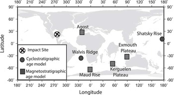
The data come from published counts of nannofossil abundance in samples from five deep sea sediment cores and one shelf section (Fig. 1) (Pospichal and Wise Reference Pospichal and Wise1990; Pospichal and Bralower Reference Pospichal and Bralower1992; Pospichal Reference Pospichal1995; Arney and Wise Reference Arney and Wise2003; Bown Reference Bown2005; Bernaola and Monechi Reference Bernaola and Monechi2007; Jiang et al. Reference Jiang, Bralower, Patzkowsky, Kump and Schueth2010). This dataset is a subset of the much larger K/Pg nannofossil database compiled by Jiang et al. (Reference Jiang, Bralower, Patzkowsky, Kump and Schueth2010). The six sites lie in both hemispheres and are from all of the major ocean basins. These sites were selected because they have high resolution age control based on orbital stratigraphy and magnetostratigraphy. Unfortunately this constraint excluded a number of shelf sections with superb nannoplankton records across the K/Pg boundary, including El Kef, Tunisia, and Brazos, Texas.
Location map and type of age control for each site. Map is modified from paleogeographic reconstruction of 65.5 Ma generated using the ODSN plate reconstruction (www.odsn.de/odsn/services/paleomap/paleomap.html).

Taxa were grouped as survivors, new Paleogene species, and short lived “bloom” taxa. Survivors are considered taxa which cross the K/Pg boundary and either increase in abundance or maintain abundance over the interval, compared to taxa considered to have become extinct which rapidly drop in abundance at the boundary (Supplementary Appendix) (Percival and Fischer Reference Percival and Fischer1977; Perch-Nielsen Reference Perch-Nielsen1985; Pospichal Reference Pospichal1994, Reference Pospichal1996). New Paleogene taxa are those that have distinct first occurrences in the Paleogene and are unobserved in the Maastrichtian. We define the bloom taxa as those with peaks in abundance greater than 20% of the assemblage that lasted only a few hundred thousand years. All samples in the analysis were originally counted to approximately 300 specimens, including Cretaceous species in Paleogene samples. We consider Cretaceous species as those that have not been identified as survivors and have distinct, dramatic declines in abundance at the K/Pg boundary (e.g., Perch-Nielsen Reference Perch-Nielsen1985; Pospichal, Reference Pospichal1996; Bown Reference Bown2005). These Cretaceous specimens were removed from the Paleogene samples because early Paleocene assemblages often contain reworked extinct Cretaceous taxa (e.g., MacLeod et al. Reference MacLeod, Huber and Fullagar2001; Minoletti et al. Reference Minoletti, de Rafelis, Rendard, Gardin and Young2005). Calcispheres, including the genus Thoracosphaera, are calcareous dinoflagallete cysts that often are counted along with nannoplankton in early Paleocene assemblages. These taxa were also removed from the dataset because they are biologically unrelated to other nannoplankton, and, in addition, they potentially mute significant trends due to their abundance (e.g., Perch-Nielsen Reference Perch-Nielsen1985). The remaining counts, which no longer totaled 300, were then used for all analyses. Several species were combined into genera to standardize taxonomy between the different workers. Finally, prior to all statistical analysis we converted the nannofossil count data into a percentage of the entire assemblage then log transformed the percentage data to lessen biases caused by dominance of individual taxa.
Age Models
Cyclostratigraphic age models tuned to 100 Kyr orbital eccentricity cycles provide the most precise method of age control in the Paleocene. The use of these age models allows us to determine and correlate biostratigraphic datums with precision and to compare short term evolutionary trends between sites. Cyclostratigraphic age models have been developed for Ocean Drilling Program Sites 1210 (Shatsky Rise) and 1262 (Walvis Ridge) (Westerhold et al. Reference Westerhold, Röhl, Raffi, Fornaciari, Monechi, Reale, Bowles and Evans2008). For these sites, we used the “option 2” tuning of Westerhold et al. (Reference Westerhold, Röhl, Raffi, Fornaciari, Monechi, Reale, Bowles and Evans2008) because this best approximates the age of the K/Pg boundary determined from radiometric dating (e.g., Kuiper et al. Reference Kuiper, Deino, Hilgen, Krijgsman, Renne and Wijbrans2008). The age of each sample at Shatsky Rise and Walvis Ridge was then determined assuming constant sedimentation between the 100 Kyr short eccentricity cycles.
The other four sites we selected, ODP Sites 690 (Maud Rise), 761 (Exmouth Plateau), 1138 (Kerguelen Plateau), and the Agost shelf section have magnetostratigraphic age control (Groot et al. Reference Groot, de Jonge, Langereis, ten Kate and Smit1989; Spieß Reference Spieß1990; Galbrun Reference Galbrun1992; Antretter et al. Reference Antretter, Inokuchi and Zhao2003). We constructed less precise age models for these four sites with the assumption of constant sedimentation rates between magnetic reversals (Supplementary Appendix). The lack of finer resolution age control decreased the precision of correlation and limited interpretation of evolutionary trends. Therefore, while we used the global dataset to make important inferences on the overall recovery of nannoplankton from the K/Pg extinction, we focused on the Shatsky Rise and Walvis Ridge sites for problems that required orbital age resolution.
Nannofossil Datums
To compare the timing of first occurrences, we calculated precise nannofossil originations for the two sites with cyclostratigraphic age control, Shatsky Rise (Site 1210) and Walvis Ridge (Site 1262). The original data for these sites were assemblage counts taken from the Jiang et al. (Reference Jiang, Bralower, Patzkowsky, Kump and Schueth2010) database. The slides used for counts often have few specimens per field of view to make counting easier (Bown and Young Reference Bown and Young1998), and rare species can be easily overlooked. To determine originations with greater precision, we made thicker smear slides with more specimens per field of view from all of the original Shatsky Rise samples (ODP Hole 1210A) and Walvis Ridge samples from ODP Hole 1262B that were depth equivalent to the original samples from Hole 1262C. Each slide was observed using cross polarized light at 1600× magnification for at least two entire slide traverses (generally 50–100 fields of view). This provided us with a more accurate placement of the origination to compare with the datum derived from the count data. We determined the first occurrence datums for taxa in the key lineages: Futyania, Neobiscutum and Prinsius (Prinsius clade), Cruciplacolithus primus and Cr. intermedius (Cruciplacolithus clade), and Coccolithus (Coccolithus clade).
Even with a more intense investigation of thicker slides, the datums that are found with this technique are still likely not the first true occurrence of the taxa. Originations are subject to local range offset, the difference in age between the observed first occurrence and the true origination. Local range offset is a result of poor preservation or infrequent observation of a species in the earliest part of its true range, where it is often the rarest (e.g., Holland and Patzkowsky Reference Holland and Patzkowsky2002; Patzkowsky and Holland Reference Patzkowsky and Holland2012), and potentially sediment reworking and remixing. The interpretation of diachronous first occurrences could only represent a difference in the extent of local range offset at different locations. We account for errors caused by local range offset with the use of the Probable Datum Method (PDM) (Schueth et al. Reference Schueth, Keller, Bralower and Patzkowsky2014). The PDM models the processes that create an observed abundance from the original environmental abundance: the preservation of the fossil and the count of the fossil by a paleontologist. It then takes this model and inverts it, moving from our observed abundance to a likely range of original abundance of the species. With this original abundance it determines a likely age of first or last occurrence in the environment. This age is independent of our observed fossil datum and acts as an unbiased estimate of true first occurrence. Therefore it allows us to compare originations between sites without interpreting differences in preservation or observation as true biologic signals.
The PDM was run on the six taxa of interest for both Walvis Ridge and Shatsky Rise (see Schueth et al. in 2014 and Supplementary Appendix). The PDM statistically produces a probability distribution for the true age of first occurrence, rather than a single likely age. While the true first occurrence can be any age in this distribution, we determined the mean value of the distribution to assess the most likely age of first occurrence. After age distributions were produced for both sites, the PDM randomly samples the distribution at each site. The difference in age between these samples is an estimate of the synchrony of the first occurrence. This process is repeated 1000 times to generate a probability distribution of the difference in age between the sites. This distribution is used to test the null hypothesis that the first occurrence was synchronous between sections. We assume that datums are synchronous if they are less than the resolution of our age model, in this case one eccentricity cycle (100 Kyr) (Westerhold et al. Reference Westerhold, Röhl, Raffi, Fornaciari, Monechi, Reale, Bowles and Evans2008). The proportion of the age difference distribution less than 100 Kyr provides a p-value for the null hypothesis of a synchronous first occurrence (Schueth et al. Reference Schueth, Keller, Bralower and Patzkowsky2014). The null hypothesis can be rejected once the p-value reaches a desired level of confidence, and the first occurrences can then be considered to be diachronous. A more comprehensive overview of the PDM and its application is provided in Schueth et al. (Reference Schueth, Keller, Bralower and Patzkowsky2014).
Diversity
Both species richness, or total number of species, and Shannon diversity, which incorporates species richness and evenness, were calculated for the original data from Shatsky Rise (Bown Reference Bown2005) and Walvis Ridge (Bernaola and Monechi Reference Bernaola and Monechi2007; Jiang et al. Reference Jiang, Bralower, Patzkowsky, Kump and Schueth2010). These calculations also excluded calcipheres (Thoracosphaera) and reworked Cretaceous species. The diversity of samples from approximately the last 100 Kyr of the Maastrichtian was also calculated to compare diversity in the pre extinction interval to that in the recovery interval. Because we are interested in short term diversity trends and we wish to compare diversity directly between sites, we calculated diversity only for the sites with cyclostratigraphic age control (Shatsky Rise and Walvis Ridge).
Cluster Analysis
We performed separate cluster analyses on species and samples from all sites. The analyses were done on all samples in our global database to determine how nannoplankton assemblages changed through time. The cluster analyses were run on the transformed abundance data with a Bray Curtis distance metric and Ward’s linking method using the “agnes” function in the “cluster” package in R software (Maechler et al. Reference Maechler, Rosseeuw, Struyf, Hubert and Hornik2012; R Development Core Team 2013).
Nonmetric Multidimensional Scaling
To determine global trends in recovery we performed a Nonmetric Multidimensional Scaling (NMS) analysis on the transformed nannofossil dataset. The NMS analysis is a technique that ordinates the data in reduced variable space using the ranked distance between samples. We chose to apply NMS over other ordination methods because it uses ranked distance, which eliminates many biases and assumptions of the data inherent in other methods (Clarke Reference Clarke1993). The ordination uses a Bray Curtis distance, and was run with the metaMDS algorithm in the vegan package in R (Oksanen et al. Reference Oksanen, Blanchet, Kindt, Legendre, Minchin, O’Hara, Simpson, Solymos, Stevens and Wagner2013; R Development Core Team 2013). This algorithm also performs a Principle Components Analysis rotation of the result and adds species into the sample NMS space after the fact with a weighted averaging function that relates species abundance to the NMS dimensions. It therefore allows us to interpret both the samples and taxa in the same ordination space.
Results
Focused Study of North Pacific and South Atlantic Sites
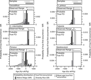
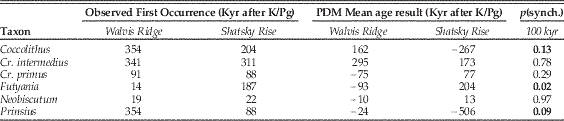
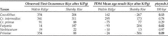
Our study initially focused on the two sites with the most comprehensive age control, Shatsky Rise in the North Pacific, and Walvis Ridge in the South Atlantic (Fig. 1). For simplicity, we assumed that any observed trends in the nannoplankton recovery at these sites are representative of the entire North Pacific and South Atlantic Oceans. We determined the first observed occurrence based on smear slide observations at both sites (Fig. 2; Supplementary Appendix). Mai et al. (Reference Mai, Speijer and Schulte2003) observed several specimens of Cr. primus and Neobiscutum in Maastrichtian samples, indicating these taxa may have originated before the boundary. Thus, their Paleocene first occurrences are site specific stratigraphic horizons that do not carry evolutionary significance. The PDM application to each taxon at both sites produced histograms of the distribution of estimated true origination age (Fig. 2). For each taxon, we report the age of first occurrence in the original data, the age of first observed occurrence, the mean value of likely true first occurrence from the PDM, and the probability that the origination was synchronous between Shatsky Rise and Walvis Ridge (Table 1; Fig. 2). Given uncertainty in some model parameters, especially preservation, we feel that it is safe to reject our null hypothesis of a synchronous first occurrence with a p-value ≤0.15. With this cutoff, we can reject the hypothesis of a synchronous first occurrence for Futyiania (p-value < 0.05), Prinsius (p<0.01), and Coccolithus (p<0.15). We cannot rule out a synchronous origination for Cr. intermedius or Neobiscutum, both of which have p-values >0.75.
First occurrence datums for all six taxa for Shatsky Rise (North Pacific, light gray) and Walvis Ridge (South Atlantic, dark gray). We illustrate samples collected at the top of each column. We show the histograms of the age of probable true first occurrence determined from the PDM (Schueth et al. Reference Schueth, Keller, Bralower and Patzkowsky2014) along with the range of observed occurrence (horizontal vertical lines) and the observed first occurrence (stars). The y-axis represents the probability of each age being the true first occurrence. We also illustrate the mean value of each distribution (solid vertical lines).

Observed first occurrence in the count abundance data of each taxon for Shatsky Rise (Bown Reference Bown2005) and Walvis Ridge (Bernaola and Monechi Reference Bernaola and Monechi2007), the mean of the PDM results and the p-value that for the hypothesis that the originations were synchronous p(synchronous), as derived from the PDM (Schueth et al. Reference Schueth, Keller, Bralower and Patzkowsky2014). Datums are considered synchronous if they fall within 100 Kyr between sites. We consider a p(synchronous) value ≤0.15 (in bold) as a cutoff to reject the null hypothesis of synchronous first occurrence between sites.
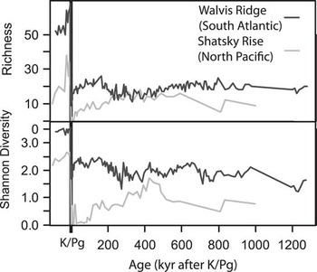
Both sites experienced a sharp drop in species richness and Shannon diversity at the boundary, but both diversity metrics rebounded at Walvis Ridge almost immediately (Fig. 3). This quick rebound was followed by little to no significant changes in both richness and Shannon diversity for the remainder of the recovery interval, and diversity was still muted compared to the Cretaceous. Shatsky Rise was characterized by a much slower recovery. Richness did not approach Walvis Ridge levels until approximately 250 Kyr after the boundary, and Shannon diversity was not comparable until 400 Kyr after the extinction. This discrepancy in the recovery of diversity was also noted by Jiang et al. (Reference Jiang, Bralower, Patzkowsky, Kump and Schueth2010).
Species richness (top) and Shannon diversity (bottom) for nannoplankton at Shatsky Rise (light gray) and Walvis Ridge (dark gray). Age is given as Kyr after the K/Pg boundary. Note the collapse in diversity at the boundary and the rapid rebound followed by long plateau in diversity at Walvis Ridge. Shatsky Rise has a much slower recovery in diversity.

Global Nannoplankton Recovery Results
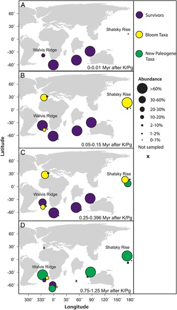
We inferred general trends of nannoplankton recovery from a more global compilation of nannofossil data despite the lack of precise age control. We assumed the few sites we have in our dataset to represent either entire oceans or hemispheres for the sake of simplicity. We plotted the abundance of the three primary groups of post extinction nannoplankton, survivors, bloom taxa, and new Paleogene taxa, at each site through the recovery interval. Average abundances of each group for four time bins are plotted for all six sites (Fig. 4A–D). All time bins are shown in the Supplementary Appendix. Immediately after the extinction (i.e., <10 Kyr), nannoplankton abundance was very low at the Northern Hemisphere sites, but survivors were very abundant at the Southern Hemisphere sites (Fig. 4A). Within 0.05–0.15 Myr after the boundary, there were distinct differences between Northern and Southern Hemisphere assemblages where bloom taxa dominated the Northern Hemisphere while survivors were most abundant in the Southern Hemisphere (Fig. 4B). Recovery taxa first appeared and become abundant at Shatsky Rise (Fig. 4C), then steadily dispersed into the Southern Hemisphere. It was not until after 0.25–0.40 Myr that new Paleogene assemblages were globally abundant (Fig. 4D).
Paleogeographic map of K/Pg samples (see Fig. 1) showing average abundance of different nannofossil groups in various windows of time. Size of circle indicates abundance and color taxonomy (purple=survivors; yellow=bloom taxa; green=new Paleogene taxa). Here we show four time windows (in Myr after the boundary) labeled A–D (A=0–0.01 Myr; B=0.05–0.15 Myr; C=0.25–0.396 Myr; D=0.75–1.25 Myr). Notice the difference in assemblages between North and South Hemispheres and the slow spread of New Paleogene taxa. Paleogeography modified from 65.5 Ma ODSN plate reconstruction (www.odsn.de/odsn/services/paleomap/paleomap.html). A full reconstruction is given in the Supplementary Appendix.

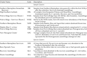
We provide a brief overview of our sample and species clusters from the cluster analysis in Table 2 and a more thorough discussion of the cluster analysis results, including dendrograms, in the Supplementary Appendix. We interpreted eight sample clusters and four taxon clusters or groups (Table 2). Each of these clusters correlates to distinct trends in abundance. We use the patterns observed in the cluster analysis to understand the structure and evolution of nannoplankton assemblages in the recovery interval.
Summary of cluster analysis results with full cluster analysis description and dendrogram shown in the Supplemental Materials. Here we describe the eight sample clusters and four taxon clusters, and a brief description of each cluster is provided.

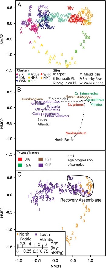
The results of the NMS are shown as plots of samples and taxa in NMS space with the first NMS dimension, NMS1, plotted against the second, NMS2 (Fig. 5). Samples and taxa were color coded by their cluster grouping. The samples from the Northern Hemisphere sites (Shatsky Rise and Agost) show clear differences from the Southern Hemisphere sites in the NMS results, primarily along NMS2 (Fig. 5A). The NMS results for the taxa (Fig. 5B), suggest this difference is due to assemblage differences between the Southern Hemisphere sites, which are mostly comprised of taxa in the Southern Hemisphere Survivors cluster, whereas the Northern Hemisphere sites are dominated by the Bloom Assemblage cluster (Table 2). In younger samples, both hemispheres plot together in the NMS, as in Jiang et al. (Reference Jiang, Bralower, Patzkowsky, Kump and Schueth2010), and are mainly comprised of Cr. intermedius, Coccolithus and Prinsius (Fig. 5). We define the area of the NMS plots with high positive values of NMS1 and NMS2 characterized by samples abundant with these taxa, as the “recovery assemblage.” Shatsky Rise samples are characterized by this recovery assemblage much earlier than Walvis Ridge samples as shown by the age progression of samples in NMS space (Fig. 5C).
The NMS results. A, Samples plotted in NMS space where the letter designates the site the sample came from and the color the sample cluster (see Table 2). B, The taxa plotted in NMS space. Here the color of each taxon represents its position in the species cluster analysis (Table 2). C, The age progression of Shatsky Rise and Walvis Ridge samples in NMS space. Also illustrated is the area of NMS space where samples are dominated by new Paleogene taxa (the Recovery Assemblage). Samples from Shatsky Rise (North Pacific Ocean) reach this space much earlier than do samples from Walvis Ridge (South Atlantic Ocean).

Discussion
In the wake of the mass extinction, and for several hundreds of thousands of years afterwards, Northern Hemisphere locations were characterized by higher abundances of bloom taxa and Southern Hemisphere locations were characterized by higher abundances of surviving taxa (e.g., Jiang et al. Reference Jiang, Bralower, Patzkowsky, Kump and Schueth2010). Here we explore the implications of these geographic differences on the evolutionary record of nannoplankton, and attempt to understand how new taxa dispersed and became dominant in global assemblages. We first interpret the high resolution stratigraphic comparison between assemblage data from Shatsky Rise and Walvis Ridge. We then include the lower resolution, global database to explore the hypothesis that the recovery of nannofloral assemblages was ecologically, and not environmentally, constrained.
Nannoplankton Evolution after the K/Pg Mass Extinction
Calcareous nannoplankton diversified dramatically in the aftermath of the K/Pg mass extinction. Three families (Coccolithaceae, Prinsiaceae and Zygodiscaceae) and seven genera (Biantholithus, Coccolithus, Cruciplacolithus, Hornibrookina, Lanternithus, Neochiastozygus, Prinsius) were established within the first Myr of the Paleocene (Aubry Reference Aubry1998; Bown et al. Reference Bown, Lees and Young2004). A significant proportion of this radiation was the consequence of the post extinction proliferation of Neobiscutum and Cruciplacolithus primus, two taxa that either arose immediately after the extinction or were very rare and restricted to shelf settings in the latest Cretaceous (Mai et al. Reference Mai, Speijer and Schulte2003). Here we focus on the six abundant Paleocene taxa: Coccolithus, Cr. primus, Cr. intermedius, Futyania, Neobiscutum, and Prinsius. Accurate determination of the age of first occurrence of these taxa in local sections can pinpoint where species first appeared and how their ranges expanded. We focus the discussion on the first million years after the K/Pg boundary. For interpretation of regional recovery patterns we assume the few study sites represent ocean wide trends.
Cruciplacolithus primus and Neobiscutum likely had synchronous first occurrences between Shatsky Rise and Walvis Ridge according to the PDM results (Table 1; Fig. 2). This, coupled with their appearance within the first 100 Kyr after the extinction, supports previous interpretations that these taxa were survivors that rapidly expanded in the immediate wake of the impact (Mai et al. Reference Mai, Speijer and Schulte2003). Futyania appeared first at Walvis Ridge (Table 1; Fig. 2), and its early first occurrence (14 Kyr after K/Pg) suggests that it was also a survivor or that it evolved immediately following the mass extinction. The first occurrences of Coccolithus and Prinsius were especially significant as these two genera are known with certainty to originate after the mass extinction, and, moreover, their descendants became dominant members of Paleocene assemblages (e.g., Bown et al. Reference Bown, Lees and Young2004). Coccolithus and Prinsius appeared first in the North Pacific Ocean (Shatsky Rise), then 150 and 266 Kyr later in the South Atlantic (Walvis Ridge), respectively (Table 1; Fig. 2). There is high confidence from the PDM results that these originations were diachronous: synchrony can be ruled out for both originations with the p-value cutoff ≤0.15 (Table 1). Age model error could lead to the observed diachrony (e.g., Hull et al. Reference Hull, Norris, Bralower and Schueth2011); however, there is little evidence for such error, and some of the observed diachrony is greater than age model resolution (i.e., >100 Kyr).
The final new taxon under consideration, Cruciplacolithus intermedius, differs from Coccolithus and Prinsius in appearing in the South Atlantic and Pacific at the same time (Table 1; Fig. 2). This synchronous first occurrence is supported in the PDM results, with a p-value=0.78 (see Results). This species originated from C. primus, which was well established in the South Atlantic. Coccolithus and Prinsius were new genera in the Danian and thus their originations were potentially controlled by different biological and ecological factors from C. intermedius. Moreover, C. intermedius is far less abundant than both Coccolithus and Prinsius.
The shapes of the probability distributions for true first occurrence vary by taxa as a function of their abundance and preservation potential (as explained in the PDM parameters in the Supplementary Appendix). Taxa with very narrow probability distributions, such as Neobiscutum and Futyania, had sharp increases in abundance after their observed first occurrence. Therefore the shape of the distributions is largely a result of the logistic model fit of the PDM to the original count data (Schueth et al. Reference Schueth, Keller, Bralower and Patzkowsky2014). Of significance, the PDM shows a wider range in uncertainty of the probable true first occurrence for taxa with long periods of sporadic, low abundance following the first occurrence, where the taxa may have been poorly preserved, reworked, or unobserved at its low abundance. We illustrate the logistic model fits and explain this further in the Supplementary Appendix.
There is also a possibility that a step improvement in preservation occurred at the boundary, as seen by a decrease in foraminiferal fragmentation (e.g., D’Hondt Reference D’Hondt2005). This was not incorporated into our application of the PDM, where we assumed approximately constant preservation through time. However, if such a change in preservation occurred, the PDM results would shift the distribution of the histograms earlier, supporting the possibility that the early Paleocene taxa originated in the Maastrichtian but were not preserved. Therefore our assumption of constant preservation across the boundary increases the likelihood that most originations occurred close to or after the K/Pg boundary. We ran a sensitivity test on the PDM to confirm this scenario by adding a step change in preservation at the boundary (Supplementary Appendix).
Following the mass extinction, species richness at Shatsky Rise was fairly low with less than ten species in assemblages for almost 250 Kyr (Fig. 3). During the same interval, Walvis Ridge had much higher species richness with 20 to 30 species present (Fig. 3). At Walvis Ridge, diversity (as measured by both species richness and Shannon diversity) rapidly rebounded and plateaued within 30 Kyr after the extinction. These diversity metrics did not change significantly for the remainder of the sampled interval (Fig. 3). The initial diversification in the South Atlantic Ocean was almost entirely due to a rapid increase in abundance of surviving genera, rather than speciation (Supplementary Appendix). These survivor taxa, primarily Biscutum, Cyclagelosphaera, and Markalius, comprised <1% of taxa in Cretaceous samples but 20–40% in the first 100 Kyr after the K/Pg boundary. Zeugrhabdotus sigmoides was absent in all uppermost Maastrichtian Walvis Ridge samples but became >40% of the assemblage 60 Kyr after the boundary. We removed taxa that are commonly ascribed as “Cretaceous taxa” (e.g., Perch-Nielsen Reference Perch-Nielsen1985; Bown Reference Bown2005) in Paleocene aged samples as these are likely reworked (see Methods). This may have inflated the relative abundance of survivors. However, the observed increase in survivor abundance at Walvis Ridge remains in the original dataset that includes Cretaceous taxa. For example, even with Cretaceous taxa included, Z. sigmoides reached >20% of the Walvis Ridge assemblage within 100 Kyr after the extinction. We postulate that these rare survivors rapidly dispersed from extinction refugia into the South Atlantic Ocean immediately following the mass extinction.
Global Patterns of Nannofloral Recovery
Key new Paleogene taxa (i.e., Coccolithus, Prinsius) appeared at Shatsky Rise before Walvis Ridge (Table 1; Fig. 2), and rose to dominate assemblages there 250–350 Kyr after the extinction. Here we compare the first occurrences of these genera on a global basis. Based on magnetochronology of the other sites in our dataset, Coccolithus and Prinsius also appeared in the North Pacific 50–300 Kyr before they did at sites in the Indian and Southern Oceans. The first appearance of Coccolithus is not observed at the Agost section, the only Tethyan site in our database, even though the youngest sample is about 260 Kyr after the K/Pg boundary. Prinsius appeared after 200 Kyr at Agost, but never became as abundant as it did in the sampled section at Shatsky Rise. This may indicate Coccolithus and Prinsius did not appear synchronously over the entire Northern Hemisphere, and that their origination was focused in the North Pacific Ocean. However, we lack age control in other Tethyan or North Atlantic Ocean sections to confirm this conclusion.
The new taxa were rare at all of the Southern Hemisphere sites for up to 500 Kyr after the boundary (Jiang et al. Reference Jiang, Bralower, Patzkowsky, Kump and Schueth2010; Fig. 4C,D). These new Paleogene taxa were also rare for most of the sampled Danian in the North Atlantic and Tethyan sections (Jiang et al. Reference Jiang, Bralower, Patzkowsky, Kump and Schueth2010). In the Northern Hemisphere sites, outside of Shatsky Rise, bloom taxa, especially Braarudosphaera, C. primus, and Neobiscutum, dominate assemblages after the extinction. The same survivors seen at Walvis Ridge also dominate all Southern Hemisphere sites. These taxa rapidly expanded in all Southern Hemisphere sites and were abundant there for hundreds of thousands of years after the extinction (Fig. 4), but were rare to absent for most of the sampled sections at all sites in the North Atlantic and Tethys (Jiang et al. Reference Jiang, Bralower, Patzkowsky, Kump and Schueth2010). Therefore, the South Atlantic assemblage dominated by survivors is interpreted as a hemispheric phenomenon.
The cluster analysis shows that global assemblages were notably heterogeneous during the recovery. In the earliest Danian samples (i.e., from 0 to 400 Kyr after the boundary), clusters primarily separate Northern and Southern Hemisphere samples based on the dominance of bloom taxa versus survivors (Table 2; Supplementary Appendix). Shatsky Rise, Walvis Ridge, and Exmouth Plateau samples do not cluster together until 400 Kyr to 1.2 Myr after the boundary when samples become dominated by species in the Recovery Assemblage Cluster, which contains abundant new Paleogene taxa including Coccolithus and Prinsius (Table 2; Supplementary Appendix). Therefore, the expansion of these two genera from their center of origination in the North Pacific into other oceans was a key step in the initial recovery of nannoplankton. The transition from global heterogeneity to a homogeneous assemblage comprised primarily of new taxa is also shown in the NMS results. The new Paleogene assemblage rose to dominance first in the North Pacific, where samples from Shatsky Rise plot in the “recovery assemblage” portion of NMS space (i.e., high positive values of NMS1 and NMS2) 200–300 Kyr before the other sites (Fig. 5).
Both our focused study of Shatsky Rise and Walvis Ridge, and the more global investigation, can be used to investigate the hypothesized role of regional incumbency in the observed geographic heterogeneity of nannoplankton assemblages in the earliest Paleocene. We have made two key observations: (1) survivors rapidly expanded at all Southern Hemisphere sites, and (2) taxa that make up the recovery assemblage appeared and became abundant first at Shatsky Rise in the Pacific but not at sites in the Atlantic and Tethys. This is a distinct biogeographical pattern that must be explained either through a unique environmental difference between the North Pacific and the rest of the oceans or through ecologic constraints on the dispersal of new taxa.
There likely were no climatic effects of the bolide impact that would have lasted 300–400 Kyr after the boundary (e.g., Toon et al. Reference Toon, Zahnle., Morrison, Turco and Covey1997; Pope et al. Reference Pope, Baines, Ocampo and Ivanov1997; Pope Reference Pope2002). Primary productivity recovered almost immediately after the impact (Sepúlveda et al. Reference Sepúlveda, Wendler, Summons and Hinrichs2009); however, the efficiency of the biological pump (in the sense of Hilting et al. (Reference Hilting, Kump and Bralower2008)) was not restored to pre extinction levels for hundreds of thousands of years or longer. Moreover, Jiang et al. (Reference Jiang, Bralower, Patzkowsky, Kump and Schueth2010) showed Northern Hemisphere sites had a more significant initial collapse in the surface to deep ocean carbon isotopic gradient, perhaps suggesting that the biologic pump was less efficient immediately after the impact. This could explain the initial hemispheric differences of nannoplankton assemblages.
The recovery of the biological pump took place in two steps as indicated by the carbon isotopic gradient: a first initial recovery and a final recovery (e.g., D’Hondt et al. Reference D’Hondt, Donaghay, Zachos, Luttenberg and Lindinger1998). The initial recovery may have been geographically variable, although its timing, about 400 Kyr after the boundary, has been shown to be essentially synchronous between Shatksy Rise and Walvis Ridge (Coxall et al. Reference Coxall, D’Hondt and Zachos2006). The final recovery was a globally synchronous event about 3 Myr after the extinction (e.g., D’Hondt Reference D’Hondt2005; Coxall et al. Reference Coxall, D’Hondt and Zachos2006). These patterns in biological pump recovery do not match the observed patterns in the development and dispersal of the recovery assemblage. Ecological constraints on the development and dispersal of the recovery assemblage may better explain the observed patterns.
The Effect of Regional Incumbency on Nannofloral Recovery
Nannoplankton assemblages should be relatively homogenous as plankton disperse throughout the oceans within a few hundred years (Norris Reference Norris2000), and geographical and environmental barriers are not known to prevent the dispersal of plankton today or at other times in the past (Sexton and Norris Reference Sexton and Norris2008; Cermeño and Falkowski Reference Cermeño and Falkowski2009). Indeed, pre extinction nannoplankton assemblages were globally homogeneous, primarily differing between high and low latitudes (e.g., Worsley and Martini Reference Worsley and Martini1970; Thierstein Reference Thierstein1981; Huber and Watkins Reference Huber and Watkins1992; Lees Reference Lees2002). The key event of the nannoplankton recovery was the origin and dispersal of the Coccolithus and Prinsius clades from the North Pacific, so we must understand why it took so long for these taxa to become globally abundant.
Survivors, especially the eutrophic genera Biscutum, Cyclagelosphaera, Markalius, Neocrepidolithus, and Zeugrhabdotus, became rapidly abundant at all Southern Hemisphere sites within the first 15–30 Kyr after the extinction, but were rare to absent at all Northern Hemisphere sites (Jiang et al. Reference Jiang, Bralower, Patzkowsky, Kump and Schueth2010). A prolonged plateau in diversity followed the increase in abundance of survivors at Walvis Ridge (Fig. 3). After their first appearance at Southern Hemisphere sites, new taxa such as Coccolithus and Prinsius remained rare for some time (Fig. 4; Supplementary Appendix). Modern ecological studies have shown that invaders often enter into ecosystems with established incumbency but remain rare for extended periods of time (e.g., Tilman Reference Tillman2004), in line with our observations. We hypothesize that survivors developed into a regionally incumbent assemblage in the Southern Hemisphere Oceans that limited diversification and the dispersal of the new taxa that appeared first in the North Pacific. The lack of early expansion of Coccolithus and Prinsius at Agost is interesting as there was not a large survivor assemblage there. Instead Agost assemblages were dominated by bloom taxa for the entire interval perhaps indicating a harsher local environment in the Tethys, or that shelf sections in general were more suitable for bloom assemblages for at least the first 300 Kyr after the extinction.
The North Pacific Ocean was a center of origination for new taxa, and an assemblage of dominant new Paleogene taxa first developed there after the environment became more hospitable. It then took hundreds of thousands of years for the new assemblage to become abundant globally. The incumbent survivor assemblage acted as a biological barrier in the Southern Hemisphere, effectively preventing the dispersal of these new taxa. The significant diachrony of first occurrences, and the delay in the dispersal of new taxa between hemispheres, argues that regional incumbency was the primary control on early nannoplankton recovery.
While incumbency hypothetically should influence planktonic ecosystems (e.g., Hanson et al. Reference Hanson, Fuhrman, Horner-Devine and Martiny2012), there has not yet been any direct evidence of prolonged, geologic scale, incumbent effects in marine phytoplankton. Incumbency itself seems hard to maintain in pelagic ecosystems where abundance is very seasonal as a result of processes such as grazing and because individuals are so easily dispersed between basins. We speculate that in the highly heterogeneous post extinction environment with dominant survivors forming large populations regionally, incumbency became established even at times of the year when populations dwindled. Despite seasonal fluctuations in abundance of the incumbents, the rarity of new taxa would not be enough to displace such a large initial population base; especially considering these new taxa would also be subject to seasonal fluctuations in abundance.
The eventual transition to a globally homogeneous new Paleogene assemblage took place only after survivor abundance began to decline in the Southern Hemisphere Oceans around 350 Kyr after the K/Pg boundary at Walvis Ridge and 350–400 Kyr after the boundary at the Indian Ocean sites (Fig. 4). The decline in the regionally incumbent survivors may have been a result of the recovery of the biologic pump and decline in surface water nutrients. The initial recovery of the carbon isotopic gradient around 300–400 Kyr after the K/Pg boundary (e.g., Adams et al. Reference Adams, Mann and D’Hondt2004; D’Hondt Reference D’Hondt2005; Coxall et al. Reference Coxall, D’Hondt and Zachos2006) was nearly the same time survivor abundance declined and the recovery assemblages expanded. We therefore postulate that, while the recovery of the biologic pump was not responsible for the observed paleogeographic patterns of nannoplankton recovery, it may have been a factor that led to the end of regional incumbency. As the biologic pump began to recover and nutrient cycling became more efficient, the surface oceans became less favorable for the eutrophic survivor assemblages and more favorable for the recovery assemblage. A decline in surface water nutrients facilitated both the loss of regional incumbency in nannoplankton and the gain of photosynthetic endosymbionts in planktonic foraminifera, which would also explain the coincidental timing of the δ13C gradient recovery and the recovery of both groups.
The carbon isotopic gradient recovery has been ascribed directly to the transition from assemblages dominated by calcareous dinoflagellates to the nannofloral recovery assemblage (e.g., Alegret et al. Reference Alegret, Thomas and Lohmann2012). However, this hypothesis is not supported by our observations, as the gradient recovery occurs several hundred thousand years after calcareous dinoflagellates decline in abundance. Alternatively, we postulate that higher benthic foraminiferal and fish teeth accumulation rates in the North Pacific (Alegret and Thomas Reference Alegret and Thomas2009; Sibert et al. Reference Sibert, Hull and Norris2014) are consistent with less efficient regional biological pumping, which would result in a higher food supply in the surface ocean and export productivity to the sea floor (Hilting et al. Reference Hilting, Kump and Bralower2008).
Incumbency has been shown as an important ecological force in the establishment of fossil species in new environments (e.g., Gilinsky and Bamback Reference Gilinsky and Bamback1987; Vermeij Reference Vermeij1991, Reference Vermeij2005; Sheehan Reference Sheehan2008). While incumbency has been used to explain rapid diversification following mass extinction (e.g., Jablonski Reference Jablonski1998, Reference Jablonski2008), we have shown that the global disparity in assemblages in the initial recovery can cause regional incumbent effects that are equally as important (Sheehan Reference Sheehan2008). Our results suggest that biologic competition from regionally incumbent taxa is an important mechanism that mediates the distribution and establishment of new taxa of nannoplankton, and likely all marine life, in the initial recovery from mass extinction.
Conclusions
We determined where key lineages of new Paleogene nannoplankton taxa evolved and how they became globally dominant. Regional incumbency of endemic survivors played a significant role in the global patterns of recovery of nannoplankton. We conclude:
1. Survivors rapidly expanded into all Southern Hemisphere sites and established a regionally incumbent assemblage. These endemic, incumbent survivors may have limited diversification and acted as a biological barrier that prevented the global dispersal of new Paleogene taxa.
2. The key Paleogene taxa, Coccolithus and Prinsius, appeared in the North Pacific Ocean before the South Atlantic. This was perhaps due to a lack of competition from survivors in the North Pacific.
3. Regional incumbency of eutrophic survivors may have ended when nutrient concentrations in the surface oceans decreased, possibly due to the recovery of biologic pump efficiency. Only following the decline in survivor abundance did new Paleogene taxa become abundant at all sites. This suggests that competition from survivors was as an important control on early Paleocene nannoplankton evolution.
Acknowledgements
This work was funded through National Aeronautics and Space Administration Exobiology grant NNH10DA001N-EXG to T. Bralower and National Natural Science Foundation of China Project 41372034 to S. Jiang. This manuscript was greatly strengthened with reviews from P. Hull and two anonymous reviewers. We thank K. Keller and E. Post at Pennsylvania State University for comments on a previous draft of this manuscript.
Supplementary Material
Supplemental materials deposited at Dryad: 10.5061/dryad.676tf