1 Introduction
With every realization of a turbulent field being unique, scaling laws are commonly sought when searching for insight or for furthering the reach of flow statistics to higher Reynolds numbers and even different geometries. Scaling is equally important in direct numerical simulation (DNS) of turbulence studies, which have been widely used at relatively low Reynolds numbers but now include flows well clear of the transition threshold. For turbulence through a straight square duct, the subject of the present paper, the search for scaling laws must be deferred to Reynolds numbers based on the friction velocity and duct half-side beyond 600, because below this value, the flow is changing in an essential way; this is reflected in its inbuilt turbulence-sensitive mark, the mean secondary flows.
The DNS data in this paper follow the changes in the mean and turbulent fields as the friction velocity Reynolds number is increased from 157 up to 861 with the main interest in the highest value. There is no recent experimental work spanning the Reynolds number range that captures this non-laminar transition phase of the square duct flow, and the thesis of Hoagland (Reference Hoagland1960) does not contain sufficiently detailed data for such an investigation. There is, however, a recent DNS study of Zhang et al. (Reference Zhang, Trias, Gorobets, Tang and Oliva2015) where the highest friction velocity Reynolds number is 600, but the authors appear unaware of the emergence of a double structure in the secondary flow velocities – see their Reynolds 600 data included in figure 7(b,c) below.
The following account first outlines the equations and numerical procedure of the DNS and includes some basic statistics relevant to the grid resolution and length of the flow domain: see § 2. It is followed in § 3 by the friction factor and its partition into mean and turbulent components, then details of the secondary flows are given in § 4, and the turbulent kinetic energy over the cross-section and the appearance of a near-wall scaling along the wall bisector are in § 5. In the equation for the average streamwise vorticity, the terms due to turbulence are the means of identifying the separate sources of secondary flows and the unique turbulent vorticity process underlying their outer parts: see § 6. The concluding section summarizes and closes this paper.
2 The simulations
2.1 Numerical method
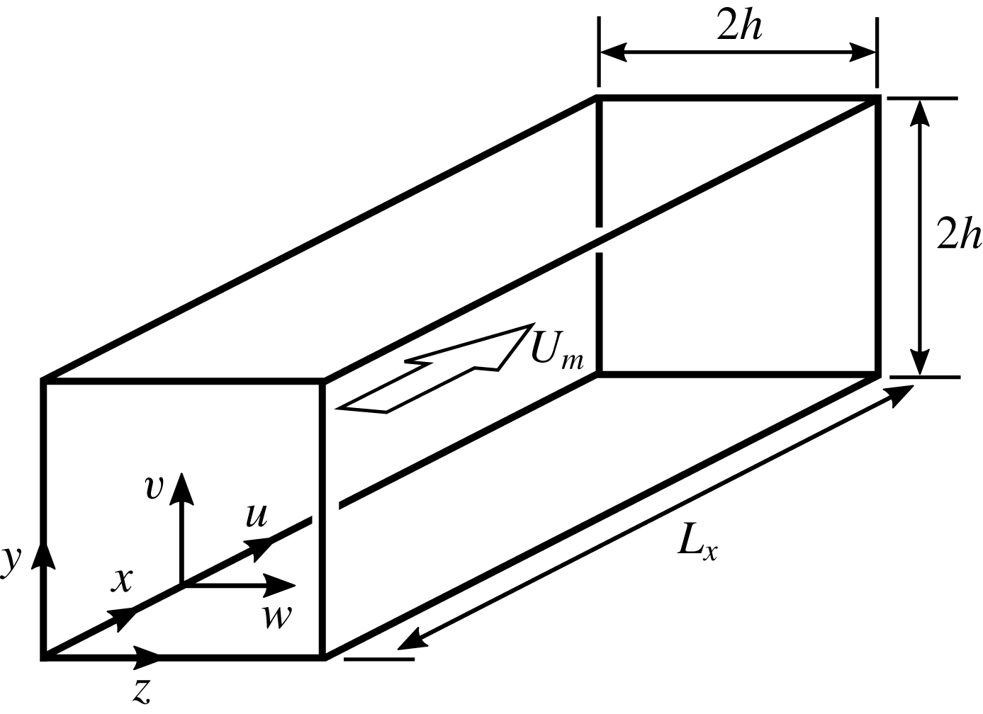
The turbulent flow data to be used are generated from the DNS of a constant-property fluid driven through a rectangular domain that is bounded by four equal, plane, smooth, and rigid walls and two opposing flow-through sides: see figure 1. The
 $x$
-axis is normal to the open boundaries, and along it a pressure gradient is applied that maintains the mean flow and ensuing turbulence, which are assumed to be fully developed. Instead of inflow and outflow conditions on the velocity at the open boundaries, the usual assumption of an instantaneously periodic velocity field is made. On the four walls, no-slip and impermeability conditions are applied. The dimensions of the domain in
 $x$
,
 $y$
and
 $z$
are
 $L_{x}$
,
 $2h$
and
 $2h$
, respectively.
Geometry and axes system.

The dynamical model for this flow is the Navier–Stokes equations constrained by the incompressibility of the fluid. Defining the alternate space coordinates
 $(x_{1},x_{2},x_{3})\equiv (x,y,z)$
and velocity components
 $(u_{1},u_{2},u_{3})\equiv (u,v,w)$
, the governing equations are
 $$\begin{eqnarray}\displaystyle \frac{\unicode[STIX]{x2202}u_{i}}{\unicode[STIX]{x2202}t}+\frac{1}{2}\left[u_{j}\frac{\unicode[STIX]{x2202}u_{i}}{\unicode[STIX]{x2202}x_{j}}+\frac{\unicode[STIX]{x2202}u_{i}u_{j}}{\unicode[STIX]{x2202}x_{j}}\right]=-\frac{\unicode[STIX]{x2202}p}{\unicode[STIX]{x2202}x_{i}}+\unicode[STIX]{x1D708}\frac{\unicode[STIX]{x2202}^{2}u_{i}}{\unicode[STIX]{x2202}x_{j}\unicode[STIX]{x2202}x_{j}}-\frac{\text{d}P}{\text{d}x}\unicode[STIX]{x1D6FF}_{i1} & & \displaystyle\end{eqnarray}$$
and
 $$\begin{eqnarray}\displaystyle \frac{\unicode[STIX]{x2202}u_{j}}{\unicode[STIX]{x2202}x_{j}}=0, & & \displaystyle\end{eqnarray}$$
where the summation convention over repeated subscripts applies with
 $t$
,
 $p$
and
 $\unicode[STIX]{x1D708}$
being the time, kinematic pressure and kinematic viscosity respectively;
 $\text{d}P/\text{d}x$
is the imposed streamwise pressure gradient, which at every instant is uniform throughout the fluid volume;
 $\unicode[STIX]{x1D6FF}_{i1}$
is the Kronecker function. The skew-symmetric form of the nonlinear terms shown in (2.1) is coded for its enhanced numerical stability.
The mean velocity components will be denoted by
 $U$
,
 $V$
and
 $W$
and the corresponding fluctuations by
 $u^{\prime }$
,
 $v^{\prime }$
and
 $w^{\prime }$
. The constant bulk flow velocity will be
 $U_{m}$
, mean centreline velocity
 $U_{c}$
, and the time-averaged value of
 $\text{d}P/\text{d}x$
is written
 $\overline{\text{d}P/\text{d}x}$
. The friction velocity
 $u_{\unicode[STIX]{x1D70F}}$
determined by
 $$\begin{eqnarray}\displaystyle u_{\unicode[STIX]{x1D70F}}^{2}=-\frac{h}{2}\overline{\frac{\text{d}P}{\text{d}x}} & & \displaystyle\end{eqnarray}$$
will be used as one velocity scale and in the definition
 $Re^{+}=hu_{\unicode[STIX]{x1D70F}}/\unicode[STIX]{x1D708}$
. The bulk Reynolds number is defined here by
 $Re_{m}=2hU_{m}/\unicode[STIX]{x1D708}$
. Flow data scaled with
 $u_{\unicode[STIX]{x1D70F}}$
and
 $\unicode[STIX]{x1D708}$
are referred to being in wall units/scales as it is common usage, although the suitability of such a descriptive term in the square duct flow is uncertain. A local friction velocity over the duct perimeter can be calculated from the normal derivative of the local wall-parallel velocity with values ranging between zero and about
 $1.1u_{\unicode[STIX]{x1D70F}}$
. It has a small off-
 $x$
component which averages to zero over the perimeter, while the
 $x$
component averages to
 $u_{\unicode[STIX]{x1D70F}}$
to at least three significant digits. Quantities in wall units will be marked with the plus symbol in the superscript position.
All dependent flow variables are expanded in finite Fourier sums along the homogeneous direction
 $x$
that are substituted into (2.1) and (2.2). The orthogonality of the Fourier basis is applied to derive a set of equations for the velocity amplitudes of every streamwise mode. The nonlinear products are evaluated in real space using
 $3/2$
longer vectors in the streamwise direction and are truncated back to their original length after they have been retransformed into Fourier space.
Spatial approximations in the transverse directions
 $y$
and
 $z$
of the equations for each Fourier mode are based on the spectral element method of Patera (Reference Patera1984). The cross-flow area is divided into conforming quadrilateral elements and within each one the velocity and pressure variables are expanded in Lagrange polynomials over the Gauss–Lobatto–Legendre (GLL) quadrature nodes of a chosen order. With this basis, the variational form of the momentum and continuity equations are discretized using the GLL quadrature over the same set of nodes for evaluating the projection integrals. Here, the order of polynomial expansion for the velocity and pressure variables is the same – usually referred to as the
 $\mathbb{P}_{N}-\mathbb{P}_{N}$
method, where
 $\mathbb{P}_{N}$
is the space of polynomials of degree
 $N$
– and therefore boundary conditions for the velocity and pressure fields are necessary. On the walls, the numerical boundary conditions for the velocity are no-slip and no-through flow. The time advancement scheme uses the two-step higher-order splitting method of Leriche et al. (Reference Leriche, Perchat, Labrosse and Deville2006). In the first step, the pressure Laplacian is inverted where the nonlinear source terms and wall-normal pressure gradients are extrapolated by a second-order in time scheme. In the second step, the viscous effects are advanced with an implicit second-order Euler scheme. The overall accuracy is second-order in time and it is free from (other than the constant) spurious pressure modes. The matrices that arise from the pressure and viscous elliptic operators and that are bounded by the rectangular cross-section of the duct are efficiently inverted by diagonalization (see Lynch, Rice & Thomas Reference Lynch, Rice and Thomas1964). The zero wavenumber component of the pressure equation is used to fix the global constant pressure mode by enforcing a zero mean pressure at one corner.
The flow is driven by an adjustable streamwise pressure gradient that maintains a prescribed flow rate to an accuracy better than eleven significant digits (Deschamps Reference Deschamps1988). A laminar flow profile used in the initial conditions is linearly stable, and therefore setting off transition to turbulence requires finite amplitude perturbations. A key stage in this transition process is found to be the formation of laminar streaks – elongated regions of positive and negative streamwise velocity perturbations – present over most of the cross-section and crucially near the walls. An efficient method for attaining such a state is choosing the initial conditions to be the sum of a laminar profile at a low Reynolds number onto which several vortex rings are added whose positions, extents, orientations and strengths are varied using a pseudo-random number generator. The velocity field of each ring is calculated by taking the
 $\text{curl}$
of a vector potential. The Cartesian velocity components of each ring are computed from
 $$\begin{eqnarray}\displaystyle \unicode[STIX]{x1D735}\times [A\exp (-a^{2}r^{2})\boldsymbol{e}_{R}], & & \displaystyle\end{eqnarray}$$
where
 $A$
is an amplitude parameter,
 $a^{-1}$
is a spatial scale,
 $r^{2}={r_{x}}^{2}+{r_{y}}^{2}+{r_{z}}^{2}$
the distance from the symmetry centre of the ring, and
 $\boldsymbol{e}_{R}$
a unit vector that defines the ring symmetry axis and thus its orientation. The composite initial field is filtered to remove sharp gradients and integrated forward in time for about five
 $h^{2}/\unicode[STIX]{x1D708}$
units to ensure that most of the initial vorticity has diffused to the walls. This phase is followed by successive increases of the Reynolds number with matching grid refinements until the final values of the parameters aimed at are reached. These are shown in table 1. With the final set of parameters, the simulations are advanced for a sufficiently long time until a steady mean state in the evolving global statistics is detected. A set of files containing the velocity and pressure fields at equally spaced time intervals is extracted from the later part of the steady-state segment of each simulation. During the time integration segment for storing field data, the incremental changes of the running global averages of the driving pressure gradient, turbulent kinetic energy and dissipation rate are monitored. When changes in these fall below 0.5 % over the most recent
 $3h/u_{\unicode[STIX]{x1D70F}}$
interval, runs are continued as needed with periodic testing of the updated velocity intensity profiles and secondary flows. The admissible type of convergence in the intensities for
 $Re^{+}=861$
can be seen in figure 9(a,b), where the marks are the results of averaging over the shorter interval
 $10.6h/u_{\unicode[STIX]{x1D70F}}$
. The intensities are well converged, especially along the diagonal. The more sensitive secondary flows, which depend on the integrated derivatives of the transverse Reynolds stresses in (6.1), are shown in figure 7(b). The secondary flow peak magnitude near the corner has converged well, while the outer flow nearer the duct centre where the secondary velocity maximum magnitude is
 ${\sim}0.013U_{c}$
has decreased by less than 3 % with
 $6h/u_{\unicode[STIX]{x1D70F}}$
or over
 $50\,\%$
of additional averaging. The difficulty of converging on the mean secondary flows is due to their unusual shape and relatively low magnitude; they are the outcome of averaging typical quasi-circular instantaneous vortices. This weak part of the mean flow field understates the effects of the corner on the turbulent flow which are more pronounced in other statistics such as the turbulent kinetic energy shown in figure 10. The distinctive two-minima structure is also found in separate simulations: here, when
 $Re^{+}=605$
and in Zhang et al. (Reference Zhang, Trias, Gorobets, Tang and Oliva2015) (figure 7
b,c). The statistics computed from each database use time and all available geometrical symmetries – when applicable – and the use is denoted with an overbar over the relevant fluctuating variables.
Physical and numerical characteristics of the present simulations.
 $U_{c}$
is the mean centreline velocity. The entries between parentheses are domain sizes of additional simulations for the same Reynolds numbers using an appropriately reduced number of Fourier modes.
 $N$
is the degree of the Lagrange polynomial within each element.
 $N_{x}$
is the number of Fourier modes in
 $x$
;
 $N_{y}$
is the number of independent GLL nodes in
 $y$
; the number of independent nodes in
 $z$
is equal to
 $N_{y}$
. The minimum
 $\unicode[STIX]{x0394}y^{+}$
is the normal node spacing closest to the boundaries. The cross-flow node spacing
 $\unicode[STIX]{x0394}z^{+}$
has an identical distribution to
 $\unicode[STIX]{x0394}y^{+}$
. Database time spans are in
 $h/u_{\unicode[STIX]{x1D70F}}$
units.

The characteristics of the simulations that are presented here are chosen around a set of constraints of acceptable node spacings. One additional limit is cited in Karniadakis & Sherwin (Reference Karniadakis and Sherwin1999, p. 283). It is that there should be least ten cosine nodes within nine wall units from each boundary in the wall-normal direction. The least compliant simulations in this respect use nine GLL nodes below the nominal nine wall units and the experience here is that polynomial order and the wall-parallel resolution must also be considered. The elements in the cross-section are generally laid out according to a hyperbolic tangent distribution and are mildly stretched so they cluster near the boundaries, but occasionally the common size of the wall-touching elements is chosen separately. The element sizes, their distribution and the polynomial order are selected for minimizing occasional reflections in the instantaneous dissipation rate peaks when they happen to straddle interelement boundaries.
In terms of the Kolmogorov length
 $\unicode[STIX]{x1D702}=(\unicode[STIX]{x1D708}^{3}/\unicode[STIX]{x1D716}_{v})^{1/4}$
, where
 $\unicode[STIX]{x1D716}_{v}$
is the volume-averaged mean dissipation rate – see definitions in § 3 below – the maximum cross-flow grid spacing is
 $3\unicode[STIX]{x1D702}$
and the streamwise spacing is about
 $5\unicode[STIX]{x1D702}$
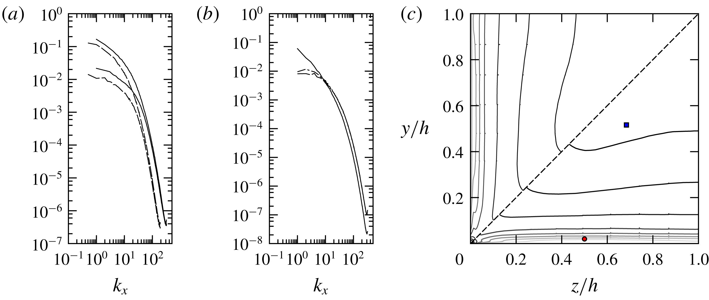
. The turbulent velocity spectra for the two highest Reynolds numbers in figure 2(a,b) have upturns near the cutoff wavenumbers, indicating insufficient viscous dissipation. The dissipation rate contours of figure 2(c) have small upticks on the inter-element boundaries – derivatives are calculated in the strong form – but only on those boundaries normal to the nearest wall and not those parallel to it. Taken together, the three figures suggest that intermittent steep wall-parallel gradients may require finer node spacing. The difference between the volume and sample averaged input power and the similarly averaged sum of the turbulent and mean-field dissipation rates is less than 3 %.
There is a stability restriction on the time step owing to the explicit temporal extrapolation of the nonlinear terms. Numerical experiments are conducted to establish time step limits for each Reynolds number and spatial resolution. For a fixed distribution of elements, the time step limit scales close to
 $1/N^{2}$
, but the eventual choice has to allow a safety margin, making it smaller than these estimates, otherwise occasionally very high velocity events can at some point destabilize the computations.
(a) Streamwise spectra of
 $u^{\prime }$
(top set) and
 $v^{\prime }$
(wall-normal, lower set) velocity components at a point near the overall maximum of the dissipation rate
 $\unicode[STIX]{x1D716}$
:
 $(y,z)\simeq (0.02h,0.5h)$
; ——,
 $Re^{+}=861$
; — —,
 $Re^{+}=605$
. (b) Streamwise velocity spectra for
 $Re^{+}=861$
at
 $(y,z)=(0.516h,0.684h)$
; ——,
 $u^{\prime }$
; —– —–,
 $v^{\prime }$
; — ⋅ —,
 $w^{\prime }$
. (c) Contours of the dissipation rate
 $\unicode[STIX]{x1D716}^{+}$
. Above the corner bisector:
 $Re^{+}=605$
; below the bisector:
 $Re^{+}=861$
. The round point marks the location of the spectra in (a); the square point marks spectra in (b).

The nonlinear products are evaluated in physical space at the GLL nodes and extended Fourier grid which ensures dealiased results for the homogeneous direction modes only. For
 $Re^{+}>350$
(approximately), the simulations may show a slow build-up of energy at the highest and nearby wavenumbers over a continually broadening interval. With high-order polynomials, simulations can be sustained for tens of thousands of time steps, but they would be increasingly tainted by the unphysical energy accumulation at high wavenumbers. A space–time filtering method based on the two-grid polynomial interpolation of Fischer & Mullen (Reference Fischer and Mullen2001) is used. Every 17 time steps, the three velocity components are interpolated onto the GLL grid for polynomial expansion one less than the simulation and then they are interpolated back onto the original grid. The
 $C^{0}$
continuity of the velocity field at the interelement boundaries is preserved by this procedure. The weighted averages of the original and filtered fields are used to make one first-order implicit Euler step and then proceed with the second-order scheme. The leading error term of the backward Euler step is diffusive. The filter-Euler step would normally affect the overall time-accuracy of the simulations, but the relatively infrequent use of filtering and the cautious choice of the time step mitigate this effect. Both filtering frequency and averaging weights have been chosen to minimize the energy accumulating near the high wavenumber end of the velocity spectra: see figure 2(a,b).
The simulations are run on a dedicated computer system built around a single socket motherboard (Intel LGA2011, X79 chipset.) The central processor (CPU) is the six-core Intel I7 3930K running at stock speeds – base and turbo – but the bulk of the computational work is carried on two Graphics Processing Units (GPUs) that are used as double-precision floating-point coprocessors. The GPUs, two AMD Radeon R9 280X, are mounted on two 16 lane PCI Express 3.0 (PCIe) slots with the hardware lanes built into the processor, 40, enabling the maximum data transfer rate allowed by this communication interface for both GPUs. Parallelization on the CPU side of the code is built around the OpenMP libraries and is used for launching multiple threads either for doing calculations or controlling data transfers and computing activities associated with each GPU. The code executing on the GPUs, a collection of routines called kernels, conforms to the OpenCL 1.2 standard. The evaluation of the (skew-symmetric) nonlinear terms, Fourier transforms and the sequence of matrix operations needed for finding the pressure and velocity fields are divided among the GPUs, whereas all computations that involve direct stiffness or engage data from the previous two time steps are multithreaded on the CPU. Every simulation is preceded by an optimization and code-checking phase. For the
 $Re^{+}=605$
simulation with 132 million nodes, the averaged elapsed time for one time step is
 $0.085~\unicode[STIX]{x03BC}\text{s}$
per grid point with GPU occupancy averaging 41 %, which includes data transfer times over the PCIe interface; the matrix–matrix multiplication GPU kernels in the pressure and velocity calculations, which implement a tiled product algorithm and are batched in groups of 64 wavenumbers, are executing at the sustained rate of
 $430\times 10^{9}$
double precision floating point operations per second per GPU. The figures corresponding to 213 million points of
 $Re^{+}=861$
are
 $0.1~\unicode[STIX]{x03BC}\text{s}$
, 53 % and
 $490\times 10^{9}$
floating point operations per second per GPU, respectively.
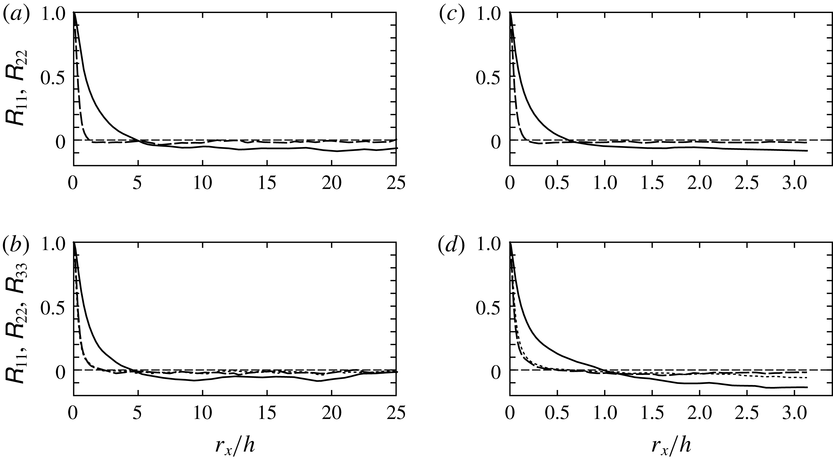
Two-point velocity correlation coefficients for two Reynolds numbers: (a,b)
 $Re^{+}=157$
; (c,d)
 $Re^{+}=861$
. Figures (a) and (c) are for nodes closest to
 $y=z=0.2h$
on the diagonal. Figures (b) and (d) are nearest to
 $(y,z)=(0.12h,0.995h)$
. For points on the diagonal, the two cross-flow coefficients are identical due to symmetry: ——,
 $\unicode[STIX]{x1D619}_{11}$
; — — —,
 $\unicode[STIX]{x1D619}_{22}$
; - - -,
 $\unicode[STIX]{x1D619}_{33}$
.

2.2 Two-point correlations
One largely overlooked aspect of duct turbulence surfaced in the precursor simulations in Gavrilakis (Reference Gavrilakis1992). It was the slow decay of the two-point streamwise velocity correlations in the homogeneous direction as
 $L_{x}$
was increased, which was not evident in the final computation with
 $L_{x}=20\unicode[STIX]{x03C0}h$
. Some subsequent simulations – Huser & Biringen (Reference Huser and Biringen1993), Sharma (Reference Sharma2004), Fang et al. (Reference Fang, Yang, Wang and Bergstrom2017) – have also encountered persistent correlations of
 $u^{\prime }$
. But the rationale for the ‘abnormal extent’ of the space correlations in the
 $u^{\prime }$
field of commonly occurring flows given by Townsend (Reference Townsend1976, p. 111 and §§ 7.20–7.21), could be relevant to duct turbulence. Generalizing, Townsend suggested that fluctuations induced by wall-stress variations ‘whatever the cause’ may persist through the whole flow.
The two-point longitudinal velocity correlation coefficients are defined by
 $$\begin{eqnarray}\displaystyle \unicode[STIX]{x1D619}_{ij}(r_{x},y,z)=\frac{\overline{u_{i}^{\prime }(x,y,z)u_{j}^{\prime }(x+r_{x},y,z)}}{\sqrt{\overline{[u_{i}^{\prime }(y,z)]^{2}}\;\;\overline{[u_{j}^{\prime }(y,z)]^{2}}}}, & & \displaystyle\end{eqnarray}$$
where
 $r_{x}$
is now the streamwise separation. In figure 3, the three diagonal components are shown for two transverse locations and for the highest and lowest Reynolds numbers available here. The
 $Re^{+}=157$
results with the longer
 $L_{x}$
of
 $16\unicode[STIX]{x03C0}h$
show that
 $\unicode[STIX]{x1D619}_{11}$
remains close to
 $-$
7 % near the maximum separation for points on the diagonal (figure 3
a), which supports the use of
 $L_{x}=20\unicode[STIX]{x03C0}h$
in the earlier simulation employing a comparably low Reynolds number. Persistence in
 $\unicode[STIX]{x1D619}_{11}$
is found over a substantial fraction of the duct cross-section as well as a decline toward zero in other parts as in figure 3(b). Tests with shorter domains (table 1) show some effects for
 $Re^{+}$
below 300, but no such effects are detectable above the statistical uncertainty for
 $Re^{+}=605$
. These can be understood, and perhaps predicted, by referring to the structure of the
 $u^{\prime }$
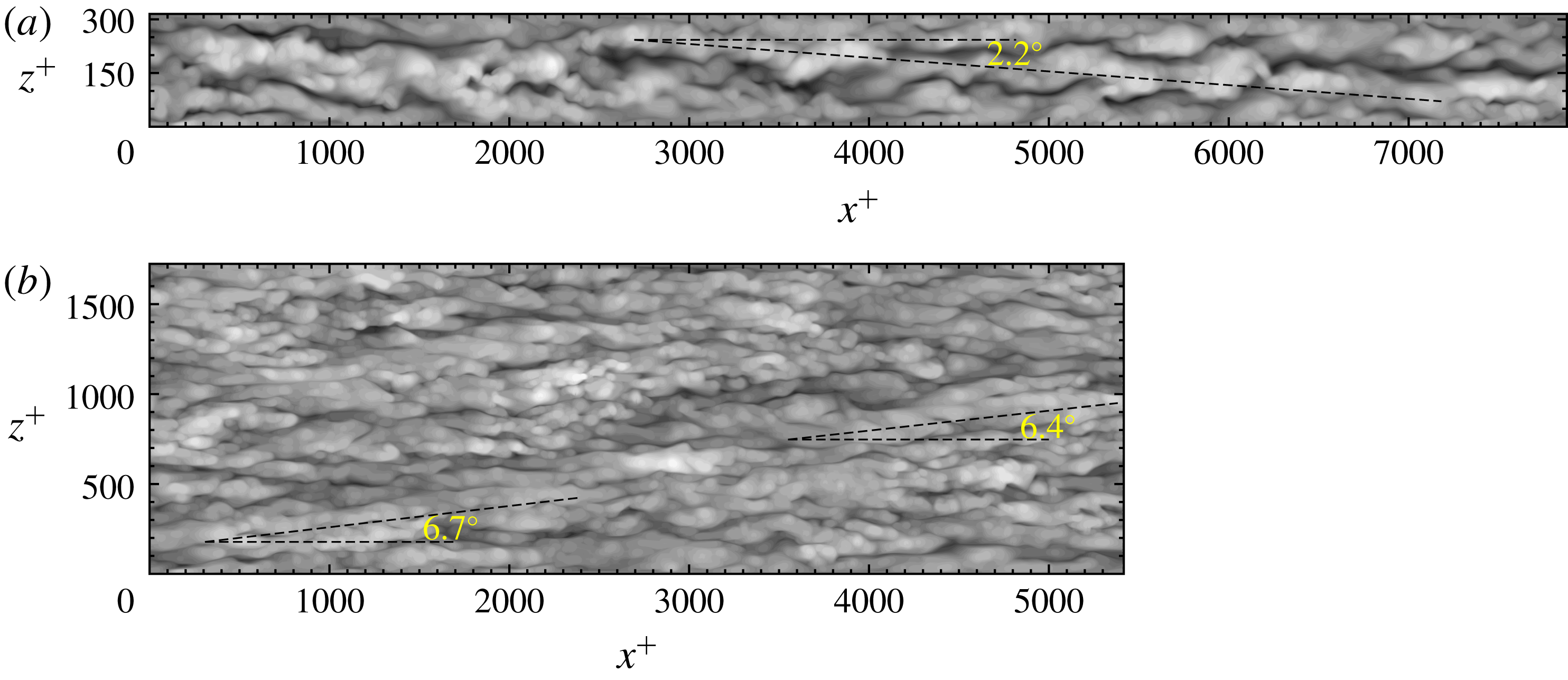
component in the instantaneous wall turbulence. At the lowest Reynolds number, the
 $u^{\prime }$
distribution near the walls is dominated by a single pair of long high- and low-speed streaks (figure 4
a), from which the effects of a shorter domain may be inferred. Even though the mechanism is nonlinear, reducing
 $L_{x}$
will tend to hinder the lateral displacement of the streaks, thus heightening alignment with the
 $x$
-axis and therefore increasing
 $r_{x}$
to the first zero crossing of
 $\unicode[STIX]{x1D619}_{11}$
, whereas the intensity of
 $u^{\prime }$
near the wall will appear to increase or decrease depending on the length of the cut domain and position in the cross-section. These effects are petering out beyond
 $Re^{+}=295$
and figure 4(b) shows why this occurs: a gradual build-up of a substantial sub-
 $2h$
turbulent component. For example, the
 $Re^{+}=605$
simulations with
 $L_{x}=4\unicode[STIX]{x03C0}h$
and
 $2\unicode[STIX]{x03C0}h$
show a difference in the peak values of
 $\overline{{u^{\prime }}^{2}}/u_{\unicode[STIX]{x1D70F}}^{2}$
on the wall bisector of about 1 %; assuming that such a trend would continue, a smaller effect would be expected when
 $Re^{+}=861$
. Overall, for the simulations of table 1 and the statistics used herein, no
 $L_{x}$
effects are detectable above the sampling uncertainty, and therefore all simulations including the
 $Re^{+}=861$
(figure 3
c,d) are considered reliable approximations to the decorrelated cases.
Instantaneous turbulent velocity field component
 ${u^{\prime }}^{+}$
over a plane near one of the four walls. (a)
 $Re^{+}=157$
at
 $y^{+}=16.3$
. The
 $z$
-axis has been expanded by a factor of 2. Velocity data span the interval
 $[-11.7,10.8]$
. Greyscale limits: black, minimum; white, maximum. The dashed line traces a high-speed region; it is at an angle of
 $2.2^{\circ }$
to the
 $x$
-axis. (b)
 $Re^{+}=861$
at
 $y^{+}=22.6$
. True aspect ratio. Velocity range
 $[-8.3,8.2]$
.

We must still account for
 $\unicode[STIX]{x1D619}_{11}$
being negative at larger separations, which is also found in Huser & Biringen (Reference Huser and Biringen1993) and Sharma (Reference Sharma2004). Figure 4(a) appears helpful at illustrating the flow underlying a long wavelength oscillatory correlation. High- and low-speed regions are seen extending from wall to wall and exceeding
 $L_{x}/2$
in downstream length, but at a small angle to the
 $x$
-axis. The data of figure 4(a) show a streak angle with the
 $x$
-axis of
 $2.2^{\circ }$
, and therefore the lateral displacement of the high-speed pattern over the duct half-length will be
 $z^{+}\sim 150$
. Since the typical separation of adjacent high- and low-speed streaks in boundary layers and plane channels is known to be about 50 wall units, a pair of points aligned on the
 $x$
-axis are more likely to fall on opposite-signed streaks at (near) maximum
 $r_{x}$
. For
 $\unicode[STIX]{x1D619}_{11}$
to remain wholly negative beyond the first zero crossing (figure 3
a), a shallower structure angle must be prevalent at that position. It has been assumed that the streak lateral separation scaling holds for ducts as well and all simulations shown here appear to have this streak spacing. Similarly, the
 $u^{\prime }$
distribution for
 $Re^{+}=861$
over planes parallel to the walls (figure 4
b) now has oblique sequences of structures stretching over distances comparable to the duct’s half-length. The angles with the
 $x$
-axis could be as high as
 $7^{\circ }$
, but for the instance shown, they are in the opposite sense to that in figure 4(a).
3 Friction factor
The Darcy–Weisbach friction factor
 $f$
for the fully developed straight square duct may be written as
 $f=8u_{\unicode[STIX]{x1D70F}}^{2}/U_{m}^{2}$
. For the fully developed laminar duct flow, an analytical expression for
 $f$
can be found from the solution of the streamwise momentum equation. The
 $U(y,z)$
profile is obtained in the form of an infinite sum, which can be integrated over the cross-section to arrive at a related infinite sum for the mean flow velocity
 $U_{m}$
(Timoshenko & Goodier Reference Timoshenko and Goodier1951, pp. 275–278). The sum of the first fifty terms of this series leads to
 $$\begin{eqnarray}\displaystyle f=\frac{56.9028}{Re_{m}}. & & \displaystyle\end{eqnarray}$$
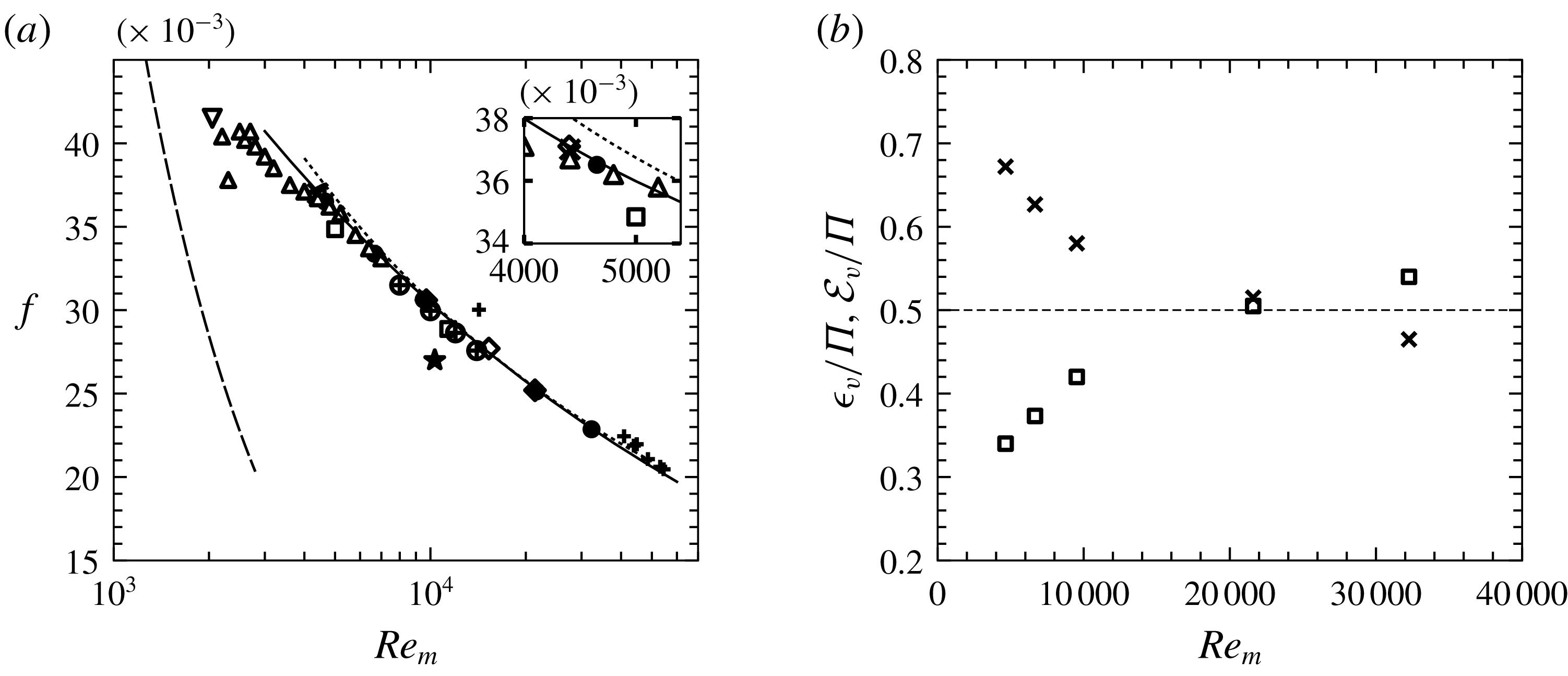
The curve for this expression together with turbulent flow data from a number of published sources are shown in figure 5(a). The two recent simulation datasets, that of Zhang et al. (Reference Zhang, Trias, Gorobets, Tang and Oliva2015) and the present one, are in good agreement over the range of Reynolds numbers shown. The experimental correlation for circular pipe turbulence in McKeon et al. (Reference McKeon, Swanson, Zagarola, Donnelly and Smits2004) shows consistently slightly higher values than the duct simulations, but the observed differences are less than the uncertainties in the data. This comparison is based on the equality of the Reynolds numbers of ducts and pipes, which may be meaningfully realized when the same volume flow rate is driven through devices that have identical perimeter lengths. This corresponds to the square duct’s side length being
 $\unicode[STIX]{x03C0}/4$
times smaller than the pipe’s diameter. The present simulation data fit the power law
 $$\begin{eqnarray}\displaystyle f=0.281Re_{m}^{-1/4.13}, & & \displaystyle\end{eqnarray}$$
with the maximum absolute difference between the simulation friction factors and this approximate relation of 0.5 %. Note that the difference between the stress from the mean pressure drop and the perimeter-integrated stress derived from the
 $U(y,z)$
profile is 0.1 % for the
 $Re^{+}=605$
simulation, but below 0.05 % for the remaining Reynolds numbers.
(a) Darcy–Weisbach friction factor for the square duct as a function of
 $Re_{m}$
: – – –, fully developed laminar flow equation (3.1);
 $\cdots \cdots$
, turbulent pipe flow correlation adaptation by McKeon et al. (Reference McKeon, Swanson, Zagarola, Donnelly and Smits2004); ——,
 $f=0.281Re_{m}^{-1/4.13}$
, power law fit of current simulation data; ▫, Marin et al. (Reference Marin, Vinuesa, Obabko and Schlatter2016); ♢, Zhang et al. (Reference Zhang, Trias, Gorobets, Tang and Oliva2015);
 $\star$
, Huser & Biringen (Reference Huser and Biringen1993),
 $Re^{+}=300$
; ▵, Pinelli et al. (Reference Pinelli, Uhlmann, Sekimoto and Kawahara2010) and Uhlmann et al. (Reference Uhlmann, Pinelli, Kawahara and Sekimoto2007); ▿, Biau, Soueid & Bottaro (Reference Biau, Soueid and Bottaro2008),
 $Re^{+}=75$
;
 $\times$
, Gavrilakis (Reference Gavrilakis1992),
 $Re^{+}=150$
(just discernible in the inset);
 $\oplus$
, Sakai (Reference Sakai2016);
 $+$
, Owolabi, Dennis & Poole (Reference Owolabi, Dennis and Poole2017); ●, present DNS results. The inset shows an expanded view of the points clustered near
 $Re^{+}=150$
. (b) Volume- and time-averaged dissipation rates as fractions of the average input power of the simulations shown in table 1. ▫, turbulent field;
 $\times$
, mean field.

The recently published set of experimental friction factors by Owolabi et al. (Reference Owolabi, Dennis and Poole2017) are closing in on the duct correlation near the higher Reynolds number end, but straying off from the consensus values toward the lower end. The scatter in the data of Uhlmann et al. (Reference Uhlmann, Pinelli, Kawahara and Sekimoto2007) and Pinelli et al. (Reference Pinelli, Uhlmann, Sekimoto and Kawahara2010) below
 $Re_{m}=4000$
is attributed by the authors to the ‘meta-stable’ state of the flow in this transitional Reynolds number range (M. Uhlmann, 2017, private communication.) The four data points taken from the thesis of Sakai (Reference Sakai2016) are consistently less than the data fit equation (3.2).
The mean power supplied to every simulation can be calculated from the last term of the time-averaged form of (2.1) for
 $i=1$
when it is multiplied through by
 $u$
and averaged over volume and time. The driving gradient is constant over the flow volume but not in time, whereas the volume flow rate
 $4h^{2}U_{m}$
is constant with
 $x$
and
 $t$
. These are used to derive the sample-mean power per unit mass,
 $\unicode[STIX]{x1D6F1}$
, maintaining the flow which is
 $$\begin{eqnarray}\displaystyle \unicode[STIX]{x1D6F1}=-U_{m}\overline{\frac{\text{d}P}{\text{d}x}}. & & \displaystyle\end{eqnarray}$$
For steady state conditions, the mean power input must equal the mean viscous dissipation rate. Letting
 $\unicode[STIX]{x1D61A}_{ij}=(\unicode[STIX]{x2202}U_{i}/\unicode[STIX]{x2202}x_{j}+\unicode[STIX]{x2202}U_{j}/\unicode[STIX]{x2202}x_{i})/2$
and
 $\unicode[STIX]{x1D634}_{ij}^{\prime }=(\unicode[STIX]{x2202}u_{i}^{\prime }/\unicode[STIX]{x2202}x_{j}+\unicode[STIX]{x2202}u_{j}^{\prime }/\unicode[STIX]{x2202}x_{i})/2$
be the mean and fluctuating strain rates, respectively, the dissipation rates for the mean and turbulent fields are
 $$\begin{eqnarray}\displaystyle {\mathcal{E}}=2\unicode[STIX]{x1D708}\unicode[STIX]{x1D61A}_{ij}\unicode[STIX]{x1D61A}_{ji}\quad \text{and}\quad \unicode[STIX]{x1D716}=2\unicode[STIX]{x1D708}\overline{\unicode[STIX]{x1D634}_{ij}^{\prime }\unicode[STIX]{x1D634}_{ji}^{\prime }}. & & \displaystyle\end{eqnarray}$$
Note that throughout this report, all derivatives in the statistics are computed in their strong form.
For a stationary flow within a domain of volume
 $V$
, the time- and volume-averaged dissipation rates of the mean (
 ${\mathcal{E}}_{v}$
) and turbulent (
 $\unicode[STIX]{x1D716}_{v}$
) fields add up to
 $\unicode[STIX]{x1D6F1}$
or
 $$\begin{eqnarray}\displaystyle \unicode[STIX]{x1D6F1}=\frac{1}{V}\int _{V}{\mathcal{E}}\,\text{d}V+\frac{1}{V}\int _{V}\unicode[STIX]{x1D716}\,\text{d}V\equiv {\mathcal{E}}_{v}+\unicode[STIX]{x1D716}_{v}. & & \displaystyle\end{eqnarray}$$
This allows us to rewrite the friction factor in terms of the mean-field and turbulent contributions. From definition (2.3) and equations (3.3) and (3.5), the form of
 $f$
can be recast into
 $$\begin{eqnarray}\displaystyle f=4h\frac{\unicode[STIX]{x1D6F1}}{U_{m}^{3}}=4h\frac{{\mathcal{E}}_{v}+\unicode[STIX]{x1D716}_{v}}{U_{m}^{3}}, & & \displaystyle\end{eqnarray}$$
where
 $4h$
is half the perimeter length. This expression for
 $f$
allows the calculation of the relative contribution of turbulence to the observed drag, but the two terms are not independent because turbulence modifies the mean-field gradients, which are factors in determining both
 ${\mathcal{E}}_{v}$
and turbulence generation itself. The nonlinear mechanism in the duct settles on the partition shown in figure 5(b). At the lowest
 $Re_{m}$
, it emerges that the turbulent part is just over one-third of the total, which is not insubstantial since the Reynolds number is relatively close to the value at which the flow will revert to the laminar state. The cross-over point between the two terms occurs near
 $Re^{+}=605$
, which is probably a significant threshold for turbulent flows in this geometry. Beyond this, the rate with which the two sets of dissipation statistics recede appears quite low.
4 The velocity field
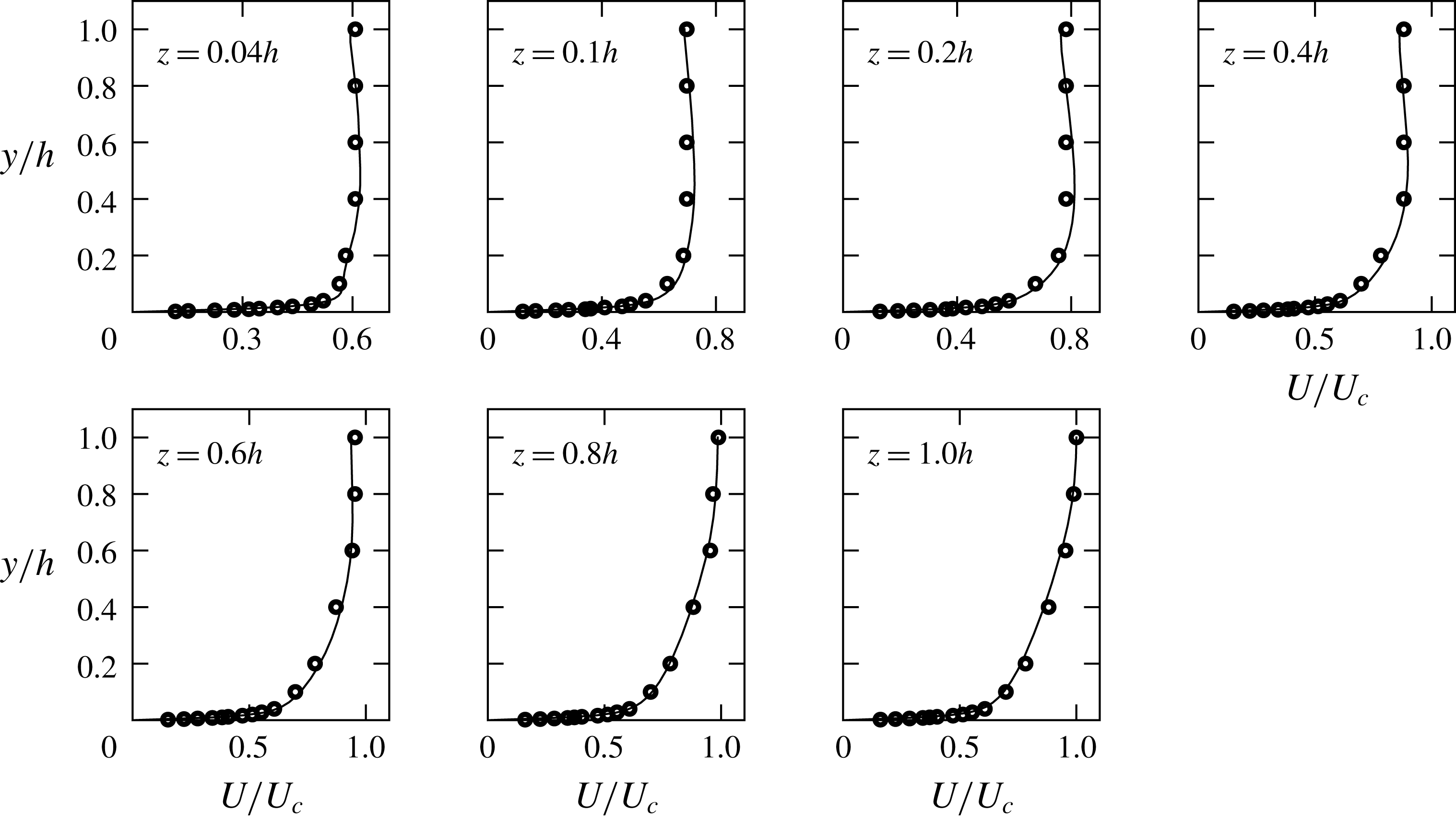
In figure 6, sections of the
 $U(y,z)$
field measured by Hoagland (Reference Hoagland1960) for
 $Re_{m}=34\,300$
are compared with data from the nearest stations of the
 $Re^{+}=861$
(
 $Re_{m}=32\,258$
) simulation. The
 $Re_{m}$
of the two flows differ by less than 7 % and there are small systematic differences between the sampled mean fields. For
 $y,z<0.7h$
, the simulation data show slightly higher values whereas near the wall bisectors, the differences appear reversed which, if the measurements were taken ‘as is’, would be consistent with weaker secondary flows for the experiment and a relatively lower turbulence level. However, increasing
 $Re_{m}$
tends to flatten the mean profile as the trend in
 $U_{c}/U_{m}$
in table 1 attests. Likely explanations for these rather small differences include uncertainties linked to the measuring procedure and lack of full development in the flow.
Mean streamwise velocity profiles along transverse lines normal to the
 $z$
-axis. Open symbols are the measurements of Hoagland (Reference Hoagland1960) for
 $Re_{m}=34\,300$
. The continuous lines are from the nearest stations of the current
 $Re_{m}=32\,258$
(
 $Re^{+}=861$
) simulation. The scaling velocity is the centreline value
 $U_{c}$
of each dataset.

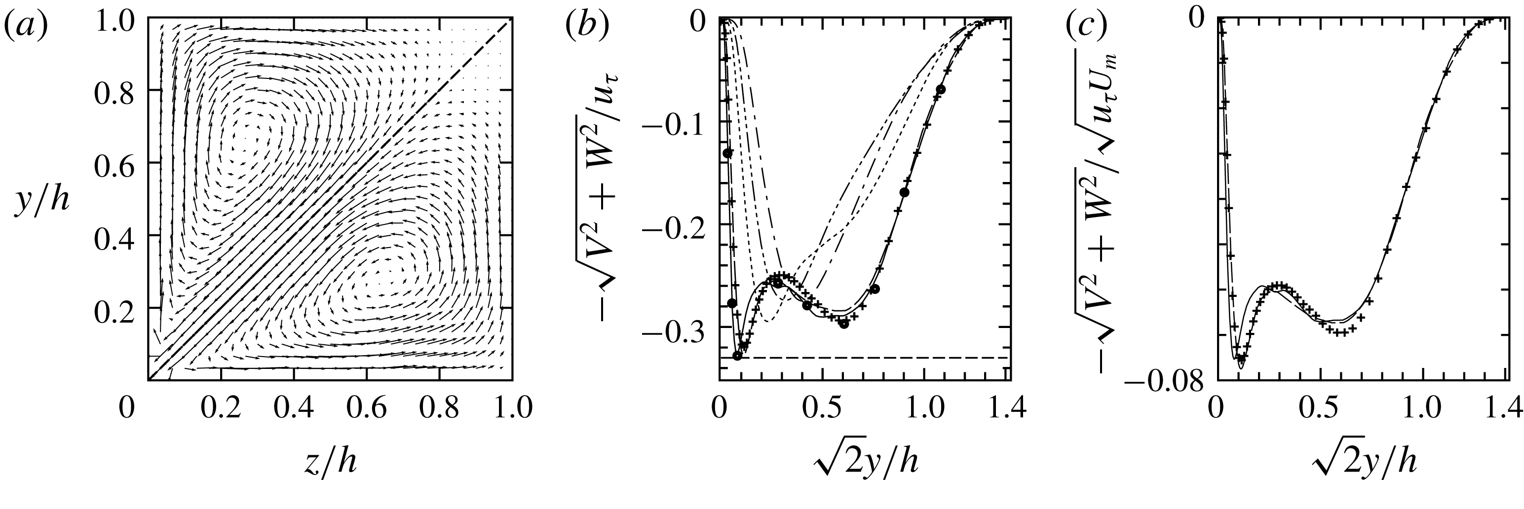
(a) Mean secondary flows in an octant. The velocity components have been interpolated onto a uniform grid from the GLL nodes of each simulation. Vectors above the diagonal are from the
 $Re^{+}=605$
simulation; those below are from
 $Re^{+}=861$
. (b) Signed velocity magnitude in wall units along a diagonal half: ——,
 $Re^{+}=861$
; — — —,
 $Re^{+}=605$
;
 $\cdots \cdots$
,
 $Re^{+}=295$
; —
 $\cdots \,$
—,
 $Re^{+}=215$
; — ⋅ —,
 $Re^{+}=157$
;
 $+$
, Zhang et al. (Reference Zhang, Trias, Gorobets, Tang and Oliva2015)
 $Re^{+}=600$
. The round markers are from the
 $Re^{+}=861$
simulation, but with a reduced averaging span of
 $10.6h/u_{\unicode[STIX]{x1D70F}}$
. The level of the horizontal dashed line is
 $-0.33$
. (c) Signed velocity magnitude along the half-diagonal with mixed scaling: ——,
 $Re^{+}=861$
; — — —,
 $Re^{+}=605$
;
 $+$
, Zhang et al. (Reference Zhang, Trias, Gorobets, Tang and Oliva2015),
 $Re^{+}=600$
.

One notable phenomenon of the turbulent duct flow is shown in figure 7(a). The secondary flow vector fields of the two highest Reynolds numbers appear quite similar. Their velocities on the diagonal are relatively close in magnitude and profile (figure 7
b,c), which are the preconditions, and are probably close to sufficient conditions for their similarity elsewhere. Each of the
 $Re^{+}=861$
and
 $Re^{+}=605$
curves has two (unsigned) maxima with the spacing between each curve’s two peaks widening with increasing Reynolds number; this trend evidently has a limit and suggests that the characteristics of the flow field are still evolving. A nascent secondary maximum is seen in the
 $Re^{+}=295$
curve. A number of trends are also evident for all but the lowest
 $Re^{+}$
. With increasing Reynolds number, the maximum velocity on the diagonal appears to approach
 $0.33u_{\unicode[STIX]{x1D70F}}$
, noting also that the maximum secondary velocity anywhere in the cross-section is just under
 $0.02U_{m}$
, which occurs off the diagonal and close to the corner near the turning of the secondary flow vectors. The positions of the maxima of the four highest
 $Re^{+}$
are within
 $\pm 2$
% of
 $y^{+}=z^{+}=48.8$
and it is below
 $\pm 0.1$
% for the two highest Reynolds numbers. The viscosity in this scaling compensates for the thinning of the viscous wall layers, but it is more difficult to discern how the global scale
 $u_{\unicode[STIX]{x1D70F}}$
enters in this since the local values of the wall stress plunge toward zero at the corner. A likely path would be through the determination of the base profile of
 $U$
, which drives the secondary flow generation instability. The outer velocity peaks for the two highest Reynolds numbers are related to the larger and most evident part of the flow in figure 7(a), and they are more accessible to measurement. Unlike their near-corner counterparts, they are evolving rapidly with changing Reynolds numbers and they are driven by turbulent vorticity processes (see below.) The data of Zhang et al. (Reference Zhang, Trias, Gorobets, Tang and Oliva2015) for
 $Re^{+}=600$
are included for comparison. The peak magnitude near the corner and its position on the diagonal agree well with the present
 $Re^{+}=605$
simulation. They also agree well on the position of the second maximum, but the Zhang et al. (Reference Zhang, Trias, Gorobets, Tang and Oliva2015) velocities are somewhat higher. The velocity values involved are relatively small and may still be subject to slow statistical convergence, but their agreement on the double structure of the secondary flow cells is unlikely to be coincidental. The broader outer peaks for the two highest
 $Re$
, which are about
 $0.6h$
from the nearest corner, scale with neither
 $u_{\unicode[STIX]{x1D70F}}$
(figure 7
b) nor
 $U_{m}$
(not shown), but when measured in units of
 $\sqrt{u_{\unicode[STIX]{x1D70F}}U_{m}}$
their peak and nearby values differ by less than 1 % (figure 7
c). However, by considering a small increase in
 $Re$
,
 ${\sim}15\,\%$
, above
 $Re^{+}=861$
it would appear that the persistence of this scaling is uncertain. Such an increase in
 $Re$
will create steeper gradients closer to the corner which entail displacing and strengthening of the outer secondary velocities. The formation of a tertiary peak nearer the duct centre at some nearby
 $Re$
will also become possible, in which case the generally assumed unitary character of secondary flows will have to be reconsidered.
The composite structure of the secondary flow presents modelling difficulties. Reynolds stress models (RANS) are good at capturing the bulk flow turbulent statistics and, quite likely, are going to struggle to predict the deep-corner profiles. But the transverse velocity scaling given above might be of help. Using rounded values, the simulations suggest augmenting the equations of motion of RANS computations with
 $|V^{+}|=|W^{+}|=1/3\sqrt{2}$
at four points (assuming full duct calculation) on the diagonals which are at
 $y^{+}=z^{+}\approx 50$
from the nearest duct walls. With these additional constraints, the system of equations is overdetermined and in most cases it will have no solution. One way for restoring system solvability in RANS computations is to discard boundary conditions for
 $V$
and
 $W$
at four points – perhaps the four corners. This amounts to allowing inflow or outflow at these four points to be determined by the algorithm. Ideally, these should turn out to be zero, but relatively small values would probably be tolerable. Significantly, this approach does away with having to shape turbulence models into producing the fragmented source of secondary flows, one part of which is a mean flow instability. But still, some information on the turbulent field must be supplied near the corner boundaries – typically the turbulent kinetic energy
 $k=(\overline{{u^{\prime }}^{2}}+\overline{{v^{\prime }}^{2}}+\overline{{w^{\prime }}^{2}})/2$
and
 $\unicode[STIX]{x1D716}$
– although now these are to be relied on for producing diffusion effects rather than driving the secondary flows. However, neither quantity scales in wall units; in figure 9(b), the apparent scaling of
 $\overline{{u^{\prime }}^{2}}$
with
 $u_{\unicode[STIX]{x1D70F}}^{2}$
is likely a transient phenomenon because the other two components do not scale, and therefore neither do
 $k$
and
 $\unicode[STIX]{x1D716}$
(figure 2
c). The lack of scaling in the cross-flow intensities is probably due to the diverse origins of the near-corner transverse fluctuations. One part would have propagated from distant pressure sources, another would be due to random incursions of the outer flow into the corner, but there is also a strong locally generated component whose description follows.
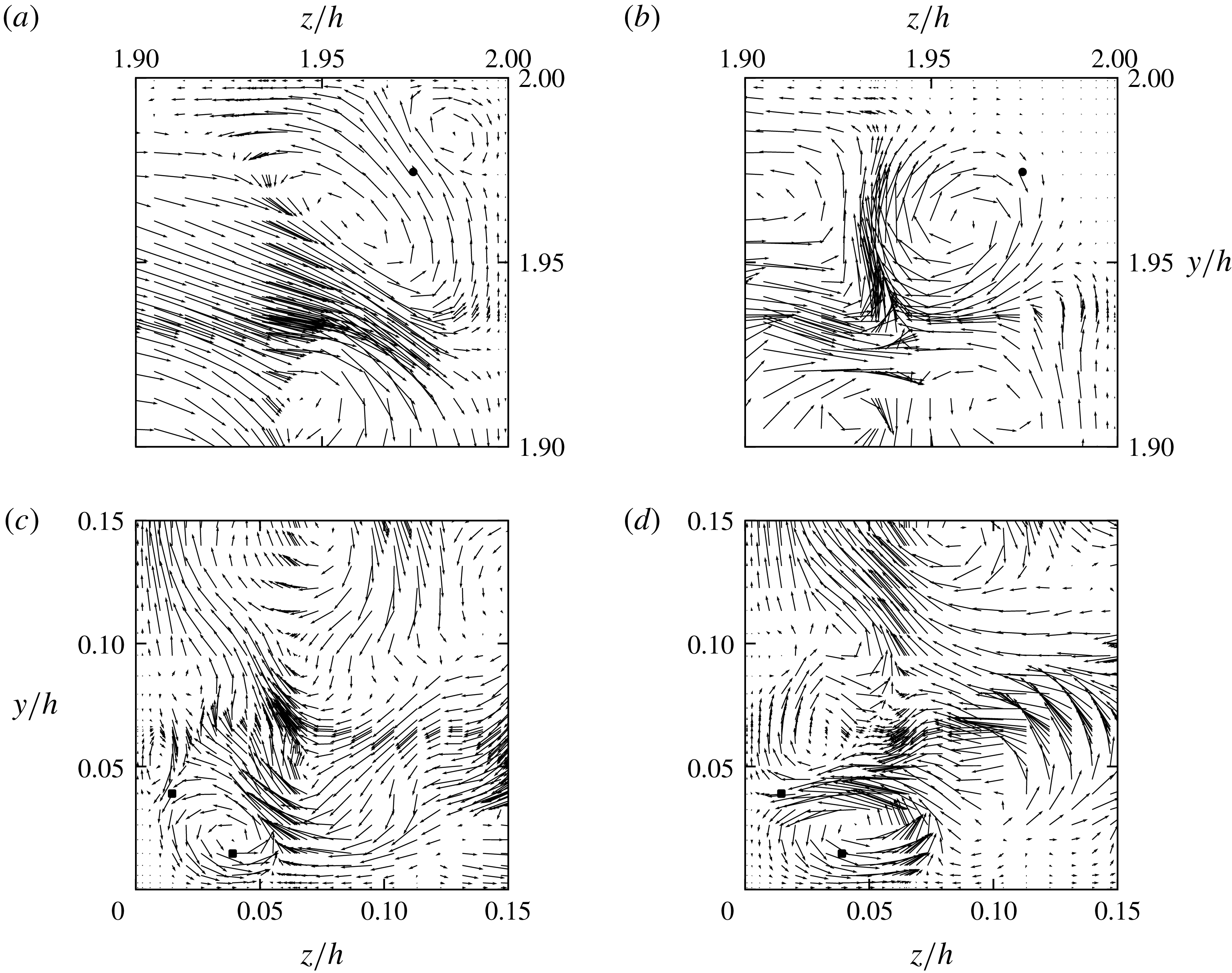
Instantaneous
 $v$
–
 $w$
vectors on a reduced set of GLL nodes (half in each direction) in the vicinity of two corners.
 $Re^{+}=861$
. The impression of intense streams is due to node clustering near element boundaries. (a,b) Flow near the
 $y=z=2h$
corner. The latter plane is 228 wall units downstream of the former. The black dots mark the position of the inflection point of
 $U(y=z)$
(on the diagonal.) (c,d) Flow near the
 $y=z=0$
corner. The streamwise separation between the two planes is 60 wall units. The two black squares on each plane mark the positions of the maximum and minimum of the mean vorticity production term
 $T_{2}$
in definition (6.2).

An instability linked to the mean profile of the corner flow has a good chance of being observed in the instantaneous field data. In this relatively quiescent part of the flow field where large-scale outer motions are predominantly suppressed, a set of distinct and recurring flow events are observed. The views shown in figure 8 are not rare and do not need special extraction methods, but they are easily accessible from most of the database files and it is especially so for the three lower Reynolds numbers, where they constitute the dominant part of the secondary flow field. Most of the instantaneous velocity fields will show a near-corner relatively asymmetric secondary flow pattern with mere streamwise averaging.
The first possible source appears to be around the inflection point on the diagonal profile of
 $U(y,z)$
. Figure 8(a,b) shows the same-instant velocity on two transverse planes close to the top-right corner; plane (a) is 228 wall units upstream of plane (b). The cross-flow in the former contains two unequal counter-rotating vortices stacked into the corner and divided quite symmetrically by the diagonal, but this pattern is not as common as its more asymmetric but rapidly evolving variants. This less unstable instance enables a meaningful quantitative comparison, which allows us to gauge the lower end of the growth process. In the upstream state, plane (a), the velocity ratio of the two adjacent vortices is about two, which would exclude the slow process of viscous diffusion as in Moffat (Reference Moffat1964). The smaller vortex wedged into the corner behind the inflection mark is found growing in every one of the downstream planes (not shown) leading to the stronger vortex in plane (b) whose circumferential velocity is about 2.5 times that of its concurrent upstream part. Thus, it seems likely that the profile around the inflection point is susceptible to (nonlinear) vortex generation and growth. Under the influence of its three image vortices about the corner walls, it will (self-) convect away from the corner in a direction compatible with the mean secondary flow pattern. However, the main contributor to the near-corner secondary flow by far is the type of instantaneous velocity shown in the simultaneous views in figure 8(c,d). For
 $Re^{+}=861$
, the areas near each corner wall and
 $0.05h$
(
 ${\sim}43\unicode[STIX]{x1D708}/u_{\unicode[STIX]{x1D70F}}$
) from the corner itself are particularly susceptible to vortex generation. Even under relatively brief and seemingly quiescent conditions, a vortex can be found being generated well clear of the inflection point on the diagonal, followed by rapid downstream growth and almost invariably the generation of a counter-rotating vortex on the side wall as captured in figure 8(c). Downstream, plane (d), the original vortex has strengthened while moving away from the corner, and the newly created one on the other wall has grown and strengthened as well. Occasionally, the two may grow close to the pro forma symmetric pair expected from the mean cross-flow, or more often, asymmetrically with the dominant one – could be either of the two – quite often appearing to trigger another generation process similar to that of the upstream plane (c). Up to three consecutive cycles of this type have been observed coexisting in the data. Ahead of the contact the downflow of these vortices makes with each corner wall, the maximum or minimum of the turbulent vorticity intensification production term (
 $T_{2}$
, see definitions (6.2)) of the mean vorticity equation is situated. This is the subject of the mean streamwise vorticity section.
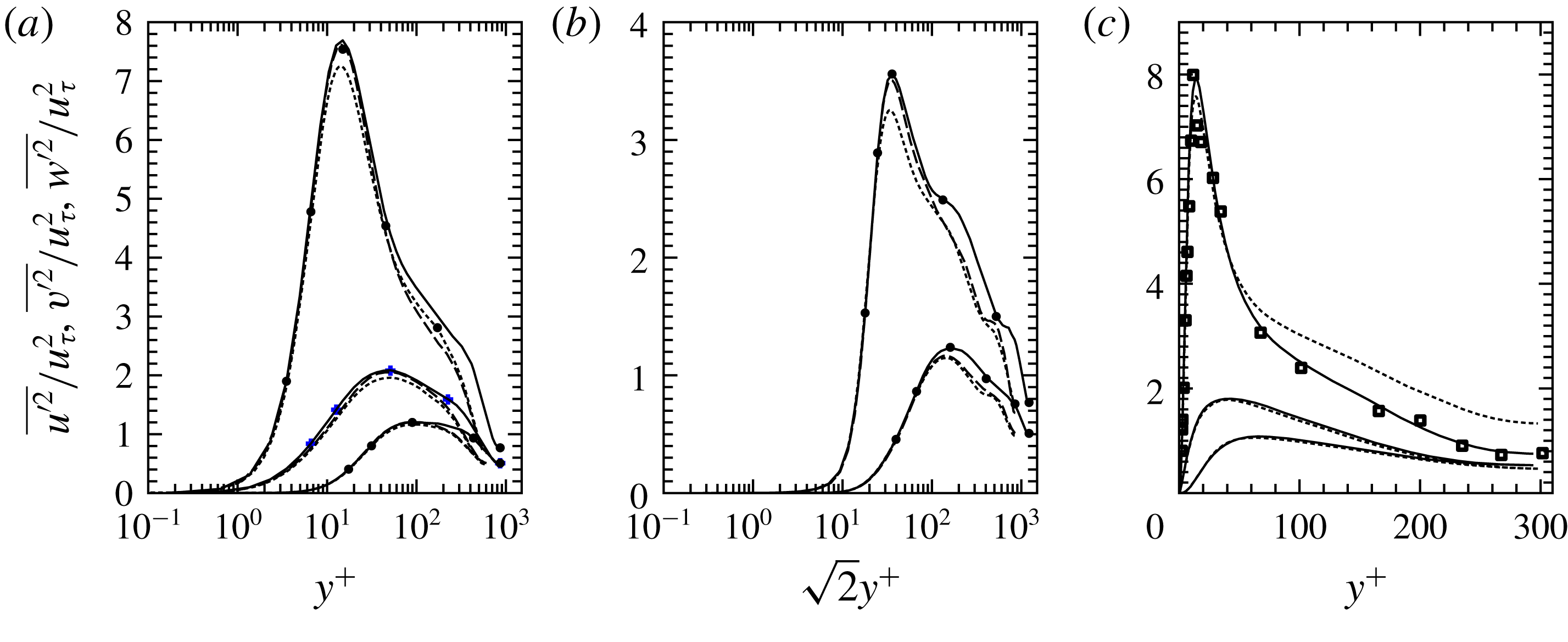
Turbulent velocity intensities: (a,b) ——,
 $Re^{+}=861$
; — — —,
 $Re^{+}=605$
; - - - -,
 $Re^{+}=600$
from Zhang et al. (Reference Zhang, Trias, Gorobets, Tang and Oliva2015). (a) Along the wall bisector. The topmost group is for
 $u^{\prime }$
followed by
 $w^{\prime }$
and
 $v^{\prime }$
(normal component). Markers show the values of the intensities for
 $Re^{+}=861$
averaged over the shorter interval of
 $10.6h/u_{\unicode[STIX]{x1D70F}}$
. (b) Along the diagonal: top group, intensities of
 $u^{\prime }$
; lower group,
 $v^{\prime }$
or
 $w^{\prime }$
. Markers are used as in (a). (c) Wall bisector: ——,
 $Re^{+}=295$
of table 1; - - - -,
 $Re^{+}=300$
from Zhang et al. (Reference Zhang, Trias, Gorobets, Tang and Oliva2015); ▫,
 $\overline{{u^{\prime }}^{2}}/u_{\unicode[STIX]{x1D70F}}^{2}$
for
 $Re_{m}=10000$
(
 $Re^{+}\sim 307$
) from Yong (Reference Yong1988). The three components are grouped and ordered as in (a).

5 Turbulent kinetic energy
Due to the mixed origins of the cross-flow velocities in general, the three intensities would not be expected to scale until the Reynolds number is sufficiently high for the influence of the corners on the bulk flow to have considerably waned. These higher Reynolds number effects are evident for parts of the flow field and a restricted scaling for the turbulent intensities appears to be present. In figure 9(a,b), the variation of intensities on two symmetry axes from the two highest Reynolds numbers of the present report are shown together with the relevant data from the
 $Re^{+}=600$
duct simulation of Zhang et al. (Reference Zhang, Trias, Gorobets, Tang and Oliva2015). For the current results, scaling with the global friction velocity (
 $u_{\unicode[STIX]{x1D70F}}$
) produces good agreement between the three intensity components up to and a little beyond their respective peak values along the wall bisector. The corresponding data of Zhang et al. (Reference Zhang, Trias, Gorobets, Tang and Oliva2015) show lower peak values for the streamwise and
 $w^{\prime }$
components, but agree quite well on the positions of the three maxima. The spectra of the present data at the peak locations show negligible build-up of high-wavenumber energy in all three intensity components; typical small-scale accumulation can be seen in figure 2(a,b). Both
 $Re^{+}\sim 600$
simulations have the same
 $L_{x}$
, and therefore differences due to sampling any unresolved long wavelengths cannot be the cause. The data here include the zero wavenumber (fluctuation) intensities, but these cannot account for the differences. The nominal cross-flow grid resolution in Zhang et al. (Reference Zhang, Trias, Gorobets, Tang and Oliva2015) is excellent with the streamwise grid spacing about 18 % larger than the present and this might explain the differences. An additional comparison between intensities can be made due to their proximity in
 $Re$
when
 $Re^{+}\sim 300$
(figure 9
c), where the streamwise ratio
 $L_{x}/h$
used here is 2.5 times larger. The transverse intensity components from the two simulations agree quite well. But the scaled maximum of
 $\overline{{u^{\prime }}^{2}}$
in Zhang et al. (Reference Zhang, Trias, Gorobets, Tang and Oliva2015) is still less than that of the present data, and strangely it shows quite high values over the core part,
 $y^{+}>60$
, of the duct. Near the duct centre, the Zhang et al. (Reference Zhang, Trias, Gorobets, Tang and Oliva2015) data are about 80 % higher than those of the
 $Re^{+}=295$
simulation; at this
 $Re^{+}$
, the Zhang et al. (Reference Zhang, Trias, Gorobets, Tang and Oliva2015) simulation is still susceptible to the effects of the short
 $L_{x}$
. The measurements of Yong (Reference Yong1988) for
 $Re_{m}=10\,000$
appear to agree quite well with the present simulation from the wall up to the peak of
 $\overline{{u^{\prime }}^{2}}$
; following this, there is a steep drop in the next experimental point beyond which experiment and simulation agree quite well again. Note that the peak value of
 $\overline{{u^{\prime }}^{2}}/u_{\unicode[STIX]{x1D70F}}^{2}$
for
 $Re^{+}=295$
is larger than those of
 $Re^{+}=605$
and
 $861$
. This is due to the spatial displacement trend with
 $Re$
of the global maximum of turbulent kinetic energy away from the wall bisector, which is discussed later in this section.
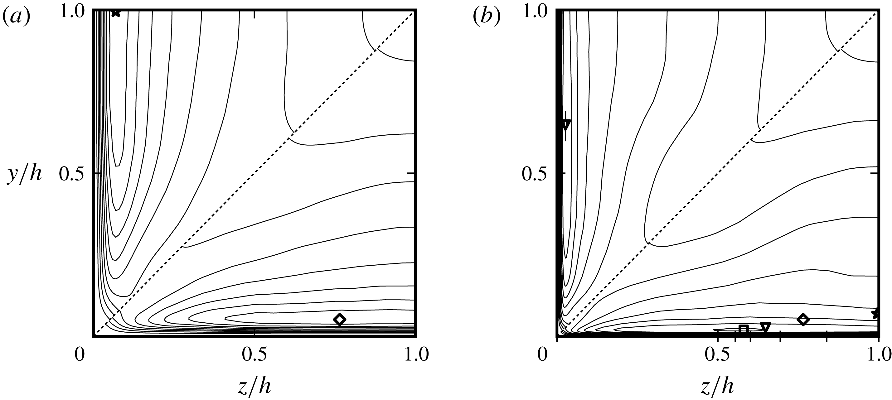
Mean turbulent kinetic energy scaled with
 $u_{\unicode[STIX]{x1D70F}}^{2}$
for four Reynolds numbers. (a) Above the diagonal,
 $Re^{+}=215$
; below,
 $Re^{+}=295$
. (b) Above the diagonal,
 $Re^{+}=605$
; below,
 $Re^{+}=861$
. The interval between adjacent contours is
 $0.5u_{\unicode[STIX]{x1D70F}}^{2}$
. Each marker shows the location of the maximum for the different Reynolds numbers. In the
 $Re^{+}=861$
octant, all four markers are included. Each of the four unlabelled tickmarks after
 $z/h=0.5$
in (b) shows the location of the maximum dissipation rate for the different
 $Re$
: the leftmost unlabelled tickmark is for
 $Re^{+}=861$
; subsequent ones are in order of decreasing
 $Re$
.

The good agreement between the intensities for the two highest
 $Re^{+}$
on the wall bisector when scaled with the global friction velocity rather than the local measure of it, is consistent with the finding that there are very long oblique wall structures spanning most of the width of the duct. In this case, the corner influence reaching some mid-wall portion of the flow would have originated well upstream of it, and while it would be developing a degree of decorrelation and intermittency, the global scale would still appropriately reflect its upstream-corner provenance; this will evidently fade with increasing
 $Re$
. The upstream influence near the wall bisector reappears in the source term(s) of the mean vorticity in § 6.
The peak intensity of
 $u^{\prime }$
on the corner bisector is at
 $y^{+}=z^{+}\sim 25$
– about half-way between the corner and the peak of the secondary velocity – where the skewness of
 $u^{\prime }$
is positive and relatively high (about 3, not shown) suggesting that intermittent inrush of high-speed fluid from the outer flow may well be the main contributor to the near-corner maximum of intensity. This also conforms with the effects of the flow description attached to figure 8(c,d) and consequent lack of scaling in
 $k$
.
The distribution of the turbulent kinetic energy
 $k$
over the cross-section (figure 10) allows an overview of the evolution of turbulence with the Reynolds number. Starting at the mid-plane when
 $Re^{+}=215$
, the overall maximum of
 $k$
,
 $k_{max}$
, has moved closer to
 $z=0.5h$
when
 $Re^{+}=861$
; see marks in the lower octant of figure 10. Initially, the low
 $Re^{+}$
peak is relatively isolated and on the wall bisector, but becoming broader in the wall-parallel direction while remaining at an approximately constant distance from the nearest wall in nominal wall units. The position of
 $k_{max}$
close to the wall appears to be determined by the proximity of the corner following some (unknown) relation, but the available range of
 $Re$
is not yet high and wide enough to detect any scaling behaviour. The turbulent dissipation rate always has its maximum on the boundaries and usually tracks
 $k_{max}$
, which normally coincides with the maximum of turbulent energy production. However, there is a rather large gap between
 $k_{max}$
and its companion wall maximum of
 $\unicode[STIX]{x1D716}$
when
 $Re^{+}=215$
or 295, and therefore the notion of approximate local equilibrium would not be applicable, making scaling in local variables for low
 $Re$
unlikely.
6 Mean streamwise vorticity
The two well-separated secondary velocity troughs along the corner bisector for the higher
 $Re^{+}$
suggest distinct driving mechanisms. The turbulent flow origins of the outer one may be indirectly accessed through the equation for the mean streamwise vorticity,
 $\unicode[STIX]{x1D6FA}_{x}=\unicode[STIX]{x2202}W/\unicode[STIX]{x2202}y-\unicode[STIX]{x2202}V/\unicode[STIX]{x2202}z$
, whose most common form is
 $$\begin{eqnarray}\displaystyle V\frac{\unicode[STIX]{x2202}\unicode[STIX]{x1D6FA}_{x}}{\unicode[STIX]{x2202}y}+W\frac{\unicode[STIX]{x2202}\unicode[STIX]{x1D6FA}_{x}}{\unicode[STIX]{x2202}z}=\text{}\underline{\frac{\unicode[STIX]{x2202}^{2}}{\unicode[STIX]{x2202}y\unicode[STIX]{x2202}z}(\overline{{v^{\prime }}^{2}}-\overline{{w^{\prime }}^{2}})+\left(\frac{\unicode[STIX]{x2202}^{2}}{\unicode[STIX]{x2202}z^{2}}-\frac{\unicode[STIX]{x2202}^{2}}{\unicode[STIX]{x2202}y^{2}}\right)\overline{v^{\prime }w^{\prime }}}+\unicode[STIX]{x1D708}\left(\frac{\unicode[STIX]{x2202}^{2}}{\unicode[STIX]{x2202}y^{2}}+\frac{\unicode[STIX]{x2202}^{2}}{\unicode[STIX]{x2202}z^{2}}\right)\unicode[STIX]{x1D6FA}_{x}.\quad & & \displaystyle\end{eqnarray}$$
A substantial advantage of using this equation is that it has no terms mixing mean-field and turbulent variables. If either the
 $y$
or
 $z$
direction were to become homogeneous, then both turbulent terms in (6.1) would be zero. This suggests the likely limiting behaviour with increasing Reynolds number of the duct flow over a broadening stretch centred on each mid-plane as the effects of the mean vorticity sources gradually scale down toward each corner. Any approximate homogeneity about the wall bisector at lower Reynolds numbers is due to the fortuitous cancellation required by symmetry constraints, and channel-like statistics are not to be expected. The two highest Reynolds numbers here have not reached a quasi-homogeneous state around the mid-walls with the outer cross-flow velocity maximum still changing and the distance separating the corner peak from the main-flow one of each of two curves in figure 7(b) still evolving.
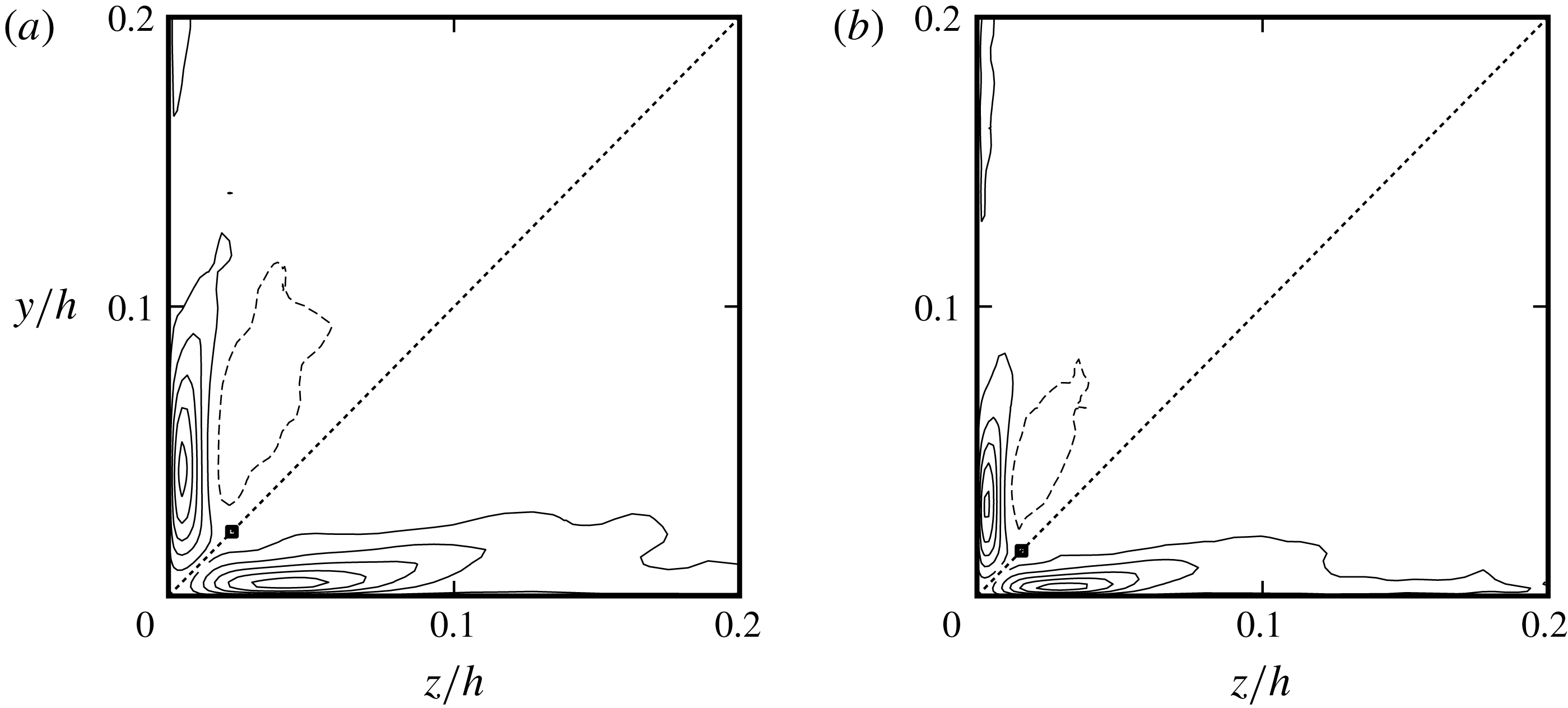
Source terms of the equation for the mean streamwise vorticity in their Reynolds stress form. Below each bisector,
 $\unicode[STIX]{x2202}^{2}(\overline{{v^{\prime }}^{2}}-\overline{{w^{\prime }}^{2}})/\unicode[STIX]{x2202}y\unicode[STIX]{x2202}z$
; above,
 $(\unicode[STIX]{x2202}^{2}/\unicode[STIX]{x2202}z^{2}-\unicode[STIX]{x2202}^{2}/\unicode[STIX]{x2202}y^{2})\overline{v^{\prime }w^{\prime }}$
. Both terms are normalized with their overall maximum magnitude. Solid lines denote positive contour values, dashed lines negative values. All terms have the signs appropriate for the octant they are shown in. Successive contours differ by 0.2. Contour range
 $[-0.9,0.9]$
. The square marks are the inflection points of
 $U(y,z)$
on the diagonals. (a)
 $Re^{+}=605$
. (b)
 $Re^{+}=861$
.

6.1 Reynolds stress form
Like all other duct statistics, the mean vorticity and associated correlations will adapt to the symmetries of the bounding geometry whose basic constituent is an octant. For every pair of adjacent octants,
 $\unicode[STIX]{x1D6FA}_{x}$
and every term in (6.1) will be antisymmetric with respect to their common boundary on which their values must be zero. In the
 $\{z\leqslant h;y\leqslant z\}$
– or lower left – octant the vorticity at the centre of the large vortex, as in figure 7(a), will be negative whereas near and at the wall it is positive and on the two internal symmetry lines zero (figure 12
a upper octant but with a reversed sign). The magnitude of the overall maximum of
 $\unicode[STIX]{x1D6FA}_{x}$
which occurs on the walls, is more than 25 times that at the centre of the secondary vortex in figure 7(a). It is significant that high values of
 $\unicode[STIX]{x1D6FA}_{x}$
extend over most of the duct wall, which indicates a distributed generation mechanism whose origin must be traced to the effects of the corners. In terms of the mean velocity field, it consists of generating a net velocity component close and parallel to the no-slip wall, which drives the flow within a triangle on whose two internal boundaries free-slip conditions apply.
The distributions of the two turbulent terms over part of the cross-section for
 $Re^{+}=861$
and
 $605$
are shown in figure 11. It needs to be remembered here that spectral element computations do not enforce continuity of higher-order velocity derivatives at the inter-element boundaries, but they converge toward such continuity with increasing resolution. With restricted spatial resolution and depending on the local state of the flow, boundary values of such derivatives from one element may differ from those calculated from the adjoining element since each covers a different part of the flow domain. Here, the common-boundary values for the expressions of the turbulent source in (6.1) and
 $T_{1}$
in definitions (6.2) below are assigned the estimate from whichever of the adjoining elements is closest to the average of their boundary-adjacent nodes.
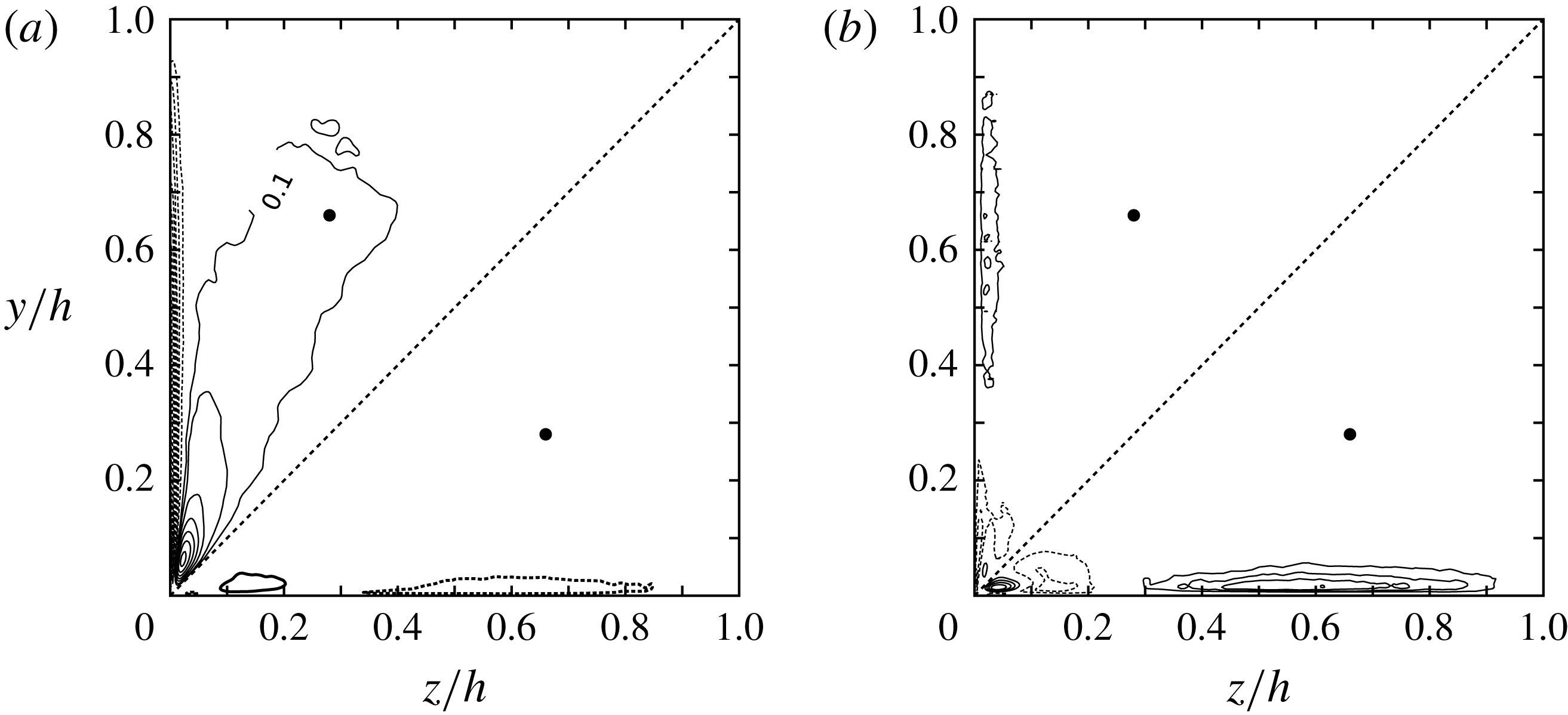
Mean streamwise vorticity
 $\unicode[STIX]{x1D6FA}_{x}$
and the source terms of its equation in the vorticity form (6.2) for
 $Re^{+}=861$
. (a) Above the diagonal,
 $h\unicode[STIX]{x1D6FA}_{x}/U_{m}$
; below, turbulent vorticity shearing
 $T_{3}$
. (b) Above the diagonal, turbulent transport
 $T_{1}$
; below, intensification of
 $\unicode[STIX]{x1D714}_{x}^{\prime }$
,
 $T_{2}$
. The
 $T$
-terms are scaled with the maximum of
 $|T_{2}|$
. The interval between adjacent
 $T$
contours is
 $0.2$
; the maximum positive contour is
 $0.8$
. Mean vorticity intervals
 $0.2U_{m}/h$
with range [
 $-3.4,1.4$
]. The additional contour marked 0.1 is 37 times smaller than the absolute maximum on the wall. Zero contour lines are not shown. Positive values are drawn with solid lines, negative with dotted. All four quantities have the correct sign for the octant they are drawn in; they would change sign on being reflected about the diagonal. The filled symbols show the centre of the secondary flow.

For both
 $Re^{+}$
, the terms containing the Reynolds stresses attain their peak (absolute) values very close to the corner with marked overlap. The maximum value of the anisotropy term exceeds that of the shear stress term by about 6 % and they can be assumed to both be mostly related to the near-corner part of the secondary flow. In the same octant, the two terms are largely of opposite sign, resulting in substantial cancellation which tends to lessen with increasing Reynolds number. Due to imperfect overlap, the maximum of their sum when
 $Re^{+}=861$
is about half the peak value of either. This would suggest that the two turbulent terms in (6.1) are unlikely to originate in independent flow processes at least near their peak values. Firm analytical support for this is embedded in the derivation of the ‘stretching’,
 $T_{2}$
, and ‘tilting’,
 $T_{3}$
, terms that are used in the next subsection; each one is formed from products of velocity derivatives drawn from both turbulent terms of (6.1). These are statistics of the nominal generation process associated with flow events such as those shown in figure 8(c,d). Farther from the corner,
 $z>0.3h$
(not shown), the turbulent terms have and add up to low values, leaving their dynamical significance unclear.
Averaging is a linear operation, and therefore the unbarred form of the turbulent terms may be used to locate their most intense events within the instantaneous fields. Prominent instances of the turbulent terms in (6.1) within the evolving velocity field are outlined here with an alternative view in terms of the turbulent vorticity to follow. The description is based on the
 $Re^{+}=861$
data in order to minimize the inclusion of any lingering very low Reynolds number effects in addition to having the largest available inner–outer cross-flow separation. High instantaneous (absolute) values of both turbulent terms are more than an order of magnitude larger than their respective maximum or minimum mean values drawn in figure 11. Unusually high values are rarely seen near the corners despite their averages having their extrema there. They are found mainly closer to the rim of vortices rather than their centres, in shear layers turning under the blocking influence of the walls and on wall-parallel shear layers when detaching. The common traits of the instantaneous velocity field that underlie the turbulent terms in (6.1) are significant instantaneous streamline curvature and large values of
 $v^{\prime }$
and
 $w^{\prime }$
, and therefore, where the cross-plane velocity vector is inclined about
 $45^{\circ }$
to the nearby boundary. These can occur over a broad strip around the duct perimeter. High instantaneous values for these terms have not been observed near the duct centre. They are particularly marked where vortices are generated at the walls including near the corners. The Reynolds stress form of the
 $\unicode[STIX]{x1D6FA}_{x}$
equation emphasizes statistical aspects of the turbulent velocity field rather than precise dynamical processes, which are difficult to interpret as its two generating terms overlap over the same flow events and which is reflected on their averaged distribution. For the two highest Reynolds numbers, their maxima/minima occur around 26 wall units from the nearest side wall and 3.2 wall units above the nearest ‘horizontal’ one. They are related to vortices whose downflow almost touches one corner wall and impinges on the other as in figure 8(c,d). Both the well-defined position and scaling of these suggest flow instabilities specific to the mean profile close to the corner.
6.2 Turbulent vorticity form
A more incisive way of obtaining the information contained in the terms due to turbulence of (6.1) is to replace their sum by an expression of three terms coupling the turbulent vorticity components
 $\unicode[STIX]{x1D714}_{x}^{\prime }=\unicode[STIX]{x2202}w^{\prime }/\unicode[STIX]{x2202}y-\unicode[STIX]{x2202}v^{\prime }/\unicode[STIX]{x2202}z$
,
 $\unicode[STIX]{x1D714}_{y}^{\prime }=\unicode[STIX]{x2202}u^{\prime }/\unicode[STIX]{x2202}z-\unicode[STIX]{x2202}w^{\prime }/\unicode[STIX]{x2202}x$
,
 $\unicode[STIX]{x1D714}_{z}^{\prime }=\unicode[STIX]{x2202}v^{\prime }/\unicode[STIX]{x2202}x-\unicode[STIX]{x2202}u^{\prime }/\unicode[STIX]{x2202}y$
and fluctuating velocity. Using the continuity equation and flow homogeneity in
 $x$
, the Reynolds stress terms can be replaced by the sum of
 $$\begin{eqnarray}\displaystyle T_{1}=-\left(\overline{v^{\prime }\frac{\unicode[STIX]{x2202}\unicode[STIX]{x1D714}_{x}^{\prime }}{\unicode[STIX]{x2202}y}}+\overline{w^{\prime }\frac{\unicode[STIX]{x2202}\unicode[STIX]{x1D714}_{x}^{\prime }}{\unicode[STIX]{x2202}z}}\right),\quad T_{2}=2\overline{\unicode[STIX]{x1D714}_{x}^{\prime }\frac{\unicode[STIX]{x2202}u^{\prime }}{\unicode[STIX]{x2202}x}},\quad T_{3}=\left(\overline{\unicode[STIX]{x1D714}_{y}^{\prime }\frac{\unicode[STIX]{x2202}u^{\prime }}{\unicode[STIX]{x2202}y}}+\overline{\unicode[STIX]{x1D714}_{z}^{\prime }\frac{\unicode[STIX]{x2202}u^{\prime }}{\unicode[STIX]{x2202}z}}\right)\!.\quad & & \displaystyle\end{eqnarray}$$
Unlike the Reynolds stress form, expressions (6.2) represent three distinct vorticity processes where the first two terms show how
 $\unicode[STIX]{x1D714}_{x}^{\prime }$
can be added to (or subtracted from)
 $\unicode[STIX]{x1D6FA}_{x}$
: turbulent transport in the presence of gradients and vorticity intensification. The last term,
 $T_{3}$
, is of the type that characterizes the origin of Prandtl’s secondary flows of the first kind representing the shearing of the two transverse vorticity components. The first term,
 $T_{1}$
, is in a sense passive; it transports pre-existing vorticity when gradients are present and it would be significant at the point where the generation of
 $\unicode[STIX]{x1D714}_{x}^{\prime }$
is intense and highly localized in the absence of other competing processes. It appears mostly as a source close to the corner and as a sink term farther toward the mid-wall (figure 12
b upper octant). The term
 $T_{2}$
, whose dynamically concise and precise form depends on the incompressibility (2.2), is the main source along the smooth duct wall and attains high values close to the boundaries where both direct generation of
 $\unicode[STIX]{x1D714}_{x}^{\prime }$
and intense normal strains from the deflection of high-speed downflows occur.
To assess the relative contribution of each term, the distribution of
 $\unicode[STIX]{x1D6FA}_{x}$
over the same area has to be considered. This is drawn in figure 12(a), upper octant, keeping in mind that it and the
 $T$
-terms are antisymmetric about the diagonal. All comparisons that follow are based on the signs appropriate over the lower octant, where the mean vorticity has a positive maximum at the wall and the secondary flow vortex sense of rotation corresponds to negative vorticity. Numerically, the near-wall vorticity is an order of magnitude larger than the value at the centre of the secondary vortex. Unsurprisingly, the
 $T$
-terms attain their highest values where
 $\unicode[STIX]{x1D6FA}_{x}$
is large and away from the corner it is the region of high positive values close to the wall. From figure 12,
 $T_{1}$
and
 $T_{3}$
are mainly sink terms and
 $T_{2}$
is numerically the largest and effectively the only source. It is the sum of the three terms over the region
 $\unicode[STIX]{x1D6FA}_{x}>0$
that underlies the outer secondary flow, but now the dynamical process of mean vorticity generation has been identified. The highest overall
 $T_{2}$
value is found close to the corner and it marks the position where it is most likely that the vortices generated near the corner will produce significant positive contributions to it and reflects the more organized state of this part of the flow. It is now possible to directly associate the instantaneous flow field in figure 8(c,d) with the maximum and minimum of
 $T_{2}$
. The corner extrema are found on the ‘downflow’ side of the larger corner vortex in figure 8(c), once where it impinges on the side wall generating the new small vortex and a second time while the vortex flow is turning due to blockage of the near wall; they re-emphasize the importance of streamline curvature noted earlier. These types of events are expected to be contributing to the generation processes father away from the corner, with the difference that the likelihood of seeing vortices of one sign or the other evens out. These findings are applicable to square ducts with smooth walls and most likely to rectangular ducts of other aspect ratios. However, it is possible that
 $T_{3}$
will appear as a contributing source of secondary flow vorticity within turbulence near corners of angles other than
 $90^{\circ }$
with or without graded wall roughness.
The question that remains is how to account for the influence of the corner geometry propagating toward the mid-wall giving rise to the elongated
 $T_{2}$
contours for
 $z>0.3h$
with very mild tapering, but abrupt end toward the mid-wall. In addition, there is a noticeable gap around
 $z=0.25h$
in the
 $T_{2}$
contours, and directly above it on the diagonal is the area of the maximum between the two negative velocity troughs in figure 7(b,c). This gap could conceivably be attributed to statistical cancellation between near- and far-corner events, but there is no symmetry point or line nearby and similar gaps are found in the remaining
 $T$
-terms, each representing different vorticity processes. A plausible explanation for both features is suggested by figure 4(a,b), where long oblique structures span a large fraction of the wall. Based on this observation, the twofold structure of the secondary flows for the two highest
 $Re$
may be constructed as the composite of a near-corner component driven by a mean-field instability producing short-lived relatively localized vortices, and of another with very long and long-living structures most evident in the form of oblique near-wall streaks of
 $u^{\prime }$
originating well upstream and possibly reaching the opposite side wall for the current
 $Re$
. The former is well supported by the statistics and instantaneous views of the velocity field while the latter is more of a conjecture that fits the available data well. Within the framework of this explanation, the slight tapering of the
 $T_{2}$
contours toward the wall centre can be accounted for by symmetry considerations. The mean vorticity generation due to one corner would normally extend beyond the mid-wall, but it encounters a similar but opposite-signed process from the other corner and an antisymmetry constraint about the wall bisector on which
 $T_{2}=0$
.
The near-corner secondary velocity component has been linked directly to the corner mean velocity profile instability and therefore does not fit well into Prandtl’s twofold classification of secondary flows. It is the dominant form for
 $Re^{+}$
below approximately 300, but with increasing Reynolds number it becomes confined to ever smaller regions around each corner, with its maximum seemingly at a constant distance from its walls in
 $\unicode[STIX]{x1D708}/u_{\unicode[STIX]{x1D70F}}$
units. The confined state of this secondary flow component for the highest
 $Re$
is also evident in the isolation and compactness of the
 $T_{2}$
contours close to the corner in figure 12(b).
Sufficiently near the
 $y$
-wall
 $\unicode[STIX]{x1D714}_{x}^{\prime }\sim \unicode[STIX]{x2202}w^{\prime }/\unicode[STIX]{x2202}y$
. The two remaining factors in
 $T_{2}$
are then also contributors to the turbulent dissipation rate, and therefore, away from the corner, the mean vorticity generation may be viewed as being due to a subset of the dissipative motions of near-wall turbulence. Furthermore, the instability-driven part of the secondary flow extracts its energy from the mean flow field, whereas for the outer part, the proximate source of its energy is turbulent motions, and therefore this process may be termed negative turbulence production.
7 Conclusion
The present simulations highlight the unsettled character of the square duct flow with respect to changes in the low Reynolds number range with no indication of whether and how far it will persist with farther increases in the Reynolds number. The friction Reynolds numbers up to about 300 are quite special. Based on the mean streamwise vorticity equation, the dominant source mechanism of the secondary flows appears at specific sites near each corner wall where a recurring vortex generation sequence at these locations is observed; this points to generation by mean flow instability. With increasing Reynolds number, this mechanism remains dominant, but retreats ever closer to the corner while farther from it, and in the vicinity of the duct walls there emerges a second source site that gradually elongates parallel to the nearest wall, and at higher Reynolds numbers is associated with the larger mean secondary flow. A reflection of the double-structure source is two peaks in the transverse velocity magnitude along the diagonal where the statistical influence of each corner wall is the same. The maximum value closest to the corner stays near
 $0.33u_{\unicode[STIX]{x1D70F}}$
while keeping a distance of about 49 wall units from either wall. It appears that neither the friction velocity nor the mean flow velocity will scale the second peak, but the geometric mean of the two is not excluded by the available data. The velocity intensities along the wall bisector, but close to the mid-wall, scale with the friction velocity for
 $Re^{+}=605$
and
 $861$
. It may be more than mere coincidence that this limited scaling is found first in flows whose energy dissipation in the turbulent field matches or exceeds that of their mean field.
Only the outer part of each secondary flow is due to incompressible turbulence at higher Reynolds numbers; it is the end result of three distinct vorticity processes where two of them, turbulent vorticity transport and shearing, nearly deplete the principal generation mechanism: net streamwise vorticity intensification. The latter is usually thought of as the turbulent energy transfer mechanism to smaller scales and viscous dissipation, but in an inhomogeneous environment, it can channel turbulent energy upscale – to the mean flow.
Acknowledgements
Thanks are due to Emmanuel Leriche of Université de Lille 1, France, and Helen Theodoropoulou of Harokopio University, Athens, Greece.