1 Introduction
Flow regime prediction of multiphase flows in confined geometries is important for many engineering techniques and industrial processes, and it remains a challenging problem in fundamental fluid mechanics (Brennen Reference Brennen2005; Crowe Reference Crowe2006; Cheng, Ribatski & Thome Reference Cheng, Ribatski and Thome2008). Flow patterns can indeed adopt various interfacial morphologies and dynamics, leading to diverse mechanisms for the transport of mass, momentum and energy (Bird, Stewart & Lightfoot Reference Bird, Stewart and Lightfoot2002). While the motion of a single-phase flow depends on the interplay between inertial and viscous forces, the behaviour of two-phase flows involves numerous parameters, including bulk fluid properties, such as densities and viscosities, and interfacial properties, such as surface tension. In addition, flow destabilization processes also depend on flow parameters and local geometries, including Plateau–Rayleigh instabilities, where liquid threads break into droplets due to interfacial tension, Kelvin–Helmholtz instabilities between streams having large differences in velocities, Rayleigh–Taylor instabilities for heavier fluids sitting on top of lighter ones, and Saffman–Taylor instabilities when a less viscous fluid is injected through a thick fluid in confined geometries (Drazin & Reid Reference Drazin and Reid2004). In general, hydrodynamic stability analysis of open flows includes (a) convective instabilities, where flow perturbations are advected downstream, and (b) absolute instabilities, where perturbations can also propagate upstream (Huerre & Rossi Reference Huerre and Rossi2005; Salin & Talon Reference Salin and Talon2019). Linear stability analysis of base flow provides a useful framework for determining regions of stability and flow characteristics; however, less is known about the evolution of fluid morphologies and pattern dynamics at the transition between flow regimes.
Owing to considerable industrial interest, liquid–gas flows have been significantly studied in channels of various sizes and a wide range of flow patterns have been classified, such as bubbly, slug, churn, stratified, wavy, mist and core–annular flows (Triplett et al. Reference Triplett, Ghiaasiaan, Abdel-Khalik and Sadowski1999; Cubaud, Ulmanella & Ho Reference Cubaud, Ulmanella and Ho2006; Berna et al. Reference Berna, Escrivá, Munoz-Cobo and Herranz2015). Multiphase flow patterns can also be grouped into two categories: (a) dispersed flows, where one phase forms discrete elements in the other continuous phase, and (b) separated flows, where both phases form continuous streams (Crowe Reference Crowe2006). A difficulty in predicting regime selection of dispersed and separated flows lays in the different methods used to analyse each flow pattern, and a unifying approach would improve predictive knowledge of multiphase flows.
Microfluidic technologies provide advanced experimental platforms with fine control over flow rates and microgeometries to investigate the role of fluid properties in multiphase flow instabilities (Hu & Cubaud Reference Hu and Cubaud2018). For liquid–liquid systems, monodisperse droplet dispersions can be steadily generated using microchannels and find use to encapsulate reagents in domains as diverse as material synthesis, drug discovery and the food industry (Barrero & Loscertales Reference Barrero and Loscertales2007; Baroud, Gallaire & Dangla Reference Baroud, Gallaire and Dangla2010; Anna Reference Anna2016; Evangelio, Campos-Cortés & Gordillo Reference Evangelio, Campos-Cortés and Gordillo2016; Mowlavi et al. Reference Mowlavi, Shukla, Brun and Gallaire2019). Two common regimes of droplet formation have been identified as dripping and jetting based on the location of droplet pinch-off from the fluid junction (Eggers Reference Eggers1997; Guillot et al. Reference Guillot, Colin, Utada and Ajdari2007; Cubaud & Mason Reference Cubaud and Mason2008; Nunes et al. Reference Nunes, Tsai, Wan and Stone2013; Gordillo, Sevilla & Campo-Cortés Reference Gordillo, Sevilla and Campo-Cortés2014). The regime transition between dripping droplets, which form in the upstream region near the fluid contactor, and jetting droplets, generated from a slender thread further downstream, corresponds to a shift from an absolute to a convective instability of dispersed flows (Utada et al. Reference Utada, Fernandez-Nieves, Gordillo and Weitz2008; Augello, Fani & Gallaire Reference Augello, Fani and Gallaire2018). Linear stability analysis shows good agreement with data for delineating the absolute–convective instability transition between dripping droplets and jets in coaxial flows (Guillot et al. Reference Guillot, Colin, Utada and Ajdari2007).
In the context of separated flows, the hydrodynamic stability of viscous stratifications has been theoretically and numerically investigated (Yih Reference Yih1967; Hinch Reference Hinch1984; Selvam et al. Reference Selvam, Merk, Govindarajan and Meiburg2007; Govindarajan & Sahu Reference Govindarajan and Sahu2014), and the development of interfacial waves in viscous-stratified flows has been reported in various experimental configurations (Sangalli et al. Reference Sangalli, Gallagher, Leighton, Chang and Mccready1995; Al-Wahaibi & Angeli Reference Al-Wahaibi and Angeli2011; Hu & Cubaud Reference Hu and Cubaud2016). When an inner stream is unsheathed with another fluid, the destabilization of miscible and immiscible core–annular flows has been studied in small tubes with the appearance of interfacial waves (Cao et al. Reference Cao, Ventresca, Sreenivas and Prasad2003), including bamboo waves (Joseph & Renardy Reference Joseph and Renardy1993) and pearl-mushroom waves (D’olce et al. Reference D’olce, Martin, Rakotomalala, Salin and Talon2008), which result from the development of absolute instabilities (Salin & Talon Reference Salin and Talon2019). In microchannels, a variety of instability patterns were examined based on fluid and flow properties during the formation of miscible viscous threads (Cubaud & Notaro Reference Cubaud and Notaro2014). Overall, the development of periodic flow patterns allows one to relate flow characteristics to control parameters and provides insight into hydrodynamic instabilities. A general approach, however, is needed to clarify regime transitions and relationships between dispersed and separated flows in connection with convective and absolute instabilities.
In this article, we examine the microflow behaviour of immiscible fluids having a large difference in viscosity using square focusing sections. A variety of dispersed and separated flows are systematically characterized using a single microflow geometry to compare regimes and determine transitions. In particular, a periodic pattern description is employed to relate wavelength, frequency and celerity of repeating unit cells within each flow pattern based on control parameters. We proceed with the study of dispersed flows and investigate the relationships between dripping and jetting regimes. We then examine separated flows and discuss the development of capillary and inertial waves along core–annular flows. For a given fluid pair, a rich collection of hydrodynamic phenomena is observed from droplet to wave flow regimes. Our analysis shows that the interfacial velocity of base core–annular flow provides a useful reference to compare patterns across flow regimes. We quantify the transition between regimes using dimensionless numbers and demonstrate that both droplet velocity and wave celerity reach a maximum value at the dispersed–separated flow transition. This insight allows us to develop predictive capabilities for the flow transition in good agreement with experimental data over a wide range of viscosity contrasts.
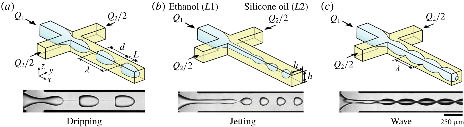
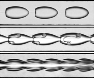
Schematics of typical flow patterns (( $Q_{1},~Q_{2}$), fluid pair) with corresponding experimental micrographs: (a) dripping, ((2, 4),
 $E5\text{h}$); (b) jetting, ((2, 20),
 $E50$); and (c) wavy ((200, 200),
 $E5\text{h}$). Flow rates
 $Q$ in
 $\unicode[STIX]{x03BC}\text{l}~\text{min}^{-1}$. Fluid pairs as in table 1.

Properties of fluids used in experiments, including dynamic viscosity  $\unicode[STIX]{x1D702}$, viscosity contrast
 $\unicode[STIX]{x1D712}^{-1}=\unicode[STIX]{x1D702}_{2}/\unicode[STIX]{x1D702}_{1}$, density
 $\unicode[STIX]{x1D70C}$ and interfacial tension
 $\unicode[STIX]{x1D6FE}_{12}$.

2 Experimental methods
We employ a microfluidic hydrodynamic focusing section that consists of two square microchannels of height  $h=250~\unicode[STIX]{x03BC}\text{m}$ that intersect perpendicularly (figure 1). The microchannel is made of an etched-trough silicon wafer sandwiched between two borosilicate glass plates to allow visualization. Anodic bonding between glass and silicon allows the chip to withstand the large injection pressures associated with the flow of highly viscous liquids in micro-confined environments. The microfluidic platform is mounted on an inverted microscope equipped with a high-speed camera to capture fast interfacial dynamics, and fluids are injected into the device using high-pressure syringe pumps. Droplets and core–annular flows are generated when a fluid
 $L1$ of viscosity
 $\unicode[STIX]{x1D702}_{1}$ is introduced in the central channel at flow rate
 $Q_{1}$ and a more viscous fluid
 $L2$ having a viscosity
 $\unicode[STIX]{x1D702}_{2}$ is symmetrically injected through side channels at total flow rate
 $Q_{2}$. In a typical series of experiments, the flow rate of the high-viscosity fluid
 $Q_{2}$ is fixed and the low-viscosity fluid flow rate
 $Q_{1}$ is varied.
We systematically examine the microflow of three immiscible fluid pairs having low interfacial tension  $\unicode[STIX]{x1D6FE}_{12}$. The liquid
 $L1$ is ethanol and
 $L2$ is silicone oils of various viscosities (table 1). Interfacial tension
 $\unicode[STIX]{x1D6FE}_{12}$ is measured for each fluid pair using the Du Noüy ring method with a high-precision tensiometer. Data show that
 $\unicode[STIX]{x1D6FE}_{12}$ remains nearly constant for large variations of the viscosity ratio
 $\unicode[STIX]{x1D712}=\unicode[STIX]{x1D702}_{1}/\unicode[STIX]{x1D702}_{2}$, which is typically referred to as viscosity contrast
 $\unicode[STIX]{x1D712}^{-1}$ for convenience. Over the range of parameters investigated, the silicone oil
 $L2$ is found to wet the channel walls more than ethanol
 $L1$; therefore the inner fluid is always lubricated by the viscous outer stream.
Depending on fluid properties and flow rates of injections, a range of microflow arrangements are observed in the outlet channel, including (a) dripping, (b) jetting and (c) wave regimes (figure 1). In the dripping regime, droplets are formed near the fluid junction, whereas, in the jetting regime, droplets are generated at the tip of a jet further downstream in the channel. Parameters of interest include the average droplet length  $d$, spacing
 $L$ and velocity
 $V_{D}$. The regularity of droplet flows also enables measurement of wavelength
 $\unicode[STIX]{x1D706}=d+L$ of a unit cell. In the wave regimes, periodic undulations of length
 $\unicode[STIX]{x1D706}$ and celerity
 $c$ develop along the interface formed between the two parallel streams of
 $L1$ and
 $L2$. In the following, we examine the dynamics of each regime and study pattern transition to better understand the relationship between fluid properties and microfluidic multiphase flows in the presence of large viscosity contrasts.
3 Flow regimes and flow maps
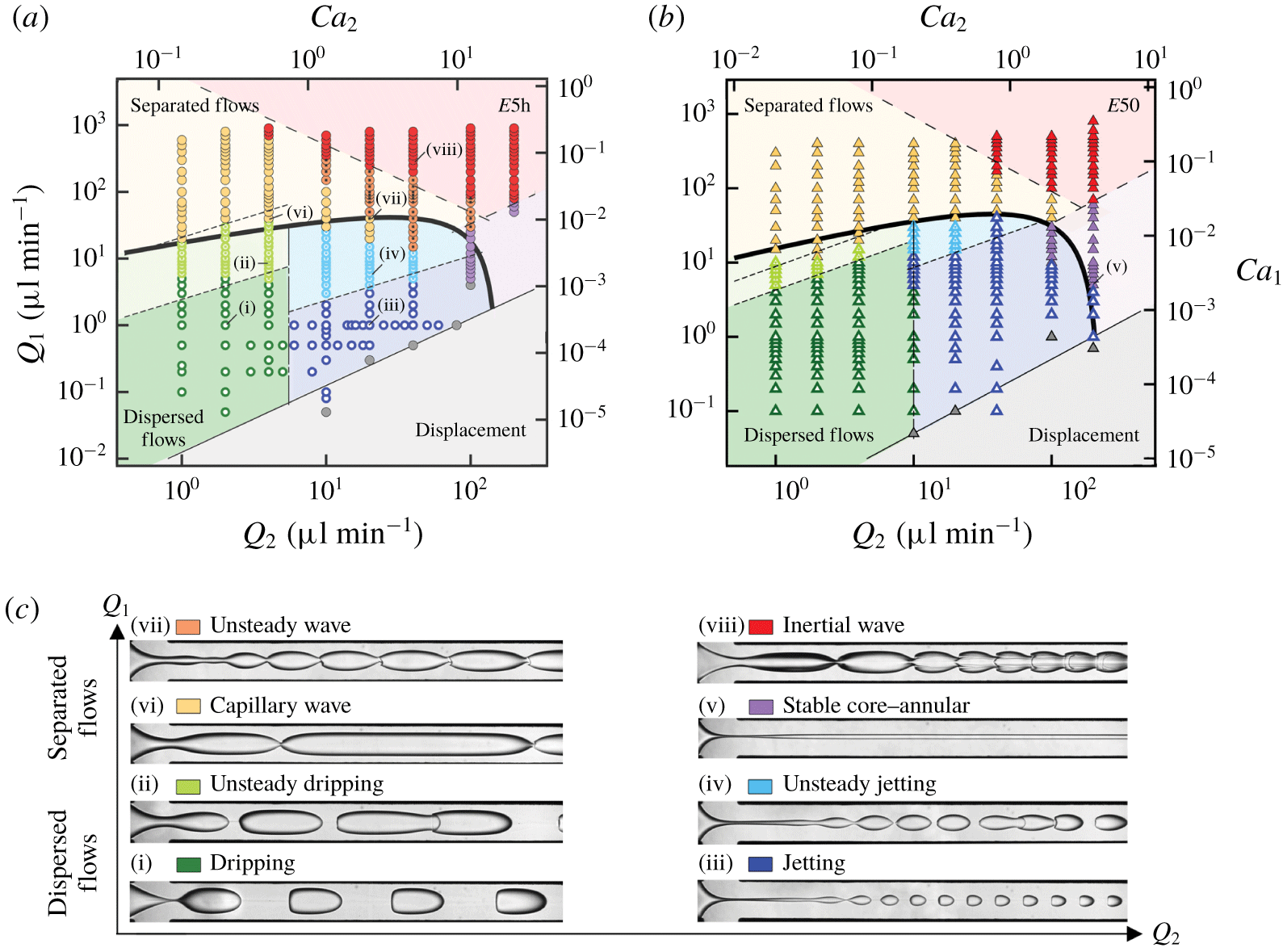
(a,b) Flow maps of fluid pairs (a)  $E5\text{h}$ and (b)
 $E50$ in terms of flow rates and capillary numbers. See main text for transition curves. (c) Experimental micrographs of flow regimes (flow rates
 $(Q_{1},~Q_{2})$ in
 $\unicode[STIX]{x03BC}\text{l}~\text{min}^{-1}$). Dispersed flows: (i) dripping (1, 2), (ii) unsteady dripping (9, 4), (iii) jetting (1, 20) and (iv) unsteady jetting (4, 20). Separated flows: (v) stable core–annular (5, 200), (vi) capillary wave (40, 4), (vii) unsteady wave (40, 20) and (viii) inertial wave (350, 40).

Two-phase flow patterns are generally classified as separated flows when both fluids form continuous streams and as dispersed flows when a phase forms discrete bubbles or droplets in the other phase. Here, separated flows correspond to wavy core–annular flows with distinct characteristics, while dripping and jetting regimes are treated as dispersed flows. Jetting patterns display intermediate features with the formation of a core–annular flow, or jet, near the junction and the emission of droplets at the tip of the jet in the observation channel. Although separated flow pattern features may further evolve downstream due to the entrainment of filamentous structures from wave crests, we restrict our analysis to relatively short distance  $x/h\sim 16$ from the junction to directly compare the initial flow characteristics between all regimes. Analysis of flow behaviour near the fluid junction is also relevant for lab-on-a-chip applications where short microfluidic elements are combined.
For a given fluid pair, variations of both central and side stream flow rates,  $Q_{1}$ and
 $Q_{2}$, grant access to a variety of flow regimes, as can be seen in figure 2. These quantities are made non-dimensional using capillary numbers such as
 $Ca_{i}=\unicode[STIX]{x1D702}_{i}J_{i}/\unicode[STIX]{x1D6FE}_{12}$, where
 $J_{i}=Q_{i}/h^{2}$ is the injection superficial velocity of fluid
 $L\mathit{i}$ (
 $i=1,2$). While the flow maps of fluid pairs
 $E5\text{h}$ and
 $E50$ show similar arrangements of flow regions, differences in the relative areas and transitions between flow regimes are apparent. Overall, separated flows are observed at large
 $Q_{1}$ and dispersed flows are found at small
 $Q_{1}$. In the droplet regimes, dripping flows with large wavelength
 $\unicode[STIX]{x1D706}$ are generated at low
 $Q_{2}$, and jetting patterns with small
 $\unicode[STIX]{x1D706}$ occur at high
 $Q_{2}$. A somewhat similar behaviour is found for separated flows, where waves of large
 $\unicode[STIX]{x1D706}$ are observed at small
 $Q_{2}$ and short waves are generated at large
 $Q_{2}$. Similar to our previous work on the development of interfacial waves in two-layer viscosity-stratified flows made of miscible or immiscible fluid pairs (Hu & Cubaud Reference Hu and Cubaud2018), we classify the long-wave regime as capillary waves and the short-wave configuration as inertial waves.
In the capillary wave regime, the wavelength  $\unicode[STIX]{x1D706}$ increases along the flow direction before stabilizing, and the inertial regime is characterized with a spatially decreasing
 $\unicode[STIX]{x1D706}$, which reaches a nearly constant value further downstream. An apparently stable core–annular flow regime is also found in the experimental field of view for intermediate values of
 $Q_{1}$ at large
 $Q_{2}$. In addition, unsteady variations of basic droplet flow patterns are located near wave regime transitions due, in particular, to a small droplet spacing
 $L$ leading to coalescence in the unsteady dripping and jetting regimes. Likewise, complex spatial variations of
 $\unicode[STIX]{x1D706}$ are observed in the unsteady wave regime between the capillary and inertial wave regimes, where the wavelength
 $\unicode[STIX]{x1D706}$ first decreases and then increases along the flow direction. Finally, a displacement regime, where the high-viscosity fluid
 $L2$ engulfs the low-viscosity fluid
 $L1$ channel resulting in no periodic pattern, is identified for very large
 $Q_{2}$ and low
 $Q_{1}$. This limiting case is found below low flow-rate ratios
 $\unicode[STIX]{x1D711}=Q_{1}/Q_{2}$, such as
 $1.25\times 10^{-2}$ for fluid pair
 $E5\text{h}$ and
 $5\times 10^{-3}$ for
 $E50$, as shown in figure 2, and presents analogies with the situation where the high-viscosity fluid is injected from the central channel of a square hydrodynamic focusing section (Cubaud & Mason Reference Cubaud and Mason2008). Other transitional lines on the flow map are discussed in following sections. In particular, we derive analytical criteria to unravel basic flow features and elucidate the transition curve between dispersed and separated flows across all regimes.
4 Dispersed flows
Dispersed flow regimes comprise both steady and unsteady dripping and jetting flow patterns. The dripping regime is obtained at low capillary numbers for small flow rates  $Q_{1}$ and
 $Q_{2}$ and is one of the most widely encountered regimes in microfluidic applications in the chemical and biological fields, where droplets are used as reaction chambers. By contrast, the jetting regime is reached at moderate capillary number and finds use to generate small droplets with applications in drug delivery. In this context, predicting the size of the droplet
 $d$ has received considerable attention in microfluidic studies (Anna Reference Anna2016). Here, we systematically examine the morphology and dynamics of droplet flows based on droplet length
 $d$, spacing
 $L$ and velocity
 $V_{D}$ for a wide range of flow rates and three different fluid pairs with a highly viscous continuous phase.
4.1 Droplet mobility
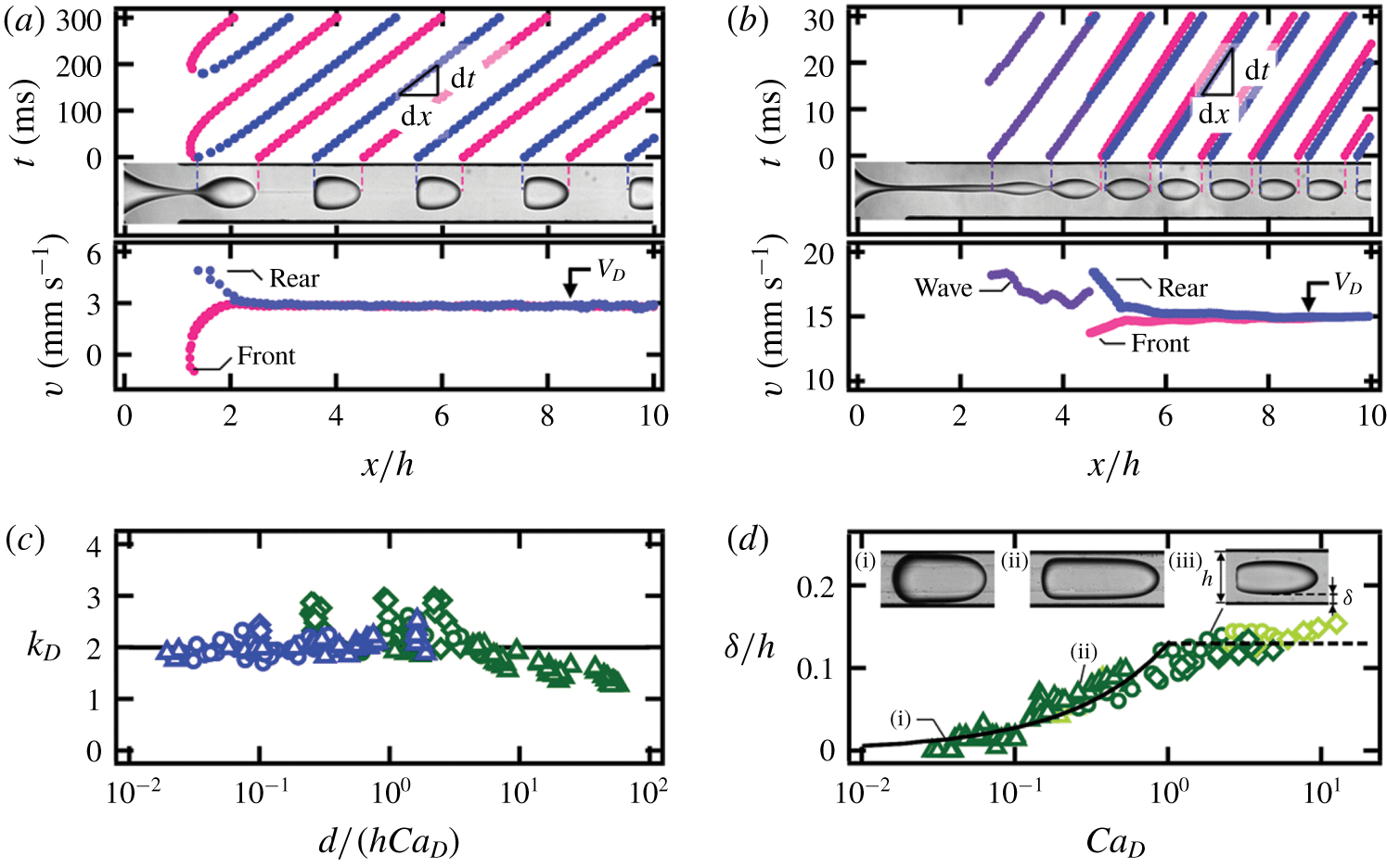
Droplet velocity and normalized film thickness. Droplet velocity  $V_{D}$ is measured on the traces for (a) dripping ((
 $Q_{1},~Q_{2}$), fluid pair)
 $=$ ((1, 4),
 $E5\text{h}$) and (b) jetting ((4, 20),
 $E5\text{h}$) flows (flow rates in
 $\unicode[STIX]{x03BC}\text{l}~\text{min}^{-1}$). (c) Evolution of droplet mobility: solid line,
 $k_{D}=2$ (
 $E50$, ▵;
 $E5\text{h}$, ○; and
 $E5\text{k}$, ♢). (d) Normalized film thickness
 $\unicode[STIX]{x1D6FF}/h$ versus droplet capillary number
 $Ca_{D}$: solid line,
 $\unicode[STIX]{x1D6FF}/h=0.13Ca_{D}^{2/3}$ (
 $Ca_{D}<1$); dashed line,
 $\unicode[STIX]{x1D6FF}/h=0.13$ (
 $Ca_{D}>1$). Inset: micrographs of deformed droplets: (i) ((0.5, 1),
 $E50$), (ii) ((5, 2),
 $E50$) and (iii) ((4, 4),
 $E5\text{h}$).

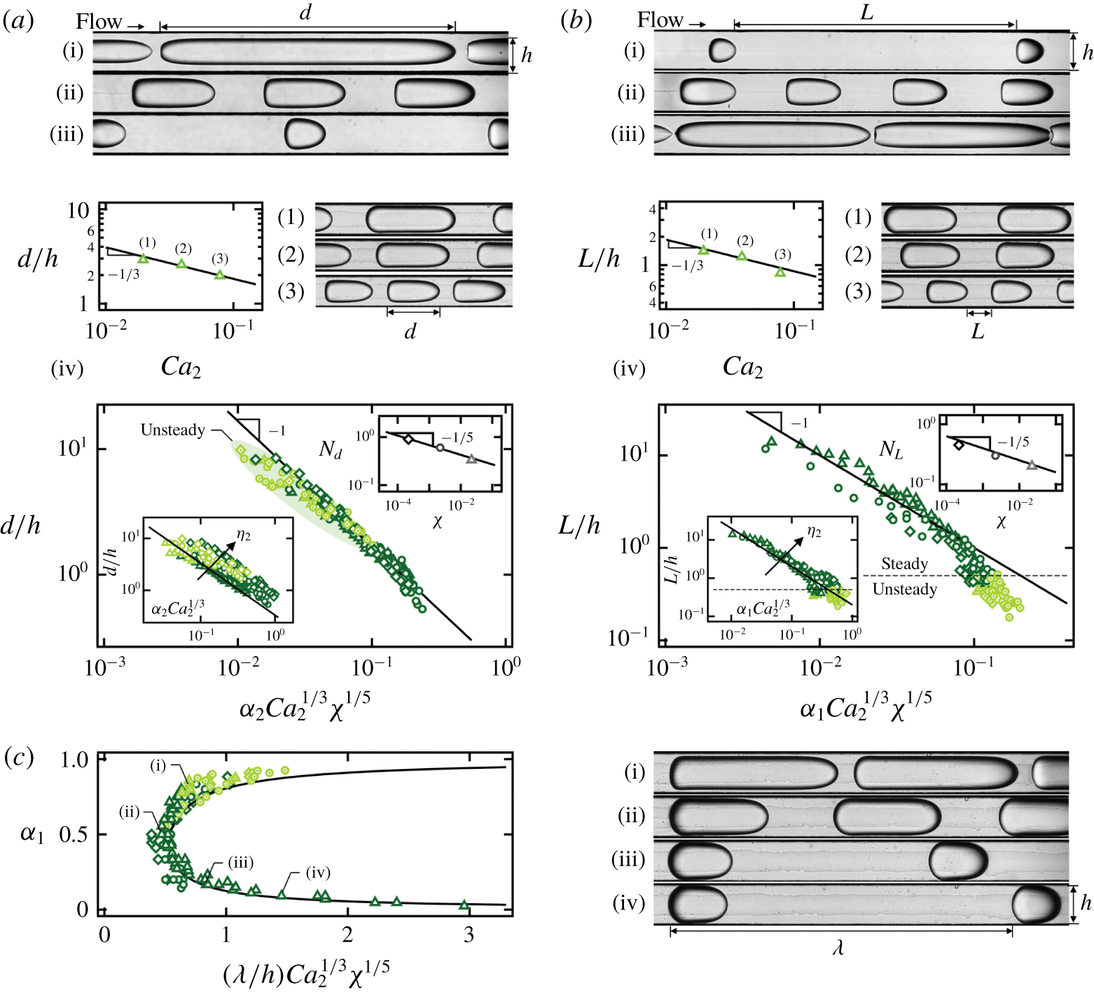
Dripping regime morphology with fluid pairs  $E50$ (▵),
 $E5\text{h}$ (○) and
 $E5\text{k}$ (♢). (a) Main graph: normalized droplet length
 $d/h$; solid line,
 $d/h=0.17(\unicode[STIX]{x1D6FC}_{2}Ca_{2}^{1/3}\unicode[STIX]{x1D712}^{1/5})^{-1}$. Bottom inset:
 $d/h$ versus
 $\unicode[STIX]{x1D6FC}_{2}Ca_{2}^{1/3}$; solid line,
 $d/h=0.33(\unicode[STIX]{x1D6FC}_{2}Ca_{2}^{1/3})^{-1}$. Top inset: correction factor; solid line,
 $N_{d}=0.17\unicode[STIX]{x1D712}^{-1/5}$. Micrographs (flow rates in
 $\unicode[STIX]{x03BC}\text{l}~\text{min}^{-1}$): (i)
 $(Q_{1},~Q_{2})=(10,~1)$, (ii) (1, 1) and (iii) (0.1, 1). (iv) Plot of
 $d/h$ versus
 $Ca_{2}$ for fixed
 $\unicode[STIX]{x1D6FC}_{2}=0.4$; solid line,
 $d/h=0.85Ca_{2}^{-1/3}$. Micrographs from (1) to (3):
 $(Q_{1},~Q_{2})=(1.5,~1)$, (3, 2) and (6, 4). (b) Normalized droplet spacing
 $L/h$; solid line,
 $L/h=0.1(\unicode[STIX]{x1D6FC}_{1}Ca_{2}^{1/3}\unicode[STIX]{x1D712}^{1/5})^{-1}$. Bottom inset:
 $L/h$ versus
 $\unicode[STIX]{x1D6FC}_{1}Ca_{2}^{1/3}$; solid line,
 $L/h=0.5(\unicode[STIX]{x1D6FC}_{1}Ca_{2}^{1/3})^{-1}$. Top inset: correction factor
 $N_{L}=0.1\unicode[STIX]{x1D712}^{-1/5}$ (solid line). Micrographs: (i)
 $(Q_{1},~Q_{2})=(0.1,~2)$, (ii) (1, 2) and (iii) (10, 2). (iv) Plot of
 $L/h$ versus
 $Ca_{2}$ for fixed
 $\unicode[STIX]{x1D6FC}_{1}=0.5$; solid line,
 $L/h=0.4Ca_{2}^{-1/3}$. Micrographs from (1) to (3):
 $(Q_{1},~Q_{2})=(1,~1)$, (2, 2) and (4, 4). (c) Rescaled dimensionless wavelength
 $(\unicode[STIX]{x1D706}/h)Ca_{2}^{1/3}\unicode[STIX]{x1D712}^{1/5}$ evolving with
 $\unicode[STIX]{x1D6FC}_{1}$; solid line,
 $(\unicode[STIX]{x1D706}/h)Ca_{2}^{1/3}\unicode[STIX]{x1D712}^{1/5}=0.17(1-\unicode[STIX]{x1D6FC}_{1})^{-1}+0.1\unicode[STIX]{x1D6FC}_{1}^{-1}$. Micrographs: (i)
 $(Q_{1},~Q_{2})=(5,~1)$, (ii) (1, 1), (iii) (0.2, 1) and (iv) (0.1, 1).

We first examine the velocity  $V_{D}$ of droplets in the dripping and jetting regimes. To measure
 $V_{D}$, spatiotemporal (
 $x$–
 $t$) diagrams are generated by tracking the front
 $x_{F}$ and rear
 $x_{R}$ positions of droplets using high-speed imaging. For steady dripping and jetting flows, the measured front and rear velocities,
 $V_{F}=\text{d}x_{F}/\text{d}t$ and
 $V_{R}=\text{d}x_{R}/\text{d}t$, of all droplets form specific curves that merge further downstream to reach a constant value
 $V_{D}$ (figure 3a,b). By contrast, for unsteady dripping and jetting flows, the spatial evolution of velocity slightly differs from droplet to droplet. For both steady and unsteady flows, the average droplet velocity
 $V_{D}$ is compared to the multi-fluid flow superficial velocity
 $J_{T}=(Q_{1}+Q_{2})/h^{2}$, such as
 $V_{D}=k_{D}J_{T}$, where
 $k_{D}$ is the droplet mobility coefficient. The coefficient of droplet mobility
 $k_{D}$ typically decreases with the droplet length
 $d$ and grows with the capillary number of the continuous phase,
 $Ca_{D}=V_{D}\unicode[STIX]{x1D702}_{2}/\unicode[STIX]{x1D6FE}_{12}$, which controls the thickness of the lubricating layer
 $\unicode[STIX]{x1D6FF}$ between droplets and walls. Measurements of
 $k_{D}$ are reported as a function of
 $d/(hCa_{D})$ for all fluid pairs in steady dripping and jetting regimes in figure 3(c) and display an average value around
 $k_{D}\approx 2$ in good agreement with the assumption that small droplets travel near the peak velocity of parabolic flows in square ducts,
 $2.1J_{T}$. Droplet mobility analysis typically includes droplet deformation, channel confinement and the presence of corner flows and lubricating films at the walls (Lac & Sherwood Reference Lac and Sherwood2009; Jakiela et al. Reference Jakiela, Makulska, Korczyk and Garstecki2011; Nath et al. Reference Nath, Biswas, Dalal and Sahu2017; Rivero-Rodriguez & Scheid Reference Rivero-Rodriguez and Scheid2018). Here, measurements show that the mobility
 $k_{D}$ is enhanced when
 $d/h$ is small and
 $Ca_{D}$ is large and data suggest that the average droplet velocity scales as
 $$\begin{eqnarray}V_{D}=2J_{T}.\end{eqnarray}$$
For confined droplets with length  $d>h$, the relationship between film thickness
 $\unicode[STIX]{x1D6FF}$ and capillary number
 $Ca$ corresponds to the classic Bretherton problem (Bretherton Reference Bretherton1961). In our square microchannels, the normalized film thickness follows the classic scaling such as
 $\unicode[STIX]{x1D6FF}/h=0.13Ca_{D}^{2/3}$ for moderate
 $Ca_{D}<1$ (figure 3d). For larger
 $Ca_{D}$, the film thickness reaches a plateau
 $\unicode[STIX]{x1D6FF}/h\approx 0.13$ similar to the case of water droplets in silicone oils with significantly larger
 $\unicode[STIX]{x1D6FE}_{12}$ (Jose & Cubaud Reference Jose and Cubaud2014). The magnitude of the prefactor in the relationship between
 $\unicode[STIX]{x1D6FF}$ and
 $Ca_{D}$ depends on flow configurations and confinement geometry (Wong, Radke & Morris Reference Wong, Radke and Morris1995; Balestra, Zhu & Gallaire Reference Balestra, Zhu and Gallaire2018). Overall, the mobility coefficient has influence on flow morphology, in particular for the wavelength
 $\unicode[STIX]{x1D706}$ of segmented flows.
4.2 Dripping
We now turn our attention to the morphology of dripping flows based on droplet length  $d$ and spacing
 $L$. In particular, we wish to predict the transition to separated flows when
 $L\rightarrow 0$ based on fluid and flow parameters. Similar to the case of bubbles, where the internal viscosity is neglected, the droplet length is estimated as
 $d=V_{D}T_{2}$, where
 $T_{2}$ is the pinching time corresponding to the filling of the junction by liquid
 $L2$,
 $T_{2}=h^{3}/Q_{2}$. Introducing the continuous-phase liquid fraction
 $\unicode[STIX]{x1D6FC}_{2}=Q_{2}/(Q_{1}+Q_{2})$ yields a scaling such as
 $d/h=k_{D}/\unicode[STIX]{x1D6FC}_{2}$ for the droplet size at low capillary numbers. At large
 $Ca$, however, the influence of viscous forces becomes significant and, for a given fluid pair, the droplet size also depends on absolute flow velocity. To measure the influence of
 $Ca$, we fix
 $\unicode[STIX]{x1D6FC}_{2}$, and measure the droplet size
 $d$ as a function of
 $Ca_{2}=\unicode[STIX]{x1D702}_{2}J_{2}/\unicode[STIX]{x1D6FE}_{12}$ to find a scaling of the form
 $d/h\sim Ca_{2}^{-1/3}$ (figure 4). While the droplet length
 $d$ scales with
 $(\unicode[STIX]{x1D6FC}_{2}Ca_{2}^{1/3})^{-1}$, systematic shifts in data points are observed based on viscosity ratio
 $\unicode[STIX]{x1D712}$, which suggests the existence of a correction factor
 $N_{d}$ associated with previous scaling. Hence, we curve-fit dimensionless droplet length
 $d/h$ as a function of
 $N_{d}(\unicode[STIX]{x1D6FC}_{2}Ca_{2}^{1/3})^{-1}$ for each fluid pair and find a weak dependence on viscosity ratio
 $N_{d}=0.17\unicode[STIX]{x1D712}^{-1/5}$ (figure 4). Finally, the normalized droplet length for all fluid pairs is shown to scale as
 $$\begin{eqnarray}d/h=a(\unicode[STIX]{x1D6FC}_{2}Ca_{2}^{1/3}\unicode[STIX]{x1D712}^{1/5})^{-1},\end{eqnarray}$$
where the constant  $a=0.17$. As expected, the unsteady dripping regime is found for large droplet length
 $d$; however, a criterion solely based on
 $d$ is not sufficient to predict regime transition, as steady and unsteady regimes are found in the same area (figure 4a).
The spacing  $L$ between droplets can be estimated using a similar argument in conjunction with mass conservation of segmented flows over a unit cell of equivalent wavelength
 $\unicode[STIX]{x1D706}=d+L$ and period
 $T$, where droplet length
 $d\sim Q_{1}T/h^{2}$ and spacing
 $L\sim Q_{2}T/h^{2}$, which leads to the scaling
 $d/L\sim Q_{1}/Q_{2}=\unicode[STIX]{x1D711}$. While a detailed discussion of the aspect ratio
 $d/L$ is presented later, the relationship
 $d/L\sim \unicode[STIX]{x1D711}$ in turn yields
 $L/h\sim (d/h)/\unicode[STIX]{x1D711}\sim (\unicode[STIX]{x1D6FC}_{1}Ca_{2}^{1/3}\unicode[STIX]{x1D712}^{1/5})^{-1}$, where
 $\unicode[STIX]{x1D6FC}_{1}=Q_{1}/(Q_{1}+Q_{2})$ is the dispersed-phase volume fraction. Similar exponents are found experimentally with
 $L/h\sim Ca_{2}^{-1/3}$ for fixed
 $\unicode[STIX]{x1D6FC}_{1}$ and correction factor
 $N_{L}=0.1\unicode[STIX]{x1D712}^{-1/5}$ for different fluid pairs. Overall, the normalized spacing experimentally follows
 $$\begin{eqnarray}L/h=b(\unicode[STIX]{x1D6FC}_{1}Ca_{2}^{1/3}\unicode[STIX]{x1D712}^{1/5})^{-1},\end{eqnarray}$$
where  $b=0.1$ (figure 4b). Data points depart from previous scaling for spacing
 $L/h<1$ and
 $\unicode[STIX]{x1D6FC}_{1}Ca_{2}^{1/3}\unicode[STIX]{x1D712}^{1/5}>0.1$ as the flow becomes concentrated and finally leads to unsteady dripping regime for
 $L/h<0.5$.
The equivalent wavelength  $\unicode[STIX]{x1D706}=d+L$ of dripping flows is therefore estimated according to
 $\unicode[STIX]{x1D706}/h\approx a(\unicode[STIX]{x1D6FC}_{2}Ca_{2}^{1/3}\unicode[STIX]{x1D712}^{1/5})^{-1}+b(\unicode[STIX]{x1D6FC}_{1}Ca_{2}^{1/3}\unicode[STIX]{x1D712}^{1/5})^{-1}$, which can be rewritten as
 $(\unicode[STIX]{x1D706}/h)Ca_{2}^{1/3}\unicode[STIX]{x1D712}^{1/5}\approx a\unicode[STIX]{x1D6FC}_{2}^{-1}+b\unicode[STIX]{x1D6FC}_{1}^{-1}=0.17(1-\unicode[STIX]{x1D6FC}_{1})^{-1}+0.1\unicode[STIX]{x1D6FC}_{1}^{-1}$. When the rescaled dimensionless wavelength
 $(\unicode[STIX]{x1D706}/h)Ca_{2}^{1/3}\unicode[STIX]{x1D712}^{1/5}$ is plotted as a function of
 $\unicode[STIX]{x1D6FC}_{1}$, the data points for the three fluid pairs collapse together and agree well with the derived formula (figure 4c). The minimum
 $\unicode[STIX]{x1D706}$ is found at
 $\unicode[STIX]{x1D6FC}_{1}=0.5$ at the transition between diluted and concentrated droplet flows. As droplets are generated at the fluid junction in the dripping regime, our work shows that segmented flows are essentially dominated by the liquid fraction with small correcting factors based on capillary number and viscosity ratio. As the side flow rate
 $Q_{2}$ increases, the capillary breakup instability becomes convected further downstream in the jetting regime.
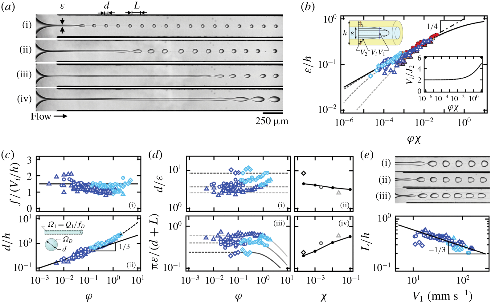
Jetting regime with fluid pairs  $E50$ (▵),
 $E5\text{h}$ (○) and
 $E5\text{k}$ (♢). (a) Micrographs of jetting streams (flow rates in
 $\unicode[STIX]{x03BC}\text{l}~\text{min}^{-1}$): (i)
 $(Q_{1},~Q_{2})=(0.1,~10)$, (ii) (0.5, 20), (iii) (1, 40) and (iv) (2, 40) (fluids
 $E5\text{h}$). (b) Inner-stream size
 $\unicode[STIX]{x1D700}/h$ as a function of
 $\unicode[STIX]{x1D711}\unicode[STIX]{x1D712}$; solid line,
 $\unicode[STIX]{x1D700}/h=(1+(\unicode[STIX]{x1D711}\unicode[STIX]{x1D712})^{-1/2})^{-1/2}$; dot-dashed line,
 $\unicode[STIX]{x1D700}/h=(\unicode[STIX]{x1D711}\unicode[STIX]{x1D712})^{1/4}$; dashed lines, equation (4.4). Top inset: schematics of velocity profile in a core–annular flow. Bottom inset:
 $V_{i}/J_{2}$ as a function of
 $\unicode[STIX]{x1D711}\unicode[STIX]{x1D712}$; solid line, equation (4.6). (c) Influence of
 $\unicode[STIX]{x1D711}$. (i) Droplet emission frequency
 $f$; solid line,
 $fh/V_{i}=1.5$. (ii) Normalized droplet length
 $d/h$; solid line,
 $d/h=\unicode[STIX]{x1D711}^{1/3}$; dashed line,
 $d/h=\unicode[STIX]{x1D711}^{1/3}+\unicode[STIX]{x1D711}/2$. (d) Comparison with linear instability analysis. (i) Plot of
 $d/\unicode[STIX]{x1D700}$ as a function of
 $\unicode[STIX]{x1D711}$ for various
 $\unicode[STIX]{x1D712}$. (ii) Average
 $d/\unicode[STIX]{x1D700}$ versus
 $\unicode[STIX]{x1D712}$; solid line, Tomotika’s theory. (iii) Mode of maximum instability
 $\unicode[STIX]{x03C0}\unicode[STIX]{x1D700}/(d+L)$ versus
 $\unicode[STIX]{x1D711}$. Average mode as a function of
 $\unicode[STIX]{x1D712}$; solid line, Tomotika’s theory. (e) Plot of
 $L/h$ versus
 $V_{1}$; solid line,
 $L/h=1.3V_{1}^{-1/3}$. Micrographs for fixed
 $\unicode[STIX]{x1D711}=0.1$: (i) ((2, 20),
 $E50$), (ii) ((1, 10),
 $E5\text{h}$) and (iii) ((0.2, 2),
 $E5\text{k}$).

4.3 Jetting
The jetting regime corresponds to droplet formation through the breakup of an initially stable central stream at a distance  $L_{S}$ from the junction. Droplets are periodically emitted from the central stream, which we label primary flow, due to the development of Rayleigh–Plateau instabilities (figure 5a). In this section, we combine periodicity and instability analysis to understand the dynamics and morphology of jetting flows.
4.3.1 Primary flow
The primary flow is modelled as a time-invariant core–annular flow without significant development of instability patterns near the fluid junction. Flow characteristics include the inner-stream diameter  $\unicode[STIX]{x1D700}$, average velocities of both inner and outer streams,
 $V_{1}$ and
 $V_{2}$, and interfacial velocity
 $V_{i}$, which depends on control parameters, including flow rates and fluid viscosities,
 $Q_{1}$,
 $Q_{2}$,
 $\unicode[STIX]{x1D702}_{1}$ and
 $\unicode[STIX]{x1D702}_{2}$. We consider a simplified one-dimensional model of core–annular flow in a circular channel, which provides a useful approximation to a compact square channel, especially when
 $\unicode[STIX]{x1D700}$ is small. Following the analysis of Cao et al. (Reference Cao, Ventresca, Sreenivas and Prasad2003) in the Stokes regime, the stream diameter
 $\unicode[STIX]{x1D700}$ is determined by the flow-rate ratio
 $\unicode[STIX]{x1D711}$ and the viscosity ratio
 $\unicode[STIX]{x1D712}$ according to
 $$\begin{eqnarray}\frac{\unicode[STIX]{x1D700}}{h}=\sqrt{\frac{1+\unicode[STIX]{x1D711}-\sqrt{1+\unicode[STIX]{x1D711}\unicode[STIX]{x1D712}^{-1}}}{2+\unicode[STIX]{x1D711}-\unicode[STIX]{x1D712}^{-1}}}.\end{eqnarray}$$
The diameter  $\unicode[STIX]{x1D700}$ allows for estimating average velocities according to
 $V_{1}=4Q_{1}/(\unicode[STIX]{x03C0}\unicode[STIX]{x1D700}^{2})$ for the inner stream and
 $V_{2}=4Q_{2}/(4h^{2}-\unicode[STIX]{x03C0}\unicode[STIX]{x1D700}^{2})$ for the outer stream. As the inner-stream diameter
 $\unicode[STIX]{x1D700}$ is seen to slightly increase along the flow direction due to entrance effects and instability development (figure 5a), the mean
 $\unicode[STIX]{x1D700}$ is measured in the middle of the stable stream at
 $x=L_{S}/2$, and the data show excellent agreement with (4.4), in particular for low values of
 $\unicode[STIX]{x1D700}$ at different
 $\unicode[STIX]{x1D712}$ (figure 5b). An asymptotic behaviour is found for low viscosity ratios
 $\unicode[STIX]{x1D712}\ll 1$ by simplifying (4.4) according to
 $$\begin{eqnarray}\unicode[STIX]{x1D700}/h=(1+(\unicode[STIX]{x1D711}\unicode[STIX]{x1D712})^{-1/2})^{-1/2},\end{eqnarray}$$
which is a function of  $\unicode[STIX]{x1D711}\unicode[STIX]{x1D712}$ only and agrees well with experimental data. Over our range of parameters, locally stable jets are observed for
 $\unicode[STIX]{x1D711}\unicode[STIX]{x1D712}\ll 1$ when (4.4) further reduces into a scaling of the form
 $\unicode[STIX]{x1D700}/h\approx (\unicode[STIX]{x1D711}\unicode[STIX]{x1D712})^{1/4}$ (figure 5b). This simple relationship provides insights into the dependence of
 $V_{1}$ on
 $Q_{1}$ and
 $Q_{2}$ as
 $V_{1}\sim 4(Q_{1}Q_{2})^{1/2}/(\unicode[STIX]{x03C0}h^{2}\unicode[STIX]{x1D712}^{1/2})$, which is proportional to the geometrical mean of injection flow rates.
An important characteristic of separated flows is the interfacial velocity  $V_{i}$. For a core–annular flow in a circular pipe, analytically solving Stokes equations yields
 $V_{i}=2V_{2}$, where
 $V_{2}=4Q_{2}/(4h^{2}-\unicode[STIX]{x03C0}\unicode[STIX]{x1D700}^{2})$ is the average velocity of the outer stream. For square channels, we approximate
 $V_{i}$ using (4.5) and obtain
 $$\begin{eqnarray}V_{i}=2[1+(4/\unicode[STIX]{x03C0}-1+4/\unicode[STIX]{x03C0}(\unicode[STIX]{x1D711}\unicode[STIX]{x1D712})^{-1/2})^{-1}]J_{2},\end{eqnarray}$$
where  $J_{2}=Q_{2}/h^{2}$. This expression is found to overlap with the exact solution of (4.4) and clearly shows that the approximation
 $V_{i}/J_{2}\approx 2$ is valid for
 $\unicode[STIX]{x1D711}\unicode[STIX]{x1D712}<0.1$ (figure 5b, bottom inset).
4.3.2 Droplet formation in jetting
Similar to a wave phenomenon, the periodic droplet emission pattern in the jetting regime is characterized by a frequency  $f$, droplet velocity
 $V_{D}$ and wavelength
 $\unicode[STIX]{x1D706}=V_{D}/f$. As droplets are generated through the breakup of the inner stream due to growing disturbances propagating along the flow direction, the droplet emission frequency
 $f$ is expected to scale as the interfacial wave frequency before breakup. Previous work on the development of capillary and inertial waves of viscosity-stratified flows (Hu & Cubaud Reference Hu and Cubaud2018) showed direct proportionality between wave frequency
 $f$ and characteristic shear rate, such as
 $f\sim V_{i}/h$. Here, we normalize
 $f$ with
 $V_{i}/h$ and probe the influence of the flow-rate ratio
 $\unicode[STIX]{x1D711}$ on the droplet emission (figure 5c (i)). For all fluid pairs, the normalized droplet emission frequency in the jetting regime remains more or less constant according to
 $$\begin{eqnarray}fh/V_{i}\approx 1.5.\end{eqnarray}$$
Information about droplet frequency  $f$ and jet diameter
 $\unicode[STIX]{x1D700}$ in turn allows for estimating the final droplet length
 $d$ using mass conservation before and after the inner-stream breakup. Balancing the equivalent droplet volume of the inner stream
 $\unicode[STIX]{x1D6FA}_{1}=Q_{1}/f$ with a spherical droplet approximation
 $\unicode[STIX]{x1D6FA}_{D}=\unicode[STIX]{x03C0}d^{3}/6$ yields normalized droplet length
 $d/h\approx [4J_{1}/(\unicode[STIX]{x03C0}V_{i})]^{1/3}=\{3/4\unicode[STIX]{x1D711}{[1+(\unicode[STIX]{x1D711}\unicode[STIX]{x1D712})^{-1/2}]^{-1}\}}^{1/3}$, which is a function of flow-rate ratio
 $\unicode[STIX]{x1D711}$ and viscosity ratio
 $\unicode[STIX]{x1D712}$ and can be simplified as
 $$\begin{eqnarray}d/h\approx \unicode[STIX]{x1D711}^{1/3}\end{eqnarray}$$
when  $\unicode[STIX]{x1D711}\unicode[STIX]{x1D712}\ll 1$. Figure 5(c)(ii) shows good agreement with experimental data for small droplets,
 $d/h<1$. A departure from the scaling relationship is observed for larger droplets
 $d/h>1$, which are typically found in the unsteady jetting regime (figure 5a (iv)). Droplets in this case become significantly deformed due to wall confinement and large capillary numbers. Overall, all data points are well fitted with an expression of the form
 $d/h=\unicode[STIX]{x1D711}^{1/3}+\unicode[STIX]{x1D711}/2$.
Therefore, for very small viscosity ratio  $\unicode[STIX]{x1D712}\ll 1$, the droplet length
 $d$ in the jetting regime does not depend on inner or outer fluid viscosities. To better understand this result, we investigate the relationship between droplet size
 $d$ and jet diameter
 $\unicode[STIX]{x1D700}$ in the light of Tomotika’s theory of Rayleigh–Plateau instability for an initially circular thread in a quiescent fluid (Tomotika Reference Tomotika1935). In particular, in the steady jetting regime, the quantity
 $d/\unicode[STIX]{x1D700}$ is found to remain fixed around a mean value that depends on the viscosity ratio
 $\unicode[STIX]{x1D712}$ (figure 5d (i)). To compare our result with linear stability analysis, we use the reported modes of maximum instability
 $x_{T}=k\unicode[STIX]{x1D700}_{T}/2$ as a function of
 $\unicode[STIX]{x1D712}$, where
 $k=2\unicode[STIX]{x03C0}/\unicode[STIX]{x1D706}_{T}$ and
 $\unicode[STIX]{x1D706}_{T}$ is the most unstable wavelength. Considering mass conservation between the jet varicose of wavelength
 $\unicode[STIX]{x1D706}_{T}$ and the resulting droplet of diameter
 $d_{T}$,
 $\unicode[STIX]{x1D706}_{T}\unicode[STIX]{x03C0}\unicode[STIX]{x1D700}^{2}/4=\unicode[STIX]{x03C0}d_{T}^{3}/6$, together with
 $\unicode[STIX]{x1D706}_{T}=\unicode[STIX]{x03C0}\unicode[STIX]{x1D700}_{T}/x_{T}$, allows us to derive the expected
 $d_{T}/\unicode[STIX]{x1D700}_{T}=[3\unicode[STIX]{x03C0}/(2x_{T})]^{1/3}$, which is a constant for each fluid pair and is compared with experimental data in figure 5(d)(ii). Deviation is observed for the fluid pair
 $E5\text{k}$, as droplets are significantly elongated along the flow direction due to the large
 $Ca$ of the outer fluid.
To circumvent the limitations associated with droplet deformation, we measure the dispersed flow wavelength  $\unicode[STIX]{x1D706}=d+L$ in figure 5(d)(iii) to directly compare experimental
 $x=\unicode[STIX]{x03C0}\unicode[STIX]{x1D700}/\unicode[STIX]{x1D706}$ and theoretical
 $x_{T}$ for each fluid pair (figure 5d (iv)) and find the agreement fairly satisfactory. It is a remarkable property of the jetting regime that the dimensionless droplet length
 $d/h\sim \unicode[STIX]{x1D711}^{1/3}$ at very small viscosity ratio
 $\unicode[STIX]{x1D712}\ll 1$ does not depend on
 $\unicode[STIX]{x1D712}$ due to the balance of the jet diameter
 $\unicode[STIX]{x1D700}$ and the mode of maximum instability of confined microjets. A somewhat equivalent property
 $d/h\sim \unicode[STIX]{x1D711}^{1/2}$ was also observed for the counterpart situation where viscosity ratio
 $\unicode[STIX]{x1D712}\gg 1$, albeit this behaviour was interpreted as a saturation of the mode of maximum instability due to thread diameter
 $\unicode[STIX]{x1D700}$ being independent of
 $\unicode[STIX]{x1D712}$ (Cubaud & Mason Reference Cubaud and Mason2008). Here, the experimental
 $\unicode[STIX]{x03C0}\unicode[STIX]{x1D700}/\unicode[STIX]{x1D706}$ is also found to remain stable in both steady and unsteady jetting regimes, as droplet length
 $d$ and spacing
 $L$ compensate one another to match the theoretical wavelength
 $\unicode[STIX]{x1D706}_{T}$. This observation highlights the importance of the viscosity ratio in the thread breakup process compared to external flow configurations. Here, we find that droplets in the jetting regime are always densely arranged with fine variations of
 $L/h<1$. Experimental data show a relationship between droplet spacing
 $L$ and the inner-stream average velocity
 $V_{1}$ according to
 $L/h\sim V_{1}^{-1/3}$ (figure 5e), suggesting that a faster inner stream leads to a shorter distance between droplets, which eventually leads to the formation of a continuous stream in the separated flow region.
4.4 Aspect ratio of dispersed flows
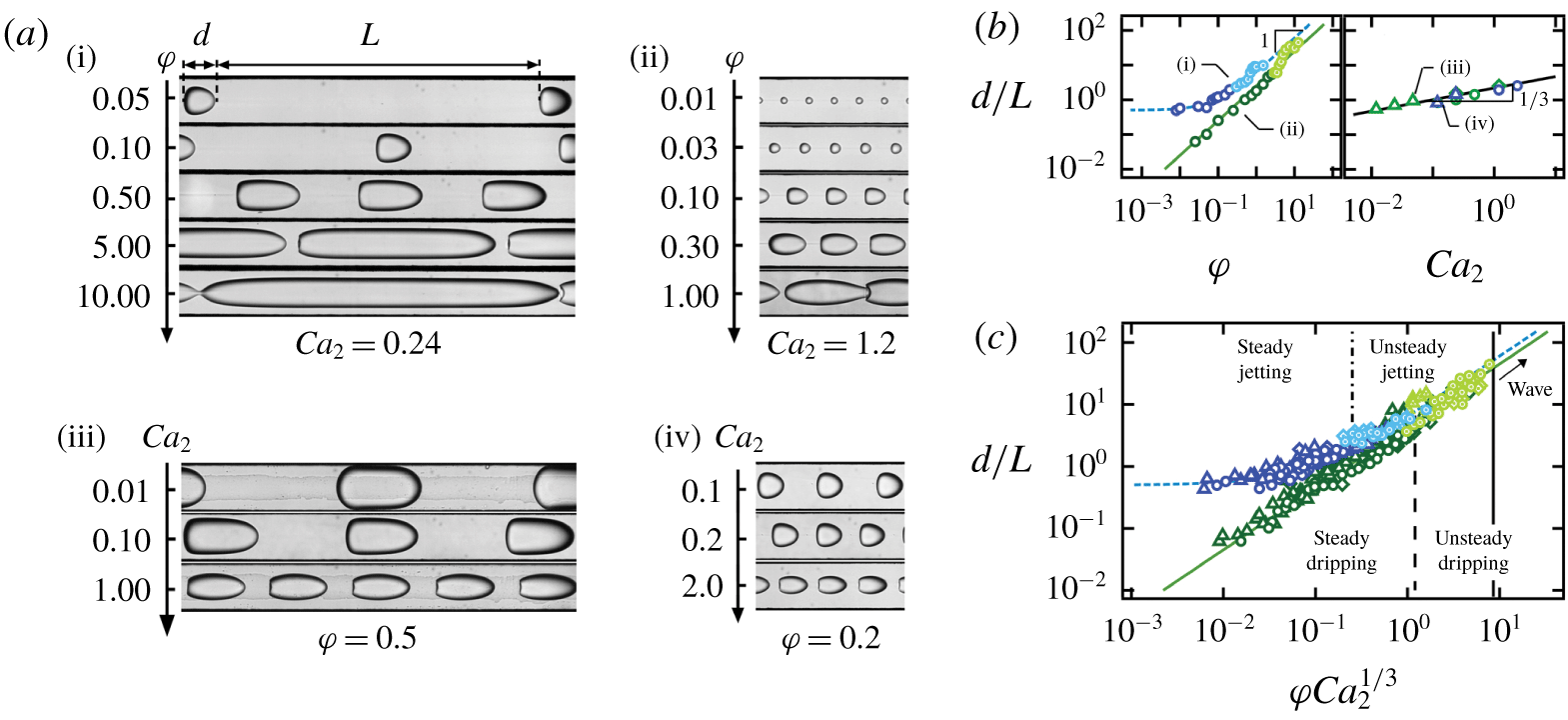
Aspect ratio of dripping and jetting regimes for fluid pairs  $E50$ (▵),
 $E5\text{h}$ (○) and
 $E5\text{k}$ (♢). (a) Micrographs of dispersed flows with various
 $d/L$ for (i) dripping with
 $Ca_{2}=0.24$, (ii) jetting for
 $Ca_{2}=1.2$, (iii) dripping with
 $\unicode[STIX]{x1D711}=0.5$ and (iv) jetting with
 $\unicode[STIX]{x1D711}=0.2$. (b) Influence of
 $\unicode[STIX]{x1D711}$ and
 $Ca_{2}$ on aspect ratio
 $d/L$ for cases shown in (a). (c) Evolution of
 $d/L$ as a function of
 $\unicode[STIX]{x1D711}Ca_{2}^{1/3}$ for all cases; solid line,
 $d/L=4.5\unicode[STIX]{x1D711}Ca_{2}^{1/3}$; dashed line,
 $d/L=0.5+4.5\unicode[STIX]{x1D711}Ca_{2}^{1/3}$.

While dripping and jetting flows display specific behaviours, both regimes transition to separated flows when  $L\rightarrow 0$, and the linear aspect ratio
 $d/L$ provides a useful method to characterize a wide range of segmented flows (figure 6a). Using continuity applied to a one-dimensional model of a repetitive unit of dispersed flows of length
 $\unicode[STIX]{x1D706}$ over a period
 $T$, such as
 $dh^{2}\sim Q_{1}T$ and
 $Lh^{2}\sim Q_{2}T$, yields the simple relationship
 $d/L\sim \unicode[STIX]{x1D711}$, which accurately represents the behaviour of dripping flows as well as jetting flows when
 $d>h$ (figure 6b (i)). However, similar to our previous discussion of
 $d/h$ and
 $L/h$, while flow-rate ratio
 $\unicode[STIX]{x1D711}$ captures the major role of the relative flow rates (figure 6a (i,ii)), absolute flow rates also play a minor role in the morphology of dispersed flows as shown in figure 6(a)(iii,iv) with a visualization of flow patterns having similar
 $\unicode[STIX]{x1D711}$ but various
 $Ca_{2}$. To capture the influence of
 $Ca_{2}$, we plot the aspect ratio
 $d/L$ as a function of
 $Ca_{2}$ for experiments having the same flow-rate ratio
 $\unicode[STIX]{x1D711}$ and find a relationship of the form
 $d/L\sim Ca_{2}^{1/3}$ (figure 6b (ii)). Finally, the parameter
 $\unicode[STIX]{x1D711}Ca_{2}^{1/3}$ permits rescaling of dripping flows according to
 $$\begin{eqnarray}(d/L)_{\mathit{dripping}}=4.5\unicode[STIX]{x1D711}Ca_{2}^{1/3}.\end{eqnarray}$$
In contrast to the dripping regime, where  $d/L$ can be as small as
 $10^{-1}$, the ratio
 $d/L$ in the jetting regime saturates at a constant value of around 0.5 for
 $\unicode[STIX]{x1D711}Ca_{2}^{1/3}\ll 1$. This behaviour is expected since
 $d/L=d/(\unicode[STIX]{x1D706}-d)$ and both
 $d/\unicode[STIX]{x1D700}$ and
 $\unicode[STIX]{x1D706}/\unicode[STIX]{x1D700}$ are fixed for each fluid pair. Overall,
 $d/L$ in the jetting regime can be represented with the following formula:
 $$\begin{eqnarray}(d/L)_{\mathit{jetting}}=0.5+4.5\unicode[STIX]{x1D711}Ca_{2}^{1/3}.\end{eqnarray}$$
For relatively large flow-rate ratio  $\unicode[STIX]{x1D711}$, jetting data points align with the dripping curve, suggesting similar flow morphology despite widely different droplet generation mechanisms (figure 6c).
The parameter  $\unicode[STIX]{x1D711}Ca_{2}^{1/3}$ can also serve as an estimation of the transition from steady to unsteady dripping and jetting regimes, as well as to wave regimes as indicated with dashed lines on figure 2. The critical value of
 $\unicode[STIX]{x1D711}Ca_{2}^{1/3}$ for flow transition slightly vary for each fluid pair, whilst it remains of the same order of magnitude. A universal criterion for the transition between dispersed and separated flows, however, is still missing, as the condition
 $(d/L)\rightarrow \infty$ is not sufficient to predict flow regimes. In the following section, we examine the peculiar behaviour of separated flows and wave regimes, and we develop an original method to delineate multiphase flow patterns in microchannels.
5 Separated flows
5.1 Capillary and inertial waves
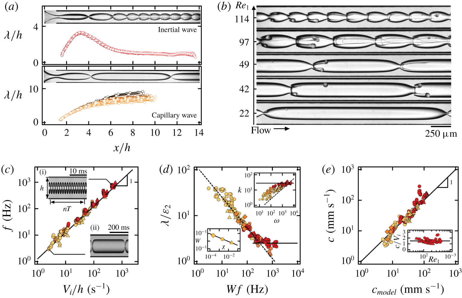
Separated flow regimes consist of stable and wavy core–annular flows with a rich collection of flow morphologies. Two main types of waves are identified: (i) inertial waves, whose wavelengths  $\unicode[STIX]{x1D706}$ reach a maximum value near the fluid junction and then decrease along the flow direction, and (ii) capillary waves, where
 $\unicode[STIX]{x1D706}$ monotonically increases along the flow direction and saturates at a relatively large value further downstream (figure 7a). The characteristic wavelength
 $\unicode[STIX]{x1D706}/h$ of each experiment is measured at the plateau region downstream at around
 $x/h\sim 10$ for both types of waves. Increasing the inner-stream Reynolds number
 $Re_{1}=\unicode[STIX]{x1D70C}_{1}V_{1}h/\unicode[STIX]{x1D702}_{1}$ allows us to examine the cross-over between wave regimes with
 $\unicode[STIX]{x1D706}/h$ ranging from 1 to 10 (figure 7b).
Another important parameter is the wave emission frequency  $f$, which is measured from spatiotemporal diagrams with
 $f=1/T$, where
 $T$ is the wave time period that is averaged over multiple cycles
 $T=t/n$ (figure 7c). Similar to our previous work on two-layer viscous stratifications (Hu & Cubaud Reference Hu and Cubaud2018), the wave frequency
 $f$ is related to the interfacial velocity
 $V_{i}$ of the primary flow, i.e. stable core–annular flow, and direct proportionality between
 $f$ and
 $V_{i}$ is recovered for both capillary and inertial waves such as
 $$\begin{eqnarray}f=1.5V_{i}/h.\end{eqnarray}$$
This relationship is identical to that of the jetting regime for the droplet emission frequency and provides insights into the connection between wave and droplet flows.
Characteristics of wave regimes. (a) Wavelength of capillary wave and inertial wave is measured downstream. (b) Evolution from capillary wave to inertial wave as  $Re_{1}$ increases. (c) Wave emission frequency
 $f=1.5V_{i}/h$. Insets: spatiotemporal diagrams. (d) Evolution of wave aspect ratio
 $\unicode[STIX]{x1D706}/\unicode[STIX]{x1D700}_{2}$ as a function of
 $Wf$; solid line,
 $\unicode[STIX]{x1D706}/\unicode[STIX]{x1D700}_{2}=2.5$. Top inset: capillary wave dispersion relationship
 $k=[(\unicode[STIX]{x1D70C}_{1}+\unicode[STIX]{x1D70C}_{2})/\unicode[STIX]{x1D6FE}_{12}]^{1/3}\unicode[STIX]{x1D714}^{2/3}$ (dashed line) and
 $k=20~\text{mm}^{-1}$ (solid line). Bottom inset: viscosity ratio coefficient
 $W=0.085\unicode[STIX]{x1D712}^{-1/2}$ (solid line). (e) Wave celerity calculated according to (5.4) agrees well with experimental results. Bottom inset: inertial waves show
 $c/V_{i}=1.5$ over a wide range of
 $Re_{1}$.

A common approach to study the time–space correlation of propagating waves is to examine the dispersion relationship such as  $D(k,\unicode[STIX]{x1D714})=0$, where
 $k=2\unicode[STIX]{x03C0}/\unicode[STIX]{x1D706}$ is the wavenumber that measures the wave spatial extension and
 $\unicode[STIX]{x1D714}=2\unicode[STIX]{x03C0}f$ is the angular frequency that characterizes temporal periodicity. Therefore, we investigate the dispersion relationship of confined capillary waves in viscous liquid–liquid systems by plotting wavenumber
 $k$ as a function of angular frequency
 $\unicode[STIX]{x1D714}$ for all three fluid pairs. In general, data points follow the typical dispersion relationship derived for capillary waves propagating at a flat interface, such as
 $k=[(\unicode[STIX]{x1D70C}_{1}+\unicode[STIX]{x1D70C}_{2})/\unicode[STIX]{x1D6FE}_{12}]^{1/3}\unicode[STIX]{x1D714}^{2/3}$ (figure 7d, top inset), with good agreement for the coefficient
 $[(\unicode[STIX]{x1D70C}_{1}+\unicode[STIX]{x1D70C}_{2})/\unicode[STIX]{x1D6FE}_{12}]^{1/3}\approx 0.12~\text{mm}^{-1}~\text{s}^{2/3}$ and the exponent
 $2/3$ associated with
 $\unicode[STIX]{x1D714}$. As we suspect data scattering due to various viscosity ratios
 $\unicode[STIX]{x1D712}$ and interfacial curvatures
 $2/\unicode[STIX]{x1D700}$, we rewrite the dispersion relationship as
 $\unicode[STIX]{x1D706}=[2\unicode[STIX]{x03C0}\unicode[STIX]{x1D6FE}_{12}/(\unicode[STIX]{x1D70C}_{1}+\unicode[STIX]{x1D70C}_{2})]^{1/3}f^{-2/3}$ using wavelength
 $\unicode[STIX]{x1D706}$ and frequency
 $f$ directly and introduce the dimensionless viscous layer of thickness
 $\unicode[STIX]{x1D700}_{2}/h=(1-\unicode[STIX]{x1D700})/(2h)$ to consider the evolution of the dimensionless wavelength as
 $\unicode[STIX]{x1D706}/\unicode[STIX]{x1D700}_{2}$, by analogy with shallow-water waves. We then plot
 $\unicode[STIX]{x1D706}/\unicode[STIX]{x1D700}_{2}$ as a function of
 $f$ and fit data according to
 $\unicode[STIX]{x1D706}/\unicode[STIX]{x1D700}_{2}=2[2\unicode[STIX]{x03C0}\unicode[STIX]{x1D6FE}_{12}/(\unicode[STIX]{x1D70C}_{1}+\unicode[STIX]{x1D70C}_{2})]^{1/3}(Wf)^{-2/3}/h$, where the coefficient
 $W=0.085\unicode[STIX]{x1D712}^{-1/2}$ depends on the viscosity ratio
 $\unicode[STIX]{x1D712}$ (figure 7d, bottom inset). Overall, the experimental results collapse onto a single curve defined with a modified dispersion relationship that reads
 $$\begin{eqnarray}\unicode[STIX]{x1D706}/\unicode[STIX]{x1D700}_{2}=2[2\unicode[STIX]{x03C0}\unicode[STIX]{x1D6FE}_{12}/(\unicode[STIX]{x1D70C}_{1}+\unicode[STIX]{x1D70C}_{2})]^{1/3}(0.085\unicode[STIX]{x1D712}^{-1/2}f)^{-2/3}/h,\end{eqnarray}$$
and can be approximated with  $\unicode[STIX]{x1D706}/\unicode[STIX]{x1D700}_{2}\approx 10.4h^{-1}[2\unicode[STIX]{x03C0}\unicode[STIX]{x1D712}\unicode[STIX]{x1D6FE}_{12}/(\unicode[STIX]{x1D70C}_{1}+\unicode[STIX]{x1D70C}_{2})]^{1/3}f^{-2/3}$. This relationship indicates the decrease of wavelength
 $\unicode[STIX]{x1D706}$ as the frequency
 $f$ grows in the capillary regime. Eventually, for large frequencies, the normalized wavelength
 $\unicode[STIX]{x1D706}/\unicode[STIX]{x1D700}_{2}$ reaches the plateau associated with inertial waves according to
 $$\begin{eqnarray}\unicode[STIX]{x1D706}/\unicode[STIX]{x1D700}_{2}=2.5.\end{eqnarray}$$
The modified dispersion relationship is used to derive the wave propagation celerity  $c_{\mathit{model}}$ as a function of control parameters according to the basic wave equation
 $c=\unicode[STIX]{x1D706}f$ such as
 $$\begin{eqnarray}c_{\mathit{model}}\approx 12\left[\frac{2\unicode[STIX]{x03C0}\unicode[STIX]{x1D712}\unicode[STIX]{x1D6FE}_{12}}{(\unicode[STIX]{x1D70C}_{1}+\unicode[STIX]{x1D70C}_{2})h}\right]^{1/3}\frac{1-\unicode[STIX]{x1D700}^{\ast }}{(4-\unicode[STIX]{x03C0}\unicode[STIX]{x1D700}^{\ast 2})^{1/3}}J_{2}^{1/3},\end{eqnarray}$$
where  $\unicode[STIX]{x1D700}^{\ast }=\unicode[STIX]{x1D700}/h$ is the dimensionless inner-stream diameter. To measure the experimental wave celerity, we digitally track the motion of wave crests using image processing. The spatial evolution of
 $c(x)$ is relatively similar to
 $\unicode[STIX]{x1D706}(x)$ and reaches a constant value in the observation channel. Overall, a good agreement is found between measured celerity
 $c$ and
 $c_{\mathit{model}}$ derived by (5.4) (figure 7e). In addition, a simplified celerity model can also be written for
 $W=1$ as
 $c_{\mathit{CAP}}=2\{3\unicode[STIX]{x03C0}\unicode[STIX]{x1D6FE}_{12}/[(\unicode[STIX]{x1D70C}_{1}+\unicode[STIX]{x1D70C}_{2})h]\}^{1/3}(1-\unicode[STIX]{x1D700}^{\ast })(4-\unicode[STIX]{x03C0}\unicode[STIX]{x1D700}^{\ast 2})^{-1/3}J_{2}^{1/3}$. For inertial waves, we find that the celerity is comparable with interfacial velocity as
 $c/V_{i}\approx 1.5$ over a wide range of
 $Re_{1}$ (figure 7e, inset).
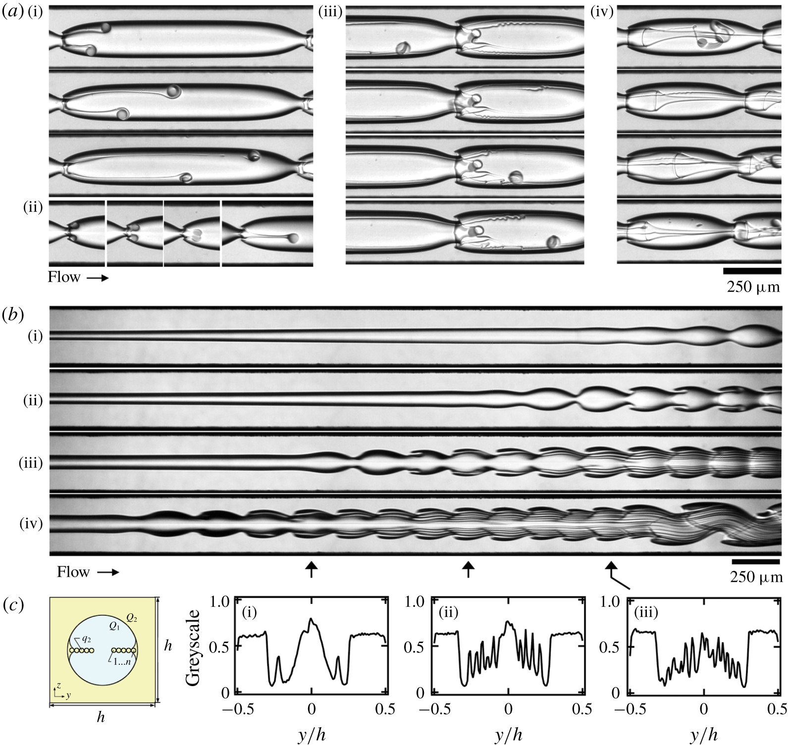
Viscous ligaments due to wave breaking. (a) Formation process of ligaments with rolling tips: (i) a pair of ligaments (( $Q_{1},~Q_{2}$), fluid pair,
 $\unicode[STIX]{x0394}t$)
 $=$ ((100, 10),
 $E5\text{h}$, 10 ms); (ii) merging ligaments ((70, 4),
 $E5\text{h}$, 14 ms); (iii) viscous bag ((150, 20),
 $E5\text{h}$, 10 ms); and (iv) transport of detached viscous tip through a neck, ((250, 10),
 $E5\text{h}$, 1 ms). (b) Ligament threads: flow rates of (i)–(iv) are
 $Q_{1}=70$, 150, 300 and 600, respectively, and
 $Q_{2}=200$,
 $E50$. (c) Schematic of ligament arrangement in cross-section view: (i)–(iii) normalized grey-scale of cross-flow direction, where local peaks represent ligaments.

5.2 Wave breaking
Interfacial viscous waves evolve and typically break with the entrainment of viscous filamentous structures from wave crests. While ligament formation and subsequent droplet generation are widely encountered in industrial and natural fragmentation processes, including spray formation (Marmottant & Villermaux Reference Marmottant and Villermaux2004) and droplet splash (Wang & Bourouiba Reference Wang and Bourouiba2018), less is known about the extrusion of viscous filaments in confined microsystems. Here, we discuss two types of ligament formation: rolling in the capillary regime, and shearing in the inertial regime (figure 8). Both of these processes result from the large shear force exerted by the fast inner stream on wave crests and the local wave structure that depends on wavelength  $\unicode[STIX]{x1D706}$.
The rolling ligament process (figure 8a (i)) is mainly observed for long waves with wavelength  $\unicode[STIX]{x1D706}\gg h$ in the capillary regime and corresponds to the emission of a rolling tip which grows into a rotating droplet connected to the wave crest with a viscous thread. The rolling behaviour is induced by the viscous torque resulting from the parabolic velocity profile of the inner stream in the flow cells. As droplets migrate towards the wave trough, their velocity remains in slight excess of the wave celerity while the connected thread wraps around the droplets. Droplets eventually break from their ‘umbilical cords’, supplying viscous material for growth through a complex thread thinning process. When the neck is narrow and a pair of ligaments are phase-locked, filaments can merge into a single ligament that travels near the centreline of the core–annular flow (figure 8a (ii)). Intriguing viscous bag formation mechanisms are also observed, where a rim of viscous material grows into a thin tubular shell. The viscous bag quickly destabilizes and interacts with ligaments and droplets further downstream (figure 8a (iii,iv)).
In the inertial regime, the breaking of short waves with wavelength  $\unicode[STIX]{x1D706}\sim h$ is characterized by the regular detachment of continuous streams of viscous material from the wave crest. In contrast to the capillary regime, filaments remain aligned with the wave crest due to the inertia associated with the fast inner stream and the tip velocity is much larger than the wave celerity. In practice, multiple ligament formation is enhanced by increasing the inner-stream flow rate as shown in figure 8(b). An important quantity of high-viscosity fluid is convected through filament detachment, resulting in the spatial depletion of the outer viscous layer with a progressive migration of the wave crest towards the walls. This process produces the self-alignment of ligaments, where newborn ligaments are always located closer to the centreline. Three cross-section grey-scale profiles are included in figure 8(c) at different locations to document the regular increase of the number of ligaments along the flow direction. Such highly complex flow structures can also experience secondary destabilization processes with the coalescence of waves further downstream.
6 Comparison and transition
6.1 Initial stable length
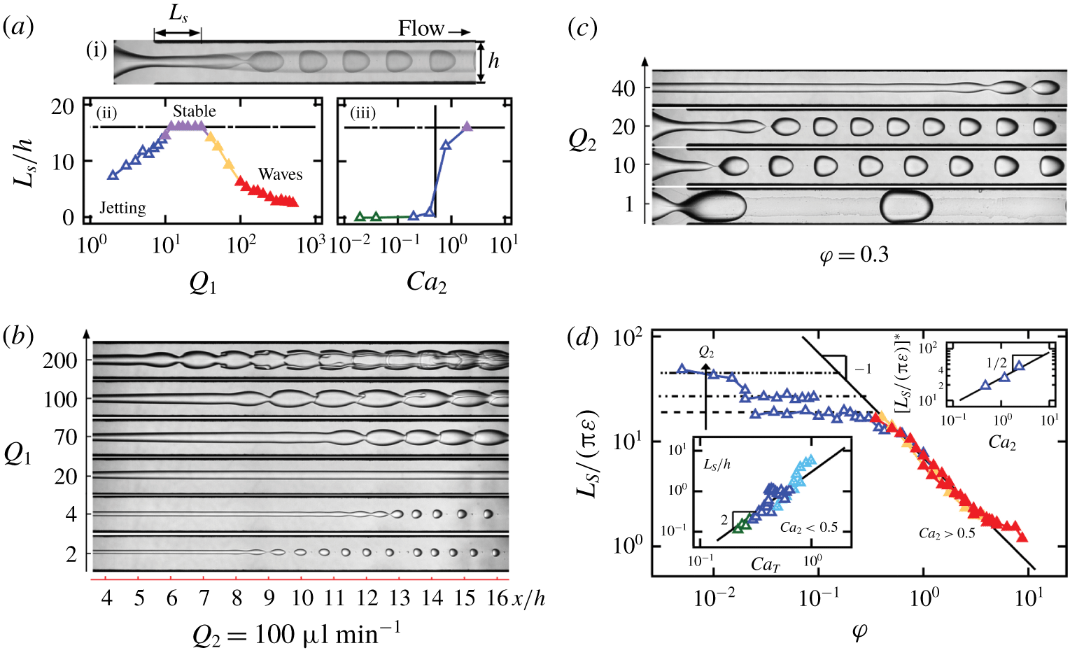
The evolution of the stable length  $L_{S}$ of core–annular flows with flow rate provides useful information about flow regimes and transitions between dripping, jetting and wavy flow patterns. To measure the average length
 $L_{S}$ for a given set of control parameters, we superpose approximately 200 frames of a high-speed video to produce a composite image and visualize the average envelope of flow to measure the length of the invariant inner stream (figure 9a (i)). While the length
 $L_{S}\sim 0$ remains constant in the dripping regime,
 $L_{S}$ increases with flow velocity in the jetting regime and decreases with flow rate in the wave regimes.
To illustrate this behaviour, we plot normalized initial stable length  $L_{S}/h$ as a function of inner-stream flow rate
 $Q_{1}$ for fixed outer-stream flow rate
 $Q_{2}$ on figure 9(a)(i), which corresponds to the flow patterns shown on figure 9(b). The length
 $L_{S}$ monotonically increases with
 $Q_{1}$ in the jetting regime until no disturbance can be observed in the field of view, i.e. for
 $L_{S}/h>16$, which corresponds to the stable core–annular flow in this study. Further increase of
 $Q_{1}$ leads to the wave regime, where
 $L_{S}$ decreases with flow rates of injection. Such non-monotonic variation of
 $L_{S}$ is also observed in open jets as flows evolve from dispersed to continuous regimes (Brennen Reference Brennen2005). To clarify the role of the inner-stream diameter
 $\unicode[STIX]{x1D700}$ in the stable length
 $L_{S}$, a similar analysis is conducted on figure 9(a)(iii) for flows having a fixed
 $\unicode[STIX]{x1D711}$ but various absolute flow rates as shown in figure 9(c). In the dripping regime, the initial length
 $L_{S}\sim 0$ at small flow rates, while for moderate flow rates,
 $L_{S}$ sharply increases in the jetting regime, in particular above a critical value of outer-stream capillary number
 $Ca_{2}\sim 0.5$, which is in good agreement with previous studies in capillary tubes (Utada et al. Reference Utada, Fernandez-Nieves, Gordillo and Weitz2008).
The presence of a critical value  $Ca_{2}$ for the large growth of
 $L_{S}$ suggests a distinction between slow flows, where
 $L_{S}$ is independent of
 $\unicode[STIX]{x1D700}$ and follows a scaling of the total capillary number
 $Ca_{T}$ as
 $L_{S}/h\approx 3Ca_{T}^{2}$ (figure 9d, bottom inset), and fast flows, where the stable length normalized with the jet circumference
 $L_{S}/(\unicode[STIX]{x03C0}\unicode[STIX]{x1D700})$ depends on
 $Ca_{2}$ according to
 $L_{S}/(\unicode[STIX]{x03C0}\unicode[STIX]{x1D700})=27Ca_{2}^{1/2}$ (figure 9d, top inset), in the jetting regime and collapse onto a master curve defined as
 $L_{S}/(\unicode[STIX]{x03C0}\unicode[STIX]{x1D700})=7/\unicode[STIX]{x1D711}$ in the wave regimes (figure 9d). A similar behaviour was observed for the development on inertial waves in miscible viscous-stratified microflows (Hu & Cubaud Reference Hu and Cubaud2016). In practice, we find that the initial stable length
 $L_{S}$ growths with flow rates for convective instabilities and decreases with flow velocities for absolute instabilities. Further theoretical and numerical work would provide more insights on the dependence of
 $L_{S}$ with control parameters. Better understanding the role of the stable length is important for hydrodynamic control of flow instabilities in microfluidic systems.
Initial length  $L_{S}$ for fluid pair
 $E50$. (a)(i) How
 $L_{S}$ is measured from image processing. (ii) Non-monotonic evolution of
 $L_{S}/h$ is observed for fixed
 $Q_{2}=100~\unicode[STIX]{x03BC}\text{l}~\text{min}^{-1}$ and various
 $Q_{1}$. (b) Micrographs corresponding to (a). (c) Normalized
 $L_{S}/h$ shows a sudden increase when
 $Ca_{2}>0.5$ for fixed
 $\unicode[STIX]{x1D711}=0.3$. (d) Dimensionless initial length
 $L_{S}/(\unicode[STIX]{x03C0}\unicode[STIX]{x1D700})$ for wave regime follows
 $L_{S}/(\unicode[STIX]{x03C0}\unicode[STIX]{x1D700})=7/\unicode[STIX]{x1D711}$ (solid line), while jetting regime with
 $Ca_{2}>0.5$ follows
 $L_{S}/(\unicode[STIX]{x03C0}\unicode[STIX]{x1D700})=27Ca_{2}^{1/2}$, as shown in top inset. Bottom inset: jetting regime for
 $Ca_{2}<0.5$ and
 $L_{S}/h=3Ca_{T}^{2}$ (solid line).

6.2 Periodicity of all regimes
In this section, we combine the periodic pattern description of dripping and jetting flows with capillary and inertial wave regimes. We discuss, in particular, the evolution of quantities such as pattern frequency  $f$, wavelength
 $\unicode[STIX]{x1D706}$ and velocity
 $V$ across all flow regimes.
6.2.1 Temporal and spatial periodicity – frequency and wavelength
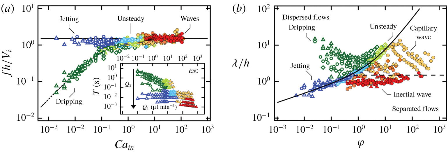
We first examine the pattern formation frequency  $f$ of dispersed and wave flow regimes. For a given fluid pair, we present the evolution of the time period
 $T=1/f$ where each curve represents experiments conducted at fixed outer-stream flow rate
 $Q_{2}$ and varying inner-stream flow rate
 $Q_{1}$ (figure 10a (inset)). It is evident from this graph that (a) the inner-stream flow rate
 $Q_{1}$ does not significantly influence the period
 $T$ of jetting and wave regimes but reduces the period
 $T$ of dripping flows, and (b) the outer-stream flow rate
 $Q_{2}$ decreases the period for all regimes, suggesting that
 $Q_{2}$ sets the level of
 $T$ in general. These observations are consistent with our previous analysis of jetting and wave emission frequencies, where
 $f\approx 1.5V_{i}/h$, with
 $V_{i}/h$ being largely determined by
 $Q_{2}$. Therefore, we use this reference and display the normalized frequency
 $fh/V_{i}$ as a function of the injection capillary number
 $Ca_{\mathit{in}}=J_{1}\unicode[STIX]{x1D702}_{2}/\unicode[STIX]{x1D6FE}_{12}$, where
 $J_{1}=Q_{1}/h^{2}$, for all fluid pairs across all regimes in figure 10(a). As expected, the data for the jetting and wave regimes collapse onto the curve
 $fh/V_{i}=1.5$. In contrast, the dripping regime features a smaller dimensionless frequency
 $f$ that is curve-fitted with
 $$\begin{eqnarray}fh/V_{i}=1.5(1+0.25Ca_{\mathit{in}}^{-3/4})^{-1},\end{eqnarray}$$
which reaches a plateau of approximately 1.5 when  $Ca_{\mathit{in}}>1$. The upper limit of the dripping frequency is therefore given by
 $f\approx 1.5V_{i}/h$, which is independent of interfacial tension but influenced by flow rates and fluid viscosities. Remarkably, the unsteady dripping and jetting regimes are observed in the same region when the two branches of steady dripping and jetting merge at the transition into wave regimes.
Frequency and wavelength of dripping, jetting and wave regimes for fluid pairs  $E50$ (▵),
 $E5\text{h}$ (○) and
 $E5\text{k}$ (♢). (a) Normalized frequency
 $fh/V_{i}$ as a function of
 $Ca_{\mathit{in}}$: solid line,
 $fh/V_{i}=1.5$; dashed line,
 $fh/V_{i}=1.5(1+0.25Ca_{\mathit{in}}^{-3/4})^{-1}$. Inset: evolution of
 $T$ with
 $Q_{1}$ as
 $Q_{2}$ is varied, fluid pair
 $E50$. (b) Normalized wavelength
 $\unicode[STIX]{x1D706}/h$ as a function of
 $\unicode[STIX]{x1D711}$: solid line,
 $\unicode[STIX]{x1D706}/h=1.5(\unicode[STIX]{x1D711}^{1/4}+\unicode[STIX]{x1D711}/3)$; dashed line,
 $\unicode[STIX]{x1D706}/h=1.5$.

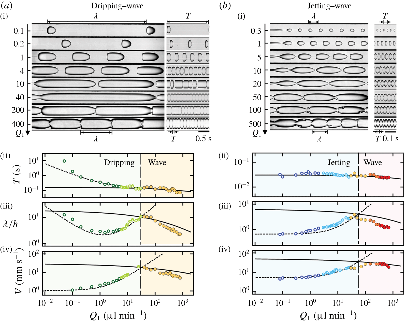
Evolution of pattern characteristics for dispersed to separated regimes,  $E5\text{h}$ (flow rates in
 $\unicode[STIX]{x03BC}\text{l}~\text{min}^{-1}$). (a) Evolution from dripping to wave regimes with fixed
 $Q_{2}=2$. (i) Micrographs and corresponding spatiotemporal diagrams at fixed
 $Q_{2}$ for varying
 $Q_{1}$. Influence of
 $Q_{1}$ on (ii) period
 $T$, (iii) wavelength
 $\unicode[STIX]{x1D706}/h$ and (iv) propagation velocity
 $V$. Critical
 $Q_{1}=30$ for dripping–wave transition. (b) Evolution from jetting to wave regime with fixed
 $Q_{2}=10$. (i) Micrographs and corresponding spatiotemporal diagrams at fixed
 $Q_{2}$ for varying
 $Q_{1}$. Influence of
 $Q_{1}$ on (ii) period
 $T$, (iii) wavelength
 $\unicode[STIX]{x1D706}/h$ and (iv) propagation velocity
 $V$. Critical
 $Q_{1}=55$ for jetting–wave transition.

The connection between dispersed and separated flows is also apparent when the periodic pattern wavelength  $\unicode[STIX]{x1D706}$ is displayed as a function of the flow-rate ratio
 $\unicode[STIX]{x1D711}$ (figure 10b). Regions of steady dripping and wave pattern data are clearly separated by a curve defined with the collapse of jetting and unsteady dripping data points. Hence, the jetting flow regime, which displays intermediate properties between separated and dispersed flows, serves as the ‘interface’ between widely different flow regimes. The transitional curve can be inferred from the steady jetting regime for low
 $\unicode[STIX]{x1D711}$. In this case, the wavenumber
 $\unicode[STIX]{x03C0}\unicode[STIX]{x1D700}/\unicode[STIX]{x1D706}$ remains constant for a given fluid pair, which yields the following scaling for dimensionless wavelength:
 $\unicode[STIX]{x1D706}/h\sim \unicode[STIX]{x1D700}/h\sim \unicode[STIX]{x1D711}^{1/4}$. As the upper branch of the curve corresponds to unsteady dripping at large
 $\unicode[STIX]{x1D711}$, the wavelength is then estimated as
 $\unicode[STIX]{x1D706}=V_{D}T$, leading to
 $\unicode[STIX]{x1D706}/h=2(J_{1}+J_{2})/(1.5V_{i})\sim 1+\unicode[STIX]{x1D711}\sim \unicode[STIX]{x1D711}$. Combining both regimes,
 $\unicode[STIX]{x1D706}/h$ in jetting and unsteady dripping is fitted with
 $\unicode[STIX]{x1D706}/h=1.5(\unicode[STIX]{x1D711}^{1/4}+\unicode[STIX]{x1D711}/3)$. Overall, it is conceptually significant that the transition does not depend on fluid properties, such as interfacial tension and fluid viscosities when viscosity ratio
 $\unicode[STIX]{x1D712}\ll 1$, but only on flow rates
 $Q_{1}$ and
 $Q_{2}$. A general criterion for the transition, however, is still missing, as the intrinsic wavelength
 $\unicode[STIX]{x1D706}$ displays complex behaviour as a function of both fluid and flow properties.
6.2.2 Droplet–wave flow transition
To provide an overview of the evolution of the flow pattern features and probe the wave relationship  $\unicode[STIX]{x1D706}=VT$ at the droplet–wave flow transition, we consider two type of cross-overs: (a) the dripping–capillary wave transition and (b) the jetting–inertial wave evolution, as shown in figure 11. Since, in general, the outer flow rate
 $Q_{2}$ characterizes the magnitude of emission frequency
 $f$, we document flow evolution when the inner flow rate
 $Q_{1}$ is varied and the outer flow rate
 $Q_{2}$ is fixed, according to
 $Q_{2}=2~\unicode[STIX]{x03BC}\text{l}~\text{min}^{-1}$, to explore the dripping–capillary branch and
 $Q_{2}=10~\unicode[STIX]{x03BC}\text{l}~\text{min}^{-1}$ to examine the jetting–inertial wave transition. The changes in period
 $T$ and wavelength
 $\unicode[STIX]{x1D706}$ are shown as functions of
 $Q_{1}$ for both cases in figure 11(a,b)(ii),(iii) along with results of previous analysis, which are plotted in dashed lines for disperse flows and solid lines for separated flows for clarity.
For the dripping–capillary wave evolution, the non-monotonic variation of wavelength  $\unicode[STIX]{x1D706}$ results from the initial decrease of period
 $T$ with
 $Q_{1}$ in the steady dripping regime until a minimal value is reached when the volume fraction of
 $L1$
 $\unicode[STIX]{x1D6FC}_{1}=0.5$ with
 $Q_{1}=2~\unicode[STIX]{x03BC}\text{l}~\text{min}^{-1}$. Larger values of
 $Q_{1}$ correspond to the concentrated droplet regime and
 $\unicode[STIX]{x1D706}$ grows with
 $Q_{1}$ until attaining the length of a capillary wave in the unsteady dripping (figure 11a). Finally, the length of capillary waves decreases with
 $Q_{1}$ as previously discussed. For the jetting–inertial wave evolution, the wavelength
 $\unicode[STIX]{x1D706}=V_{D}T$ monotonically increases with
 $Q_{1}$ since
 $V_{D}\sim J_{1}+J_{2}$ and
 $T$ saturates near a constant value for the jetting regime (figure 11b). When the wavelength of unsteady jetting grows to that of a capillary wave, the streams separate and the flow progressively transitions from the capillary to inertial wave regime with a decrease of spatial period
 $\unicode[STIX]{x1D706}$.
In contrast to the evolution of the spatial and temporal periods,  $\unicode[STIX]{x1D706}$ and
 $T$, the behaviour of the periodic pattern velocity
 $V$ is similar for both transitions and is characterized by a maximum velocity
 $V_{D}=c$ at the cross-over between dispersed and separated flows, as seen in figure 11(a,b)(iv). Indeed, the velocity of dispersed flows
 $V_{D}$ scales with
 $J_{T}$, which increases with
 $Q_{1}$, and the celerity of waves
 $c$ decreases with
 $Q_{1}$. Therefore, flow patterns adopt the branch having the smaller velocity between wave and droplet regimes, which minimizes dissipation. For example, the fast capillary waves propagating in the dripping and jetting regimes are damped by the formation of relatively slow droplets further downstream (figure 3b). Once the equivalent droplet velocity
 $V_{D}$ surpasses the wave celerity
 $c$, a wavy–core–annular flow can form. The monotonic evolution of velocities in dispersed and separated flow regimes together with the simple identity
 $V_{D}=c$ at the transition provides a useful criterion to predict flow regime selection.
6.3 Criterion for the transition from dispersed to separated flows
We now generalize the presence of a maximal velocity  $V_{D}=c$ at the transition between dispersed and separated flow regimes to develop a functional relationship to predict the critical flow rates for the transition. For any given flow rates and fluid viscosities (
 $Q_{1},Q_{2},\unicode[STIX]{x1D702}_{1},\unicode[STIX]{x1D702}_{2}$), velocities
 $V_{D}$ and
 $c$ can be expressed based on control parameters to develop an expression for the function
 $$\begin{eqnarray}\unicode[STIX]{x1D6FD}=V_{D}/c.\end{eqnarray}$$
Assuming the wave adopts the typical capillary wave celerity  $c=c_{\mathit{CAP}}$ at the transition and the droplet velocity scales with the average flow velocity according to
 $V_{D}=2J_{T}$, the critical flow rates at the transition when
 $\unicode[STIX]{x1D6FD}=1$ are expressed as a function of the flow-rate ratio
 $\unicode[STIX]{x1D711}$ according to
 $$\begin{eqnarray}Q_{2}^{\ast }=M(\unicode[STIX]{x1D70C},\unicode[STIX]{x1D6FE}_{12},h)F(\unicode[STIX]{x1D711},\unicode[STIX]{x1D712})h^{2}\end{eqnarray}$$
and  $Q_{1}^{\ast }=\unicode[STIX]{x1D711}Q_{2}^{\ast }$. The function
 $M$ is defined as
 $$\begin{eqnarray}M(\unicode[STIX]{x1D70C},\unicode[STIX]{x1D6FE}_{12},h)=\left[\frac{3\unicode[STIX]{x03C0}\unicode[STIX]{x1D6FE}_{12}}{(\unicode[STIX]{x1D70C}_{1}+\unicode[STIX]{x1D70C}_{2})h}\right]^{1/2}\end{eqnarray}$$
and corresponds to a characteristic capillary velocity based on fluid properties and confinement geometry, whose values for fluid pairs  $E50$,
 $E5\text{h}$ and
 $E5\text{k}$ are
 $0.12~\text{m}~\text{s}^{-1}$,
 $0.15~\text{m}~\text{s}^{-1}$ and
 $0.16~\text{m}~\text{s}^{-1}$. Therefore, the quantity
 $Mh^{2}$ in (6.3) represents a characteristic flow rate modulated with the dimensionless function
 $F$, which is written as
 $$\begin{eqnarray}F(\unicode[STIX]{x1D711},\unicode[STIX]{x1D712})=\left[\frac{1-\unicode[STIX]{x1D700}^{\ast }}{(4-\unicode[STIX]{x03C0}\unicode[STIX]{x1D700}^{\ast 2})^{1/3}(1+\unicode[STIX]{x1D711})}\right]^{3/2}\end{eqnarray}$$
and depends only on flow-rate ratio  $\unicode[STIX]{x1D711}$ and viscosity ratio
 $\unicode[STIX]{x1D712}$. This approach allows us to decorrelate the influence of viscous effects on the primary flow with
 $F$ and the role of interfacial tension with
 $M$ to examine the cross-over between dispersed and separated flows. The method is employed to generate transition curves based on external control parameters, and good agreement is found with experimental data as shown on figure 2.
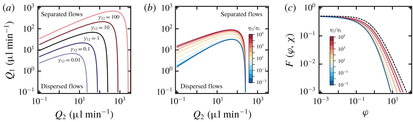
Parameter study of transition curves. (a) Influence of  $\unicode[STIX]{x1D6FE}_{12}$ (
 $\text{mN}~\text{m}^{-1}$) for
 $\unicode[STIX]{x1D70C}_{1}=\unicode[STIX]{x1D70C}_{2}=1~\text{g}~\text{ml}^{-1}$,
 $\unicode[STIX]{x1D702}_{1}=1~\text{cP}$,
 $\unicode[STIX]{x1D702}_{2}=500~\text{cP}$ and
 $h=250~\unicode[STIX]{x03BC}\text{m}$. (b) Role of
 $\unicode[STIX]{x1D712}$. (c) Evolution of
 $F(\unicode[STIX]{x1D711},\unicode[STIX]{x1D712})$ versus
 $\unicode[STIX]{x1D711}$ for various
 $\unicode[STIX]{x1D712}$: solid lines, equation (6.5); dashed line,
 $F(\unicode[STIX]{x1D711},\unicode[STIX]{x1D712})=0.5(1+\unicode[STIX]{x1D711})^{-3/2}$.

We also use this technique to examine the expected influence of interfacial tension  $\unicode[STIX]{x1D6FE}_{12}$ and viscosity ratio
 $\unicode[STIX]{x1D712}$ on flow map transitional lines (figure 12). For a given set of densities and viscosities, the variation of
 $\unicode[STIX]{x1D6FE}_{12}$ modifies
 $M$ as
 $M\sim \unicode[STIX]{x1D6FE}_{12}^{1/2}$, and an increase of the region associated with dispersed flow regimes is observed with increasing
 $\unicode[STIX]{x1D6FE}_{12}$ (figure 12a). In comparison, when all parameters remain fixed while the viscosity ratio
 $\unicode[STIX]{x1D712}$ is manipulated, the transitional lines corresponding to the more viscous inner flow, i.e.
 $\unicode[STIX]{x1D702}_{2}/\unicode[STIX]{x1D702}_{1}\ll 1$ reaches an asymptotic curve for
 $\unicode[STIX]{x1D702}_{2}/\unicode[STIX]{x1D702}_{1}<10^{-1}$ as the size of the highly viscous core becomes invariant to
 $\unicode[STIX]{x1D712}$ in this situation. The calculated transitional curves are also in good agreement with previous experiments of a more viscous core (Cubaud & Mason Reference Cubaud and Mason2008) and closely resemble the transition from dripping droplet flows to jets obtained through linear stability analysis of coaxial flows (Guillot et al. Reference Guillot, Colin, Utada and Ajdari2007; Moiré et al. Reference Moiré, Peysson, Herzhaft, Pannacci, Gallaire, Augello, Dalmazzone and Colin2017). In particular, the analogy between the results previously obtained through linear stability analysis for the dripping–wave transition, which takes place at low outer-stream flow rate, and our criterion based on periodic pattern velocity is remarkable given the two distinct approaches employed and is promising for the development of a unifying framework to advance understanding of multiphase flows in confined microsystems. Over the large range of parameters investigated here, the plunging of the transition curve at large outer-stream flow rate
 $Q_{2}$ is also observed experimentally with the presence of the stable core–annular flows located in the separated flow region (figure 12b). Indeed,
 $Q_{2}^{\ast }\sim Fh^{2}$ remains relatively constant at small
 $\unicode[STIX]{x1D711}$, i.e. at large
 $Q_{2}$ and small
 $Q_{1}$ (figure 12c). While experiments were conducted for various viscosity contrasts
 $\unicode[STIX]{x1D712}$ at relatively fixed interfacial tension
 $\unicode[STIX]{x1D6FE}_{12}$, our analysis suggests the need for additional work on the influence of
 $\unicode[STIX]{x1D6FE}_{12}$ to refine predictive capabilities and further probe the effects of fluid properties and channel geometries on transitional curves.
7 Conclusion
In this work, we present a comprehensive study of various dispersed and separated flow regimes using a single reference microgeometry. Immiscible viscosity-stratified flows with a thin core are produced over a large range of flow rates for various viscosity contrasts using a hydrodynamic focusing section. The use of fluids having low interfacial tension  $\unicode[STIX]{x1D6FE}_{12}$ and different viscosities
 $\unicode[STIX]{x1D712}\ll 1$ enables access to a wide range of flow phenomena to experimentally characterize hydrodynamic instabilities over vast flow maps. Over the range of parameters investigated, dispersed flows are observed for low inner-stream flow rates
 $Q_{1}$ with a dripping–jetting transition based on outer-stream flow rate
 $Q_{2}$, and separated flows are found at large
 $Q_{1}$ with a capillary–inertial wave regime transition depending on
 $Q_{2}$. We systematically investigate the periodic pattern dynamics of droplet trains and interfacial waves with analysis of frequency
 $f$, celerity
 $c$ and wavelength
 $\unicode[STIX]{x1D706}$.
In the dripping regime, we show that droplet length  $d$ and spacing
 $L$ primarily depend on volume fraction
 $\unicode[STIX]{x1D6FC}_{1}$ with minor corrections based on viscosity ratio
 $\unicode[STIX]{x1D712}$ and capillary number
 $Ca_{2}$ of side flow. While the dripping wavelength
 $\unicode[STIX]{x1D706}=d+L$ reaches a minimum at half
 $\unicode[STIX]{x1D6FC}_{1}$, separated flow transition occurs for large
 $d$ and small
 $L$. In the jetting regime, the inner-stream diameter
 $\unicode[STIX]{x1D700}$ of locally stable jets is well predicted analytically, and the frequency of droplet emission
 $f$ is directly proportional to the interfacial velocity or characteristic shear
 $V_{i}/h$ of a stable core. We demonstrate that droplet length
 $d$ depends on flow-rate ratio according to
 $\unicode[STIX]{x1D711}^{1/3}$, and the jetting wavelength
 $\unicode[STIX]{x1D706}$ is in good agreement with the classic theory of capillary breakup at various viscosity ratios
 $\unicode[STIX]{x1D712}$. Another important aspect is the evolution of the aspect ratio
 $d/L$, which quantifies the linear aspect ratio of droplet patterns and collapses all droplet data onto a single curve near the separated flow transition at large flow-rate ratio
 $\unicode[STIX]{x1D711}$.
For waves in the separated flow regime, we analyse the spatial evolution of wavelength  $\unicode[STIX]{x1D706}$ and identify two regimes corresponding to long capillary waves and to small inertial wave patterns. In all cases, data indicate that wave emission frequency is proportional to the interfacial velocity of the primary flow
 $f\sim V_{i}/h$, similar to the jetting regime and previous work on miscible viscous stratifications in microchannels. We then examine the dispersion relationship
 $D(\unicode[STIX]{x1D706},f)$ of capillary waves in qualitative agreement with basic theory and show that the wave aspect ratio
 $\unicode[STIX]{x1D706}/\unicode[STIX]{x1D700}_{2}$, where
 $\unicode[STIX]{x1D700}_{2}$ is the thickness of the viscous layer, provides a useful parameter to account for the role of interfacial curvature and viscosity ratio in the development of capillary waves during separated flows in square microchannels. Then, the wave equation
 $c=\unicode[STIX]{x1D706}f$ is used to derive a functional relationship for the wave celerity as a function of control parameters. We finally discuss wave breaking phenomena, which lead to the formation of ligaments and viscous droplets, and we offer a novel route to continuously emulsify highly viscous materials in small geometries.
The unified description of dispersed and separated flows provides the means to better understand flow transitions. We discuss in particular the evolution of the stable length  $L_{S}$ of base flow configurations with velocity in relation to the development of absolute and convective instabilities. Combining measurements of frequency
 $f$ and wavelength
 $\unicode[STIX]{x1D706}$ across all regimes highlights the role of the capillary number and the flow-rate ratio in pattern selection. In turn, this work shows that droplet velocity
 $V_{D}$ and wave celerity
 $c$ meet at their highest value at the flow transition. A criterion based on periodic pattern velocity is then developed to predict the critical flow rates for transition in good accord with experimental data, which provides a complementary approach to linear stability analysis.
Overall, this study clarifies the role of fluid properties in the development of a wide range of microfluidic instabilities. Amongst various regimes of interest, the jetting regime displays dual properties between the dripping and wave regimes, and the periodic flow velocity is shown to play a major role in pattern selection. Further theoretical and computational work would help to better understand hydrodynamic flow transitions to improve the design of microfluidic flow devices in a variety of situations. Here, the wave regime and wave breaking behaviour expand the scope of previously known microflow regimes and provide new opportunities for microfluidic applications.
Acknowledgement
This material is based upon work supported by the National Science Foundation under grant no. CBET-1150389.
Declaration of interests
The authors report no conflict of interest.