I. INTRODUCTION
The flow or creep of polycrystalline materials at elevated temperatures is now understood reasonably well. When a material is subjected to a constant stress or load that is below the fracture stress, the material gradually deforms with time until it ultimately fails. Generally, there is an initial instantaneous strain on application of the load and this is followed by a primary stage of creep where the creep rate decreases with increasing time, a steady-state region where the creep rate remains essentially constant and then a tertiary stage where the creep rate accelerates up to the point of failure. Often much of the flow occurs under steady-state conditions and then an important requirement, for any selected testing conditions, is to determine the rate-controlling flow mechanism. Extensive reviews are now available describing the nature of the flow processes occurring under creep conditions.Reference Kassner and Pérez-Prado1, Reference Kassner2
Creep is a diffusion-controlled process occurring at temperatures above ∼0.5 T m, where T m is the absolute melting temperature. Extensive experiments have established that the steady-state creep rate,  ${{\dot \varepsilon }}$, may be expressed by a simple relationship of the formReference Bird, Mukherjee, Dorn, Brandon and Rosen3, Reference Langdon4
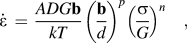 $${{\dot \varepsilon }}\, = \,{{ADG{\bf{b}}} \over {kT}}\left( {{\bf{b} \over d}} \right)^p \left( {{{\rm{\sigma }} \over G}} \right)^n \quad,$$
where D is the appropriate diffusion constant [= D 0exp(−Q/RT), where D 0 is the frequency factor, Q is the activation energy for the flow process, R is the gas constant, and T is the absolute temperature], G is the shear modulus, b is the Burgers vector, k is Boltzmann's constant, d is the grain size, σ is the flow stress, n and p are the exponents of the stress and the inverse grain size, respectively, and A is a dimensionless constant.
It follows from inspection of Eq. (1) that the creep behavior is governed by three separate experimental parameters: the testing temperature, T, the applied stress, σ, and the grain size of the material, d. Therefore, the magnitudes of these parameters play a critical role in dictating the rate of flow. In creep experiments, it is a standard procedure to measure the dependence of the creep rate on these parameters and then to estimate the rate-controlling mechanism. However, an alternative and preferred approach is to attempt to construct a pictorial display that depicts the rate-controlling mechanisms over a range of experimental conditions. This type of diagram is known as a “deformation mechanism map” and it follows from a concept first introduced in materials science almost 50 years ago. The principles of deformation mechanism maps are described in the following section and the subsequent sections describe alternative mapping procedures including an alternative approach to fracture mechanisms, the additional complexities associated with the mapping of ceramic materials and the potential for extending this same approach to ultrafine-grained and nanostructured materials where the grain sizes are in the submicrometer or nanometer ranges.
II. BASIC PRINCIPLES OF DEFORMATION MECHANISM MAPPING
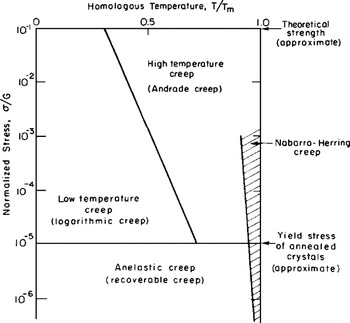
The possibility of displaying flow mechanisms pictorially was first suggested in the 1960s and the result is shown in Fig. 1.Reference Weertman, Weertman and Cahn5, Reference Weertman6 In this creep diagram, the normalized stress, σ/G, is shown as a function of the homologous temperature, T/T m, from absolute zero to the melting temperature. The upper line at σ/G = 10−1 was taken as the approximate theoretical strength of the material and the lower horizontal line at σ/G = 10−5 was placed equal to the approximate yield stress of annealed crystals. Between these two extremes, the behavior was divided into high temperature (HT) or Andrade creep and low temperature (LT) or logarithmic creep, with the additional occurrence of Nabarro–Herring diffusional creepReference Nabarro7, Reference Herring8 at very HTs. At normalized stresses below 10−5, the behavior was anelastic or recoverable.
The creep diagram as first proposed in the 1960s.Reference Weertman, Weertman and Cahn5, Reference Weertman6

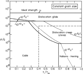
The creep diagram in Fig. 1 provides a useful overview of the general trends associated with creep mechanisms but the approach was significantly refined in 1972 through the construction of deformation mechanism maps which provided an overall representation of the flow processes with a high degree of accuracy.Reference Ashby9 A schematic example of this approach is shown in Fig. 2 where the normalized stress, σ/G, is plotted against the homologous temperature, T/T m, for a constant grain size.Reference Langdon and Mohamed10 In this illustration, the normalized stress covers eight orders of magnitude from 10−8 to 1.0 and the upper line at σ/G ≈ 4 × 10⁻² denotes the ideal strength of the material. The lower bold lines denote field boundaries and they represent the loci of all points where the two adjacent processes have equal strain rates. The fields correspond to regions in stress–temperature space wherein a single flow mechanism is rate controlling. The upper field marked dislocation glide extends from the ideal strength to ∼4 × 10⁻³ and denotes the stress–temperature regime where the material deforms by the conservative motion of dislocation glide. At σ/G < 4 × 10⁻³, the flow behavior is due to diffusion-controlled creep mechanisms ranging from dislocation creep due to climb to Nabarro–HerringReference Nabarro7, Reference Herring8 and CobleReference Coble11 diffusion creep. The two thin lines superimposed in Fig. 2 correspond to representative contours of strain rate for 10−2 and 10−10 s−1.
Schematic illustration of the conventional deformation mechanism map of normalized stress versus homologous temperature.Reference Langdon and Mohamed10

Figure 2 shows a schematic illustration of the basic principles of deformation mechanism mapping but in practice, separate maps may be constructed for any selected material. This approach was developed extensively so that, in 1982, a compendium of maps was published covering a wide range of f.c.c., b.c.c., and h.c.p. metals, various nonferrous and ferrous alloys, and a number of nonmetallic systems including oxides, geological materials, and ice.Reference Frost and Ashby12
III. A SIMPLIFIED APPROACH TO MAPPING
Although maps of the type shown in Fig. 2 are now well established, they have a significant limitation because of the difficulties associated with their construction. Typically, a map is constructed by considering the constitutive equation for every possible flow mechanism and then solving these relationships at several thousand points in stress–temperature space. An additional limitation is that maps of the type shown in Fig. 2 apply only to a specific grain size and there is no quick and easy procedure for constructing another map for the same material having a different grain size. Because of these inherent difficulties, alternative approaches were developed with the specific objective of illustrating the dominant mechanisms occurring in HT creep that corresponds essentially to homologous temperatures covering the range from 0.4 to 1.0 T m and normalized stresses <10−3: this region is delineated by the broken lines in Fig. 2.
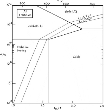
A simple procedure for modifying basic maps of the type shown in Fig. 2 is to plot the flow processes in the form of the normalized stress, σ/G, against the reciprocal of the homologous temperature, T m/T, at a constant grain size.Reference Langdon and Mohamed10 In this form, all field boundaries and strain rate contours appear as straight lines. An example is shown in Fig. 3 for pure Al having a grain size of 100 μm and using the constitutive relationships for HT climb controlled by lattice diffusion, LT climb controlled by core diffusion, and Nabarro–HerringReference Nabarro7, Reference Herring8 and CobleReference Coble11 diffusion creep.Reference Langdon13 The two strain rate contours for 10−9 and 10−10 s−1 denote an essentially lower limiting rate of ∼0.01%/day for laboratory experiments and an upper limit of ∼3%/10 years for most structural design purposes. In practice, however, it is a simple procedure to add additional strain rate contours because all contours are parallel and equally spaced within each field.
A simplified map of normalized stress versus the inverse of homologous temperature for Al having a grain size of 100 μm.Reference Langdon13

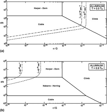
Figure 3 again relates to only a single grain size but an alternative approach, following Eq. (1), is to plot the normalized grain size, d/b, against the normalized stress, σ/G, at constant temperature.Reference Mohamed and Langdon14 Examples are shown in Fig. 4 for aluminum at homologous temperatures of (i) 0.5 T m and (ii) 0.9 T m and using the constitutive relationships for dislocation climb, Nabarro–HerringReference Nabarro7, Reference Herring8 and CobleReference Coble11 diffusion creep, and Harper–DornReference Harper and Dorn15 creep: again the maps include two representative strain rates of 10−9 and 10−10 s−1 but with a curvature included to denote the additive nature of the two mechanisms on either side of each field boundary.Reference Mohamed and Langdon16 Similar maps have also been developed for solid solution alloysReference Mohamed and Langdon17 and superplastic materials.Reference Mohamed and Langdon18
Simplified maps of normalized grain size versus normalized stress for Al at (a) 0.5 T m and (b) 0.9 T m.Reference Mohamed and Langdon16

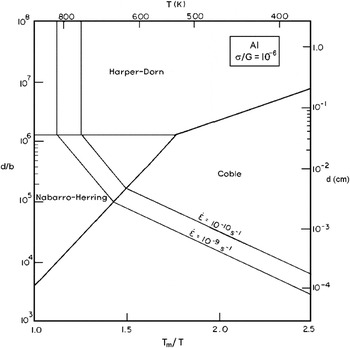
Since there are three separate experimental parameters in Eq. (1), it is apparent that there is also a third type of map in which the normalized grain size is plotted against the inverse of the homologous temperature, T m/T, at constant normalized stress.Reference Langdon and Mohamed19 An example is shown in Fig. 5 for aluminum at σ/G = 10−6 where the values of the grain sizes are shown on the right-hand axis.Reference Langdon13
Simplified map of normalized grain size versus the inverse of homologous temperature for Al at a normalized stress of 10−6.Reference Langdon13

In summarizing these basic forms of deformation mechanism maps, it is important to note that the maps are only as accurate as the data used in their construction. This means that any inaccuracies in the fundamental constitutive relationships, or in the experimental values used for the various terms within these relationships, will necessarily introduce errors in the maps. Thus, although the maps are a very valuable aid in displaying possible creep mechanisms, some care must be exercised in using the maps to make predictions on flow behavior.
IV. FURTHER EXTENSIONS OF THE MAPPING APPROACH
A. Mechanisms of fracture
The preceding sections relate to the display of deformation mechanisms in the form of maps but a similar approach is possible also for fracture mechanisms. The possibility of displaying failure modes in the form of a fracture diagram in strain rate–temperature space was first suggested many years agoReference Wray20 and subsequently the concept was developed into the form of fracture maps in which the dominant fracture mechanisms are displayed in a plot of normalized stress against homologous temperature.Reference Ashby and Raj21
As shown earlier in Fig. 3, this type of mapping may be simplified by plotting the data in the form of the normalized stress, σ/G, against the reciprocal of the homologous temperature, T m/T for a constant grain size. An example is given in Fig. 6 for 316 stainless steel having a grain size of 150 μm.Reference Miller and Langdon22 The fracture mechanisms depicted in Fig. 6 are transgranular creep failure with both LT and HT variations, triple point cracking, and cavitation failure either through the diffusion growth of cavities or through power-law growth due to deformation in the surrounding matrix. Also included in Fig. 6 are four contours showing constant times to failure, t f, from 106 to 109 s.
A fracture map of normalized stress versus the inverse of homologous temperature for 316 stainless steel having a grain size of 150 μm.Reference Miller and Langdon22

B. The development of mapping for ionic solids
The same approach may be used also for the mapping of ceramic materials.Reference Langdon and Mohamed23–Reference Langdon25 However, the situation is then more complicated because of the presence of ambipolar diffusion in Nabarro–Herring and Coble diffusion creep in which there is a simultaneous mass transport of anions and cations along parallel, but different, diffusion paths.Reference Gordon26, Reference Gordon and Hodge27 In ambipolar diffusion, the total flow associated with each ionic component remains in the stoichiometric ratio but the net current flow along each parallel diffusion path is not necessarily zero. This leads to a more complex diffusion coefficient because it is necessary to consider both lattice and grain boundary diffusion, identify the faster diffusion path for both the anions and the cations, and then determine the slower of these two processes to obtain the rate-controlling mechanism.
Using this approach, it is possible to construct deformation mechanism maps for diffusional creep in ceramic materials. An example is shown in Fig. 7 for Al2O3 using the form of mapping depicted earlier in Fig. 5 where the normalized grain size is plotted against the inverse of the homologous temperature.Reference Langdon and Mohamed24 The map is now divided into four separate fields denoting the possible flow processes in the diffusional creep of ionic solids. Specifically, cation-controlled Coble creep is dominant at small grain sizes and lower temperatures, there is a transition to cation-controlled Nabarro–Herring creep with increasing temperature and grain size, then anion-controlled Coble creep, and finally, at very large grain sizes and temperatures close to the melting point, to anion-controlled Nabarro–Herring creep. Since Nabarro–Herring and Coble creep both have the same dependence on stress, the field boundaries in this map are independent of the stress level. However, it is possible to select a stress and then insert the appropriate strain rate contours. An example is shown in Fig. 5 where the normalized stress is taken as σ/G = 10−3 and two representative strain rate contours are inserted for 10−9 and 10−10 s−1.
A deformation mechanism map for diffusion creep in Al2O3 showing the four diffusional creep processes and two strain rate contours for a normalized stress of 10−3.Reference Langdon and Mohamed24

V. USING DEFORMATION MECHANISM MAPS FOR ULTRAFINE-GRAINED AND NANOSTRUCTURED MATERIALS
A. Principles of mapping for ultrafine-grained materials
The deformation mechanism maps available in the literature generally relate to relatively large grain sizes. For example, the grain size of d = 100 μm in Fig. 3 is typical of the maps now available. Nevertheless, the development of new processing techniques and the availability of materials with submicrometer and nanometer grain sizes has promoted an interest in developing maps for ultrafine-grained materials.
Processing by equal-channel angular pressing (ECAP)Reference Valiev and Langdon28 and high-pressure torsion (HPT)Reference Zhilyaev and Langdon29 are two techniques in which the grains of bulk solids may be refined to give grain sizes typically in the submicrometer range of 0.1–1.0 μm. Since the processed materials are reasonably large, it is a simple procedure to cut and test the as-processed samples in tension at elevated temperatures. Many of the results for these ultrafine-grained materials show the occurrence of superplastic elongations with ductilities up to >1000%Reference Kawasaki and Langdon30 and therefore, it is important to develop deformation mechanism maps to depict these flow properties. A theoretical model is available for superplastic flow in conventional large-grained materialsReference Langdon31 and a recent study showed this model is in excellent agreement also with the superplastic flow reported in ultrafine-grained materials.Reference Kawasaki, Balasubramanian and Langdon32 Accordingly, using the conventional creep mechanisms, a series of maps was constructed and it was shown that they are in excellent agreement with materials processed by ECAPReference Kawasaki, Lee and Langdon33–Reference Kawasaki and Langdon36 and HPT.Reference Kawasaki and Langdon37, Reference Kawasaki and Langdon38
Examples of this approach are given in Fig. 8 where the normalized grain size is plotted against the normalized stress for the Zn-22% Al eutectoid alloy tested in tension at a temperature of 473 K and the results are shown by taking experimental data for this alloy after processing by (i) ECAPReference Kawasaki and Langdon39 and (ii) HPT.Reference Kawasaki and Langdon37 The regions designated as I, II, and III in Fig. 8 represent the three regions of flow generally associated with superplastic materials including the Zn-22% Al eutectoid alloy,Reference Ishikawa, Mohamed and Langdon40, Reference Mohamed and Langdon41 the fields labeled Nabarro–Herring and Coble are based on the theoretical models for these processes,Reference Nabarro7, Reference Herring8, Reference Coble11 and the broken line where the normalized grain size is equal to 20(σ/G)−1 represents the condition where the sample grain size is equal to the subgrain size based on an analysis of extensive creep data for a large number of metals.Reference Bird, Mukherjee, Dorn, Brandon and Rosen3 The maps were constructed using b = 2.7 × 10⁻¹⁰ m,Reference Langdon and Mohamed42 and G = {4.797 × 10⁴—(2.662 × 10T)} MPa.Reference Mohamed, Shei and Langdon43 The experimental points shown in Fig. 8(a) are taken from data reported earlier for the Zn-22% Al alloy processed by ECAP to give a grain size of 1.74 μmReference Kawasaki and Langdon39 and these points lie correctly within the superplastic region II and in regions I and III where there are transitions to nonsuperplastic behavior. Similarly, the experimental points shown in Fig. 8(b) are for the same alloy processed by HPT to give a grain size of 610 nm and again these points lie within the correct regions. Thus, these plots confirm the potential for constructing realistic deformation mechanism maps for materials having ultrafine submicrometer grain sizes. These grain sizes are easily produced by ECAP and HPT and by other processes such as friction stir processing.Reference Liu and Ma44
Deformation mechanism maps of normalized grain size versus normalized stress for the Zn-22% Al eutectoid alloy at 473 K showing experimental data for (a) testing by ECAPReference Kawasaki and Langdon39 and (b) testing by HPT.Reference Kawasaki and Langdon37

B. Principles of extending the maps for materials with nanometer grain sizes
A further extension of this approach to materials having grain sizes within the true nanometer range requires a detailed understanding of the deformation mechanisms occurring at these very small grain sizes. There is good evidence for changes in the conventional flow processes when the grain size is within the nanometer rangeReference Mohamed and Chauhan45–Reference Mohamed and Yang48 and, as described in a recent report,Reference Mohamed49 this will entail adding other mechanisms to the maps such as nanograin deformationReference Mohamed and Yang48 and triple junction diffusion creep.Reference Wang, Wang, Aust and Erb50 Also, there is evidence for new mechanisms in these materials from both molecular-dynamics simulationsReference Van Swygenhoven51–Reference Van Swygenhoven, Derlet and Frøseth53 and experiments.Reference Chen, Ma, Hemker, Sheng, Wang and Cheng54–Reference Zhu, Wu, Liao, Narayan, Mathaudhu and Kecskés57 For example, partial dislocations may be emitted from the grain boundaries in these nanostructured materials and this leads to the formation of deformation twins. Very recent results suggest evidence for a critical stress controlling the production of nano-twinned microstructures.Reference Cao, Wang, Liao, Kawasaki, Ringer, Langdon and Zhu58
An additional characteristic of these nanostructured materials is the presence of nonequilibrium grain boundaries having an excess of extrinsic dislocations.Reference Valiev59 The presence of these dislocations has been well-established using high-resolution electron microscopyReference Horita, Smith, Furukawa, Nemoto, Valiev and Langdon60, Reference Horita, Smith, Nemoto, Valiev and Langdon61 but their precise role in the deformation behavior is not yet understood. Finally, there is evidence also that grain boundary sliding may become an important flow process when the grain size is significantly reduced.Reference Chinh, Szommer, Horita and Langdon62–Reference Chinh, Csanádi, Györi, Valiev, Straumal, Kawasaki and Langdon64 It is apparent from this summary that more experimental results are needed to precisely delineate the flow processes in the nanometer range. Nevertheless, it would be instructive, in the first instance, to construct deformation maps for these small grain sizes based on conventional deformation mechanisms and to use these maps to identify any major deviations that are occurring due to the use of nanometer grain sizes.
VI. SUMMARY AND CONCLUSIONS
1. The construction of deformation maps is a simple procedure for providing a visual display of the anticipated deformation mechanisms occurring under any selected conditions. A range of simplified maps is available based on the three experimental parameters of stress, temperature, and grain size. Similar maps may be constructed also for creep fracture mechanisms or to show the presence of ambipolar diffusion in ionic solids.
2. Only a limited number of maps has been constructed for materials having ultrafine submicrometer grain sizes but nevertheless the maps available to date are in excellent agreement with the experimental data.
3. No attempt has been made to date to construct maps for materials having true nanometer grain sizes but the evidence suggests that it is then necessary to include additional flow mechanisms such as nanograin deformation and triple junction diffusion creep.
ACKNOWLEDGMENTS
This work was supported in part by the National Science Foundation of the United States under Grant No. DMR-1160966 and in part by the European Research Council under ERC Grant Agreement No. 267464-SPDMETALS.