1. Introduction

Batterman's remarkably insightful recent book, The Devil in the Details: Asymptotic Reasoning in Explanation, Reduction, and Emergence, develops a number of salutary themes—among them, the importance of stability results in the explanation of physical phenomena and the fruitfulness of simultaneous engagement with issues in general philosophy of science and with details of a variety of physical theories (Batterman Reference Batterman2002).Footnote ¹

But the most provocative theme of the book is that fundamental physical theories can be expected to be explanatorily inadequate—that there exist phenomena that can be understood only when the conceptual apparatus of a fundamental theory is supplemented by concepts whose natural home is in a less fundamental theory. Batterman's route to this claim begins with a discussion of the classical philosophical accounts of explanation and reduction, leads through considerations surrounding the asymptotic analysis of the differential equations of optics and quantum mechanics, and ends with an argument that attention to such considerations should transform our view of the role of less-than-fundamental theories in our knowledge of the world.

This paper follows a similar trajectory. By way of providing a backdrop for Batterman's project, I begin in Section 2 with a discussion of explanation and reduction. I then consider, in Sections 3 and 4, the examples from optics and mechanics upon which Batterman bases his case. Finally in Section 5, I turn to Batterman's argument for his thesis that fundamental theories are typically explanatorily inadequate, and suggest a line of objection to this argument.

Perhaps it will be helpful if I provide a preliminary indication here of this line of objection. Batterman holds it to be a shortcoming of the older methodological literature on explanation and reduction that it proceeds at a high level of abstraction. Batterman is one of a number of contemporary writers on these topics who insists that adequate methodological accounts must be built upon a careful examination of the complexities of genuine examples of scientific research. This is one of the senses in which the devil is in the details for Batterman: only by working through detailed examples will we learn certain important lessons that we cannot afford to ignore.Footnote ² In Sections 3 and 4 I am going to discuss in some detail the examples that Batterman bases his case upon—but I will in Section 5 draw a lesson different from his. To put the matter roughly and tendentiously: I am going to focus for the most part on the sort of details that figure in mathematicians’ treatments of these examples, where Batterman tends to draw his details from physicists’ accounts; I am going to charge Batterman with following physicists in thinking of less fundamental theories as making an ineliminable contribution to our understanding of certain phenomena when consideration of the mathematicians’ approach would show that such theories make only a heuristic and eliminable contribution.Footnote ³ Of course, I will also have to fend off the counter-accusation that I mistake bloodless formalities for genuine physical understanding.

2. Background

Let us say that one physical theory supersedes another if almost all of the phenomena treated adequately by the latter are afforded a superior treatment by the former (here the term ‘phenomena’ may cover, in addition to observable facts and regularities, unobservable ones whose status is taken to be unproblematic in the context at hand).

We can divide historical examples of superseded theories into two categories: dead letters and theories emeritus. Theories in the former class remain the subject of serious intellectual interest only among historians and antiquarians, while those falling in the latter continue to play a role in the education and research of mathematicians and physicists.Footnote ⁴ A plausible conjecture is that this distinction can be grounded as follows: Any superseded theory will be able to count among its lasting achievements some degree of empirical adequacy; for dead letters, the list will end there; but theories emeritus will also have lasting explanatory achievements to their credit. Thus, while the value of a Ptolemaic account of a celestial phenomenon (eclipses, say) is exhausted by the naked-eye accuracy of the predictions of the theory, the value of a geometrical optical account of some phenomenon (burning mirrors, say) may lie in the explanatory power of that account, as well as in its empirical adequacy.

We can view the classical approach to reduction as an attempt to provide an account of the logical relation between theories emeritus and their supersessors, in light of which the explanatory power—and pragmatic status—of each theory emeritus is fully vindicated.Footnote ⁵ According to this approach, we expect that, for good $T_{1}$ and $T_{0}$ , if $T_{1}$ supersedes $T_{0}$ , then it is possible to construct within $T_{1}$ a deductive-nomological explanation of the laws of $T_{0}$ —that is, a derivation of the laws of $T_{0}$ from the laws of $T_{1}$ , supplemented where necessary by assertions of particular fact. Now, in interesting cases, this will be impossible: the laws of $T_{0}$ involve terms alien to $T_{1}$ in a manner which renders the desired deduction impossible. To meet this difficulty, we allow ourselves to extend $T_{1}$ by adding new laws, informally understood as correlating the alien terms of $T_{0}$ with expressions native to $T_{1}$ .Footnote ⁶ We then say that $T_{0}$ reduces to $T_{1}$ if it is possible to explain, in the desired fashion, the laws of $T_{0}$ within the extended theory.Footnote ⁷

Reductionism is sometimes associated with eliminativism—the idea being that to show that the laws of a given theory are just consequences of the laws of one of its supersessors is to show that the theory is in principle dispensable and its ontology derivative. But Nagel and Hempel themselves appear to deny that a successful reduction of, say, biology to chemistry, or of psychology to neurophysics, or of the framework of every day experience to fundamental physics, would show that reality accrued only to the objects of the more fundamental member of the pair.Footnote ⁸ On their view, a successful reduction shows not that the reduced theory need be discarded, but that it is safe to go on using it. For, one has on the authority of the superseding theory the trustworthiness of the predictions of the superseded theory.Footnote ⁹ And it will be safe to go on employing the superseded theory in generating deductive-nomological explanations—since the laws of the superseded theory are just theorems of (a pertinent extension of) the superseding theory; explanations arising in this way will count as explanations from the perspective of the superseding theory.Footnote ¹⁰ When this obtains, one has license to continue employing the concepts and laws of the superseded theory. Thus reductions of our theories emeritus to fundamental physical theories would explain why theories emeritus are kept on the books.

But here a well-known problem arises—there are, in fact very few examples of reduction in the strict classical sense.

Consider the relation between Galileo's law of free fall and Newton's theory of gravitation. Nagel offers this as an example of a successful reduction.Footnote ¹¹ In Newtonian mechanics, Galileo's law of free-fall holds only for bodies subject to a uniform gravitational force. But Galileo's treatment is meant to hold of bodies near the earth, where the strength of the gravitational field increases as the surface of the earth is approached. Now, Nagel's account of explanation of laws (Reference Nagel1961, 42–43), like Hempel's canonical deductive-nomological account, requires the truth of the explanans. And so, strictly speaking, there is no explanation of Galileo's law of free-fall in Newtonian mechanics. Rather, one can either: (i) derive the superseded law by supplementing the laws of the superseding theory by false empirical assumptions; or (ii) derive from true empirical assumptions together with the laws of the superseding theory a statement that, in a suitable sense, approximates the superseded law, for a range of conditions.

Similar objections apply to the other candidates for reductions proposed by Nagel—the relation between the kinetic theory of gases on the one hand and the Boyle-Charles law and the second law of thermodynamics on the other.Footnote ¹² Indeed, the problem is very general: A theory reduces to one of its supersessors only if it is in fact a special case of that supersessor. Perhaps the wave theory of light can be understood as being a special case of Maxwell's theory in the relevant sense. But this phenomenon is very rare—it is far more common for a theory to be corrected by its supersessors, even within its range of empirical adequacy. This will be the case, for instance, whenever we say that one theory is the limit of the other—as in the relation between geometrical optics and wave optics, classical mechanics and relativistic mechanics, classical mechanics and quantum mechanics, or special relativity and general relativity. In each of these cases, reduction fails because the supersessor, rather than implying the laws of the superseded theory, offers corrections to them.Footnote ¹³

It is at this point that the eliminativism of Feyerabend (Reference Feyerabend, Feigl and Maxwell1962, Reference Feyerabend, Cohen and Wartofsky1965) and Sellars (Reference Sellars, Feigl and Maxwell1961, Reference Sellars, Cohen and Wartofsky1965) gets its foot in the door. The fact that our less fundamental theories (including the ‘theory’ of common sense) do not reduce to our more fundamental theories shows that the former are, strictly speaking, false. At present, we keep them on the books for pragmatic reasons—they simplify calculations. But it will ultimately be desirable to strike them from the books, and educate ourselves to think in the framework of fundamental physics—only thus will we be able to see our way past the pseudo-problems and philosophical dead ends that are suggested by these false conceptualizations of the world.

It is only natural to wonder whether this isn't an over-reaction to the failure of Nagelian reduction. Mightn't there be a somewhat weaker relation that holds between our theories emeritus and their more fundamental successors, which offers us something more than pragmatic reason to keep the former on the books? Couldn't there still be something to the idea that theories emeritus differ from dead letters in offering genuine explanatory insight?

Under pressure from objections to their account of reduction, Hempel and Nagel suggested that we might want to introduce a notion of approximative reduction: roughly, we would say that a regularity could be approximatively explained by a given theory when the laws of that theory allow us to deduce a near-relative of the regularity; and that one theory approximatively reduces to another if the latter supports appropriate approximative explanations of the laws of the former.Footnote ¹⁴ This provides the outline of a program for grounding the status of theories emeritus. But this program remains largely unfulfilled. Indeed, there are daunting obstacles to be faced—in addition to the problems that bedevil the notion of explanation, one has to worry about what counts as an acceptable approximation to a regularity of a theory to be approximatively reduced. And this is likely to lead one away from the abstractions that were the stock in trade of the logical empiricists, and towards the messy mathematical details of the limiting relations between particular theories—undermining any hope for a clean and general account of the status of theories emeritus.

Batterman promises to cut through this Gordian knot of difficulties. He examines the relation between geometrical optics and wave optics and the relation between classical mechanics and quantum mechanics, and concludes that in each case the more fundamental superseding theory is explanatorily inadequate—that there are phenomena whose understanding requires that the conceptual resources of the more fundamental theory be supplemented by those of the less fundamental theory.Footnote ¹⁵ The considerations that drive Batterman's analysis turn crucially upon the complexity of the limiting relation between the pairs of theories that he considers (and it is plausible that the argument, if successful, can be carried over to other theories emeritus). Thus methodologists should find cause for joy rather than grief in the failure of classical reduction in these cases. For, this failure opens up a royal road towards the establishment of the explanatory credentials of certain superseded theories, bypassing entirely the muskeg of approximate laws and approximate truth and the strengths and weaknesses of the variety of explanation that they support.

Batterman offers a reason for keeping geometrical optics and classical mechanics on the books that goes far beyond a mere pragmatic interest in calculational tractability—namely, that these theories play an ineliminable role in our understanding of the physical world. How does this work? In the next two sections, I discuss the two examples that Batterman focuses upon.

3. Example: The Rainbow

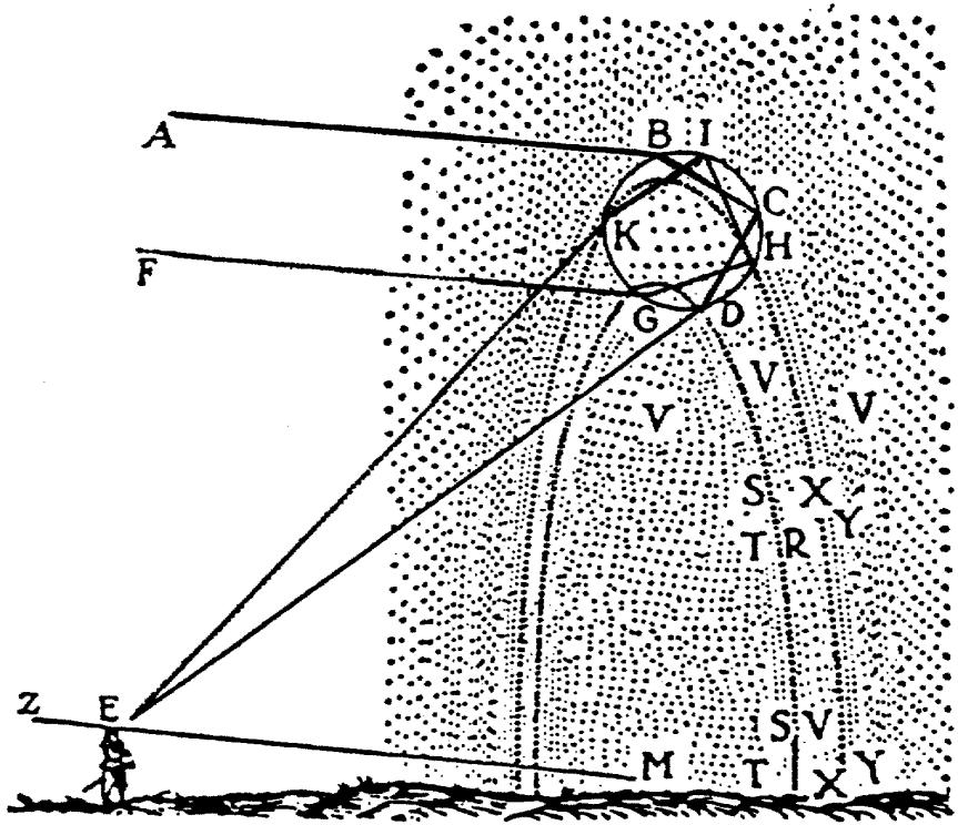
Let's begin with (the successful bits of) Descartes’ account of the rainbow in the Eighth Discourse of his Meteors. Suppose that you find yourself in the situation depicted in Descartes’ diagram (see Figure 1): You stand wearing a velvet suit and a sword, looking towards a spherical droplet of water suspended in the air, which is illuminated by light source behind you. We will assume that the light is of a single wavelength. We are interested in the light that enters the raindrop from the left, undergoes a sequence of refractions and internal reflections, and exits the raindrop traveling towards the left. Let us call such a ray primary if it exits the drop after a single internal reflection, secondary if it exits after two internal reflections, and so on.

Figure 1.

Descartes' diagram, from the Eighth Discourse of his Meteors. Here, ray ABCDE is primary, and ray FGHIKE is secondary.

Descartes’ strategy is to imagine 10,000 evenly spaced rays parallel to AB, each considered as an initial segment of a primary ray, and, for a plausible value of the refractive index of water, to calculate the angle between the initial and final segments of the ray. That is, he wants to calculate angles like the angle DEM of his diagram—that angle is, of course, the same as the angle between AB and DE. His conclusion: “I found that after one reflection and two refractions, very many more of them can be seen under the angle of 41° to 42° than under any lesser one; and that none of them can be seen under a larger angle” (Olscamp Reference Olscamp1965, 339). Similarly, Descartes considers the secondary rays and finds that “very many more of them come toward the eye under a 51° to 52° angle, than under any larger one; and no such rays come under a lesser” (339).

If we suppose now that the observer faces a cloud of spherical water droplets, illuminated from behind by our light source, we can study the patterns of illumination which result from primary and secondary rays from each of the droplets. Describing the position of raindrops in the cloud by the angle that a line joining them makes to the continuation past the observer of a line from the sun to her eye, it follows from Descartes’ analysis that many primary rays will reach the eyes from drops along the circular band corresponding to 41° to 42°. This band is theprimary bow. Its inner side is lit by primary rays—but with the intensity falling off rapidly as the angle decreases. Similarly, the secondary bow consists of an illuminated band at 51° to 52°, with a lit outer side (with the intensity falling off rapidly as the angle increases). The region from 42° to 51° is unlit by primary and secondary rays.

Aside from failing to treat chromatic phenomena, this approach gives a good rough account of some of the most conspicuous features of naturally occurring rainbows.Footnote ¹⁶

The 19th century wave-theoretic analysis of the rainbow, due to Airy and others, predicts the following departures from the geometrical treatment.Footnote ¹⁷

• • The dark band is faintly illuminated near the outside (inside) of the primary (secondary) bow, although this tails off quickly away from the bow.

• • The peak in intensity of the primary (secondary) bow occurs at an angle less than (greater than) the angle predicted by the geometrical-optical account.

• • Within the illuminated region one finds, rather than the monotonic decrease in intensity predicted by the geometrical-optical account, a series of minor peaks in intensity—these are known as the supernumerary bows.

• • In the geometrical-optical account, the positions of the primary and secondary bows are fixed by the refractive index of water (together with the assumption that the drops are perfectly spherical). In the wave-theoretic account, the position of the bows depends on the size of the water droplets.Footnote ¹⁸

Each of these is borne out by observation—indeed, except for the first, each can be verified at the level of naked-eye observation.

So far, then, we have a familiar sort of story: A good theory giving a good account of a phenomenon of interest is superseded by an even better theory giving an even better account of that phenomenon. Batterman claims that, contrary to appearances, the wave-theoretic account of the rainbow is explanatorily inadequate, and that understanding of this phenomena requires the mobilization of resources from geometrical optics.

Why? Well, let's start by asking what we expect from a scientific explanation of a phenomenon such as the rainbow. Hempel (Reference Hempel1966, 48) advocates the plausible view that what is characteristic of scientific explanation is that “the explanatory information adduced affords good grounds for believing that the phenomenon to be explained did, or does, indeed occur. This condition must be met if we are to be entitled to say: ‘That explains it—the phenomenon in question was indeed to be expected under the circumstances!’” By way of example:

Waiving questions of the truth of the laws of geometrical optics, does Descartes’ account of the rainbow amount to an explanation in the desired sense? Well, Descartes shows something like: Under normal conditions, a rainbow appears when a cloud of spherical droplets is lit by a bright light behind the observer. So, it remains to show either that the drops in a mist or spray can be expected to be spherical, or that nonspherical drops lead to similar optical phenomena.Footnote ¹⁹ In fact, falling raindrops of the size of several millimeters have shapes that depart appreciably from the spherical (Pruppacher and Klett Reference Pruppacher and Klett1997, Section 10.3.2). So we are stuck trying to show something like: Any spray or mist that we come across is likely to produce a pattern of illumination very similar to that produced by a cloud of spherical drops.Footnote ²⁰

One way that this could be achieved would be via a structural stability result, according to which perturbations of the shape of the drops lead to relatively tame differences in the structure of appearances. Batterman (89–93) considers one such strategy, under which one shows that in the limit of high frequency, generic perturbations of the shape of the drop away from sphericity lead to a pattern of intensities closely related to that for a spherical drop. This story comes in several parts.

First Part: The Basic Integrals. Footnote ²¹ As a harmless simplification we study the wave equation, $[ (\partial ^{2}/\partial t^{2}) -\triangle ] u=0$ , instead of Maxwell's equations (allowing us to focus on a scalar, rather than a vector, quantity). If we consider a point source located at $y\in \mathstrut{\Bbb R} ^{3}$ , emitting light of frequency k and amplitude $a\in \mathstrut{\Bbb C} $ , then

describes the radiation reaching a point $x\in \mathstrut{\Bbb R} ^{3}$ ( $x\neq y$ ) at time t. Now suppose that we have a compact (i.e., closed and bounded) surface, S, in $\mathstrut{\Bbb R} ^{3}$ and that each point y on S emits light of frequency k and amplitude $a(y) $ and that these emitters are in phase with one another. Then the radiation at $x\in \mathstrut{\Bbb R} ^{3}$ ( $x\not\in S$ ) at time t is given by

So we have, for certain sets of emitters on S, an integral expression for a solution to the wave equation everywhere off of S. Since the only dependence on t is via the boring factor out front, we will from now on focus on the integral, calling it $I_{k}(x) $ ; $\vert I_{k}(x) \vert ^{2}$ gives the intensity of light at x.

We are interested in certain qualitative aspects of the behavior of light that can be understood by studying the behavior of $I_{k}(x) $ in the high-frequency limit as $k\rightarrow \infty $ . Notice that as k grows large, the integrand begins to oscillate wildly. But the behavior of the integral itself can be surprisingly simple—this is the purport of some 19th century results, normally grouped together under the moniker the principle of stationary phase.

I state some of these results for a class of integrals that includes our special $I_{k}(x) .$

We consider integrals of the form $\mathstrut{\cal I} _{k}(x) =\int_{S}e^{ik\varphi (x,y) }a(x,\,y,\,k) dy$ , defined for $k> 0$ , x in some open subset of $\mathstrut{\Bbb R} ^{3}$ , y in some open subset of $\mathstrut{\Bbb R} ^{2}$ ; with ϕ real and a complex and vanishing for y outside of some compact set, S.Footnote ²² We call a the amplitude and ϕ the phase. For each x, we have the function $\varphi _{x}(y) \mathrel{\mathop:}= \varphi (x,\,y) $ defined on S. We are interested in the critical points of such $\varphi _{x}(y) $ (i.e., points y where the derivative along S of $\varphi _{x}(y) $ vanishes). In the limit $k\rightarrow \infty $ we find:

• • $\mathstrut{\cal I} _{k}(x) $ is $O(k^{-N}) $ , for all $N\geq 1$ if $\varphi _{x}(y) $ has no critical points. Such x are said to lie in the dark zone.

• • $\mathstrut{\cal I} _{k}(x) $ is $O(k^{-1}) $ if $\varphi _{x}(y) $ has only nondegenerate critical points. Such x are said to lie in the light zone; for k large, such points will be illuminated far more brightly than points in the dark zone.Footnote ²³

• • The points x, for which $\varphi _{x}(y) $ has degenerate critical points, are said to form the caustic. Typically, at such points, $\mathstrut{\cal I} _{k}(x) $ is $O(k^{-d}) $ for some $d< 1$ —so that for k large, such points will be illuminated far more brightly than points in the light zone.

In the optical case that we are interested in, $\varphi _{x}(y) =\vert x-y\vert $ . For fixed x, this function has a critical point at $y\in S$ iff the geodesic joining x and y is orthogonal to S—that is, iff there is a ray from y to x. And a critical point is degenerate iff x is a focal point for rays from S.Footnote ²⁴ So we can characterize the degree of illumination at a point x in the high frequency limit in geometrical optical terms—roughly dividing points into those reached by no ray, those reached by at least one ray, and those reached by too many rays (too many because light burns at caustics).

Second Part: The Rainbow. Suppose that a point source emits light, which then encounters a number of mirrors and lenses. A solution to the wave equation that represents such a process may have a very complicated form. But in the limit $k\rightarrow \infty $ , it can be replaced by a finite sum of our basic integrals, $\mathstrut{\cal I} _{k}(x) =\int_{S}e^{ik\varphi (x,y) }a(x,\,y,\,k) dy$ , where $x\in \mathstrut{\Bbb R} ^{3}$ and the integral is over auxiliary variables y; applying the principle of stationary phase will then give us a qualitative characterization of the pattern of illumination in the high-frequency limit for any such problem.Footnote ²⁵ In the case of the rainbow, a good approximation for most purposes is given by the Airy integral, $\int_{\mathstrut{\Bbb R} }e^{ik(y^{3}+xy) }a(y) dy$ .Footnote ²⁶ Via the principle of stationary phase and numerical integration, one finds that this integral gives the pattern described above for the illumination associated with the primary bow: a relatively large peak for a value just less than 42°, quickly tailing off as one enters the dark zone, tailing off more gradually on the lit side, where one also finds a series of small peaks corresponding to the supernumerary bows. Here the extremal ray at 42° plays the role of a caustic (the illumination of the dark zone can be thought of as the result of diffraction around its sharp edge—see Tricker Reference Tricker1970, Chapter 6). As $k\rightarrow \infty $ , the major peak of illumination will creep closer and closer to 42°, and the illumination of the major peak relative to the minor supernumerary peaks will grow without bound.

Third Part: Structural Stability of Caustics. Now, it may seem that we haven't gotten very far. The wave-theoretic account for spherical drops corrects the geometrical optics account. So of what interest is the observation that a consonance between the two accounts emerges in the high-frequency limit?

The point is this. We cannot, at this time, say very much about the behavior of light—even in its qualitative aspects—in problems closely related to the physical problem for perfectly spherical raindrops. We do not have any overarching theorems. It would be an analytic feat to reach an understanding of even a few relevant solutions—and whatever we were able to say about the similarities and differences between the behavior in a few such solutions and in the solution for the exactly spherical case, it would be difficult to be certain that what we were saying was generically true.

But we can do better in the high frequency limit. In particular, as we perturb the phase function of the Airy integral, we generate models of optical situations related to our original case of perfectly spherical drops (“in optics this perturbation might be produced by altering the initial surface … or the propagation medium” (Berry and Upstill Reference Berry, Upstill and Wolf1980, 267)). As we do so, we will, of course, change some features of the behavior of the integral, including its asymptotic behavior in the limit $k\rightarrow \infty $ . But some such features will remain unchanged. In particular, in the case that we care about, the structure of the caustic associated with the integral is unchanged for almost all perturbations, in the sense that the pre- and post-perturbation caustic sets are diffeomorphic to one another.Footnote ²⁷ This isolates a qualitative feature of the high frequency limit that remains unchanged—albeit in a rather weak sense—as we move away from the case of perfectly spherical drops.

Batterman suggests that it is this sort analysis that allows us to say that we understand why rainbows occur in generic situations—and furthermore that this understanding must be seen as involving elements of geometric optics as well as of wave optics:

While granting that there is a sense in which anything made available in an asymptotic analysis of the wave equation must be ‘contained in’ the wave equation we start with, Batterman (Section 6.5) insists that understanding of such an analysis requires reference to geometrical optical structures foreign to the wave theory.

4. Example: Quantum Mechanics

Quantum mechanics stands to classical mechanics as wave optics stands to geometric optics—this analogy was a guiding principle for the founders of quantum mechanics. The semiclassical domain, in which one studies the asymptotic behavior of quantum mechanical structures as $h\rightarrow 0$ , corresponds to the regime in which one studies the behavior of optical phenomena in the high-frequency limit.

Batterman discusses semiclassical matters at length, and reaches a conclusion similar to that arrived at in the optics case:

The explanatory deficiency of quantum mechanics consists in the fact that certain “quantum mechanical features require reference to classical properties for their full explanation” (110).

In Section 7.3, Batterman mentions, as an example of the sort of thing he has in mind, the striking role that classical structures play in the Gutzwiller trace formula, which gives semiclassical information about the energy spectra of quantizations of chaotic systems.

I'll say a bit about how this goes, working up to Gutzwiller-style results in stages.Footnote ²⁸ The first stage will be an appetizer: a clean example of the sort of thing we are after—namely, a theorem showing how to gain information about the energy spectrum of a quantum system, as $h\rightarrow 0$ , by studying facets of the geometry of the phase space of the corresponding classical system. The second stage consists of some remarks intended to motivate interest in trace formulae. The third stage is a description of rigorous analogs of Gutzwiller's trace formula.

We work in the following setting. We begin with a classical system whose configuration space is $\mathstrut{\Bbb R} ^{n}$ , with Hamiltonian $H(q,\,p) =\frac{1}{2}p^{2}+V(q) $ (here $(q,\,p) =(q^{1},\,\ldots,\,q^{n},\,p_{1},\,\ldots,\,p_{n}) $ is an element of the phase space, $T^{*}\mathstrut{\Bbb R} ^{n}$ ). So the corresponding quantum theory has as Hilbert space the space $L^{2}(\mathstrut{\Bbb R} ^{n}) $ of square-integrable wave functions on the classical configuration space, and quantum Hamiltonian $\hat{H}=-(h/2) \triangle +V.$ We suppose that V is bounded away from zero, so that the spectrum of $\hat{H}$ is discrete for sufficiently small h.

First Stage: Weyl's Formula. For each $h> 0$ , we write the energy spectrum as $\lambda _{1}(h) < \lambda _{2}(h) \leq \cdots .$ We define $N_{h}\thinspace{:}\thinspace \mathstrut{\Bbb R} \rightarrow \mathstrut{\Bbb N} $ by $N_{h}(E) =\mathrm{card}\,\{ j\thinspace{:}\thinspace \lambda _{j}(h) \leq E\} $ , and study the behavior of this function as $h\rightarrow 0$ . In this limit, one finds

where the volume form in question is the Liouville form, $dq^{1}\wedge \cdots \wedge dq^{n}\wedge dp_{1}\wedge \cdots \wedge dp_{n}$ , associated with the classical phase space.Footnote ²⁹

Second Stage: Trace Formulae.Footnote ³⁰ Now consider an operator, A, on our infinite-dimensional Hilbert space, $L^{2}(\mathstrut{\Bbb R} ^{n}) $ . Suppose that A has discrete spectrum, with eigenbasis $\{ \phi _{i}\} $ and corresponding eigenvalues $\{ \lambda _{i}\} $ . Then we say that A is of trace class with trace 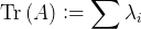$\mathrm{Tr}\,(A) \mathrel{\mathop:}= \sum \lambda _{i}$ when this sum converges absolutely. There is a nice way of calculating the trace: Let $K_{A}\thinspace{:}\thinspace \mathstrut{\Bbb R} ^{n}\times \mathstrut{\Bbb R} ^{n}\rightarrow \mathstrut{\Bbb C} $ be given by $K_{A}(x,\,y) =\sum \lambda _{i}\phi _{i}(x) \overline{\phi _{i}(y) }$ ; then, so long as this sum converges uniformly and absolutely, $K_{A}$ is the integral kernel of A (i.e., for $\psi \in L^{2}(\mathstrut{\Bbb R} ^{n}) $ , $A(\psi) (x) =\int_{\mathstrut{\Bbb R} ^{n}}K_{A}(x,\,y) \psi (y) dy$ ); and in this case 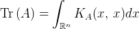$\mathrm{Tr}\,(A) =\int_{\mathstrut{\Bbb R} ^{n}}K_{A}(x,\,x) dx$ . A nice feature of this formula is that the left-hand side is algebraic and the right-hand side is analytic-geometric.

When A has discrete spectrum, but is not of trace class, we can proceed as follows. Let $\varphi \thinspace{:}\thinspace \mathstrut{\Bbb R} \rightarrow \mathstrut{\Bbb R} $ be Schwartz (so that it and all its derivatives decrease rapidly as ∞ is approached), and suppose that $\sum \varphi (\lambda _{i}) $ converges absolutely. Then we switch our attention to the operator $\varphi (A) $ (i.e., that operator with eigenbasis $\{ \phi _{i}\} $ with corresponding eigenvalues $\{ \varphi (\lambda _{i}) \} $ ). This operator is of trace class, with trace given by $\sum \varphi (\lambda _{i}) $ . We can study the integrals $\mathrm{Tr}\,(\varphi (A)) =\int_{\mathstrut{\Bbb R} ^{n}}K_{\varphi (A) }(x,\,x) dx$ . This gives us information about the spectrum of A as we vary ϕ.

Often we are interested in an operator, but we don't have even the most basic knowledge of its spectrum—let alone the sort required to calculate the trace from first principles or via the integral kernel. It turns out, though, that there are expressions which give us semiclassical information about the trace of such operators in terms of certain geometrical structures of the classical theory, without requiring us to have prior knowledge of the eigenfunctions and eigenvalues.

Third Stage: Semiclassical Trace Formulae. I am going to say just a bit about such results—just enough to give you feel for what Batterman is up to.

Here is the central result.Footnote ³¹ Let E be a noncritical value of the classical energy.Footnote ³² Then there exists a sequence $\{ \gamma _{i}\} $ of distributions defined on $\mathstrut{\Bbb R} $ such that for any Schwartz ϕ with compactly supported Fourier transform $\hat{\varphi }$ , we find that as $h\rightarrow \infty $

(Here ε is a constant that depends only upon the Hamiltonian.) This is a sort of semiclassical trace formula—it gives us information about the sum of certain ranges of eigenvalues, as $h\rightarrow \infty $ . The crucial point for our purposes is that the support of each of the distributions $\gamma _{i}$ is contained in the set of periods of the periodic classical trajectories lying on the classical energy surface $H^{-1}(E) $ —in order to calculate with this formula, we need to know about the behavior of classicaltrajectories.

This trace formula is valid for a wide range of systems, regular and chaotic. Now let us assume that the periodic trajectories of the classical flow are nondegenerate—roughly, that within each energy surface they are isolated from one another rather than occurring in continuous families. This condition will obtain in chaotic classical systems. In this case, there is a semiclassical trace formula whose left-hand side is of the above form and whose right-hand side involves a number of terms with a geometrical interpretation—a term involving the Liouville measure induced on the classical energy surface, a sum over the classical periodic trajectories of a function of the classical action, and so on.Footnote ³³

5. Consequences?

The picture that emerges from these examples is described thus by Batterman: “Wave theoretic or quantum mechanical aspects are sewn onto a skeleton of classical trajectories and their structures in the asymptotic … limit” (127). How is this observation supposed to carry us through to the conclusion that wave-theoretic optics and quantum mechanics are explanatorily inadequate—that there are phenomena whose understanding ineliminably involves the concepts of geometric optics and classical mechanics?

Let us explicitly separate two of Batterman's theses. The first thesis is that the successful explanation of a regularly occurring phenomenon involves two tasks: (i) finding solutions to the equations of a given theory that possess a feature corresponding to the occurrence of the phenomenon in question; and (ii) showing (something like) that the possession of this feature is stable under (generic) physically realistic perturbations of such solutions. This thesis seems entirely correct to me—and I think it one of the great virtues of Batterman's work that it calls attention to the mathematical difficulty and philosophical interest of task (ii).Footnote ³⁴

The second thesis, which I think we should reject, is that Batterman's examples provide cases where a given theory contains resources adequate to the first of these explanatory tasks but not to the second—but where both tasks can be accomplished when the resources of the given theory are supplemented by resources of a less fundamental theory. In the case of the rainbow, it is claimed (90-91) that although one can construct solutions to the equations of wave optics corresponding to the appearance of the rainbow, one is unable to show that this behavior is generic within the relevant range of circumstances without recourse to ray-theoretic notions such as caustics. Similarly it is claimed (109-110) that there exist (rather more abstract) quantum mechanical phenomena (involving eigenvalue statistics, etc.) that can be understood only when the resources of quantum mechanics are supplemented by knowledge of the classical mechanical trajectories in phase space. Considering the first example, Batterman asks whether the features of the rainbow that we are interested in—the form of the bow, the interference fringes on its lit side, etc.—can be explained within wave-theoretic optics. His answer:

Batterman thinks that a delicate balance must be struck in considering each of his examples. For the phenomena he is interested in, Batterman locates some of the resources crucial to their explanation in the limiting regime between a more, and a less, fundamental theory. He thinks that while there is some sense in which these resources are contained in the more fundamental theory, there is also a sense in which they are unpredictable from it alone—since “the understanding of those mathematical representations requires reference to structures foreign to the fundamental theory” (96; cf. 109 ff.).

Against this, I claim that an examination of the sense in which rays and caustics are implicit in the apparatus of the wave theory, and of the sense in which classical phase space trajectories are implicit in the mathematical structure of quantum mechanics, saps all intuitive force from Batterman's claim that we here have cases where the understanding of phenomena requires that the resources of the more fundamental theories be supplemented by resources of the less fundamental theories. In brief outline, the argument is as follows. In Batterman's cases, the physics of the more fundamental theory is described by a certain partial differential equation whose independent variables parameterize a manifold X. Suppose that we ask some mathematicians to investigate the asymptotic behavior of approximate solutions to this equation (or the behavior of the spectrum of the corresponding operator) as some parameter appearing in the equation grows large or small. One of the most powerful techniques for attacking such problems involves the construction and investigation of an auxiliary problem definable from knowledge of the original problem. One first constructs a new manifold $T^{*}X$ , the cotangent bundle associated with X (a point of $T^{*}X$ is a pair (x, ξ) consisting of a point $x\in X$ and a covector ξ at x). One also constructs a function, the principal symbol, on $T^{*}X$ associated with the differential operator of the original problem. $T^{*}X$ carries a natural geometrical structure which in concert with the principal symbol determines a set of curves in $T^{*}X$ . The auxiliary problem consists in the study of these curves. Now, formally speaking, our auxiliary problem is a problem in the theory of Hamiltonian systems: $T^{*}X$ can be thought of as the space of possible positions and momenta for a particle living on X, and our curves are the dynamical trajectories for such a particle if the energy of the particle in each state (x, ξ) is just given by the value of the principal symbol at that state. But in order to construct this auxiliary problem, our mathematicians need not have heard of any physical theory (such as classical mechanics), whose mathematics is given by the theory of Hamiltonian systems—the auxiliary problem can be constructed uniquely as soon as the original problem is given, the structures needed to set up the auxiliary problem being definable in terms of those used to set up the original one. And once they have the auxiliary problem at hand, our mathematicians can see that the asymptotic behavior features of the original problem will turn upon the features of the auxiliary problem—in the optics case, in the high frequency limit, approximate solutions to the wave equation blow up near points of X where the projection of certain dynamical trajectories from $T^{*}X$ to X becomes singular (these are the caustic points) while in the quantum mechanics case, periodic dynamical trajectories in the auxiliary problem will play a special role in the analysis of the spectrum of the quantum Hamiltonian in the $h\rightarrow 0$ limit. So there is, as far as the mathematics goes, nothing foreign to the more fundamental theory about the ingredients needed to prove the asymptotic results that secure explanations of phenomena such as the rainbow—these ingredients are implicit in the mathematics of the more fundamental theory.

Two questions remain. (1) How does all of this work? (2) When one tries to understand all of this as physics rather than as mere mathematics, does one have to draw upon the conceptual resources of the less fundamental theory after all? I address these two questions, in turn, in the following subsections. (Readers uninterested in (1) should skip to Section 5.2.)

5.1. More Details

I describe in slightly more detail the construction of the auxiliary problem associated with a given differential equation and its role in the asymptotic investigation of that equation.Footnote ³⁵ Suppose that we are interested in the study of a linear partial differential equation whose independent variables parameterize a manifold X of dimension n. We assume that this differential equation is of order m and depends upon a parameter τ. We suppose that in coordinates we can write the equation in the form $P(x,\,\partial /\partial x,\,\tau) u(x) =0$ , with $u\in C^{\infty }(X) $ and P of the form $P=\sum_{\alpha =0}^{m}a_{\alpha }(x,\,\tau) (\tau (\partial /\partial x)) ^{\alpha }$ with each $a_{\alpha }$ of the form $\sum_{j=0}^{\infty }b_{\alpha,j}(x) \tau ^{j}$ .Footnote ³⁶ Recall that $T^{*}X$ is the cotangent bundle of X—the points (x, ξ) of this space can be thought of as the possible positions and momenta of a particle moving in X. The manifold $T^{*}X$ possesses a natural symplectic structure ω (in virtue of being a cotangent bundle). For present purposes, we can think of ω as being, more or less, an antisymmetric metric on $T^{*}X$ .Footnote ³⁷ We introduce the principal symbol of the operator P: This is the function $P_{0}\thinspace{:}\thinspace T^{*}X\rightarrow \mathstrut{\Bbb R} $ , defined as $P_{0}(x,\,\xi) \mathrel{\mathop:}= \sum b_{\alpha,0}\xi ^{\alpha }$ .Footnote ³⁸

Now, in classical mechanics, if the possible configurations of a physical system are parameterized by a manifold Q (the configuration space), then its possible dynamical states (positions and momenta) are parameterized by the associated cotangent bundle $T^{*}Q$ (the phase space), and the dynamics are determined by specifying a Hamiltonian function, $H\thinspace{:}\thinspace T^{*}Q\rightarrow \mathstrut{\Bbb R} $ , assigning to each dynamical state its total energy. The Hamiltonian encodes information about the forces acting on the system, and in concert with the natural symplectic structure on $T^{*}Q$ , it determines a vector field on $T^{*}Q$ whose integral curves correspond to the dynamical trajectories of the theory.Footnote ³⁹ Without invoking any physical interpretation, we can employ the same mathematics to associate with our principal symbol $P_{0}$ , a vector field $\Xi _{P_{0}}$ , on $T^{*}X$ . The integral curves of this vector field are called the bicharacteristic strips.

So given X and P, we construct $T^{*}X$ , $P_{0}$ , and $\Xi _{P_{0}}$ . The study of the associated bicharacteristic strips is the auxiliary mathematical problem that plays a role in the study of the asymptotic behavior of our original differential equation, $Pu=0$ . The account of the role of this auxiliary problem is somewhat involved. I focus on the construction of approximate solutions in the asymptotic regime, and break the procedure into three steps.

First Step: Find a Lagrangian manifold that solves the Hamilton-Jacobi equation. Because the symplectic form ω on $T^{*}X$ is antisymmetric, if $(x,\,\xi) \in T^{*}X$ and $v\in T_{(x,\xi) }T^{*}X$ , then $\omega (v,\,v) =0$ —i.e., the symplectic product of a tangent vector to $T^{*}X$ with itself always vanishes. But for fixed v in the tangent space at (x, ξ), there will in fact be many w in that tangent space such that $\omega (v,\,w) =0$ . We look for an n-dimensional submanifold L of $T^{*}X$ with the property that at any point of L, any two vectors v and w in the tangent space to L at that point satisfy $\omega (v,\,w) =0$ (n is the maximum possible dimension of such a submanifold). Such an L is called a Lagrangian submanifold. We are looking for a Lagrangian submanifold that satisfies the Hamilton-Jacobi equation—this just means that $P_{0}$ is constant on L.Footnote ⁴⁰

Second Step: Find a function on L invariant under the flow induced by $P_{0}$ . Suppose that we have such a submanifold, L. Our next step in constructing our approximate solution to our equation is to look for a scalar function, α, defined on L with the property that the Lie derivative of α in the direction $\Xi _{P_{0}}$ vanishes.Footnote ⁴¹

Third Step: Project the structure (L, α) down to X. When all goes well, the structure (L, α) can be projected down to X to yield a second-order approximate solution to our differential equation $Pu=0$ .Footnote ⁴² Let $\pi \thinspace{:}\thinspace T^{*}X\rightarrow X$ be the projection map (so $\pi (x,\,\xi) =x$ ). We call a point of L regular if the restriction of π to L is a diffeomorphism on some neighborhood of that point; otherwise we call that point singular. We call the image under π of the bicharacteristic strips the bicharacteristic curves. For any regular point of L there is a sufficiently small neighborhood U, so that the bicharacteristic curves in $\pi (U) $ do not cross; but at the image under π of any singular point of L the bicharacteristic curves will intersect one another. If U is a sufficiently small open set of regular points of L on which π acts as a diffeomorphism, then we can find a function S and a function a (actually a half-density) defined on $\pi (U) \subset X$ such that: (i) $U=\{ (x,\,dS(x)) \thinspace{:}\thinspace x\in \pi (U) \} $ ; and (ii) $a=(dS) ^{*}\alpha $ (that is, we pull α back to X using the one-form dS, thought of as a map from $\pi (U) \subset X$ to $U\subset T^{*}X$ ). So we can break the regular part of L up into subsets, $U_{j}$ , projectable to X, such that the structure (L, α) can be encoded in functions $S_{j}$ and $a_{j}$ living on the $\pi (U_{j}) $ . Roughly speaking, $u(x) =\sum e^{i\tau S_{j}(x) }a_{j}(x) $ is our second-order approximate solution to $Pu=0$ . But we still have subtleties to worry about—the phases of the terms in this sum need to be made to mesh, and we have to take the singular points of L into account. The final upshot is: (i) only certain L will be admissible—that is, embedded in $T^{*}X$ in such a way that the whole process can be carried out consistently; (ii) the final form for an asymptotic solution to $Pu=0$ corresponding to (L, α) will consist of a finite sum of integrals of the form

(where K is a compact subset of $\mathstrut{\Bbb R} ^{k}$ , and the y are to be thought of as auxiliary variables).Footnote ⁴³

What does all this have to do with Batterman's examples? Well, for the differential operator of the reduced wave equation the corresponding principal symbol is the kinetic energy deriving from the metric on X (where here X represents physical space). In this case, the bicharacteristic strips correspond to the geodesic flow on $T^{*}X$ , and their images on X, the bicharacteristic curves, are just the geodesics of X. These last correspond to light rays in the physical situation described by (L, α). The images of the singular points of L under π form the caustic corresponding to this family of rays. It follows from our recipe for pulling back (L, α) to X and from the principle of stationary phase that our approximate solution will have asymptotic behavior at the caustic of the sort we are familiar with from the rainbow case.

In the quantum mechanical case we are interested in the operator corresponding to the time-independent Schrödinger equation—and the corresponding principal symbol is just the classical Hamiltonian. Our recipe for constructing approximate solutions is a generalization of the WKB method, and the admissible Lagrangian submanifolds lie in the level sets corresponding to the points of the spectrum of the quantum Hamiltonian. So the auxiliary mathematical problem coincides with a mathematical treatment of the classical limit of our quantum problem. In this case, the bicharacteristic strips are the classical dynamical trajectories in $T^{*}X$ . So it is no longer so surprising that these play a special role in the asymptotic analysis of the energy spectrum of our quantum system—since they are definable from knowledge of the quantum Hamiltonian alone, and play a key role in available techniques for constructing approximate solutions. Indeed, the proof of the semiclassical trace formula turns upon the ingredients introduced above: continuous superpositions of Hamilton-Jacobi-like solutions, and application of the principle of stationary phase (see Uribe Reference Uribe, Pérez-Esteva and Villegas-Blas2000, 72 ff.).