1 Introduction
In Part I (Dyachenko, Lushnikov & Korotkevich Reference Dyachenko, Lushnikov and Korotkevich2016), we obtained a Stokes wave solution numerically with high precision and analysed that solution using the Padé approximation. We showed a convergence of the Padé approximation of a Stokes wave to a single branch cut per spatial period in the upper complex half-plane
 $\mathbb{C}^{+}$
of the axillary complex variable
 $w$
. In this paper, we formulate the nonlinear integral equation for the jump of the Stokes wave at the branch cut in the physical (first) sheet of the Riemann surface. We show that the Riemann surface of the Stokes wave has an infinite number of sheets, as sketched in figure 1, and study the structure of the singularities in these sheets.
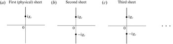
A schematic of Riemann surface sheets for a non-limiting Stokes wave in the complex variable
 ${\it\zeta}$
(1.6) near the origin. The first (physical) sheet (a) has a single square root singularity at
 ${\it\zeta}=\text{i}{\it\chi}_{c}$
in the upper complex half-plane
 $\mathbb{C}^{+}$
with the lower complex half-plane
 $\mathbb{C}^{-}$
corresponding to the domain occupied by the fluid. Other (non-physical) sheets have square root singularities at
 ${\it\zeta}=\pm \text{i}{\it\chi}_{c}$
. Dashed lines show branch cuts. In addition there are the singularities at
 ${\it\zeta}=\pm \text{i}$
in all sheets which corresponds to
 $w=\infty$
. Starting from the third sheet (c) there are square root singularities away from both the real and imaginary axes at distances more that several times
 ${\it\chi}_{c}$
, i.e. well beyond the disks of convergence
 $|{\it\zeta}\pm \text{i}{\it\chi}_{c}|<2{\it\chi}_{c}$
.

A Stokes wave is a fully nonlinear periodic gravity wave propagating with constant velocity
 $c$
(Stokes Reference Stokes1847, Reference Stokes1880a
). It corresponds to two-dimensional potential flow of an ideal incompressible fluid with a free surface. Following Part I (Dyachenko et al.
Reference Dyachenko, Lushnikov and Korotkevich2016), we use scaled units at which
 $c=1$
for the linear gravity waves and the spatial period is
 ${\it\lambda}=2{\rm\pi}$
. Nonlinearity of the Stokes wave increases with an increase of
 $H/{\it\lambda}$
, where
 $H$
is the Stokes wave height which is defined as the vertical distance from the crest to the trough of the Stokes wave. A Stokes wave has
 $c>1$
and the limit
 $H\rightarrow 0,c\rightarrow 1$
corresponds to a linear gravity wave. The Stokes wave of greatest height
 $H=H_{max}$
(also called by the limiting Stokes wave) has a singularity in the form of a sharp angle of
 $2{\rm\pi}/3$
radians on the crest (Stokes Reference Stokes1880b
). We assume that the singularity of the limiting Stokes wave touches the fluid surface at
 $w=0$
and corresponds to the following expansion
 $$\begin{eqnarray}\displaystyle z(w)=\text{i}\frac{c^{2}}{2}-\text{i}\left(\frac{3c}{2}\right)^{2/3}(\text{i}w)^{2/3}+\text{h.o.t.}, & & \displaystyle\end{eqnarray}$$
which ensures the sharp angle of
 $2{\rm\pi}/3$
radians on the crest. Equation (1.1) recovers the result of Stokes (Reference Stokes1880b
). Here h.o.t. means higher-order terms which approach
 $0$
faster than
 $w^{2/3}$
as
 $w\rightarrow 0$
. Also
 $$\begin{eqnarray}\displaystyle z(w)=x(w)+\text{i}y(w) & & \displaystyle\end{eqnarray}$$
is the conformal transformation which maps a half-strip
 $-{\rm\pi}\leqslant u\leqslant {\rm\pi}$
,
 $-\infty <v\leqslant 0$
of the conformal variable
 $$\begin{eqnarray}\displaystyle w=u+\text{i}v & & \displaystyle\end{eqnarray}$$
onto a fluid domain of infinite depth
 $-\infty <y\leqslant {\it\eta}(x),-{\rm\pi}\leqslant x\leqslant {\rm\pi}$
of the complex plane
 $z$
(see Figure 1 of Part I (Dyachenko et al.
Reference Dyachenko, Lushnikov and Korotkevich2016)). Here
 $x$
and
 $y$
are the horizontal and vertical physical coordinates, respectively.
 $y={\it\eta}(x)$
is the surface elevation in the reference frame moving with the speed
 $c$
. As discussed in detail in Part I, choosing
 $$\begin{eqnarray}\displaystyle z(w)=w+\tilde{z}(w), & & \displaystyle\end{eqnarray}$$
with
 $x(w)=u+\tilde{x}(w)$
and
 ${\tilde{y}}(w)=v+y(w)$
, ensures that
 $\tilde{z}(w)$
is
 $2{\rm\pi}$
-periodic function
 $$\begin{eqnarray}\displaystyle \tilde{z}(w+2{\rm\pi})=\tilde{z}(w),\quad \tilde{x}(\pm {\rm\pi})=0. & & \displaystyle\end{eqnarray}$$
It was found by Grant (Reference Grant1973) that the corner singularity (1.1) might not be a simple algebraic branch point because the next-order term in the expansion (1.1) might be a power of the transcendental number. Rigorous results on the asymptotics near the crest of the limiting wave were found in Amick & Fraenkel (Reference Amick and Fraenkel1987), McLeod (Reference McLeod1987). These results were used in Fraenkel (Reference Fraenkel2007), Fraenkel & Harwin (Reference Fraenkel and Harwin2010), Fraenkel (Reference Fraenkel2010) to construct the exact bounds on the limiting Stokes wave and prove the local uniqueness using Banach’s contraction mapping principle. More exact bounds were provided in Tanveer (Reference Tanveer2013). However, the question of whether log terms in the asymptotic expansion are possible in addition to the transcendental power asked in Amick & Fraenkel (Reference Amick and Fraenkel1987) remains open. The existence of a limiting Stokes wave with the jump of the slope at the crest in
 $2{\rm\pi}/3$
radians was independently proven by Amick, Fraenkel & Toland (Reference Amick, Fraenkel and Toland1982) and Plotnikov (Reference Plotnikov1982).
In this paper we focus on analysing singularities of near-limiting Stokes waves. Grant (Reference Grant1973) showed that, assuming that the singularity is a power-law branch point, then that singularity has to have a square root form to the leading order. Tanveer (Reference Tanveer1991) provided a much stronger result proving that the only possible singularity in the finite complex upper half-plane is of a square root type. Plotnikov & Toland (Reference Plotnikov and Toland2002) discusses the existence of a unique square root singularity above crests. The existence of only one square root singularity per period in a finite physical complex plane was also confirmed in Dyachenko, Lushnikov & Korotkevich (Reference Dyachenko, Lushnikov and Korotkevich2013a ) and Part I (Dyachenko et al. Reference Dyachenko, Lushnikov and Korotkevich2016) by analysing the numerical solution for a Stokes wave.
We now consider an additional conformal transformation between the complex plane
 $w=u+\text{i}v$
and the complex plane for the new variable
 $$\begin{eqnarray}\displaystyle {\it\zeta}=\tan \left(\frac{w}{2}\right), & & \displaystyle\end{eqnarray}$$
which maps the strip
 $-{\rm\pi}<\text{Re}(w)<{\rm\pi}$
onto the complex
 ${\it\zeta}$
plane. In particular, the line segment
 $-{\rm\pi}<w<{\rm\pi}$
of the real line
 $w=u$
maps onto the entire real line
 $(-\infty ,\infty )$
in the complex
 ${\it\zeta}$
-plane, as shown in Figure 5 of Part I (Dyachenko et al.
Reference Dyachenko, Lushnikov and Korotkevich2016). Vertical half-lines
 $w=\pm {\rm\pi}+\text{i}v,0<v<\infty$
are mapped onto a branch cut
 $\text{i}<{\it\zeta}<\text{i}\infty$
. In a similar way, vertical half-lines
 $w=\pm {\rm\pi}+\text{i}v,-\infty <v<0$
are mapped onto a branch cut
 $-\text{i}\infty <{\it\zeta}<-\text{i}$
. However, the
 $2{\rm\pi}-$
periodicity of
 $\tilde{z}(w)$
(1.5) allows us to ignore these two branch cuts because
 $\tilde{z}(w)$
is continuous across them. Complex infinities
 $w=\pm \text{i}\infty$
are mapped onto
 ${\it\zeta}=\pm \text{i}$
. An unbounded interval
 $[\text{i}v_{c},\text{i}\infty )$
,
 $v_{c}>0$
is mapped onto a finite interval
 $[\text{i}{\it\chi}_{c},\text{i})$
with
 $$\begin{eqnarray}\displaystyle {\it\chi}_{c}=\tanh \frac{v_{c}}{2}. & & \displaystyle\end{eqnarray}$$
The transformation (1.6) takes care of the
 $2{\rm\pi}-$
periodicity of the Stokes wave so that the function
 $z({\it\zeta})$
defined in the complex plane
 ${\it\zeta}\in \mathbb{C}$
corresponds to the function
 $z(w)$
defined in the strip
 $-{\rm\pi}<\text{Re}(w)=u<{\rm\pi}$
. Here and below we abuse notation and use the same symbol
 $z$
for both functions of
 ${\it\zeta}$
and
 $w$
(and similar for other symbols). The additional advantage of using the mapping (1.6) is the compactness of the interval
 $(\text{i}{\it\chi}_{c},\text{i})$
as mapped from the infinite interval
 $(\text{i}v_{c},\text{i}\infty )$
. Note that the mapping (1.6) is different from the commonly used (see e.g. Schwartz Reference Schwartz1974; Williams Reference Williams1981; Tanveer Reference Tanveer1991) mapping
 ${\it\zeta}=\exp (-\text{i}w)$
(which maps the strip
 $-{\rm\pi}\leqslant \text{Re}(w)<{\rm\pi}$
onto the unit circle). That exponential map leaves the interval
 $(\text{i}v_{c},\text{i}\infty )$
infinite in the
 ${\it\zeta}$
plane.
The main result of this paper is that there are an infinite number of sheets of a Riemann surface with square root branch points located at
 ${\it\zeta}=\pm \text{i}{\it\chi}_{c}$
, starting from the second sheet (the first sheet has a singularity only at
 ${\it\zeta}=\text{i}{\it\chi}_{c}$
). At each sheet (except the first one) these singularities are coupled through complex conjugated terms which appear in the equation for the Stokes wave. In contrast, the only singularity at
 ${\it\zeta}=\text{i}{\it\chi}_{c}$
of the first sheet (besides the singularity at
 ${\it\zeta}=\text{i}$
) does not have a complex conjugated counterpart at
 ${\it\zeta}=-\text{i}{\it\chi}_{c}$
which makes that (physical) sheet distinct from all others. It is conjectured that the leading order form of a non-limiting Stokes wave has the form of an infinite number of nested square root singularities. These nested square roots form a
 $2/3$
power-law singularity of the limiting Stokes wave as
 ${\it\chi}_{c}\rightarrow 0$
.
The paper is organized as follows. In § 2 a closed nonlinear integral equation for a Stokes wave in terms of the density (jump) at the branch cut is derived and the numerical method to solve that integral equation is given. Section 3 provides an alternative form for the equation of a Stokes wave. Section 4 uses that alternative form to find an asymptotic of both a Stokes wave at
 $\text{Im}(w)\rightarrow +\infty$
and the jump at the branch cut. Section 5 discusses a numerical procedure to analyse the structure of the sheets of a Riemann surface for a Stokes wave by the integration of the corresponding nonlinear ordinary differential equation (ODE) in the complex plane. Section 6 derives the analytical expressions for coupled series expansions at
 ${\it\zeta}=\pm \text{i}{\it\chi}_{c}$
to reveal the structure of the Riemann surface for a Stokes wave. Section 7 analyses possible singularities of a Stokes wave in all sheets of a Riemann surface and concludes that the only possible singularity for finite values of
 $w$
is the square root branch point. Section 8 provides a conjecture on recovering of the
 $2/3$
power law of a limiting Stokes wave from an infinite number of nested square root singularities of a non-limiting Stokes wave in the limit
 ${\it\chi}_{c}\rightarrow 0$
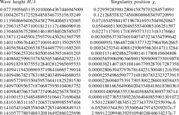
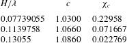
. In § 9 the main results of the paper are discussed. Appendix A shows the equivalence of the two forms of the equation for a Stokes wave used in the main text. Appendix B relates different forms of the equation for Stokes wave in the rest frame and in the moving frame. Appendix C provides tables of the numerical parameters of a Stokes wave.
2 Closed integral equation for a Stokes wave through the density at the branch cut
The equation for a Stokes wave was derived in Zakharov & Dyachenkov (Reference Zakharov and Dyachenkov1996) and Part I (Dyachenko et al.
Reference Dyachenko, Lushnikov and Korotkevich2016) from Euler’s equations for the potential flow of an ideal fluid with a free surface (see also appendices A and B). That equation is defined at the real line
 $w=u$
and takes the following form
 $$\begin{eqnarray}\displaystyle -c^{2}y_{u}+yy_{u}+{\hat{H}}[y(1+\tilde{x}_{u})]=0, & & \displaystyle\end{eqnarray}$$
where
 $$\begin{eqnarray}\displaystyle {\hat{H}}f(u)=\frac{1}{{\rm\pi}}\text{ p.v. }\int _{-\infty }^{+\infty }\frac{f(u^{\prime })}{u^{\prime }-u}\,\text{d}u^{\prime } & & \displaystyle\end{eqnarray}$$
is the Hilbert transform with p.v. meaning a Cauchy principal value of an integral and the subscripts in
 $t$
and
 $u$
mean partial derivatives here and below. The Hilbert operator
 ${\hat{H}}$
transforms into the multiplication operator
 $$\begin{eqnarray}\displaystyle ({\hat{H}}f)_{k}=\text{i}\text{ sign}(k)f_{k}, & & \displaystyle\end{eqnarray}$$
for the Fourier coefficients (harmonics)
 $f_{k}$
,
 $$\begin{eqnarray}\displaystyle f_{k}=\frac{1}{2{\rm\pi}}\int _{-{\rm\pi}}^{{\rm\pi}}f(u)\exp (-\text{i}ku)\,\text{d}u, & & \displaystyle\end{eqnarray}$$
of the periodic function
 $f(u)=f(u+2{\rm\pi})$
represented through the Fourier series
 $$\begin{eqnarray}\displaystyle f(u)=\mathop{\sum }_{k=-\infty }^{\infty }f_{k}\exp (\text{i}ku). & & \displaystyle\end{eqnarray}$$
Here
 $\text{sign}(k)=-1,0,1$
for
 $k<0,k=0$
and
 $k>0$
, respectively. Equation (2.5) implies that
 $$\begin{eqnarray}\displaystyle {\hat{H}}^{2}f=-(f-f_{0}), & & \displaystyle\end{eqnarray}$$
where
 $f_{0}$
is the zeroth Fourier harmonic of
 $f$
.
It is convenient to decompose the Fourier series (2.5) as follows
 $$\begin{eqnarray}\displaystyle f(u)=f^{+}(u)+f^{-}(u)+f_{0}, & & \displaystyle\end{eqnarray}$$
where
 $$\begin{eqnarray}\displaystyle f^{+}(w)=\mathop{\sum }_{k=1}^{\infty }f_{k}\exp (\text{i}kw) & & \displaystyle\end{eqnarray}$$
is the analytical function in
 $\mathbb{C}^{+}$
and
 $$\begin{eqnarray}\displaystyle f^{-}(w)=\mathop{\sum }_{k=-\infty }^{-1}f_{k}\exp (\text{i}kw) & & \displaystyle\end{eqnarray}$$
is the analytical function in the lower complex half-plane
 $\mathbb{C}^{-}$
. Then (2.3) implies that
 $$\begin{eqnarray}\displaystyle {\hat{H}}f=\text{i}(f^{+}-f^{-}). & & \displaystyle\end{eqnarray}$$
Also using (2.3) we define the operator,
 $$\begin{eqnarray}\displaystyle \hat{P}={\textstyle \frac{1}{2}}(1+\text{i}{\hat{H}}), & & \displaystyle\end{eqnarray}$$
projecting any
 $2{\rm\pi}$
-periodic function
 $f$
into a function which has analytical continuation from the real line
 $w=u$
into
 $\mathbb{C}^{-}$
as follows
 $$\begin{eqnarray}\displaystyle \hat{P}f=f^{-}+\frac{f_{0}}{2}. & & \displaystyle\end{eqnarray}$$
One can apply
 ${\hat{H}}$
to (2.1) to obtain the following closed expression for
 $y$
,
 $$\begin{eqnarray}\displaystyle (c^{2}\hat{k}-1)y-\left(\frac{\hat{k}y^{2}}{2}+y\hat{k}y\right)=0, & & \displaystyle\end{eqnarray}$$
where
 $\hat{k}\equiv -\partial _{u}{\hat{H}}=\sqrt{-{\rm\nabla}^{2}}$
and we have used the following relations
 $$\begin{eqnarray}\displaystyle y_{u}={\hat{H}}\tilde{x}_{u}\quad \text{and}\quad \tilde{x}_{u}=-{\hat{H}}y_{u}, & & \displaystyle\end{eqnarray}$$
which are valid for the analytic function
 $\tilde{z}_{u}(w)$
satisfying the decaying condition
 $\tilde{z}_{u}(w)\rightarrow 0$
as
 $v\rightarrow -\infty$
. We also assume in deriving (2.13) from (2.1) that
 $$\begin{eqnarray}\displaystyle \int _{-{\rm\pi}}^{{\rm\pi}}{\it\eta}(x)\,\text{d}x=\int _{-{\rm\pi}}^{{\rm\pi}}y(u)x_{u}(u)\,\text{d}u=0, & & \displaystyle\end{eqnarray}$$
meaning that the mean elevation of the free surface is set to zero. Equation (2.15) reflects the conservation of the total mass of fluid. Equation (2.13) was derived in Babenko (Reference Babenko1987) and later was independently obtained from the results of Dyachenko et al. (Reference Dyachenko, Kuznetsov, Spector and Zakharov1996) in Dyachenko et al. (Reference Dyachenko, Lushnikov and Korotkevich2013a ). See also Zakharov & Dyachenkov (Reference Zakharov and Dyachenkov1996) for a somewhat similar equation. Babenko (Reference Babenko1987) and subsequent developments in Plotnikov (Reference Plotnikov1991), Buffoni, Dancer & Toland (Reference Buffoni, Dancer and Toland2000), Buffoni & Toland (Reference Buffoni and Toland2001), Shargorodsky & Toland (Reference Shargorodsky and Toland2008) used an equation of the type (2.13) for the analysis of bifurcations.
Equation (2.13) is convenient for numerical simulation of a Stokes wave because it depends on
 $y$
only, as detailed in Part I (Dyachenko et al.
Reference Dyachenko, Lushnikov and Korotkevich2016). The operator
 $\hat{k}$
is the multiplication operator in the Fourier domain which is straightforward to evaluate numerically using fast Fourier transform.
In this paper it is however more convenient for our analytical study to rewrite the equation for a Stokes wave in terms of the complex variable
 $\tilde{z}$
. For that, we apply the projector operator
 $\hat{P}$
(2.11) to (2.1) which results in
 $$\begin{eqnarray}\displaystyle c^{2}\tilde{z}_{u}=-\text{i}\hat{P}[(\tilde{z}-\bar{\tilde{z}})(1+\tilde{z}_{u})], & & \displaystyle\end{eqnarray}$$
where
 $\bar{f}(u)\equiv \bar{f}$
means complex conjugation of the function
 $f(u)$
. Note that the complex conjugation
 $\bar{f}(w)$
of
 $f(w)$
in this paper is understood to be applied with the assumption that
 $f(w)$
is the complex-valued function of the real argument
 $w$
even if
 $w$
takes complex values so that
 $$\begin{eqnarray}\displaystyle \bar{f}(w)\equiv \overline{f(\bar{w})}. & & \displaystyle\end{eqnarray}$$
This definition ensures the analytical continuation of
 $f(w)$
from the real axis
 $w=u$
into the complex plane of
 $w\in \mathbb{C}$
and similar for functions of
 ${\it\zeta}\in \mathbb{C}$
. If the function
 $f(w)$
is analytic in
 $\mathbb{C}^{-}$
then
 $\bar{f}(w)$
is analytic in
 $\mathbb{C}^{+}$
, as also follows from (2.7)–(2.9).
A numerical convergence of the Padé approximation to the continuous density
 ${\it\rho}({\it\chi})$
of the branch cut was shown in Part I (Dyachenko et al.
Reference Dyachenko, Lushnikov and Korotkevich2016) together with the parametrization of the branch cut of a Stokes wave, as follows
 $$\begin{eqnarray}\displaystyle \tilde{z}({\it\zeta})=\text{i}y_{b}+\int _{{\it\chi}_{c}}^{1}{\displaystyle \frac{{\it\rho}({\it\chi}^{\prime })\,\text{d}{\it\chi}^{\prime }}{{\it\zeta}-\text{i}{\it\chi}^{\prime }}}, & & \displaystyle\end{eqnarray}$$
where
 $y_{b}\equiv y(u)|_{u=\pm {\rm\pi}}\in \mathbb{R}$
is the minimum height of a Stokes wave as a function of
 $x$
(or in the similar way as the function of
 $u$
). The density
 ${\it\rho}({\it\chi})$
is related to the jump
 ${\rm\Delta}_{jump}$
of
 $\tilde{z}({\it\zeta})$
for crossing the branch cut at
 ${\it\zeta}=\text{i}{\it\chi}$
in a counterclockwise direction as follows
 $$\begin{eqnarray}\displaystyle \tilde{{\rm\Delta}}_{jump}\equiv z({\it\zeta})|_{{\it\zeta}=\text{i}{\it\chi}-0}-\tilde{z}({\it\zeta})|_{{\it\zeta}=\text{i}{\it\chi}+0}=-2{\rm\pi}{\it\rho}({\it\chi}), & & \displaystyle\end{eqnarray}$$
see also Part I (Dyachenko et al.
Reference Dyachenko, Lushnikov and Korotkevich2016) for more details. We now use the parametrization (2.18) to study the Stokes wave equation (2.16). We eliminate the constant
 $\text{i}y_{b}$
at
 ${\it\zeta}=\infty$
in (2.18) by introducing a new function
 $$\begin{eqnarray}\displaystyle f(u)=\tilde{z}(u)-\text{i}y_{b}=\int _{{\it\chi}_{c}}^{1}{\displaystyle \frac{{\it\rho}({\it\chi}^{\prime })\,\text{d}{\it\chi}^{\prime }}{{\it\zeta}-\text{i}{\it\chi}^{\prime }}}, & & \displaystyle\end{eqnarray}$$
together with the complex conjugate
 $$\begin{eqnarray}\displaystyle \bar{f}(u)=\int _{{\it\chi}_{c}}^{1}{\displaystyle \frac{{\it\rho}({\it\chi}^{\prime })\,\text{d}{\it\chi}^{\prime }}{{\it\zeta}+\text{i}{\it\chi}^{\prime }}}, & & \displaystyle\end{eqnarray}$$
which was evaluated using the definition (2.17).
Equation (2.16) in the new variable (2.20) takes the following form
 $$\begin{eqnarray}\displaystyle -\text{i}c^{2}f_{u}+\text{i}y_{b}+2\text{i}y_{b}f_{u}+ff_{u}+\hat{P}f-\hat{P}\bar{f}-\hat{P}[\bar{f}f_{u}]=0, & & \displaystyle\end{eqnarray}$$
with
 $f$
and
 $\bar{f}$
given by (2.20) and (2.21), respectively.
2.1 Projection in the
 ${\it\zeta}$
plane

The projector
 $\hat{P}$
(2.11) is defined in terms of the independent variable
 $u$
. Using (2.22), together with the definition (2.20), suggests a switch from
 $u$
into the independent variable
 ${\it\zeta}$
. To identify how to compute
 $\hat{P}$
in the complex
 ${\it\zeta}$
-plane, we start from the Fourier series (2.4), (2.7) in variable
 $u$
and make a change of variable (1.6) (assuming that
 $-{\rm\pi}\leqslant u\leqslant {\rm\pi}$
and
 ${\it\zeta}\in \mathbb{R}$
) as follows
 $$\begin{eqnarray}\displaystyle f(u)=f({\it\zeta})=\mathop{\sum }_{k=-\infty }^{\infty }f_{n}\text{e}^{\text{i}ku}=\mathop{\sum }_{k=-\infty }^{\infty }f_{n}\exp [2\text{i}k\arctan {\it\zeta}]=\mathop{\sum }_{n=-\infty }^{\infty }f_{k}\left(\frac{{\it\zeta}-\text{i}}{{\it\zeta}+\text{i}}\right)^{k}(-1)^{k},\quad & & \displaystyle\end{eqnarray}$$
where we abuse notation by assuming that
 $\tilde{f}({\it\zeta})\equiv f(u)$
and removing
 $\tilde{\text{}}$
sign. Equations (2.11), (2.12) and (2.23) imply that
 $\hat{P}$
removes all Fourier harmonics with positive
 $n$
and replaces the zeroth harmonic
 $f_{0}$
by
 $f_{0}/2$
as follows
 $$\begin{eqnarray}\displaystyle \hat{P}f(u)=\mathop{\sum }_{n=-\infty }^{\infty }f_{k}\hat{P}\text{e}^{\text{i}ku} & = & \displaystyle \frac{f_{0}}{2}+\mathop{\sum }_{k=-\infty }^{-1}f_{k}\exp [\text{i}k2\arctan {\it\zeta}]\nonumber\\ \displaystyle & = & \displaystyle \frac{f_{0}}{2}+\mathop{\sum }_{n=-\infty }^{-1}f_{k}\left(\frac{{\it\zeta}-\text{i}}{{\it\zeta}+\text{i}}\right)^{k}(-1)^{k}.\end{eqnarray}$$
Consider a particular case
 $f(u)=1/({\it\zeta}-\text{i}{\it\chi})$
,
 ${\it\chi}\in \mathbb{R}$
and
 ${\it\chi}\neq 0$
. We calculate
 $f_{k}$
by (2.4) and (2.23) through the change of variable (1.6) implying
 $\text{d}u=2/({\it\zeta}^{2}+1)\,\text{d}{\it\zeta}$
as follows
 $$\begin{eqnarray}\displaystyle f_{-k}=\frac{1}{2{\rm\pi}}\int _{-{\rm\pi}}^{{\rm\pi}}f(u)\text{e}^{\text{i}ku}\,\text{d}u=\frac{1}{2{\rm\pi}}\int _{-\infty }^{\infty }\frac{1}{{\it\zeta}-\text{i}{\it\chi}}\left(\frac{{\it\zeta}-\text{i}}{{\it\zeta}+\text{i}}\right)^{k}(-1)^{k}\frac{2}{{\it\zeta}^{2}+1}\,\text{d}{\it\zeta}. & & \displaystyle\end{eqnarray}$$
Assuming
 $k\geqslant 0$
and closing the complex integration contour in the upper half-plane of
 ${\it\zeta}$
we obtain that
 $$\begin{eqnarray}\displaystyle f_{-k}=\text{i}\left(\frac{{\it\chi}-1}{{\it\chi}+1}\right)^{k}(-1)^{k}\frac{2}{-{\it\chi}^{2}+1}{\it\theta}({\it\chi})+{\it\delta}_{k,0}\frac{1}{\text{i}-\text{i}{\it\chi}}. & & \displaystyle\end{eqnarray}$$
For the zeroth harmonic
 $f_{0}$
, (2.26) results in
 $$\begin{eqnarray}\displaystyle f_{0}=\frac{\text{i}\text{ sign}({\it\chi})}{1+{\it\chi}\text{ sign}({\it\chi})}, & & \displaystyle\end{eqnarray}$$
where
 $\text{sign}({\it\chi})=1$
for
 ${\it\chi}>0$
and
 $\text{sign}({\it\chi})=-1$
for
 ${\it\chi}<0$
.
Using now (2.24), (2.26) and (2.27) we find that
 $$\begin{eqnarray}\displaystyle \hat{P}\frac{1}{{\it\zeta}-\text{i}{\it\chi}} & = & \displaystyle \frac{-\text{i}\text{ sign}({\it\chi})}{2[1+{\it\chi}\text{ sign}({\it\chi})]}+\mathop{\sum }_{k=0}^{\infty }\left[\text{i}\left(\frac{{\it\chi}-1}{{\it\chi}+1}\right)^{k}(-1)^{k}\frac{2}{-{\it\chi}^{2}+1}{\it\theta}({\it\chi})+{\it\delta}_{k,0}\frac{1}{\text{i}-\text{i}{\it\chi}}\right]\nonumber\\ \displaystyle & & \displaystyle \times \,\left(\frac{{\it\zeta}+\text{i}}{{\it\zeta}-\text{i}}\right)^{k}(-1)^{k}=\frac{1}{{\it\zeta}-\text{i}{\it\chi}}{\it\theta}({\it\chi})+\frac{1}{\text{i}-\text{i}{\it\chi}}{\it\theta}(-{\it\chi})-\frac{\text{i}\text{ sign}({\it\chi})}{2[1+{\it\chi}\text{ sign}({\it\chi})]},\nonumber\\ \displaystyle & & \displaystyle\end{eqnarray}$$
where
 ${\it\theta}({\it\chi})=1$
for
 ${\it\chi}>0$
and
 ${\it\theta}({\it\chi})=0$
for
 ${\it\chi}<0$
.
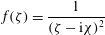
In a similar way, for
 $f({\it\zeta})={\displaystyle \frac{1}{({\it\zeta}-\text{i}{\it\chi})^{2}}}$
we find from the series (2.23) that
 $$\begin{eqnarray}\displaystyle f_{-k}=\frac{1}{2{\rm\pi}}\int _{-\infty }^{\infty }\frac{1}{({\it\zeta}-\text{i}{\it\chi})^{2}}\left(\frac{{\it\zeta}-\text{i}}{{\it\zeta}+\text{i}}\right)^{k}(-1)^{k}\frac{2}{{\it\zeta}^{2}+1}\,\text{d}{\it\zeta},\quad k\geqslant 0. & & \displaystyle\end{eqnarray}$$
Closing the complex integration contour in the upper half-plane of
 ${\it\zeta}$
one obtains from (2.29) that
 $$\begin{eqnarray}\displaystyle f_{-k}=\left.\text{i}\frac{\text{d}}{\text{d}{\it\zeta}}\left(\frac{{\it\zeta}-\text{i}}{{\it\zeta}+\text{i}}\right)^{k}(-1)^{k}\frac{2}{{\it\zeta}^{2}+1}{\it\theta}({\it\chi})\right|_{{\it\zeta}=i{\it\chi}}+{\it\delta}_{k,0}\frac{1}{(\text{i}-\text{i}{\it\chi})^{2}},\quad k\geqslant 0 & & \displaystyle\end{eqnarray}$$
and
 $$\begin{eqnarray}\displaystyle f_{0}=-\frac{1}{[1+{\it\chi}\text{ sign}({\it\chi})]^{2}}. & & \displaystyle\end{eqnarray}$$
Taking a sum over
 $k$
in (2.24) using (2.30) and (2.31) we find that
 $$\begin{eqnarray}\displaystyle \hat{P}{\displaystyle \frac{1}{({\it\zeta}-\text{i}{\it\chi})^{2}}}=\frac{1}{({\it\zeta}-\text{i}{\it\chi})^{2}}{\it\theta}({\it\chi})+\frac{1}{(\text{i}-\text{i}{\it\chi})^{2}}{\it\theta}(-{\it\chi})+\frac{1}{2[1+{\it\chi}\text{ sign}({\it\chi})]^{2}}. & & \displaystyle\end{eqnarray}$$
2.2 Integral representation of the equation for a Stokes wave
Using (2.20), (2.28) and (2.32) we obtain the following projections in terms of
 ${\it\rho}({\it\chi})$
:
 $$\begin{eqnarray}\displaystyle \hat{P}f=\int _{{\it\chi}_{c}}^{1}{\displaystyle \frac{{\it\rho}({\it\chi})\,\text{d}{\it\chi}}{{\it\zeta}-\text{i}{\it\chi}}}-\int _{{\it\chi}_{c}}^{1}\frac{\text{i}{\it\rho}({\it\chi})\,\text{d}{\it\chi}}{2(1+{\it\chi})},\quad \hat{P}\bar{f}=-\int _{{\it\chi}_{c}}^{1}{\displaystyle \frac{\text{i}{\it\rho}({\it\chi})\,\text{d}{\it\chi}}{2(1+{\it\chi})}}. & & \displaystyle\end{eqnarray}$$
We now find
 $\hat{P}[\bar{f}f_{u}]$
used in (2.22). Equation (1.6) results in the following expression
 $$\begin{eqnarray}\displaystyle \bar{f}f_{u}=\frac{{\it\zeta}^{2}+1}{2}\bar{f}f_{{\it\zeta}}=-\frac{{\it\zeta}^{2}+1}{2}\int _{{\it\chi}_{c}}^{1}\int _{{\it\chi}_{c}}^{1}{\displaystyle \frac{{\it\rho}({\it\chi}^{\prime }){\it\rho}({\it\chi}^{\prime \prime })\,\text{d}{\it\chi}^{\prime }\,\text{d}{\it\chi}^{\prime \prime }}{({\it\zeta}+\text{i}{\it\chi}^{\prime })({\it\zeta}-\text{i}{\it\chi}^{\prime \prime })^{2}}}. & & \displaystyle\end{eqnarray}$$
We perform the partial fraction decomposition of the integrand of (2.34) as follows
 $$\begin{eqnarray}\displaystyle -{\displaystyle \frac{{\it\zeta}^{2}+1}{2({\it\zeta}+\text{i}{\it\chi}^{\prime })({\it\zeta}-\text{i}{\it\chi}^{\prime \prime })^{2}}} & = & \displaystyle {\displaystyle \frac{1}{{\it\zeta}+\text{i}{\it\chi}^{\prime }}}{\displaystyle \frac{1-{{\it\chi}^{\prime }}^{2}}{2({\it\chi}^{\prime }+{\it\chi}^{\prime \prime })^{2}}}+{\displaystyle \frac{1}{{\it\zeta}-\text{i}{\it\chi}^{\prime \prime }}}{\displaystyle \frac{-1-2{\it\chi}^{\prime }{\it\chi}^{\prime \prime }-{{\it\chi}^{\prime \prime }}^{2}}{2({\it\chi}^{\prime }+{\it\chi}^{\prime \prime })^{2}}}\nonumber\\ \displaystyle & & \displaystyle +\,{\displaystyle \frac{1}{({\it\zeta}-\text{i}{\it\chi}^{\prime \prime })^{2}}}{\displaystyle \frac{\text{i}(1-{{\it\chi}^{\prime \prime }}^{2})}{2({\it\chi}^{\prime }+{\it\chi}^{\prime \prime })}}.\end{eqnarray}$$
and apply the projector
 $\hat{P}$
to (2.35) which gives, with the use of (2.28) and (2.32), the following expression:
 $$\begin{eqnarray}\displaystyle \hat{P}[\bar{f}\,f_{u}] & = & \displaystyle \int _{{\it\chi}_{c}}^{1}\int _{{\it\chi}_{c}}^{1}\left[{\displaystyle \frac{1}{\text{i}+\text{i}{\it\chi}^{\prime }}}{\displaystyle \frac{1-{{\it\chi}^{\prime }}^{2}}{4({\it\chi}^{\prime }+{\it\chi}^{\prime \prime })^{2}}}+\left({\displaystyle \frac{1}{{\it\zeta}-\text{i}{\it\chi}^{\prime \prime }}}-{\displaystyle \frac{\text{i}}{2(1+{\it\chi}^{\prime \prime })}}\right){\displaystyle \frac{-1-2{\it\chi}^{\prime }{\it\chi}^{\prime \prime }-{{\it\chi}^{\prime \prime }}^{2}}{2({\it\chi}^{\prime }+{\it\chi}^{\prime \prime })^{2}}}\right.\nonumber\\ \displaystyle & & \displaystyle +\,\left.\left({\displaystyle \frac{1}{({\it\zeta}-\text{i}{\it\chi}^{\prime \prime })^{2}}}+{\displaystyle \frac{1}{2(1+{\it\chi}^{\prime \prime })^{2}}}\right){\displaystyle \frac{\text{i}(1-{{\it\chi}^{\prime \prime }}^{2})}{2({\it\chi}^{\prime }+{\it\chi}^{\prime \prime })}}\right]{\it\rho}({\it\chi}^{\prime }){\it\rho}({\it\chi}^{\prime \prime })\,\text{d}{\it\chi}^{\prime }\,\text{d}{\it\chi}^{\prime \prime }.\end{eqnarray}$$
The other nonlinear term in (2.22) has the following integral form
 $$\begin{eqnarray}\displaystyle ff_{u}=\frac{1}{2}(1+{\it\zeta}^{2})ff_{{\it\zeta}}=-\frac{1}{2}(1+{\it\zeta}^{2})\int _{{\it\chi}_{c}}^{1}{\displaystyle \frac{{\it\rho}({\it\chi}^{\prime })\,\text{d}{\it\chi}^{\prime }}{({\it\zeta}-\text{i}{\it\chi}^{\prime })}}\int _{{\it\chi}_{c}}^{1}{\displaystyle \frac{{\it\rho}({\it\chi}^{\prime \prime })\,\text{d}{\it\chi}^{\prime \prime }}{({\it\zeta}-\text{i}{\it\chi}^{\prime \prime })^{2}}}. & & \displaystyle\end{eqnarray}$$
The constant
 $y_{b}$
is determined from (2.15) as follows
 $$\begin{eqnarray}\displaystyle \int _{-{\rm\pi}}^{{\rm\pi}}y(1+\tilde{x}_{u})\,\text{d}u=\int _{-\infty }^{\infty }\left[y_{b}+\frac{(f-\bar{f})}{2\text{i}}\right]\left[1+\frac{(1+{\it\zeta}^{2})}{4}(f_{{\it\zeta}}+\bar{f}_{{\it\zeta}})\right]\frac{2\text{d}{\it\zeta}}{1+{\it\zeta}^{2}}=0, & & \displaystyle\end{eqnarray}$$
which results in, using (2.20), the following equation,
 $$\begin{eqnarray}\displaystyle y_{b}=-\int _{{\it\chi}_{c}}^{1}\int _{{\it\chi}_{c}}^{1}\frac{{\it\rho}({\it\chi}^{\prime }){\it\rho}({\it\chi}^{\prime \prime })\,\text{d}{\it\chi}^{\prime }\,\text{d}{\it\chi}^{\prime \prime }}{2({\it\chi}^{\prime }+{\it\chi}^{\prime \prime })^{2}}-\int _{{\it\chi}_{c}}^{1}\frac{{\it\rho}({\it\chi}^{\prime })\,\text{d}{\it\chi}^{\prime }}{1+{\it\chi}^{\prime }}. & & \displaystyle\end{eqnarray}$$
Equation (2.39) allows us to find
 $y_{b}$
from a given
 ${\it\rho}({\it\chi}).$
This equation also provides a convenient tool to estimate the accuracy of recovering
 ${\it\rho}({\it\chi})$
by the Padé approximation. For that, one compares the numerical value of
 $y_{b}$
obtained from the Stokes solution in Part I (Dyachenko et al.
Reference Dyachenko, Lushnikov and Korotkevich2016) with the result of the direct numerical calculation of right-hand side of (2.39) with
 ${\it\rho}({\it\chi})$
obtained from the Padé approximation in Part I (all of these numerical values are given in tables of Part I (Dyachenko et al.
Reference Dyachenko, Lushnikov and Korotkevich2016), through the electronic attachment to Dyachenko, Lushnikov & Korotkevich (Reference Dyachenko, Lushnikov and Korotkevich2015a
) and at the web link Dyachenko, Lushnikov & Korotkevich (Reference Dyachenko, Lushnikov and Korotkevich2015b
)).
Integrating (2.20) in
 $u$
over the
 $2{\rm\pi}$
-period one obtains the zero Fourier harmonic
 $y_{0}$
of
 $y(u)$
as follows
 $$\begin{eqnarray}\displaystyle y_{0}=y_{b}+\int _{{\it\chi}_{c}}^{1}\frac{{\it\rho}({\it\chi}^{\prime })\,\text{d}{\it\chi}^{\prime }}{1+{\it\chi}^{\prime }}. & & \displaystyle\end{eqnarray}$$
Requiring that (2.20)–(2.22), (2.33), (2.36), (2.37) and (2.39) are satisfied for
 $-\infty <{\it\zeta}<\infty$
, we obtain a system of equations to find the density
 ${\it\rho}({\it\chi})$
along the branch cut for each
 $c$
. That system has a form of nonlinear integral equation for the unknown function
 ${\it\rho}({\it\chi})$
. Taking the limit
 ${\it\zeta}\rightarrow \infty$
in that system results in the following compact expression
 $$\begin{eqnarray}\displaystyle & & \displaystyle \frac{c^{2}}{2}\int _{{\it\chi}_{c}}^{1}{\it\rho}({\it\chi}^{\prime })\,\text{d}{\it\chi}^{\prime }+2\left[-\int _{{\it\chi}_{c}}^{1}\int _{{\it\chi}_{c}}^{1}\frac{{\it\rho}({\it\chi}^{\prime }){\it\rho}({\it\chi}^{\prime \prime })\,\text{d}{\it\chi}^{\prime }\,\text{d}{\it\chi}^{\prime \prime }}{2({\it\chi}^{\prime }+{\it\chi}^{\prime \prime })^{2}}-\int _{{\it\chi}_{c}}^{1}\frac{{\it\rho}({\it\chi}^{\prime })\,\text{d}{\it\chi}^{\prime }}{1+{\it\chi}^{\prime }}\right]\nonumber\\ \displaystyle & & \displaystyle \quad \times \,\left[1-\frac{1}{2}\int _{{\it\chi}_{c}}^{1}{\it\rho}({\it\chi}^{\prime \prime \prime })\,\text{d}{\it\chi}^{\prime \prime \prime }\right]+\int _{{\it\chi}_{c}}^{1}\frac{{\it\rho}({\it\chi}^{\prime })\,\text{d}{\it\chi}^{\prime }}{1+{\it\chi}^{\prime }}\nonumber\\ \displaystyle & & \displaystyle \quad +\,\int _{{\it\chi}_{c}}^{1}\int _{{\it\chi}_{c}}^{1}\frac{(1-{\it\chi}^{\prime }){\it\rho}({\it\chi}^{\prime }){\it\rho}({\it\chi}^{\prime \prime })\,\text{d}{\it\chi}^{\prime }\,\text{d}{\it\chi}^{\prime \prime }}{2({\it\chi}^{\prime }+{\it\chi}^{\prime \prime })^{2}}=0,\end{eqnarray}$$
which can be used to find
 $c$
from a given
 ${\it\rho}({\it\chi})$
.
2.3 Numerical solution for Stokes wave based on the integral representation
To solve the system (2.20)–(2.22), (2.33), (2.36), (2.37) and (2.39) numerically we use the approximation of the integral in (2.18) by the following numerical quadrature
 $$\begin{eqnarray}\displaystyle f(u)=\tilde{z}({\it\zeta})-\text{i}y_{b}=\int _{{\it\chi}_{c}}^{1}{\displaystyle \frac{{\it\rho}({\it\chi}^{\prime })\,\text{d}{\it\chi}^{\prime }}{{\it\zeta}-\text{i}{\it\chi}^{\prime }}}\simeq \mathop{\sum }_{j=1}^{N}{\displaystyle \frac{{\it\gamma}_{j}}{{\it\zeta}-\text{i}{\it\chi}_{j}}}, & & \displaystyle\end{eqnarray}$$
which has a form of the Padé approximation at the discrete set of points
 ${\it\chi}_{c}<{\it\chi}_{1}<{\it\chi}_{2}<\cdots <{\it\chi}_{N}<1$
with weights
 ${\it\gamma}_{j},j=1,2,\ldots ,N$
. Then, the analysis of §§ 2.1 and 2.2 with (2.18) replaced by the approximation (2.42) is carried out in exactly the same way as in (2.20)–(2.39) with each time
 ${\it\rho}({\it\chi})\,\text{d}{\it\chi}$
and
 ${\it\chi}$
replaced by
 ${\it\gamma}_{j}$
and
 ${\it\chi}_{j}$
, respectively. Also the integrals are replaced by summations. It results in the discrete versions of these equations including
 $$\begin{eqnarray}\displaystyle \hat{P}f=\mathop{\sum }_{j=1}^{N}{\displaystyle \frac{{\it\gamma}_{j}}{{\it\zeta}-\text{i}{\it\chi}}}-\mathop{\sum }_{j=1}^{N}\frac{\text{i}{\it\gamma}_{j}}{2(1+{\it\chi})},\quad \hat{P}\bar{f}=-\mathop{\sum }_{j=1}^{N}{\displaystyle \frac{\text{i}{\it\gamma}_{j}}{2(1+{\it\chi})}}, & & \displaystyle\end{eqnarray}$$
 $$\begin{eqnarray}\displaystyle ff_{u}=-\frac{1}{2}(1+{\it\zeta}^{2})\mathop{\sum }_{j^{\prime }=1}^{N}{\displaystyle \frac{{\it\gamma}_{j^{\prime }}}{({\it\zeta}-\text{i}{\it\chi}_{j^{\prime }})}}\mathop{\sum }_{j^{\prime \prime }=1}^{N}{\displaystyle \frac{{\it\gamma}_{j^{\prime \prime }}}{({\it\zeta}-\text{i}{\it\chi}_{j^{\prime \prime }})^{2}}} & & \displaystyle\end{eqnarray}$$
and
 $$\begin{eqnarray}\displaystyle \hat{P}[\bar{f}\,f_{u}] & = & \displaystyle \mathop{\sum }_{j^{\prime }=1}^{N}\mathop{\sum }_{j^{\prime \prime }=1}^{N}\left[{\displaystyle \frac{1}{\text{i}+\text{i}{\it\chi}_{j^{\prime }}}}{\displaystyle \frac{1-{\it\chi}_{j^{\prime }}^{2}}{4({\it\chi}_{j^{\prime }}+{\it\chi}_{j^{\prime \prime }})^{2}}}+\left({\displaystyle \frac{1}{{\it\zeta}-\text{i}{\it\chi}_{j^{\prime \prime }}}}-{\displaystyle \frac{\text{i}}{2(1+{\it\chi}_{j^{\prime \prime }})}}\right)\right.\nonumber\\ \displaystyle & & \displaystyle \times \,\left.{\displaystyle \frac{-1-2{\it\chi}_{j^{\prime }}{\it\chi}_{j^{\prime \prime }}-{\it\chi}_{j^{\prime \prime }}^{2}}{2({\it\chi}_{j^{\prime }}+{\it\chi}_{j^{\prime \prime }})^{2}}}+\left({\displaystyle \frac{1}{({\it\zeta}-\text{i}{\it\chi}_{j^{\prime \prime }})^{2}}}+{\displaystyle \frac{1}{2(1+{\it\chi}_{j^{\prime \prime }})^{2}}}\right){\displaystyle \frac{\text{i}(1-{\it\chi}_{j^{\prime \prime }}^{2})}{2({\it\chi}_{j^{\prime }}+{\it\chi}_{j^{\prime \prime }})}}\right]{\it\gamma}_{j^{\prime }}{\it\gamma}_{j^{\prime \prime }}.\nonumber\\ \displaystyle & & \displaystyle\end{eqnarray}$$
Also (2.39) is replaced in the same discrete approximation by the following equation
 $$\begin{eqnarray}\displaystyle y_{b}=-\mathop{\sum }_{j^{\prime }=1}^{N}\mathop{\sum }_{j^{\prime \prime }=1}^{N}\frac{{\it\gamma}_{j^{\prime }}{\it\gamma}_{j^{\prime \prime }}}{2({\it\chi}_{j^{\prime }}+{\it\chi}_{j^{\prime \prime }})^{2}}-\mathop{\sum }_{j^{\prime }=1}^{N}\frac{{\it\gamma}_{j^{\prime }}}{1+{\it\chi}_{j^{\prime }}}. & & \displaystyle\end{eqnarray}$$
Choosing numerical values
 ${\it\gamma}_{j},{\it\chi}_{j},j=1,2,\ldots ,N$
from the Padé approximants of Part I (Dyachenko et al.
Reference Dyachenko, Lushnikov and Korotkevich2016) (these approximants are also available through the electronic attachment to Dyachenko et al. (Reference Dyachenko, Lushnikov and Korotkevich2015a
) and at the web link Dyachenko et al. (Reference Dyachenko, Lushnikov and Korotkevich2015b
)) we checked that (2.22) (together with (2.43)–(2.46)) is valid for each value of
 $H/{\it\lambda}$
with the same numerical precision as the precision (at least
 $10^{-26}$
) of the Stokes solutions of Part I (Dyachenko et al.
Reference Dyachenko, Lushnikov and Korotkevich2016). Values of
 $N$
in Part I range between tenths for moderates values of
 $H/{\it\lambda}$
up to
 $N=92$
for the highest Stokes wave considered (given by table 4 in Part I (Dyachenko et al.
Reference Dyachenko, Lushnikov and Korotkevich2016)). These moderate numbers are in sharp contrast with the large number
 $M$
of Fourier modes required for constructing these solutions with the same precision (
 $M\simeq 1.3\cdot 10^{8}$
for the highest Stokes wave considered in table 4 of Part I). An explanation for this dramatic difference between required numerical values of
 $M$
and
 $N$
follows from Part I. It was found in Part I that the error of the Fourier method scales as
 $\propto \exp (-2{\it\chi}_{c}M)$
while the error for the Padé approximation of Part I scales as
 $\propto \exp (-c_{1}{\it\chi}_{c}^{1/6}M),c_{1}\sim 1$
. This suggests that solving (2.22), (2.43)–(2.46) for numerical values of
 ${\it\gamma}_{j},{\it\chi}_{j},j=1,2,\ldots ,N$
is an attractive alternative to the numerical methods of Part I.
To solve (2.22), (2.43)–(2.46) numerically, we aim to approximately satisfy (2.22) at the discrete set of points
 $-\infty <{\it\zeta}={\it\zeta}_{i}<\infty ,i=1,2,\ldots ,M_{1}$
. This results in a nonlinear algebraic system of equations to find
 ${\it\gamma}_{j},{\it\chi}_{j},j=1,2,\ldots ,N$
. This system is overdetermined (see e.g. Wilkening & Yu (Reference Wilkening and Yu2012) for an example of using of overdetermined systems for simulating water waves) provided we choose
 $M_{1}>2N$
but it can be solved in the least square sense (by minimizing the sum of squares of the left-hand side of (2.22) taken over points
 ${\it\zeta}={\it\zeta}_{i},i=1,2,\ldots ,M_{1}$
). However, the difficulty in such a straightforward approach is in the extreme ill conditioning of the resulting algebraic system, mainly because of the denominators containing large powers of
 ${\it\chi}_{j}$
which are clearly seen if we try to bring (2.22) to the common denominator. We bypass this difficulty here by providing the explicit procedure to find the appropriate values of
 ${\it\chi}_{j},j=1,2,\ldots ,N$
for each
 ${\it\chi}_{c}$
(see the description of that procedure below in this section) and only after that do we solve (2.22), (2.43)–(2.46) for the unknowns
 ${\it\gamma}_{j},j=1,2,\ldots ,N$
at the discrete set of points
 $-\infty <{\it\zeta}={\it\zeta}_{i}<\infty ,i=1,2,\ldots ,M_{1}.$
Then, the resulting system is the cubic polynomial in
 ${\it\gamma}_{j},~j=1,2,\ldots ,N$
. That system is still moderately ill conditioned but this difficulty is easily overcome by choosing
 $M_{1}$
large enough, with Newton’s iterations used to find numerical values of
 ${\it\gamma}_{j},j=1,2,\ldots ,N$
, thus forming a least square Newton (LSN) algorithm. For example, for
 $H/{\it\lambda}=0.1387112446\ldots$
(corresponding to
 ${\it\chi}_{c}=3.0056373876\ldots \times 10^{-3}$
, see also table 1 of appendix C for details on numerical Stokes waves) we found that it is sufficient to use
 $M_{1}=800$
and
 $N=51$
to achieve
 $10^{-19}$
accuracy for a Stokes wave. For steeper Stokes waves with
 $H/{\it\lambda}=0.1401109676\ldots$
(
 ${\it\chi}_{c}=6.99513864872\ldots \times 10^{-4}$
) and
 $H/{\it\lambda}=0.1408682599\ldots$
(
 ${\it\chi}_{c}=5.6590609636\ldots \times 10^{-5}$
) we found that using
 $M_{1}=1600,N=61$
and
 $M_{1}=10^{4},N=78$
allows us to achieve
 $10^{-18}$
and
 $10^{-19}$
accuracy, respectively. Here values of
 $N$
were chosen to be the same as for the respective Stokes wave in Part I while
 $M_{1}$
is smaller by a factor
 ${\sim}80$
than
 $M=65536$
in the first case and by a factor
 ${\sim}200$
smaller than
 $M=2\,097\,152$
in the third case (values of
 $M$
are given in Part I, through the electronic attachment to Dyachenko et al. (Reference Dyachenko, Lushnikov and Korotkevich2015a
) and at the web link Dyachenko et al. (Reference Dyachenko, Lushnikov and Korotkevich2015b
)). In these examples, using the symmetry of the Stokes wave, the points
 ${\it\zeta}_{j}$
were chosen to have non-negative values, with the first 300 points uniformly spaced as
 ${\it\zeta}_{i}=(i-1)2{\rm\pi}/M$
,
 $i=1,\ldots ,300$
and the remaining
 $M_{1}-300$
points uniformly (in
 $u$
) spanning the remaining interval of positive values of
 ${\it\zeta}$
. After values of
 ${\it\gamma}_{j},j=1,2,\ldots ,N$
are found from the LSN algorithm, (2.42) provides the Padé approximation for the Stokes wave at the entire real line of
 ${\it\zeta}$
. Then, one can use the results of § 6.1 to find the high precision numerical approximation of
 ${\it\chi}_{c}$
, which completes the current step in
 $H/{\it\lambda}$
(or equivalently the current step in
 ${\it\chi}_{c}$
). These steps are repeated to gradually increase
 $H/{\it\lambda}$
(or equivalently decrease
 ${\it\chi}_{c}$
) by changing the velocity parameter
 $c$
to span the desired range of Stokes waves.
The procedure to find the grid
 ${\it\chi}_{j},j=1,2,\ldots ,N$
at each step is the following. Assume that
 ${\it\chi}_{c}<{\it\chi}_{1}<{\it\chi}_{2}<\cdots {\it\chi}_{N-1}<{\it\chi}_{N}<1$
and
 ${\it\chi}_{c}\ll 1$
. We use the property of the Stokes wave that
 ${\it\rho}({\it\chi})$
changes a little with a change of
 $H/{\it\lambda}$
for
 ${\it\chi}\gg {\it\chi}_{c}$
provided
 ${\it\chi}_{c}\ll 1$
. This implies that
 ${\it\chi}_{j}$
can be chosen independently of
 ${\it\chi}_{c}$
for all
 $j$
such that
 ${\it\chi}_{j}\gg {\it\chi}_{c}$
. In the numerical examples above, we chose numerical values in the range
 ${\it\chi}_{j}\gg {\it\chi}_{c}$
from the Padé data for the Stokes wave with
 $H/{\it\lambda}=0.1409700957\ldots$
obtained in Part I (Dyachenko et al.
Reference Dyachenko, Lushnikov and Korotkevich2016). Also, the grid
 ${\it\chi}_{j}$
can be chosen from the grid obtained at the previous step (with a previous smaller value of
 ${\it\chi}_{c}$
).
We now consider the construction of the grid for smaller values of
 ${\it\chi}_{j}$
. If we assume a power-law singularity
 ${\it\rho}({\it\chi})\propto ({\it\chi}-{\it\chi}_{c})^{{\it\alpha}},{\it\alpha}>0$
and consider the limit
 ${\it\zeta}\rightarrow \text{i}{\it\chi}_{c}$
in (2.18), then the transformation to a new integration variable
 $t=({\it\chi}-{\it\chi}_{c})^{{\it\alpha}}$
removes the singularity from the integrand in (2.18). The uniform grid
 $t_{j}=j{\rm\Delta}t,j=1,2,\ldots ,{\rm\Delta}t=\text{const.}$
in
 $t$
is the natural choice to use for the integration in the variable
 $t$
. The corresponding grid in
 ${\it\chi}$
is given by
 $$\begin{eqnarray}\displaystyle {\it\chi}_{j}-{\it\chi}_{c}=t_{j}^{1/{\it\alpha}}=j^{1/{\it\alpha}}{\rm\Delta}t^{1/{\it\alpha}}. & & \displaystyle\end{eqnarray}$$
The Stokes wave has the square root singularity at
 ${\it\zeta}=\text{i}{\it\chi}_{c}$
with the expansion
 $$\begin{eqnarray}\displaystyle \tilde{z}({\it\zeta})-\text{i}y_{b}=f({\it\zeta})=\mathop{\sum }_{j=0}^{\infty }\text{i}\text{e}^{\text{i}j{\rm\pi}/4}a_{j}({\it\zeta}-\text{i}{\it\chi}_{c})^{j/2},\quad & & \displaystyle\end{eqnarray}$$
where
 $a_{j}$
are real constants (see Part I (Dyachenko et al.
Reference Dyachenko, Lushnikov and Korotkevich2016) as well as §§ 6 and 7 below for the justification of that expansion). This implies (see Part I) the square root singularity for the density
 ${\it\rho}({\it\chi})\propto ({\it\chi}-{\it\chi}_{c})^{1/2}$
in the integrand of (2.18). Using (2.47) with
 ${\it\alpha}=1/2$
one then obtains that
 $$\begin{eqnarray}\displaystyle {\it\chi}_{j}-{\it\chi}_{c}={\rm\Delta}t^{2}j^{2},j\sim 1, & & \displaystyle\end{eqnarray}$$
which is in excellent agreement with the numerical values of
 ${\it\chi}_{j}$
obtained in Part I provided
 ${\rm\Delta}t^{2}\sim 0.01{\it\chi}_{c}$
.
In the range
 ${\it\chi}_{c}\ll {\it\chi}\ll 1$
, the density
 ${\it\rho}({\it\chi})\propto {\it\chi}^{2/3}$
is well approximated by the density
 ${\it\rho}({\it\chi})\propto {\it\chi}^{2/3}$
of the limiting Stokes wave (1.1), as shown in Figure 8 of Part I. Using (2.47) with
 ${\it\alpha}=2/3$
, one obtains that
 $$\begin{eqnarray}\displaystyle {\it\chi}_{j}=cj^{3/2}, & & \displaystyle\end{eqnarray}$$
where
 $c$
is the positive constant and
 $j\gg 1$
such that
 ${\it\chi}_{j}\ll 1$
. We additionally have to approximate the transition between two scalings (2.49) and (2.50) at intermediate values of
 $j$
. Exploring fits of
 ${\it\chi}_{j}$
versus
 $j$
for multiple sets of numerical data from Part I, we found that a satisfactory fit (including the required transition) is given by the linear combination of the scaling (2.49) and (2.50) superimposed with the exponential growth in
 $j$
as follows
 $$\begin{eqnarray}\displaystyle {\it\chi}_{j}={\it\chi}_{c}[c_{1}j^{2}+c_{2}j^{3/2}e^{c_{3}j}], & & \displaystyle\end{eqnarray}$$
where the positive fitting constants
 $c_{1},c_{2}$
and
 $c_{3}$
change slowly with
 ${\it\chi}_{c}$
(a change of
 ${\it\chi}_{c}$
of 5 orders of magnitude results in a change of these constants of less than 50 %).
Based on these observations, we implemented the following procedure to find numerical values of
 $c_{1},c_{2}$
and
 $c_{3}$
for each value of
 ${\it\chi}_{c}$
. We choose
 $N$
from the previous step (with the previous value of
 ${\it\chi}_{c}$
). (If performing the current step we are not able to reach the desired precision with the increase of
 $M_{1}$
, i.e. the LSN algorithm would not converge to the prescribed tolerance of
 $10^{-16}$
, then
 $N$
has to be increased by 1 and the current step restarted from the beginning.) Next we choose
 $j_{match}$
from the values
 ${\it\chi}_{j}$
of table 4 of Part I (or from the grid obtained at the previous step in
 ${\it\chi}_{c}$
) such that
 ${\it\chi}_{j_{match}}/{\it\chi}_{c}\sim 100$
which ensures the required condition
 ${\it\chi}_{j}\gg {\it\chi}_{c}$
. (For larger values of
 ${\it\chi}_{c}$
one can use a smaller value of
 ${\it\chi}_{j_{match}}/{\it\chi}_{c}$
to make sure that
 ${\it\chi}_{j_{match}}\ll 1$
. For example, for the case
 $H/{\it\lambda}=0.1387112446\ldots$
(first numerical case mentioned above in this section) we choose
 ${\it\chi}_{j_{match}}/{\it\chi}_{c}\sim 34$
.) After choosing the value of
 $j_{match}$
, we perform a fourth-order interpolation of
 ${\it\chi}_{j}$
as a function of
 $j$
and find values of the first and second derivatives,
 ${\it\chi}_{j}^{\prime }$
and
 ${\it\chi}_{j}^{\prime \prime }$
, of that interpolant at
 $j=j_{match}$
. We use these 3 numerical values
 ${\it\chi}_{j_{match}}$
,
 ${\it\chi}_{j_{match}}^{\prime }$
and
 ${\it\chi}_{j_{match}}^{\prime \prime }$
to find the numerical values of
 $c_{1},c_{2}$
and
 $c_{3}$
by matching the corresponding values of (2.51) and its two derivatives at
 $j=j_{match}$
. Then, (2.51) provides the numerical values of
 ${\it\chi}_{j},j=1,2,\ldots ,j_{match}$
, completing the construction of the numerical grid
 ${\it\chi}_{j},j=1,2,\ldots ,N$
for the current step in
 ${\it\chi}_{c}$
. (If any of the constants
 $c_{1},c_{2}$
or
 $c_{3}$
turns negative then one has to decrease
 ${\it\chi}_{j_{match}}/{\it\chi}_{c}$
to avoid this although in our numerical examples, we experienced such problems only if
 ${\it\chi}_{j_{match}}/{\it\chi}_{c}$
was chosen
 ${\gtrsim}10^{3}$
.) Then the LSN algorithm is used as described above.
The efficiency of the grid
 ${\it\chi}_{j},j=1,2,\ldots ,N$
thus obtained requires a good initial estimate of
 ${\it\chi}_{c}$
with a relative accuracy of
 ${\sim}10^{-3}$
. This is achieved by a gradual increase of
 $H/{\it\lambda}$
(decrease of
 ${\it\chi}_{c}$
) at multiple previous steps of the LSN algorithm. Values of
 ${\it\chi}_{c}$
are found at each previous step with high precision by the procedure of § 6.1. The polynomial extrapolation of
 ${\it\chi}_{c}$
to the current step is performed to reach the required relative accuracy
 ${\sim}10^{-3}$
. Note that the numerical detection of an incorrect value of the
 ${\it\chi}_{c}$
prediction is straightforward because it would cause oscillations of
 ${\it\gamma}_{j}$
(with a changing of its sign) around several of the smallest values of the index
 $j=1,2,3,\ldots \,$
.
We would like to stress the difference between the LSN algorithm of this section compared with the method of Part I (Dyachenko et al.
Reference Dyachenko, Lushnikov and Korotkevich2016). A Stokes wave was obtained in Part I by using the Fourier series representation of the solution combined with a Newton-conjugate-gradient iterations method. After that, the resulting solution was approximated at the real line of
 ${\it\zeta}$
by a numerically stable version of the Padé algorithm. Thus the Padé approximants of Part I were only the auxiliary tool to compactly represent the result of the calculation of Stokes waves. In contrast, in this section we completely bypass the Fourier series representation and numerically solve the integrals (2.22), (2.43)–(2.46) directly by Padé approximants. The cost of the approach of this section is that instead of
 $2N$
free parameters
 ${\it\chi}_{j},{\it\gamma}_{j},N=1,2,\ldots ,N$
of the Padé approximates of Part I, we now have only
 $N$
free parameters
 ${\it\gamma}_{j},N=1,2,\ldots ,N,$
while the values of
 ${\it\chi}_{j},N=1,2,\ldots ,N$
are fixed by the grid algorithm described previously in this section. This means that to achieve the same precision, we need to approximately double the value of
 $N$
compared with Part I. This is however a very moderate cost compared with the Fourier method of Part I.
In conclusion, in this section we demonstrated the performance of the LSN algorithm for several values of
 ${\it\chi}_{c}$
which were previously explored in Part I by the Fourier method. We expect that the much smaller values of
 $N$
, required for the LSN algorithm compared with Fourier method will allow us to find Stokes waves for much smaller values of
 ${\it\chi}_{c}$
than achievable by the Fourier method of Part I. In addition, (2.41) can be used to exclude
 $c$
from the system, allowing us to gradually increase
 $H/{\it\lambda}$
(or equivalently decrease
 ${\it\chi}_{c}$
) thus avoiding the problem of the non-monotonic dependence of
 $c$
on
 $H/{\it\lambda}$
encountered in Part I. The detailed practical realization of that limit of smaller
 ${\it\chi}_{c}$
is beyond the scope of this paper.
3 Alternative form for the equation of a Stokes wave
The equation for a Stokes wave can be written in a form which is alternative to (2.1) as follows
 $$\begin{eqnarray}\displaystyle y=-\frac{\text{i}}{2}(\tilde{z}-\bar{\tilde{z}})=-\frac{\text{i}}{2}(z-\bar{z})=\frac{c^{2}}{2}\left(1-\frac{1}{|z_{u}|^{2}}\right). & & \displaystyle\end{eqnarray}$$
Appendix A shows the equivalence of both forms of (2.1) and (3.1) for a Stokes wave. Also, appendix B discusses differences in the derivations of (2.1) and (3.1) from the basic equations of the potential flow of an ideal fluid with a free surface. Different versions of (3.1) (up to a trivial scaling of parameters and shifts of
 $y$
by different constants) were used by Grant (Reference Grant1973), Williams (Reference Williams1981), Plotnikov (Reference Plotnikov1982) and Tanveer (Reference Tanveer1991).
Transforming (3.1) into the variable
 ${\it\zeta}$
(1.6) results in
 $$\begin{eqnarray}\displaystyle \tilde{z}-\bar{\tilde{z}}=\text{i}c^{2}\left(1-\frac{4}{(1+{\it\zeta}^{2})^{2}|z_{{\it\zeta}}|^{2}}\right). & & \displaystyle\end{eqnarray}$$
Solving (3.1) for
 $z_{u}$
, one obtains that
 $$\begin{eqnarray}\displaystyle z_{u}=\frac{c^{2}}{\bar{z}_{u}[\text{i}(z-\bar{z})+c^{2}]}, & & \displaystyle\end{eqnarray}$$
which is the nonlinear ODE provided
 $\bar{z}_{u}$
is known. In a similar way, (3.2) results in
 $$\begin{eqnarray}\displaystyle z_{{\it\zeta}}=\frac{4}{(1+{\it\zeta}^{2})^{2}}\frac{c^{2}}{\bar{z}_{{\it\zeta}}[\text{i}(z-\bar{z})+c^{2}]}. & & \displaystyle\end{eqnarray}$$
Equations (3.3) and (3.4) can be considered as ODEs for
 $z(u)$
and
 $z({\it\zeta})$
, respectively, if
 $\bar{z}$
is the known function. Then solving the ODE provides a convenient tool to study the analytical properties of a Stokes wave in different sheets of a Riemann surface of
 $z$
.
4 Asymptotic of Stokes wave at
$\text{Im}(w)\rightarrow +\infty$
and jump at branch cut

An asymptotical solution of a Stokes wave in the limit
 $\text{Im}(w)\rightarrow +\infty$
is obtained from (3.3) as follows. Equation (2.9) implies the exponential convergence
 $\propto \text{e}^{-\text{i}w}$
of
 $\tilde{z}(w)$
to its zeroth Fourier harmonic,
 $\tilde{z}(w)\rightarrow \text{i}y_{0}$
for
 $\text{Im}(w)\rightarrow -\infty$
. Here
 $y_{0}$
is determined by the zero-mean elevation condition (2.15) and is given by (2.39) and (2.40).
 $\bar{\tilde{z}}(w)$
converges exponentially to
 $-\text{i}y_{0}$
for
 $\text{Im}(w)\rightarrow \infty$
. Then
 $\bar{z}_{u}$
and
 $\bar{z}$
in (3.3) can be replaced by
 $1$
and
 $-\text{i}y_{0}$
, respectively in that limit resulting in
 $$\begin{eqnarray}\displaystyle 1+\tilde{z}_{u}=\frac{c^{2}}{\text{i}(\tilde{z}+\text{i}y_{0})+c^{2}},\quad \text{Im}(w)\rightarrow \infty . & & \displaystyle\end{eqnarray}$$
Integrating (4.1) in the upper right quadrant
 $w\in \mathbb{C}^{+},\text{Re}(w)>0$
for
 $v\gg 1$
, one obtains that
 $$\begin{eqnarray}\displaystyle \tilde{z}(w)-\text{i}c^{2}\ln [\tilde{z}(w)+\text{i}y_{0}]=-w+c_{+}, & & \displaystyle\end{eqnarray}$$
where
 $c_{+}$
is the constant. A similar integration in the upper left quadrant
 $w\in \mathbb{C}^{+},\text{Re}(w)<0$
, for
 $v\gg 1$
results in
 $$\begin{eqnarray}\displaystyle \tilde{z}(w)-\text{i}c^{2}\ln [\tilde{z}(w)+\text{i}y_{0}]=-w+c_{-}, & & \displaystyle\end{eqnarray}$$
where
 $c_{-}$
is the constant.
Taking
 $w={\rm\pi}+\text{i}v$
in (4.2) and
 $w=-{\rm\pi}+\text{i}v$
in (4.3) together with the periodicity condition
 $\tilde{z}({\rm\pi}+\text{i}v)=\tilde{z}(-{\rm\pi}+\text{i}v)$
results in the condition for constants
 $c_{+}$
and
 $c_{-}$
as follows
 $$\begin{eqnarray}\displaystyle c_{-}-c_{+}=-2{\rm\pi}. & & \displaystyle\end{eqnarray}$$
Exponents of (4.2) and (4.3) are similar to the Lambert
 $W$
-function. Solving these equations in the limit
 $v\rightarrow \infty$
(see e.g. Lushnikov, Dyachenko & Vladimirova (Reference Lushnikov, Dyachenko and Vladimirova2013), Dyachenko, Lushnikov & Vladimirova (Reference Dyachenko, Lushnikov and Vladimirova2013b
) for details on a similar technique) one obtains that
 $$\begin{eqnarray}\displaystyle \tilde{z}(w) & = & \displaystyle -w+c_{\pm }+\text{i}c^{2}\ln [-w+c_{\pm }+\text{i}y_{0}]-\frac{c^{4}\ln [-w+c_{\pm }+\text{i}y_{0}]}{-w+c_{\pm }+\text{i}y_{0}}\nonumber\\ \displaystyle & & \displaystyle +\,O\left(\frac{\ln [-w+c_{\pm }+\text{i}y_{0}]}{-w+c_{\pm }+\text{i}y_{0}}\right)^{2},\end{eqnarray}$$
where the use of
 $c_{+}$
and
 $c_{-}$
assumes that
 $\text{Re}(w)>0$
and
 $\text{Re}(w)<0$
, respectively. If (3.3) is used instead of the reduced (4.1) in derivation of (4.5), then an additional exponentially small error term
 $O(e^{-v}/v)$
appears in right-hand side of equation (4.5). The two leading-order terms
 $-w+c_{\pm }$
and
 $\text{i}c^{2}\ln [-w+c_{\pm }+\text{i}y_{0}]$
on the right-hand side of equation (4.5) are similar to (2.22) of Tanveer (Reference Tanveer1991), where these terms were derived with a somewhat similar procedure to the derivation of (4.5).
One concludes from (4.5) that
 $z(w)$
has a complex singularity at
 $z=\infty$
which involves logarithms with an infinite number of sheets of Riemann surface. Full analysis of that singularity requires us to study next-order terms in (4.5), which is beyond the scope of this paper.
Taking an additional limit
 $w=\text{i}v\pm {\it\epsilon}$
,
 ${\it\epsilon}>0,{\it\epsilon}\rightarrow 0$
in (4.1), using the condition (4.4) and expanding in
 $v\gg 1$
, one obtains the jump at the branch cut
 $$\begin{eqnarray}\displaystyle z(\text{i}v-0)-z(\text{i}v+0)=-2{\rm\pi}+\frac{2{\rm\pi}c^{2}}{v}+O(v^{-2}), & & \displaystyle\end{eqnarray}$$
where the branch cut
 $v\in [\text{i}v_{c},\text{i}\infty ]$
is crossed in counterclockwise direction.
According to (2.19), the jump (4.6) is related to the density
 ${\it\rho}({\it\chi})$
(2.18) as follows
 $$\begin{eqnarray}\displaystyle {\it\rho}({\it\chi})|_{{\it\chi}=\tanh (v/2)}=1-\frac{c^{2}}{v}+O(v^{-2}),\quad v\gg 1. & & \displaystyle\end{eqnarray}$$
For
 $v\gg 1$
, one obtains from (1.6) that
 $1-{\it\chi}\ll 1$
and
 $v=-\ln ((1-{\it\chi})/2)+O$
 $(1-{\it\chi})$
. Then the density (4.7) takes the following form
 $$\begin{eqnarray}\displaystyle {\it\rho}({\it\chi})=1+\frac{c^{2}}{\ln \left(\displaystyle \frac{1-{\it\chi}}{2}\right)}+O\left(\frac{1}{\ln ^{2}(1-{\it\chi})}\right). & & \displaystyle\end{eqnarray}$$
Equation (4.8) implies a unit value
 $$\begin{eqnarray}\displaystyle {\it\rho}(1)=1 & & \displaystyle\end{eqnarray}$$
and the divergence of the derivative
 $$\begin{eqnarray}\displaystyle \frac{\text{d}{\it\rho}({\it\chi})}{\text{d}{\it\chi}}\simeq \frac{c^{2}}{(1-{\it\chi})\ln ^{2}\left(\displaystyle \frac{1-{\it\chi}}{2}\right)}\rightarrow \infty \quad \text{for }{\it\chi}\rightarrow 1. & & \displaystyle\end{eqnarray}$$
5 Numerical procedure to analyse the structure of sheets of Riemann surface for a Stokes wave by ODE integration
We use Padé approximants of the Stokes wave found in Part I (Dyachenko et al. Reference Dyachenko, Lushnikov and Korotkevich2016) and provided both in tables of Part I, through the electronic attachment to Dyachenko et al. (Reference Dyachenko, Lushnikov and Korotkevich2015a ) and at the web link Dyachenko et al. (Reference Dyachenko, Lushnikov and Korotkevich2015b ) in the following form
 $$\begin{eqnarray}\displaystyle z_{pade}(u)\equiv u+\text{i}y_{b}+\mathop{\sum }_{n=1}^{N}{\displaystyle \frac{{\it\gamma}_{n}}{\tan (u/2)-\text{i}{\it\chi}_{n}}}, & & \displaystyle\end{eqnarray}$$
with the numerical values of
 $y_{b}$
, the pole positions
 ${\it\chi}_{n}$
and the complex residues
 ${\it\gamma}_{n}$
(
 $n=1,\ldots ,N$
) given there. These data of the Padé approximation allow us to recover the Stokes wave at the real axis
 $w=u$
(and similar at
 ${\it\zeta}=\text{Re}({\it\zeta})$
in the complex
 ${\it\zeta}$
-plane) with a relative accuracy of at least
 $10^{-26}$
(for the vast majority of numerical cases the actual accuracy is even higher by several orders of magnitude).
Analytical continuation of the Padé approximant (5.1) from
 $u$
to
 $w\in \mathbb{C}$
is given by the straightforward replacing of
 $u$
by
 $w$
. This analytical continuation is accurate for
 $w\in \mathbb{C}^{-}$
but loses precision for
 $w\in \mathbb{C}^{+}$
in the neighbourhood of the branch cut
 $w\in [\text{i}v_{c},\text{i}\infty )$
where the discrete sum (5.1) fails to approximate the continuous parameterization (2.18) of the branch cut. Thus a significant loss of precision compared to
 $10^{-26}$
occurs only if the distance from the given value of
 ${\it\zeta}$
to the branch cut is smaller than, or comparable to, the distance between neighbouring values of
 ${\it\chi}_{n}$
in (5.1).
Numerical integration of the ODE (3.4) (and occasionally the ODE (3.3)) in this section were performed using 9(8)th order method explicit Runge–Kutta algorithm with adaptive stepping embedded into the Mathematica 10.2 software. This algorithm is the implementation of Verner (Reference Verner2010) and is based on the embedded pair of ninth- and eighth-order methods with a higher-order method used for the adaptive step size control. We used a numerical precision of 55 digits and reached an accuracy of
 $10^{-30}$
to make sure that no significant accumulation of the ODE integration error occurs in comparison with the
 $10^{-26}$
precision of the Padé approximants of Stokes waves. We also independently verified the accuracy of the numerical ODE integration by comparing with the analytical results of § 6 in the neighborhood of
 ${\it\zeta}=\pm \text{i}{\it\chi}_{c}$
in multiple sheets of a Riemann surface.
In the first step of our investigation, the ODE (3.4) was solved numerically to find the approximation
 $z_{ODE}({\it\zeta})$
for
 $z({\it\zeta})$
with
 ${\it\zeta}\in \mathbb{C}^{+}$
in the first and the second sheet of the Riemann surface using the approximants (5.1) for
 $\bar{z}$
and
 $\bar{z}_{{\it\zeta}}$
. Here the first (physical) sheet of the Riemann surface corresponds to
 $z({\it\zeta})$
, with fluid occupying
 ${\it\zeta}\in \mathbb{C}^{-}$
. The second (non-physical) sheet is reached when the branch cut
 ${\it\zeta}\in [\text{i}{\it\chi}_{c},\text{i}]$
(or equivalently
 $w\in [\text{i}v_{c},\text{i}\infty )$
) is crossed from the first sheet. This ODE was solved with initial conditions at the real line
 ${\it\zeta}=\text{Re}({\it\zeta})$
by integrating along different contours in
 ${\it\zeta}\in \mathbb{C}^{+}$
. A high precision of at least
 $10^{-30}$
was achieved with the ODE solver to avoid any significant additional loss of precision compared with the
 $10^{-26}$
precision of (5.1). That ODE solution used
 $\bar{z}_{pade}$
and
 $(\bar{z}_{pade})_{{\it\zeta}}$
which through complex conjugation corresponds to the approximants (5.1) in
 ${\it\zeta}\in \mathbb{C}^{-}$
, thus avoiding any loss of precision compared with
 $10^{-26}$
. We stress here that the use of the Padé approximation is the auxiliary tool which does not make any difference in the final result because it matches the precision of the Fourier series. The Fourier series of Part I can be used directly instead of Padé approximant, which however would require a significant increase of computational resources to reach the same precision.
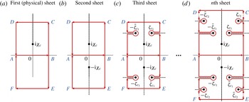
A schematic of integrating contours in different sheets of the Riemann surface in the complex variable
 ${\it\zeta}$
(1.6) near the origin. The first (physical) sheet (a) has a square root singularity only at
 ${\it\zeta}=\text{i}{\it\chi}_{c}$
in
 $\mathbb{C}^{+}.$
Then integrating the ODE (3.4) over the closed contour
 $ABCDA$
provides the analytical continuation into the second sheet (b) of the surface as the branch cut (dashed line) is crossed. As a result,
 $z({\it\zeta})$
does not return to its initial value at the origin
 $0$
. In contrast, integrating the ODE (3.4) over the closed contour
 $ABEFA$
(or over
 $ABCDA$
provided its height falls below
 ${\it\zeta}=\text{i}{\it\chi}_{c}$
), one does not cross the branch cut so
 $z({\it\zeta})$
returns to the same value at the origin with
 $z({\it\zeta})$
remaining in the first sheet. The second sheet has the second square root branch point singularity at
 ${\it\zeta}=-\text{i}{\it\chi}_{c}$
at the lower complex half-plane
 $\mathbb{C}^{-}$
. Integrating over contour
 $ABEFA$
in the second sheet results in the analytical continuation of
 $z({\it\zeta})$
into the third sheet (b) of the Riemann surface. Starting from the third sheet, extra square root branch points appear away from the imaginary axis. Branch cuts for these off-axis singularities are chosen to be extended horizontally as shown by dashed lines in (c,d). The number of these branch points grows with the growth of the sheet number, as schematically shown in (d). We avoid crossing these branch by modifying contours
 $ABCDA$
and
 $ABEFA$
, as shown in (c,d). Note that these two contours must by symmetric with respect to the real line even if the chosen pair of off-axis singularities (symmetric with respect to the imaginary axis) are located only in one of the complex half-planes
 $\mathbb{C}^{+}$
and
 $\mathbb{C}^{-}$
in the given sheet. This is because
 $\bar{z}({\it\zeta})$
is needed for the integration of the ODE (3.4).

Figure 2(a) shows a typical
 $0BCDA0$
rectangular contour for the ODE integration which was used for the analytical continuation of the Stokes wave into the second sheet of Riemann surface. The ODE solution in the second sheet is obtained when the integrating contour crosses the branch cut
 $[\text{i}{\it\chi}_{c},\text{i}]$
. The second subsequent crossing of that branch cut returns
 $z_{ODE}({\it\zeta})$
to the first sheet, confirming the square root branch point at
 ${\it\zeta}=\text{i}{\it\chi}_{c}$
. Figure 3 provides a numerical example of such double crossing. In other words, it was found that the ODE integration along any closed contour in
 ${\it\zeta}\in \mathbb{C}^{+}$
with double crossing of the branch cut (twice integrating along
 $0BCDA0$
) always returns the solution to the original one. If the height of the
 $0BCDA0$
contour is made smaller than
 ${\it\chi}_{c}$
, then there is no crossing of the branch cut and the
 $0BCDA0$
integration returns to the initial value after a single round trip, as shown by dashed curves of figure 3. In a similar way, if the height of
 $0BCDA0$
exceeds 1, then there is no crossing and
 $z_{ODE}({\it\zeta})$
stays in the first sheet (crossing of the branch cut
 $(\text{i},\text{i}\infty )$
corresponds to the jump on
 $2{\rm\pi}$
in the
 $u$
direction in the
 $w$
plane while there is no jump in
 $\tilde{z}$
because of
 $2{\rm\pi}$
-periodicity).
We also verified that there are no singularities in the limit
 $|\text{Re}({\it\zeta})|\rightarrow \infty$
by switching to the ODE integration (3.3) of the
 $w$
variable. In that limit
 $\text{Re}(w)\rightarrow \pm {\rm\pi}$
which allows us to extend the contour in
 $w$
over the entire
 $2{\rm\pi}$
period in the
 $u$
direction (in the
 ${\it\zeta}$
variable it would require us to integrate over the infinite interval
 $-\infty <\text{Re}({\it\zeta})<\infty$
). For all subsequent cases in this section it is assumed that such integration in
 $w$
was performed to check the limit
 $\text{Re}(w)\rightarrow \pm {\rm\pi}$
.
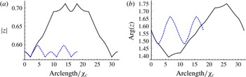
The amplitude
 $|\tilde{z}({\it\zeta})|$
(a) and the argument
 $\text{Arg}(\tilde{z}({\it\zeta}))$
(b) versus arclength in the variable
 ${\it\zeta}$
(scaled by
 ${\it\chi}_{c}$
) along the closed contour
 $0BCDA0$
shown in figure 2(a) (the contour is passed twice in the counterclockwise direction) for ODE integration (which provides the analytical continuation of the Stokes wave in the complex plane) of the Stokes wave solution with
 $H/{\it\lambda}=0.1387112446\ldots$
(corresponding to
 ${\it\chi}_{c}=3.0056373876\ldots \cdot 10^{-3}$
, see table 1 of appendix C for details on the numerical Stokes wave). The contour width is
 $|AB|=2|0B|=2{\it\chi}_{c}$
. Solid lines are for the contour height
 $|BC|=4{\it\chi}_{c}$
(the contour
 $0BCDA0$
twice crosses the branch cut
 $[\text{i}{\it\chi}_{c},\text{i}]$
in the counterclockwise direction) and dotted lines are for the contour height
 $|BC|={\it\chi}_{c}/2$
(for this height, the contour
 $0BCDA0$
does not cross the branch cut
 $[\text{i}{\it\chi}_{c},\text{i}]$
and the total arclength is smaller). It is seen that the solid lines are periodic over the total arclength (two round trips around the contour
 $0BCDA0$
are needed to return to the initial value
 $z(0)$
in the first sheet of the Riemann surface) compared with the half-arclength periodicity of the dotted lines (the contour
 $0BCDA0$
is located in the first sheet only with one roundtrip sufficient to return to the initial value
 $z(0)$
).

The second step of our investigation was to find
 $z({\it\zeta})$
by integrating the ODE (3.4) in the second sheet with
 ${\it\zeta}\in \mathbb{C}^{-}$
using the complex conjugate of
 $z_{ODE}({\it\zeta}),{\it\zeta}\in \mathbb{C}^{+}$
found at previous step to approximate
 $\bar{z}$
and
 $\bar{z}_{{\it\zeta}}$
. The initial condition at that step was at the real line
 ${\it\zeta}=\text{Re}({\it\zeta})$
with
 $z({\it\zeta})$
obtained at the step one for the second sheet.
The second step reveals a new square root singularity at
 ${\it\zeta}=-\text{i}{\it\chi}_{c}$
in the second sheet. Similar to step one, double integration over the contour
 $ABEFA$
shows that
 $z({\it\zeta})$
returns to its original value, confirming that
 ${\it\zeta}=-\text{i}{\it\chi}_{c}$
is the square root branch point. Crossing of the branch cut
 $[-\text{i}{\it\chi}_{c},-\text{i}]$
(corresponding to the new branch point
 ${\it\zeta}=-\text{i}{\it\chi}_{c}$
) allows us to go into the third sheet of the Riemann surface. At that crossing, one has to simultaneously cross from the first to the second sheet for
 $\bar{z}$
and
 $\bar{z}_{{\it\zeta}}$
which again are the complex conjugate of
 $z_{ODE}({\it\zeta}),{\it\zeta}\in \mathbb{C}^{+}$
found at previous step. It was found that the third sheet has branch points both at
 ${\it\zeta}=\text{i}{\it\chi}_{c}$
and
 ${\it\zeta}=-\text{i}{\it\chi}_{c}$
. In a similar way to previous steps, at step three one crosses the branch cut
 $[\text{i}{\it\chi}_{c},\text{i}]$
to go into the fourth sheet of the Riemann surface which is found to have branch points both at
 ${\it\zeta}=\text{i}{\it\chi}_{c}$
and
 ${\it\zeta}=-\text{i}{\it\chi}_{c}$
. At step four, one crosses the branch cut
 $[-\text{i}{\it\chi}_{c},-\text{i}]$
to go into the firth sheet of the Riemann surface which again has branch points both at
 ${\it\zeta}=\text{i}{\it\chi}_{c}$
and
 ${\it\zeta}=-\text{i}{\it\chi}_{c}$
etc. At each sheet,
 $\bar{z},\bar{z}_{{\it\zeta}}$
used in integration of the ODE (3.4) is behind by one in sheet number compared to the current sheet, i.e. values of
 $\bar{z},\bar{z}_{{\it\zeta}}$
from the first, second, third etc. sheets are used for the ODE integration in the second, third, fourth etc. sheets, respectively. After exploring several hundreds of sheets for different values of
 ${\it\chi}_{c}$
, one concludes that the number of sheets is infinite. The double integration over the contours
 $ABCDA$
and
 $ABEFA$
shows that
 ${\it\zeta}=\text{i}{\it\chi}_{c}$
and
 ${\it\zeta}=-\text{i}{\it\chi}_{c}$
are square root branch points in all sheets. In the next section, this conjecture is strengthened by the analysis of expansions at
 ${\it\zeta}=\pm \text{i}{\it\chi}_{c}$
of these multiple sheets.
Starting from the third sheet, extra square root branch points appear away from the imaginary axis. The existence of these off-axis singularities are closely related to the analysis of § 8. They are located significantly further away from the origin than the on-axis
 ${\it\zeta}=\pm \text{i}{\it\chi}_{c}$
singularities. These singularities appear at each sheet, starting from the third one, in pairs located symmetrically with respect to the imaginary axis, as schematically shown in figure 2. The symmetric location of the pairs of singularities is required from the symmetry condition
 $$\begin{eqnarray}\displaystyle \bar{z}(-{\it\zeta})=-z({\it\zeta}). & & \displaystyle\end{eqnarray}$$
That symmetry condition results from the symmetry
 $y(x)=y(-x)$
of the Stokes wave in physical variables. The location of the first pair of off-axis square root singularities at
 ${\it\zeta}=\bar{{\it\zeta}}_{c_{1}}$
and
 ${\it\zeta}=-{\it\zeta}_{c_{1}}$
is schematically shown in figure 2(c). By adaptively increasing the horizontal and vertical sizes of the contour
 $ABEFA$
of figure 2, we found that for
 ${\it\chi}_{c}\ll 1$
the first pair of off-axis square root singularities are located in the third sheet at
 ${\it\zeta}=\bar{{\it\zeta}}_{c_{1}}$
and
 ${\it\zeta}=-{\it\zeta}_{c_{1}}$
with
 $$\begin{eqnarray}\displaystyle \bar{{\it\zeta}}_{c_{1}}\simeq (17.1719-\text{i}10.7734){\it\chi}_{c}. & & \displaystyle\end{eqnarray}$$
Other off-axis pairs are located even further away both from the real and imaginary axes as schematically shown in figure 2. Branch cuts for all off-axis singularities are chosen to be extended horizontally, as shown by the dashed lines in figure 2(c,d). For
 $|A0|,|0B|\lesssim 17.1719{\it\chi}_{c}$
, one can use the same contour as in (a) for all sheets. However, for larger values of
 $|A0|,|0B|$
one has to bypass off-diagonal singularities, as shown in figure 2(c,d), to keep the enumeration of the sheets as described above (based on the on-axis
 ${\it\zeta}=\pm \text{i}{\it\chi}_{c}$
singularities). The number of off-axis branch points grows with an increase of the sheet number. We also performed double integration over closed contours around multiple off-axis singularities and found that each of them is a square root branch point.
A by-product of the ODE integration of this section is that one can also calculate the jump
 $-2{\rm\pi}{\it\rho}({\it\chi})$
(see (2.18)) at the branch cut of the first sheet with high precision. For example, one can start the ODE integration at
 ${\it\zeta}=0$
in the first sheet and integrate until reaching a small neighbourhood of
 ${\it\zeta}=\text{i}{\it\chi}_{c}$
without crossing the branch cut
 ${\it\zeta}\in [\text{i}{\it\chi}_{c},\text{i}]$
. After this, one can integrate the ODE independently along two line segments
 ${\it\zeta}=[\pm {\it\epsilon}+\text{i}{\it\chi}_{c},\pm {\it\epsilon}+\text{i}]$
,
 ${\it\epsilon}\rightarrow 0$
and calculate the difference between these two integrations recovering
 ${\it\rho}({\it\chi})$
with the precision of our simulations,
 ${\sim}10^{-26}$
. A comparison of this high precision
 ${\it\rho}({\it\chi})$
with the numerical approximation of
 ${\it\rho}({\it\chi})$
obtained in Part I from the continuous limit of the Padé approximation (see figures 6b, 7 and 8 in Part I) confirmed the numerical error order estimates of § 6.2 of Part I. Also we found that (4.6)–(4.10) are also in the excellent agreement with the numerical values of
 ${\it\rho}({\it\chi})$
, confirming the asymptotical analysis of § 4.
An ODE of the type (3.4) was numerically integrated in Tanveer (Reference Tanveer1991) based on the Taylor series representation of a Stokes wave in the physical sheet (the additional conformal mapping from the unit disk used in Tanveer (Reference Tanveer1991) onto the half-plane
 $\mathbb{C}^{-}$
of
 ${\it\zeta}$
(1.6) makes that Taylor series similar to the Fourier series representation of Part I (Dyachenko et al.
Reference Dyachenko, Lushnikov and Korotkevich2016)). This representation allowed Tanveer (Reference Tanveer1991) for the first time to extend the numerical integration into the upper half
 $\mathbb{C}^{+}$
of the second Riemann sheet and demonstrate the existence of the square root branch point there. Thus the numerical ODE integration of Tanveer (Reference Tanveer1991) is similar to our first step of this section restricted to
 $\mathbb{C}^{+}$
only.
Note that it was assumed throughout this section that any crossing by the ODE integration contour of both
 $[\text{i},\text{i}\infty ]$
and
 $[-\text{i}\infty ,-\text{i}]$
is avoided. Such a crossing would be harmless in the first sheet because of
 $2{\rm\pi}$
-periodicity of
 $\tilde{z}(w)$
. However, starting from the second sheet,
 $\tilde{z}(w)$
is generally non-periodic in
 $w$
. Thus the branch cuts
 $[\text{i},\text{i}\infty ]$
and
 $[-\text{i}\infty ,-\text{i}]$
can no longer be ignored, contrary to the case of the first sheet discussed in the Introduction. This implies that a crossing of these branch cut provides the additional sheets of the Riemann surface. We however do not explore these sheets here because they have a distance
 $1$
from the real axis in the
 ${\it\zeta}$
plane for any value of
 ${\it\chi}_{c}$
, thus not contributing to the formation of the limiting Stokes wave.
6 Series expansions at
${\it\zeta}=\pm \text{i}{\it\chi}_{c}$
and structure of the Riemann surface for a Stokes wave

Equation (3.1), together with the definition (2.17), show that singularities at
 ${\it\zeta}=\pm \text{i}{\it\chi}_{c}$
are coupled through complex conjugation. We found in Part I (Dyachenko et al.
Reference Dyachenko, Lushnikov and Korotkevich2016) that there is only one singularity (a square root branch point) in the first (physical) sheet of the Riemann surface which corresponds to the finite complex
 $w$
plane. In addition, there is a singularity at
 ${\it\zeta}=\text{i}$
which is the complex infinity
 $w=\text{i}\infty$
and is discussed in § 4. Following Part I, we chose the line segment
 $[\text{i}{\it\chi}_{c},\text{i}]$
as the branch cut connecting these two singularities in the first sheet of the Riemann surface, as sketched on figure 1(a). The singularity at
 ${\it\zeta}=-\text{i}{\it\chi}_{c}$
is not allowed in the first sheet because
 $z$
is analytic in the fluid domain
 $w\in \mathbb{C}^{-}$
.
Consider the expansions in the
 $l$
th sheet of the Riemann surface
 $$\begin{eqnarray}\displaystyle z_{l,+}({\it\zeta})=\mathop{\sum }_{j=0}^{\infty }\text{i}\text{e}^{\text{i}j{\rm\pi}/4}a_{+,l,j}({\it\zeta}-\text{i}{\it\chi}_{c})^{j/2},\quad l=1,2,\ldots , & & \displaystyle\end{eqnarray}$$
and
 $$\begin{eqnarray}\displaystyle z_{l,-}({\it\zeta})=\mathop{\sum }_{j=0}^{\infty }\text{i}\text{e}^{-\text{i}j{\rm\pi}/4}a_{-,l,j}({\it\zeta}+\text{i}{\it\chi}_{c})^{j/2},\quad l=1,2,\ldots , & & \displaystyle\end{eqnarray}$$
where subscripts ‘
 $+$
’ and ‘
 $-$
’ mean expansions at
 ${\it\zeta}=\text{i}{\it\chi}_{c}$
and
 ${\it\zeta}=-\text{i}{\it\chi}_{c}$
, respectively. Here, the branch cuts of
 $({\it\zeta}-\text{i}{\it\chi}_{c})^{1/2}$
and
 $({\it\zeta}+\text{i}{\it\chi}_{c})^{1/2}$
are assumed to extend from
 ${\it\zeta}=\text{i}{\it\chi}_{c}$
upwards and from
 ${\it\zeta}=-\text{i}{\it\chi}_{c}$
downwards, respectively, as shown in figure 1. Often, the location of the branch cut of square root is taken on the negative real axis of the argument. To use this standard agreement about the location of the branch cut, one can replace
 $({\it\zeta}-\text{i}{\it\chi}_{c})^{j/2}$
and
 $({\it\zeta}+\text{i}{\it\chi}_{c})^{j/2}$
in (6.1) and (6.2) by
 $(-\text{i})^{j/2}(\text{i}{\it\zeta}+{\it\chi}_{c})^{j/2}$
and
 $\text{i}^{j/2}(-\text{i}{\it\zeta}+{\it\chi}_{c})^{j/2}$
, respectively.
Following § 5, we enumerate sheets of the Riemann surface according to the branch points
 ${\it\zeta}=\pm \text{i}{\it\chi}_{c}$
as follows. A crossing of the branch cut
 $[\text{i}{\it\chi}_{c},\text{i}]$
in the counterclockwise direction means going from the
 $l=2n-1$
th sheet of the Riemann surface to the
 $l=2n$
th sheet with
 $n=1,2,\ldots \,$
. Case
 $l=1$
corresponds to the physical sheet of the Riemann surface. Similarly, crossing of a branch cut
 $[-\text{i}{\it\chi}_{c},-\text{i}]$
in the counterclockwise direction means going from the
 $l=2n$
th sheet of the Riemann surface to the
 $l=2n+1$
sheet with
 $n=1,2,\ldots$
. Plugging expansions (6.1) and (6.2) into (3.1) and collecting terms of the same order of
 $({\it\zeta}\pm \text{i}{\it\chi}_{c})^{j/2}$
results in the following relations
 $$\begin{eqnarray}\displaystyle \left.\begin{array}{@{}rcl@{}}a_{-,2n,1}\; & =\; & 0,\\ a_{-,2n,2}\; & =\; & \displaystyle \frac{-2}{1-{\it\chi}_{c}^{2}},\\ a_{-,2n,3}\; & =\; & \displaystyle \frac{16c^{2}}{3(1-{\it\chi}_{c}^{2})^{2}a_{+,2n-1,1}(c^{2}-a_{+,2n-1,0}-a_{-,2n,0})},\\ a_{-,2n,4}\; & =\; & \displaystyle \frac{2{\it\chi}_{c}}{(1-{\it\chi}_{c}^{2})^{2}}+\frac{4c^{2}}{(1-{\it\chi}_{c}^{2})^{2}(c^{2}-a_{+,2n-1,0}-a_{-,2n,0})^{2}}\\ \; & \; & -\,\displaystyle \frac{8c^{2}[2+(-1+{\it\chi}_{c}^{2})a_{+,2n-1,2}]}{(1-{\it\chi}_{c}^{2})^{3}a_{+,2n-1,1}^{2}(c^{2}-a_{+,2n-1,0}-a_{-,2n,0})},\\ \; & \; & \hspace{-38.39996pt}\ldots \end{array}\right\} & & \displaystyle\end{eqnarray}$$
for
 $n\geqslant 1$
and
 $$\begin{eqnarray}\displaystyle \left.\begin{array}{@{}rcl@{}}a_{+,2n+1,1}\; & =\; & -\displaystyle \frac{16c^{2}}{3(1-{{\it\chi}_{c}}^{2})^{2}a_{-,2n,3}(c^{2}-a_{-,2n,0}+a_{+,2n+1,0})},\\ a_{+,2n+1,2}\; & =\; & \displaystyle \frac{2}{1-{\it\chi}_{c}^{2}}+\frac{128c^{4}}{9(1-{\it\chi}_{c}^{2})^{4}a_{-,2n,3}^{2}(c^{2}-a_{-,2n,0}-a_{+,2n+1,0})^{3}}\\ \; & \; & +\,\displaystyle \frac{32c^{2}[-2{\it\chi}_{c}+(1-{\it\chi}_{c}^{2})^{2}a_{-,2n,4}]}{9(1-{\it\chi}_{c}^{2})^{4}a_{-,2n,3}^{2}(c^{2}-a_{-,2n,0}-a_{+,2n+1,0})},\\ a_{+,2n+1,3}\; & =\; & \ldots ,\\ \; & \; & \hspace{-46.79993pt}\ldots \end{array}\right\} & & \displaystyle\end{eqnarray}$$
for
 $n\geqslant 1$
.
One cannot take
 $n=0$
in (6.4), which corresponds to
 $l=1$
(the physical sheet of the Riemann surface). This special case has to be considered separately because in the physical sheet, there is no singularity at
 ${\it\zeta}=-\text{i}{\it\chi}_{c}$
(no singularity inside the fluid domain). This implies that
 $$\begin{eqnarray}\displaystyle a_{-,1,2j+1}=0\quad \text{for }j=0,1,2,\ldots & & \displaystyle\end{eqnarray}$$
Solving (6.1), (6.2) and (3.1) for
 $l=1$
with the series expansion at
 ${\it\zeta}=-\text{i}{\it\chi}_{c}$
subject to the condition (6.5) results in the following expressions
 $$\begin{eqnarray}\displaystyle \left.\begin{array}{@{}rcl@{}}a_{+,1,0}\; & =\; & c^{2}-a_{-,1,0},\\ a_{+,1,1}\; & =\; & \displaystyle \frac{-2^{3/2}c}{(1-{\it\chi}_{c}^{2})^{1/2}[2+(1-{\it\chi}_{c}^{2})a_{-,1,2}]^{1/2}},\\ a_{+,1,2}\; & =\; & \displaystyle \frac{4}{3(1-{\it\chi}_{c}^{2})}-\frac{a_{-,1,2}}{3},\\ a_{+,1,3}\; & =\; & -\displaystyle \frac{[(2+(1-{\it\chi}_{c}^{2})a_{-,1,2})]^{5/2}}{2^{1/2}18c(1-{\it\chi}_{c}^{2})^{3/2}}\\ \; & \; & +\,\displaystyle \frac{2^{1/2}c[2{\it\chi}_{c}-2{\it\chi}_{c}(-1+{\it\chi}_{c}^{2})a_{-,1,2}+(-1+{\it\chi}_{c}^{2})^{2}a_{-,1,4}]}{(1-{\it\chi}_{c}^{2})^{3/2}[2+(1-{\it\chi}_{c}^{2})a_{-,1,2}]^{3/2}},\\ a_{+,1,4}\; & =\; & \ldots ,\\ \; & \; & \hspace{-36.0pt}\ldots \end{array}\right\} & & \displaystyle\end{eqnarray}$$
Expressions (6.6) are uniquely determined by values of
 $c$
,
 ${\it\chi}_{c}$
and
 $a_{-,1,2j}$
,
 $j=0,1,2,\ldots$
, where all expressions under square roots are positive and the principle branch of all square roots is assumed. In contrast, the expressions (6.3) and (6.4) are not the unique solutions of (6.1), (6.2) and (3.1). In addition to the solution (6.3), one can obtain two more spurious solutions for
 $a_{-,2n,j}$
. However, these spurious solutions do not correspond to a Stokes wave. One spurious solution has
 $a_{-,2n,2j+1}=0$
for
 $j=1,2,\ldots$
, i.e. it does not have a singularity at
 ${\it\zeta}=-\text{i}{\it\chi}_{c}$
. The second spurious solution has either a radius of convergence well below
 ${\it\chi}_{c}$
or even a zero radius of convergence. Both solutions are spurious because they cannot have the same value in the region of overlap of the disks of convergence of both expansions (6.1) and (6.2). After spurious solutions for
 $a_{-,2n,j}$
are discarded, one obtains the unique solution (6.3) as well as the solution (6.4)
 $a_{+,2n+1,j}$
which also turn out to be uniquely defined. Another peculiar property of the solution (6.3) is that
 $a_{-,2n,1}=0$
while
 $a_{+,2n+1,1}\neq 0$
as given by the solution (6.4).
The right-hand side of (6.4) provides the explicit expressions for the coefficients
 $a_{+,2n+1,j}$
,
 $j=1,2,\ldots$
, for the
 $2n+1$
th sheet of the Riemann surface through the coefficients
 $a_{-,2n,j_{1}}$
,
 $0\leqslant j_{1}\leqslant j+2$
at the
 $2n$
th sheet. The only coefficient which remains unknown is the zeroth coefficient
 $a_{+,2n+1,0}$
for each
 $n\geqslant 1$
. In a similar way, the right-hand side of (6.3) provides the explicit expressions for the coefficients
 $a_{-,2n,j}$
 $j=1,2,\ldots$
, for the
 $2n$
th sheet of the Riemann surface through the coefficients
 $a_{+,2n-1,j_{1}}$
,
 $0\leqslant j_{1}\leqslant j-2$
,
 $j=1,2,\ldots$
, at the
 $2n-1$
th sheet. The only coefficient which remains unknown is the zeroth coefficient
 $a_{-,2n,0}$
for each
 $n\geqslant 1$
.
The explicit expressions for
 $a_{+,2n+1,j}$
and
 $a_{-,2n,j}$
become cumbersome with an increase of
 $j$
beyond the values shown explicitly in (6.3) and (6.4). The explicit expressions
 $a_{+,2n+1,j}$
and
 $a_{-,2n,j}$
were obtained with the help of symbolic computations in the Mathematica 10.2 software. These expressions were used to calculate values of all coefficients
 $a_{+,2n+1,j}$
and
 $a_{-,2n,j}$
for
 $j\geqslant 1$
numerically, with any desired precision (typically we used quadruple (quad) precision with 32 digits accuracy and took into account all
 $j$
in the range
 $1\leqslant j\leqslant 200$
). The remaining coefficients
 $a_{-,2n,0}$
and
 $a_{+,2n+1,0}$
for each
 $n\geqslant 1$
, as well as the numerical value of
 ${\it\chi}_{c}$
, were determined by a numerical procedure which is described below in §§ 6.1 and 6.2.
Values of
 $a_{+,2n+2,j}$
and
 $a_{-,2n+1,j}$
are obtained from
 $a_{+,2n+1,j}$
and
 $a_{-,2n,j}$
by the following relations
 $$\begin{eqnarray}\displaystyle \left.\begin{array}{@{}c@{}}\displaystyle a_{+,2n+2,j}=(-1)^{j}a_{+,2n+1,j},\quad n=0,1,2,\ldots ,\\ \displaystyle a_{-,2n+1,j}=(-1)^{j}a_{-,2n,j},\quad n=1,2,\ldots ,\end{array}\right\} & & \displaystyle\end{eqnarray}$$
which immediately follows from the condition at the crossing of branch cuts.
6.1 Finding of
${\it\chi}_{c}$
, from matching the series expansions at
${\it\zeta}=\pm \text{i}{\it\chi}_{c}$
in the first sheet


Equations (6.6) determine the values of
 $a_{+,1,j}$
,
 $j=0,1,2,\ldots$
from
 $a_{-,1,2j}$
,
 $j=0,1,2,\ldots$
, thus relating the series expansions at
 ${\it\zeta}=-\text{i}{\it\chi}_{c}$
and
 ${\it\zeta}=\text{i}{\it\chi}_{c}$
at the first sheet. The series at
 ${\it\zeta}=-\text{i}{\it\chi}_{c}$
is given by (6.2) with
 $l=1$
together with the condition (6.5). That series contains only integer powers of
 ${\it\zeta}+\text{i}{\it\chi}_{c}$
. The disk of convergence
 $|{\it\zeta}+\text{i}{\it\chi}_{c}|<r$
of that series is determined by the branch point at
 ${\it\zeta}=\text{i}{\it\chi}_{c}$
, which implies that the radius of convergence is
 $r=2{\it\chi}_{c}$
. The series at
 ${\it\zeta}=\text{i}{\it\chi}_{c}$
at the first sheet is given by (6.1), (6.6) and contains both integer and half-integer powers of
 ${\it\zeta}-\text{i}{\it\chi}_{c}$
. The disk of convergence
 $|{\it\zeta}-\text{i}{\it\chi}_{c}|<r$
is determined by the branch point at
 ${\it\zeta}=-\text{i}{\it\chi}_{c}$
of the second sheet. Thus the radius of convergence is also
 $r=2{\it\chi}_{c}$
. In other words, the radius of convergence of the series (6.1), (6.6) in the physical sheet is determined by the singularity in the second (non-physical) sheet.
Numerical values of the coefficients
 $a_{-,1,2j}$
,
 $j=0,1,2,\ldots$
are immediately obtained by the differentiation of the Padé approximants of Part I for each numerical value of
 $H/{\it\lambda}$
. The accuracy of that approximation for the coefficients
 $a_{-,1,2j}$
is checked by plugging these numerical values into the series (6.2) with
 $l=1$
and using (6.5). For numerical evaluation this series is truncated into a finite sum
 $$\begin{eqnarray}\displaystyle z_{1,-,sum}({\it\zeta})=\mathop{\sum }_{j=0}^{j_{max}}\text{i}\text{e}^{-\text{i}j{\rm\pi}/4}a_{-,1,j}({\it\zeta}+\text{i}{\it\chi}_{c})^{j/2}=\mathop{\sum }_{j=0}^{j_{max}/2}\text{i}\text{e}^{-\text{i}j{\rm\pi}/2}a_{-,1,2j}({\it\zeta}+\text{i}{\it\chi}_{c})^{j}, & & \displaystyle\end{eqnarray}$$
where
 $j_{max}$
is chosen sufficiently large to match the numerical precision of the Padé approximants. It is convenient to evaluate this sum at
 ${\it\zeta}=0$
, which is well inside the disk of convergence
 $|{\it\zeta}+\text{i}{\it\chi}_{c}|<2{\it\chi}_{c}$
. It was found that
 $j_{max}=200$
at
 ${\it\zeta}=0$
is sufficient to reach a numerical quad precision of
 ${\sim}10^{-32}$
for the simulations of Part I. This numerical value of
 $j_{max}$
(sufficient to reach quad precision) is only weakly dependent on
 $H/{\it\lambda}$
. To understand this weak dependence, one can note that
 $|{\it\zeta}+\text{i}{\it\chi}_{c}|_{{\it\zeta}=0}={\it\chi}_{c}$
, which is one-half of the radius of convergence of the series (6.2). The asymptotics of the terms of the series (6.2) for large
 $j$
are determined by the radius of convergence as follows
 $|a_{-,1,2j}/a_{-,1,2j+2}|\simeq 2{\it\chi}_{c}.$
Then the truncation of the series (6.2) by the finite sum (6.8) with
 $j_{max}=200$
gives an error
 ${\sim}a_{-,1,j_{max}}{\it\chi}_{c}^{j_{max}/2}\sim 2^{-j_{max}/2}\sim 10^{-30}$
in comparison with the Padé approximation of a Stokes wave at
 ${\it\zeta}=0$
.
It worth noting here that the number of derivatives
 $j_{max}/2=100$
which were reliably recovered above from the Padé approximation was very large, which demonstrates the superior efficiency of the Padé approximation compared with the Fourier series. For example, if instead of the Padé approximation of the Stokes wave one uses the Fourier series representation of the Stokes wave, then the number of derivatives calculated from that series with a high numerical precision would be limited to just a few (approximately 10–20 derivatives if a relative error of
 ${\sim}1$
in the derivatives is allowed).
To obtain numerical values of
 $a_{+,1,j}$
,
 $j=0,1,2,\ldots$
from (6.6) one also has to know the numerical value of
 ${\it\chi}_{c}$
. Part I described a numerical procedure to recover
 ${\it\chi}_{c}$
with an accuracy of
 ${\sim}10^{-10}$
, which is significantly below the accuracy
 ${\lesssim}10^{-26}$
of the numerical Stokes solution itself and its Padé approximation. In this paper, to greatly improve the precision of
 ${\it\chi}_{c}$
, one sets a condition that
 ${\it\chi}_{c}$
is chosen in such a way as to allow the series (6.1) to recover the value of
 $z(0)$
with an accuracy better than
 ${\sim}10^{-26}$
.
Similar to (6.8), the series (6.1) is truncated to a finite sum
 $$\begin{eqnarray}\displaystyle z_{1,+,sum}({\it\zeta})=\mathop{\sum }_{j=0}^{j_{max}}\text{i}\text{e}^{\text{i}j{\rm\pi}/4}a_{+,1,j}({\it\zeta}-\text{i}{\it\chi}_{c})^{j/2},\quad & & \displaystyle\end{eqnarray}$$
where we again choose that
 $j_{max}=200$
, which is enough to match the quad precision of
 ${\sim}10^{-32}$
. Contrary to (6.8), the sum (6.9) includes also half-integer powers of
 ${\it\zeta}-\text{i}{\it\chi}_{c}$
because
 ${\it\zeta}=\text{i}{\it\chi}_{c}$
is the square root branch point. Using (6.6) and (6.9) with the numerical values of
 $a_{-,1,2j}$
,
 $j=0,1,2,\ldots$
, obtained as described in the beginning of this section, one finds in the first sheet a numerical value of
 $z_{1,+,sum}(0)$
for each numerical value of
 ${\it\chi}_{c}$
. Then, numerical Newton (secant) iterations are performed over
 ${\it\chi}_{c}$
aiming to ensure that
 $z_{1,+,sum}(0)$
converges to
 $\simeq z_{pade}(0)$
, i.e.
 ${\it\chi}_{c}$
is chosen such that
 $z_{1,+,sum}(0)$
recovers the value of
 $z_{pade}(0)$
. This provides
 ${\it\chi}_{c}$
with a precision of at least
 $10^{-26}$
, which is limited by the precision of the Padé approximation. Part I also demonstrated the calculation of a Stokes wave well beyond quad precision by using variable precision arithmetics with an achieved accuracy
 ${\sim}200$
digits, thus increasing the accuracy for
 ${\it\chi}_{c}$
is also possible if needed. Table 1 of appendix C provides numerical values of
 ${\it\chi}_{c}$
which correspond to the Padé approximations of the Stokes wave found in Part I.
6.2 Finding
$a_{+,2n+1,0}$
and
$a_{-,2n,0}$
from matching the series expansions at
${\it\zeta}=\pm \text{i}{\it\chi}_{c}$
in the second, third etc. sheets


The procedure for finding numerical values of
 ${\it\chi}_{c}$
and
 $a_{+,1,j}$
,
 $j=0,1,2,\ldots$
described in § 6.1, together with (6.3) and (6.7), allows us to immediately find
 $a_{-,2,j}$
,
 $j=1,2,\ldots$
for each given value of
 $a_{-,2,0}$
. Similar to (6.8) and (6.9), a notation is used such that
 $z_{l,+,sum}({\it\zeta})$
and
 $z_{l,-,sum}({\it\zeta})$
are the finite sums corresponding to the truncation of the series
 $z_{l,+}({\it\zeta})$
(6.1) and
 $z_{l,-}({\it\zeta})$
(6.2), respectively. We assume that
 $j_{max}\simeq 200$
for these finite sums in the sheets
 $l=1,2,\ldots$
. The numerical Newton iterations at the first step are performed over
 $a_{-,2,0}$
, aiming to ensure that
 $z_{2,-,sum}(0)$
converges to
 $z_{2,+,sum}(0)$
. At the second step, the Newton iterations allow us to find
 $a_{+,3,0}$
by matching
 $z_{3,-,sum}(0)$
and
 $z_{3,-,sum}(0).$
In a similar way, the third, fourth etc. steps allow to find
 $a_{-,4,0}$
,
 $a_{+,5,0}$
,
 $a_{-,6,0}$
,
 $a_{+,7,0},\ldots$
Then, using (6.7), one obtains values of
 $a_{+,n,0}$
and
 $a_{-,n,0}$
for all positive integers
 $n$
, completing the analytical continuation of the Stokes wave into the disks
 $|{\it\zeta}\pm \text{i}{\it\chi}_{c}|<2{\it\chi}_{c}$
in the infinite number of sheets of the Riemann surface.
The result of this analytical continuation was compared with the analytical continuation by ODE integration of § 5, giving excellent agreement, which is only limited by the standard numerical accuracy
 ${\sim}10^{-26}$
of the Stokes wave in the physical sheet. Increasing the accuracy of the analytical continuation is straightforward by increasing
 $j_{max}$
for the finite sums
 $z_{l,+,sum}({\it\zeta})$
and
 $z_{l,-,sum}({\it\zeta})$
(and similarly by increasing the accuracy for the ODE integration) provided the Stokes wave precision is increased. Table 3 of appendix C provides a sample of the numerical values of
 $a_{-,2n,0}$
,
 $a_{+,2n+1,0}$
, for
 $n=1,2,3$
obtained by the numerical method outlined in this section.
7 Singularities of the Stokes wave for finite values of
$w$

Grant (Reference Grant1973) and Tanveer (Reference Tanveer1991) showed that the only possible singularity in the finite complex upper half-plane of the physical sheet of the Riemann surface is of a square root type. This result is consistent both with the simulations of Part I (Dyachenko et al. Reference Dyachenko, Lushnikov and Korotkevich2016) and the numerical integration of ODE (3.4) in § 5.
The analysis of Tanveer (Reference Tanveer1991) is based on a version of (3.2) together with the assumption of the analyticity of
 $\bar{z}(w)$
in
 $\mathbb{C}^{+}$
for the first sheet of the Riemann surface. Assume that one performs the ODE integration in the second, third etc. sheets of the Riemann surface as described in §§ 5 and 6, with
 $z(w)$
at the
 $n$
th sheet coupled to
 $\bar{z}(w)$
in the
 $n-1$
th sheet. Here, the counting of sheets follows § 5 and assumes that
 $-{\rm\pi}<\text{Re}(w)<{\rm\pi}$
,
 $|\text{Im}(w)|<\infty$
for all sheets. Then the analysis of Tanveer (Reference Tanveer1991) can be immediately generalized to the
 $n$
th sheet at values of
 $w=w_{1}$
such that
 $z(w)$
has no singularity at
 $w=\bar{w}_{1}$
in the
 $n-1$
th sheet (see (7.16) below). Coupling of the square root singularities at
 ${\it\zeta}=\pm \text{i}{\it\chi}_{c}$
, which is studied in § 6, however goes beyond the analysis of Tanveer (Reference Tanveer1991).
The series expansions of § 6 shows that square root singularities can occur at any finite values of
 $w=w_{1}$
away from the real axis. It was found in § 6 that each square root singularity can either have a counterpart square root singularity at the complex conjugated point
 $w=\bar{w}_{1}$
in the same sheet or can exists without a counterpart singularity at
 $w=\bar{w}_{1}$
, thus going beyond the case analysed by Tanveer (Reference Tanveer1991). A question still remains regarding whether any other type (beyond square root) of coupled singularities at
 $w=w_{1}$
and
 $w=\bar{w}_{1}$
in the same sheet is possible.
Going from the first sheet to the second one, then from the second one to the third one etc., one concludes that the only way for a singularity other than a square root one to appear is if it were coupled with the square root singularity in the previous sheet. Otherwise, it would violate the above mentioned generalization of the result of Tanveer (Reference Tanveer1991) to the arbitrary sheet. Consider a general power-law singularity of
 $z(w)$
at
 $w=w_{1}$
coupled with the square root singularity of
 $\bar{z}(w)$
at
 $w=\bar{w}_{1}$
. We write that general singularity in terms of double series as follows
 $$\begin{eqnarray}\displaystyle z(w)=\mathop{\sum }_{n,m}c_{n,m}(w-w_{1})^{n/2+m{\it\alpha}}, & & \displaystyle\end{eqnarray}$$
where
 ${\it\alpha}$
is a real constant,
 $c_{n,m}$
are complex constants and
 $n,m$
are integers. By shifting
 $n$
and
 $m$
one concludes that without loss of generality one can assume that
 $$\begin{eqnarray}\displaystyle 0<{\it\alpha}<1/2. & & \displaystyle\end{eqnarray}$$
After the complex conjugation, the square root singularity of
 $z(w)$
at
 $w=\bar{w}_{1}$
is given by the following series
 $$\begin{eqnarray}\displaystyle \bar{z}(w)=\mathop{\sum }_{n=0}^{\infty }d_{n}(w-w_{1})^{n/2}, & & \displaystyle\end{eqnarray}$$
where
 $d_{n}$
are complex constants. Coupling of
 $z(w)$
and
 $\bar{z}(w)$
in (3.3) explains why the half-integer powers
 $n/2$
must be taken into account in (7.1). It is convenient to transform from
 $w$
into a new complex variable
 $$\begin{eqnarray}\displaystyle q\equiv (w-w_{1})^{1/2}. & & \displaystyle\end{eqnarray}$$
Equation (3.3) for the new variable
 $q$
takes the following form
 $$\begin{eqnarray}\displaystyle z_{q}=\frac{4q^{2}c^{2}}{\bar{z}_{q}[\text{i}(z-\bar{z})+c^{2}]}. & & \displaystyle\end{eqnarray}$$
The series (7.1) is then transformed into
 $$\begin{eqnarray}\displaystyle z(q)=\mathop{\sum }_{n,m}c_{n,m}q^{n+2m{\it\alpha}}, & & \displaystyle\end{eqnarray}$$
while the series (7.3) runs over integer powers,
 $$\begin{eqnarray}\displaystyle \bar{z}(q)=\mathop{\sum }_{n=0}^{\infty }d_{n}q^{n}. & & \displaystyle\end{eqnarray}$$
The series (7.6) can be also called the
 ${\it\psi}$
-series, see e.g. Hille (Reference Hille1997). If
 ${\it\alpha}$
is a rational number, then in (7.1) one can gather together all terms with the same power of
 $q$
thus reducing (7.1) to a Puiseux series
 $$\begin{eqnarray}\displaystyle z(q)=\mathop{\sum }_{n=-\infty }^{\infty }\tilde{c}_{n}q^{2n/k}, & & \displaystyle\end{eqnarray}$$
where
 $k$
is a positive integer.
If one places the additional restriction that there is no essential singularity at
 $q=0$
, then one has to replace (7.6) with the truncated series
 $$\begin{eqnarray}\displaystyle z(q)=\mathop{\sum }_{n\geqslant n_{0},m\geqslant m_{0}}c_{n,m}q^{n+2m{\it\alpha}}, & & \displaystyle\end{eqnarray}$$
for the integer constants
 $n_{0}$
and
 $m_{0}$
. Plugging (7.7) and (7.9) into the Stokes wave (7.5), moving the denominator to the left-hand side in (7.5) and collecting terms with the same power of
 $q$
, starting from the lowest power, one obtains that
 $2{\it\alpha}$
must be an integer for any values of
 $n_{0}$
and
 $m_{0}$
and all values of
 $d_{n}$
. Thus no new solutions in the form (7.9) exist beyond those was found in § 6.
One can also study the singularities using the classification of movable and fixed singularities in nonlinear ODEs of first order in the general form
 $z_{q}=f(q,z)$
Golubev (Reference Golubev1950), Ince (Reference Ince1956), Hille (Reference Hille1997). The positions of fixed singularities for the independent complex variable
 $q$
are determined by the properties of the ODE, i.e. by singularities of the function
 $f(q,z)$
. In contrast, the position of a movable singularity is not fixed but typically is determined by an arbitrary complex constant. To analyse the singularities, it is convenient to introduce a new unknown
 $$\begin{eqnarray}\displaystyle {\it\xi}(q)\equiv \frac{1}{\text{i}(z-\bar{z})+c^{2}}. & & \displaystyle\end{eqnarray}$$
Then (7.5) takes the following form
 $$\begin{eqnarray}\displaystyle {\it\xi}_{q}=\text{i}\bar{z}_{q}{\it\xi}^{2}-\frac{4\text{i}q^{2}c^{2}{\it\xi}^{3}}{\bar{z}_{q}}, & & \displaystyle\end{eqnarray}$$
where
 $\bar{z}(q)$
is assumed to be known and is determined by
 $z(\bar{q})$
from the previous sheet of the Riemann surface. Equation (7.11) has a cubic polynomial right-hand side in
 ${\it\xi}$
which ensures that it has a movable square root singularity
 $$\begin{eqnarray}\displaystyle {\it\xi}=\mathop{\sum }_{n=-1}^{\infty }c_{n}(q-C)^{n/2}, & & \displaystyle\end{eqnarray}$$
provided
 $C\neq 0$
,
 $\bar{z}_{q}(C)\neq 0$
(see e.g. Golubev Reference Golubev1950; Ince Reference Ince1956; Hille Reference Hille1997), where
 $c_{n}$
and
 $C$
are complex constants. Using (7.4), (7.10) and the condition
 $C\neq 0$
, one recovers the expansion (7.3) with
 $w_{1}$
replaced by
 $w_{1}+C^{2}$
, thus the movable singularity (7.12) is reduced to the square root singularity in
 $w$
.
Equation (7.11) has a fixed singularity at
 $q=0$
provided
 $\bar{z}_{q}(0)\neq 0$
. To show that one uses a new unknown
 ${\it\psi}\equiv 1/{\it\xi}$
to transform (7.11) into
 $$\begin{eqnarray}\displaystyle {\it\psi}_{q}=\frac{-\text{i}\bar{z}_{q}^{2}{\it\psi}+4\text{i}q^{2}c^{2}}{\bar{z}_{q}{\it\psi}}, & & \displaystyle\end{eqnarray}$$
which has
 $0/0$
singularity in right-hand side for
 $q={\it\psi}=0$
, satisfying the criteria for the existence of a fixed singularity (see Golubev Reference Golubev1950; Hille Reference Hille1997).
Consider now a particular case
 $\bar{z}_{q}(0)=0$
and
 $\bar{z}_{qq}(0)\neq 0$
which corresponds to the expansion (6.3). One can define a new function
 $$\begin{eqnarray}\displaystyle g(q)\equiv \frac{\tilde{z}_{q}}{q},\quad g(0)\neq 0 & & \displaystyle\end{eqnarray}$$
and rewrite (7.13) as follows
 $$\begin{eqnarray}\displaystyle {\it\psi}_{q}=\frac{-\text{i}qg(q)^{2}{\it\psi}+4\text{i}qc^{2}}{g(q){\it\psi}}. & & \displaystyle\end{eqnarray}$$
Generally, this equation still has a fixed singularity because of the
 $0/0$
singularity in right-hand side. However, in the particular case when
 $g(q)$
is an even function of
 $q$
, one can define the function
 $\tilde{g}(q^{2})\equiv g(q)$
, which is analytic in the variable
 $\tilde{q}\equiv q^{2}$
at
 $q=0$
. This case means that
 $z(w)$
is analytic at
 $w=w_{1}$
. Then one transforms (7.15) into the equation
 $$\begin{eqnarray}\displaystyle {\it\psi}_{\tilde{q}}=\frac{-\text{i}\tilde{g}(\tilde{q})^{2}{\it\psi}+4\text{i}c^{2}}{2\tilde{g}(\tilde{q}){\it\psi}}, & & \displaystyle\end{eqnarray}$$
which does not have a fixed singularity. Equation (7.16) together with (7.12) reproduce the result of Tanveer (Reference Tanveer1991) applied to all sheets of the Riemann surface.
Thus the approaches reviewed in Golubev (Reference Golubev1950), Ince (Reference Ince1956), Hille (Reference Hille1997) applied to (7.5) are consistent with square root singularities and the series expansions of § 6 for all sheets of the Riemann surface. However, these approaches cannot exclude the possibility of the existence of other types of singularity. Note that examples given in Golubev (Reference Golubev1950), Ince (Reference Ince1956), Hille (Reference Hille1997) also show that the existence of the fixed singularity in the ODE at the point
 $q=0$
does not necessary mean that the singularity occurs in the general ODE solution
 $z(q)$
at that point.
One concludes that a coupling of the essential singularity at
 $w=w_{1}$
with the square root singularity at
 $w=\bar{w}_{1}$
cannot be excluded neither by the series analysis used in (7.4)–(7.9) nor by looking at the fixed ODE singularities through (7.10)–(7.15). However, the simulations of § 5 and series expansions of § 6 clearly indicate the absence of any singularities beyond the square roots ones in all sheets of the Riemann surface for the non-limiting Stokes wave in
 ${\it\zeta}\in \mathbb{C}\diagdown ((-\text{i}\infty ,-\text{i}]\cup ([\text{i},\text{i}\infty )))$
(i.e. everywhere in the complex plane
 $\mathbb{C}$
except the branch cuts
 $(-\text{i}\infty ,-\text{i}]$
and
 $[\text{i},\text{i}\infty )$
). In the first sheet the branch cuts
 $(-\text{i}\infty ,-\text{i}]$
and
 $[\text{i},\text{i}\infty )$
are not significant, as explained in the Introduction, and the only a non-square root singularity exists at
 ${\it\zeta}=\text{i}$
, see § 4. It is conjectured here that non-square root singularities do not appear in all sheets of the Riemann surface for
 ${\it\zeta}\in \mathbb{C}\diagdown ((-\text{i}\infty ,-\text{i}]\cup [\text{i},\text{i}\infty ))$
.
As discussed at the end of § 5, singularities are possible at the boundary of the strip
 $\text{Re}(w)=\pm {\rm\pi}$
which corresponds to the branch cuts
 $[\text{i},\text{i}\infty )$
and
 $[-\text{i}\infty ,-\text{i})$
in the
 ${\it\zeta}$
plane. However, these branch cuts are separated by the distance
 ${\rm\pi}$
from the origin in the
 $w$
plane (or by the distance
 $1$
in the
 ${\it\zeta}$
plane) and they cannot explain the formation of the limiting Stokes wave as
 $v_{c}\rightarrow 0$
. The same is true for the singularity at
 $w\rightarrow \text{i}\infty$
(
 ${\it\zeta}\rightarrow \text{i}$
) analysed in § 4.
8 Conjecture on recovering of the
$2/3$
power law of the limiting Stokes wave from an infinite number of nested square root singularities of a non-limiting Stokes wave as
${\it\chi}_{c}\rightarrow 0$


One concludes from §§ 6 and 7 that the only possibility for the formation of a
 $2/3$
power-law singularity (1.1) of the limiting Stokes wave is through the merging of an infinite number of square root singularities from different sheets of the Riemann surface in the limit
 $v_{c}\rightarrow 0$
. The total number of square root singularities could be either finite or infinite for
 $v_{c}>0$
, both cases are compatible with the expansions of § 6 (although an infinite number of singularities appears to hold for the generic values of the expansion coefficients of § 6). Both numerical ODE integration of § 5 and series expansions of § 6 reveal that the number of sheets of the Riemann surface related to the singularities at
 ${\it\zeta}=\pm \text{i}{\it\chi}_{c}$
exceeds several hundred for a wide range of numerical values
 $10^{-7}\lesssim {\it\chi}_{c}\lesssim 0.2$
. This suggests that the number of sheets is infinite for all values of
 $v_{c}$
. In any case, the number of singularities must be infinite as
 $v_{c}\rightarrow 0$
.
Here, a conjecture is made that the limiting Stokes wave occurs at the limit
 $v_{c}\rightarrow 0$
of the following leading-order solution
 $$\begin{eqnarray}\displaystyle & & \displaystyle z=\text{i}\frac{c^{2}}{2}+c_{1}{\it\chi}_{c}^{1/6}\sqrt{{\it\zeta}-\text{i}{\it\chi}_{c}}\nonumber\\ \displaystyle & & \displaystyle \quad +\,\frac{(3c)^{2/3}}{2}\text{e}^{-\text{i}{\rm\pi}/6}[({\it\zeta}-\text{i}{\it\chi}_{c})^{1/2}+(-2\text{i}{\it\chi}_{c})^{1/2}]\sqrt{{\it\alpha}_{1}{\it\chi}_{c}^{1/4}+\sqrt{({\it\zeta}-\text{i}{\it\chi}_{c})^{1/2}+(-2\text{i}{\it\chi}_{c})^{1/2}}}\nonumber\\ \displaystyle & & \displaystyle \quad \times \,\sqrt{{\it\alpha}_{3}{\it\chi}_{c}^{1/16}+\sqrt{{\it\alpha}_{2}{\it\chi}_{c}^{1/8}+\sqrt{{\it\alpha}_{1}{\it\chi}_{c}^{1/4}+\sqrt{({\it\zeta}-\text{i}{\it\chi}_{c})^{1/2}+(-2\text{i}{\it\chi}_{c})^{1/2}}}}}\nonumber\\ \displaystyle & & \displaystyle \quad \times \,\sqrt{{\it\alpha}_{2n+1}{\it\chi}_{c}^{1/2^{2n+2}}\!+\!\sqrt{{\it\alpha}_{2n}{\it\chi}_{c}^{1/2^{2n+1}}\!+\!\sqrt{\cdots +\sqrt{{\it\alpha}_{1}{\it\chi}_{c}^{1/4}\!+\!\sqrt{({\it\zeta}-\text{i}{\it\chi}_{c})^{1/2}\!+\!(-2\text{i}{\it\chi}_{c})^{1/2}}}}}}\quad \nonumber\\ \displaystyle & & \displaystyle \quad \times \,\cdots +\frac{(3c)^{2/3}}{2}\text{e}^{-\text{i}{\rm\pi}/6}[({\it\zeta}-\text{i}{\it\chi}_{c})^{1/2}+(-2\text{i}{\it\chi}_{c})^{1/2}]\nonumber\\ \displaystyle & & \displaystyle \quad \times \,\sqrt{\tilde{{\it\alpha}}_{1}{\it\chi}_{c}^{1/4}+\sqrt{({\it\zeta}-\text{i}{\it\chi}_{c})^{1/2}+(-2\text{i}{\it\chi}_{c})^{1/2}}}\nonumber\\ \displaystyle & & \displaystyle \quad \times \,\sqrt{\tilde{{\it\alpha}}_{3}{\it\chi}_{c}^{1/16}\!+\!\sqrt{\tilde{{\it\alpha}}_{2}{\it\chi}_{c}^{1/8}\!+\!\sqrt{\tilde{{\it\alpha}}_{1}{\it\chi}_{c}^{1/4}\!+\!\sqrt{({\it\zeta}-\text{i}{\it\chi}_{c})^{1/2}\!+\!(-2\text{i}{\it\chi}_{c})^{1/2}}}}}\nonumber\\ \displaystyle & & \displaystyle \quad \times \,\sqrt{\tilde{{\it\alpha}}_{2n+1}{\it\chi}_{c}^{1/2^{2n+2}}+\sqrt{\tilde{{\it\alpha}}_{2n}{\it\chi}_{c}^{1/2^{2n+1}}+\sqrt{\cdots +\sqrt{\tilde{{\it\alpha}}_{1}{\it\chi}_{c}^{1/4}+\sqrt{({\it\zeta}-\text{i}{\it\chi}_{c})^{1/2}+(-2\text{i}{\it\chi}_{c})^{1/2}}}}}}\nonumber\\ \displaystyle & & \displaystyle \quad \times \cdots +\text{h.o.t.},\end{eqnarray}$$
which is the infinite product of increasingly nested square roots. This conjecture was first presented in Lushnikov, Dyachenko & Korotkevich (Reference Lushnikov, Dyachenko and Korotkevich2015). Equation (8.1) has two terms with nested roots, one with non-zero complex constants
 ${\it\alpha}_{1},{\it\alpha}_{2},{\it\alpha}_{3},{\it\alpha}_{4},\ldots$
and another with non-zero complex constants
 $\tilde{{\it\alpha}}_{1},\tilde{{\it\alpha}}_{2},\tilde{{\it\alpha}}_{3},\tilde{{\it\alpha}}_{4},\ldots$
which are related through complex conjugation as follows
 $$\begin{eqnarray}\displaystyle \tilde{{\it\alpha}}_{1}=\bar{{\it\alpha}}_{1}\text{e}^{-\text{i}{\rm\pi}/4},\quad \tilde{{\it\alpha}}_{2}=\bar{{\it\alpha}}_{1}\text{e}^{-\text{i}{\rm\pi}/8},\ldots ,\tilde{{\it\alpha}}_{n}=\bar{{\it\alpha}}_{n}\text{e}^{-\text{i}{\rm\pi}/2^{n+1}},\ldots & & \displaystyle\end{eqnarray}$$
All these constants, including another complex constant
 $c_{1}$
, are of the order of
 $O(1)$
independent of
 ${\it\chi}_{c}$
. The relations (8.2) ensure that the symmetry condition (5.2) is satisfied.
At
 ${\it\zeta}\gg {\it\chi}_{c}$
one obtains from (8.1), using the asymptotic of products of all square roots, that
 $$\begin{eqnarray}\displaystyle z\propto {\it\zeta}^{1/2+1/8+1/32+1/128+\cdots }={\it\zeta}^{2/3} & & \displaystyle\end{eqnarray}$$
exactly reproducing the Stokes solution (1.1) while the term
 $c_{1}{\it\chi}_{c}^{1/6}\sqrt{{\it\zeta}-\text{i}{\it\chi}_{c}}$
vanishes as
 ${\it\chi}_{c}\rightarrow 0$
. For small but finite
 ${\it\chi}_{c}$
, the limiting Stokes solution (1.1) is valid for
 ${\it\chi}_{c}\ll {\it\zeta}\ll 1$
, as seen from (8.1). For
 ${\it\zeta}\sim 1$
, the higher-order terms denoted by h.o.t. both in (1.1) and (8.1), become important such as the term with the irrational power
 $$\begin{eqnarray}\displaystyle \propto {\it\zeta}^{{\it\mu}},{\it\mu}=1.4693457\ldots & & \displaystyle\end{eqnarray}$$
(Grant Reference Grant1973; Williams Reference Williams1981).
Different branches of all nested square roots in (8.1) choose different sheets of the Riemann surface following the numeration of sheets used in § 5. In particular, the principal branch of
 $({\it\zeta}-\text{i}{\it\chi}_{c})^{1/2}$
in the expression
 $g({\it\zeta})\equiv ({\it\zeta}-\text{i}{\it\chi}_{c})^{1/2}+(-2\text{i}{\it\chi}_{c})^{1/2}$
corresponds to the first sheet. To understand this, one expands
 $g({\it\zeta})$
at
 ${\it\zeta}=-\text{i}{\it\chi}_{c}$
, which results in
 $$\begin{eqnarray}\displaystyle g_{+}({\it\zeta})=2(-2\text{i}{\it\chi}_{c})^{1/2}+\frac{{\it\zeta}+\text{i}{\it\chi}_{c}}{2(-2\text{i}{\it\chi}_{c})^{1/2}}+O({\it\zeta}+\text{i}{\it\chi}_{c})^{2}, & & \displaystyle\end{eqnarray}$$
where the subscript ‘
 $+$
’ means taking the principle branch of
 $({\it\zeta}-\text{i}{\it\chi}_{c})^{1/2}$
. For the second (negative) branch of
 $({\it\zeta}-\text{i}{\it\chi}_{c})^{1/2}$
one obtains that
 $$\begin{eqnarray}\displaystyle g_{-}({\it\zeta})=-\frac{{\it\zeta}+\text{i}{\it\chi}_{c}}{2(-2\text{i}{\it\chi}_{c})^{1/2}}+O({\it\zeta}+\text{i}{\it\chi}_{c})^{2}, & & \displaystyle\end{eqnarray}$$
with the subscript ‘
 $-$
’ meaning that second branch.
The expression
 $g({\it\zeta})$
enters under the most inner square root into each term of the product in (8.1). Then, using the expansion (8.5), one obtains that the series expansion of (8.1) at
 ${\it\zeta}=-\text{i}{\it\chi}_{c}$
contains only non-negative integer powers of
 ${\it\zeta}+\text{i}{\it\chi}_{c}$
, thus confirming that
 $z({\it\zeta})$
is analytic at
 ${\it\zeta}=-\text{i}{\it\chi}_{c}$
. This means that the condition (6.5) is satisfied. In contrast, taking the expansion (8.6) one obtains that the series expansion of (8.1) at
 ${\it\zeta}=-\text{i}{\it\chi}_{c}$
is of the type (6.2) containing non-negative half-integer powers of
 ${\it\zeta}+\text{i}{\it\chi}_{c}$
, as expected for all sheets starting from the second sheet. In addition, the term
 $g({\it\zeta})$
in the square brackets in (8.1) ensures that
 $a_{-,2n,1}=0$
, as required by (6.3). The expansion of (8.1) at
 ${\it\zeta}=\text{i}{\it\chi}_{c}$
has half-integer powers of
 ${\it\zeta}-\text{i}{\it\chi}_{c}$
for both branches of
 $g({\it\zeta})$
, thus being consistent with the square root singularity at
 ${\it\zeta}=\text{i}{\it\chi}_{c}$
in all sheets of the Riemann surface, including the first sheet, in agreement with (6.1), (6.4) and (6.6).
Choosing two possible branches of all other nested square roots (besides the most inner square root) in (8.1) one obtains the expansions (6.1) and (6.2), at
 ${\it\zeta}=\pm \text{i}{\it\chi}_{c}$
with different coefficients
 $a_{+,l,j}$
and
 $a_{-,l,j}$
at each
 $l$
th sheet. The values of these coefficients are determined by the values of
 ${\it\chi}_{c},c_{1},{\it\alpha}_{1},{\it\alpha}_{2},{\it\alpha}_{3},{\it\alpha}_{4},\ldots$
together with the contribution from the h.o.t. terms in (8.1). One concludes that the ansatz (8.1) is consistent with the properties of a non-limiting Stokes wave studied in this paper, which motivates conjecture (8.1). Also, the coefficients
 ${\it\alpha}_{1},{\it\alpha}_{2},{\it\alpha}_{3},\ldots$
determine additional square root branch points which are located away from the imaginary axis at a distance larger than
 ${\it\chi}_{c}$
from the origin in the third and higher sheets of the Riemann surface. Values of these coefficients can be determined from the locations of the branch points independently recovered from the integration, similar to what is described in § 5 (see also § 8.1 for an example of recovering
 ${\it\alpha}_{1}$
).
8.1 Numerical verification of the conjecture
Now we provide a numerical demonstration of the efficiency of the conjecture (8.1) by using the simplest non-trivial approximation of (8.1) which takes into account only the threefold nested roots as follows
 $$\begin{eqnarray}\displaystyle z & \simeq & \displaystyle \left(\text{i}\frac{c^{2}}{2}+c_{0}{\it\chi}_{c}^{2/3}\right)+c_{1}{\it\chi}_{c}^{1/6}\sqrt{{\it\zeta}-\text{i}{\it\chi}_{c}}+c_{2}{\it\zeta}\nonumber\\ \displaystyle & & \displaystyle +\,c_{3}{\it\chi}_{c}^{1/24}[({\it\zeta}-\text{i}{\it\chi}_{c})^{1/2}+(-2\text{i}{\it\chi}_{c})^{1/2}]\sqrt{{\it\alpha}_{1}{\it\chi}_{c}^{1/4}+\sqrt{({\it\zeta}-\text{i}{\it\chi}_{c})^{1/2}+(-2\text{i}{\it\chi}_{c})^{1/2}}}\nonumber\\ \displaystyle & & \displaystyle +\,\bar{c}_{3}\text{e}^{(-3\text{i}{\rm\pi})/8}{\it\chi}_{c}^{1/24}[({\it\zeta}-\text{i}{\it\chi}_{c})^{1/2}+(-2\text{i}{\it\chi}_{c})^{1/2}]\nonumber\\ \displaystyle & & \displaystyle \times \,\sqrt{\bar{{\it\alpha}}_{1}\text{e}^{(-\text{i}{\rm\pi})/4}{\it\chi}_{c}^{1/4}+\sqrt{({\it\zeta}-\text{i}{\it\chi}_{c})^{1/2}+(-2\text{i}{\it\chi}_{c})^{1/2}}},\end{eqnarray}$$
where we have added the term
 $c_{2}{\it\zeta}$
, as well the constants
 $c_{0}$
,
 $c_{2}$
and
 $c_{3}$
, to approximate the neglecting of the other nested roots (which include
 ${\it\alpha}_{2},{\it\alpha}_{3},\ldots$
) in comparison with (8.1). In other words, we approximate all the more than threefold nested roots in (8.1) by Taylor series expansion, keeping only the constant and linear terms in
 ${\it\zeta}$
in that expansion. The constant terms result in adding the constants
 $c_{3}$
and
 $\bar{c}_{3}$
in front of the nested roots as well as in the addition of the small correction
 $c_{0}{\it\chi}_{c}^{2/3}$
to the constant term
 $\text{i}c^{2}/2$
of (8.1). The linear terms result in the appearance of the constant
 $c_{2}$
replacing higher-order nested roots of (8.1). Also, the factor
 $\bar{c}_{3}\text{e}^{(-3\text{i}{\rm\pi})/8}$
ensures the symmetry (5.2) and the additional scaling
 ${\it\chi}_{c}^{1/24}$
provides for
 ${\it\zeta}\sim {\it\chi}_{c}$
the same total scaling
 $\propto {\it\chi}_{c}^{2/3}$
of the nested square roots of (8.7) as in (8.1). The approximation (8.1) can be valid only up to moderately large values of
 $\text{Re}({\it\zeta})={\it\zeta}$
(a comparison with (8.1) suggests that it could be valid up to values of
 ${\it\zeta}$
in several tens of
 ${\it\chi}_{c}$
after which higher-order nested roots must come into play).
To find the numerical values of
 ${\it\alpha}_{1}$
,
 $c_{0}$
,
 $c_{1},c_{2}$
and
 $c_{3}$
without any fit we use the following procedure. At the first step, we determine from the contour integration of § 5 the location (5.3) of the first pair of off-axis square root singularities (located at
 ${\it\zeta}=\bar{{\it\zeta}}_{c_{1}}$
and
 ${\it\zeta}=-{\it\zeta}_{c_{1}}$
). Then we solve equation
 ${\it\alpha}_{1}{\it\chi}_{c}^{1/4}+\sqrt{(\bar{{\it\zeta}}_{c_{1}}-\text{i}{\it\chi}_{c})^{1/2}+(-2\text{i}{\it\chi}_{c})^{1/2}}=0$
. (It corresponds to the zero under the threefold square root in (8.1)) in the third sheet of the Riemann surface. Then, together with (5.3) it gives that
 $$\begin{eqnarray}\displaystyle {\it\alpha}_{1}\simeq -0.0955383-\text{i}1.8351. & & \displaystyle\end{eqnarray}$$
Note that the second square root
 ${\it\zeta}=-{\it\zeta}_{c_{1}}$
(symmetric with respect to the imaginary axis) is ensured by the similar term with
 $\bar{{\it\alpha}}_{1}\text{e}^{(-\text{i}{\rm\pi})/4}$
in (8.7). At the second step, we expand (8.1) in the first sheet of the Riemann surface in powers of
 $({\it\zeta}-\text{i}{\it\chi}_{c})^{1/2}$
. After that, we match the first five coefficients of that expansion to the analytical expressions of the coefficients
 $a_{+,1,j}$
,
 $j=1,\ldots ,5$
, of the expansion (6.6) obtained in § 6. This matching results in explicit expressions for
 $c_{0}$
,
 $c_{1},c_{2}$
and
 $c_{3}$
. For example, for a Stokes wave with
 ${\it\chi}_{c}=2.9691220994\ldots \times 10^{-7}$
(corresponding to the last line of table 1 of appendix C, see that Appendix for more details on the numerical Stokes wave) we obtain that
 $c_{0}=\text{i}17.1920\ldots$
,
 $c_{1}=\text{e}^{-\text{i}{\rm\pi}/4}3.81499\ldots ,c_{2}=-1.8779\ldots$
and
 $c_{3}=1.42696\ldots -\text{i}1.8849\ldots$
. Changing of
 ${\it\chi}_{c}$
by several orders of magnitude results in changing these coefficients only within the range 5 %–10 %.
A comparison of the limiting Stokes wave (dotted line) with (8.7) and the numerical solution for the Stokes wave (the last two of these are shown by the single solid line because they are visually indistinguishable with maximum difference between them
 $\simeq 4\times 10^{-6}$
) for
 ${\it\chi}_{c}=2.9691220994\ldots \times 10^{-7}$
. Solid line corresponds to
 $-50{\it\chi}_{c}\leqslant {\it\zeta}\leqslant 50{\it\chi}_{c}$
.

We demonstrated the efficiency of the obtained numerical values of
 $c_{0}$
,
 $c_{1},c_{2}$
and
 $c_{3}$
in two independent ways. In the first way, it was checked that the coefficients
 $a_{+,1,j}$
of (6.6) for
 $j=6,\ldots$
are well reproduced (within
 $4\,\%$
and
 $7\,\%$
accuracy for
 $j\leqslant 10$
and
 $j\leqslant 100$
, respectively) by the expansion of (8.7) with the same numerical values of
 $c_{0}$
,
 $c_{1},c_{2}$
and
 $c_{3}$
. This implies that the approximate expression (8.7) captures the significant property of the convergence of the series (6.6) rather than being just the match of the few first terms of that series. The second way of efficiency demonstration is provided in figure 4, where excellent agreement is shown between the numerical solution of the Stokes wave from Part I (Dyachenko et al.
Reference Dyachenko, Lushnikov and Korotkevich2016) and the expression (8.7) for
 $-50{\it\chi}_{c}\leqslant {\it\zeta}\leqslant 50{\it\chi}_{c}$
. This range of
 ${\it\zeta}$
is far beyond the disk of convergence
 $|{\it\zeta}-\text{i}{\it\chi}_{c}|<2{\it\chi}_{c}$
of the series (6.6).
9 Concluding remarks
In summary, it was found that the Riemann surface corresponding to a non-limiting Stokes wave consists of an infinite number of sheets corresponding to an infinite number of square root branch points located at
 ${\it\zeta}=\pm \text{i}{\it\chi}_{c}$
in all sheets except the first sheet. The first (physical) sheet has only one singularity at
 ${\it\zeta}=\text{i}{\it\chi}_{c}$
while avoiding a singularity at
 ${\it\zeta}=-\text{i}{\it\chi}_{c}$
which ensures that the Stokes wave represents the analytical solution inside the fluid domain. Two means of analytical continuation into all these sheets were used, the first based on ODE integration of § 5 and the second based on the coupled series expansions (6.1)–(6.6) in half-integer powers at
 ${\it\zeta}=\pm \text{i}{\it\chi}_{c}$
.
To go beyond the disks of convergence
 $|{\it\zeta}\pm \text{i}{\it\chi}_{c}|<2{\it\chi}_{c}$
of the series expansions (6.1)–(6.6), it is conjectured in § 8 that the leading-order form of a non-limiting Stokes wave consists of an infinite number of nested square roots (8.1). These nested square roots can recover the series expansions (6.1)–(6.6) within their disks of convergence
 $|{\it\zeta}\pm \text{i}{\it\chi}_{c}|<2{\it\chi}_{c}$
. For
 $|{\it\zeta}\pm \text{i}{\it\chi}_{c}|\gg {\it\chi}_{c}$
, well beyond these disks of convergence, the asymptotic (8.3) is valid, thus ensuring the nested square roots have the form of the
 $2/3$
power-law singularity of the limiting Stokes wave in the limit
 ${\it\chi}_{c}\rightarrow 0$
.
There are two other infinite sequences of Riemann sheets resulting from (i) off-axis square root singularities in the third and higher sheets of Riemann surface, as analysed in §§ 5 and 8 and (ii) the singularity at
 ${\it\zeta}=\text{i}$
(corresponding to
 $w=\text{i}\infty$
) which involves logarithms, as analysed in § 4. However, these extra sheets do not contribute to the qualitative change of the power-law singularity from
 $1/2$
(non-limiting Stokes wave) to
 $2/3$
(limiting Stokes wave) near the origin, as given by the asymptotic (8.3). However, these extra sheets are expected to be important for the analysis of a Stokes wave for
 ${\it\zeta}\sim 1$
, where the higher-order terms become important, such as the term (8.4) with irrational power (Grant Reference Grant1973; Williams Reference Williams1981). The analysis of these terms is beyond the scope of this paper. These terms might be also essential to answer the question left open by Longuet-Higgins & Fox (Reference Longuet-Higgins and Fox1977), McLeod (Reference McLeod1997) regarding whether the number of oscillations in the slope of a non-limiting Stokes wave increases to infinity as a non-limiting Stokes wave approaches its limiting form. Note that these oscillations vanish for the limiting Stokes wave, as was proven in Plotnikov & Toland (Reference Plotnikov and Toland2004).
Appendix A. Equivalence of two forms of the equation for a Stokes wave
In this Appendix we show that both forms (2.1) and (3.1) of the equation for a Stokes wave are equivalent to each other. Then § 2 implies that (2.13) and (2.22) are also equivalent to (2.1) and (3.1). Equation (2.1) was obtained by Dyachenko et al. (Reference Dyachenko, Kuznetsov, Spector and Zakharov1996) while (3.1) in slightly different forms was used by numerous authors including Grant (Reference Grant1973), Schwartz (Reference Schwartz1974), Longuet-Higgins & Fox (Reference Longuet-Higgins and Fox1977), Stokes (Reference Stokes1880b ), Williams (Reference Williams1981) and Tanveer (Reference Tanveer1991). Appendix B explains the derivation of (3.1) starting from the basic equations of potential flow of an ideal fluid with a free surface.
Applying the Hilbert operator
 ${\hat{H}}$
(2.2) to (2.1) and using the relations (2.14) and (2.15) one obtains that
 $$\begin{eqnarray}\displaystyle c^{2}\tilde{x}_{u}-yx_{u}+{\hat{H}}[yy_{u}]=0, & & \displaystyle\end{eqnarray}$$
which is equivalent to (2.13). We define a new variable
 $$\begin{eqnarray}\displaystyle f\equiv -{\hat{H}}[yy_{u}] & & \displaystyle\end{eqnarray}$$
and split it into two functions
 $$\begin{eqnarray}\displaystyle f=f^{+}+f^{-}, & & \displaystyle\end{eqnarray}$$
using (2.4), (2.7), (2.8) and (2.9) such that
 $f^{+}$
and
 $f^{-}$
are the functions which are analytic in upper half-plane
 $\mathbb{C}^{+}$
and lower complex half-plane
 $\mathbb{C}^{-}$
of
 $w$
, respectively. Note that the zeroth harmonic
 $f_{0}=0$
as follows from the definition (A 2). Taking the linear combination of
 $f$
and
 ${\hat{H}}f$
, using (2.1), (A 1) and (A 2), one finds that
 $$\begin{eqnarray}\displaystyle x_{u}{\hat{H}}f+y_{u}f=c^{2}\tilde{x}_{u}y_{u}. & & \displaystyle\end{eqnarray}$$
Expressing real and imaginary parts as
 $$\begin{eqnarray}\displaystyle x_{u}=\frac{1}{2}(z_{u}+\bar{z}_{u}),\quad y_{u}=\frac{1}{2\text{i}}(z_{u}-\bar{z}_{u}) & & \displaystyle\end{eqnarray}$$
together with (A 3), (2.10) one obtains from (A 4) that
 $$\begin{eqnarray}\displaystyle \bar{z}_{u}f^{+}-z_{u}f^{-}=\frac{c^{2}}{4}(\bar{\tilde{z}}_{u}^{2}-\tilde{z}_{u}^{2}). & & \displaystyle\end{eqnarray}$$
Recalling that
 $z_{u}$
is analytic in
 $\mathbb{C}^{-}$
and, respectively,
 $\bar{z}_{u}$
is analytic and in
 $\mathbb{C}^{+}$
, we apply the projector (2.11) to (A 6) to find that
 $$\begin{eqnarray}\displaystyle & \displaystyle f^{+}=\frac{c^{2}}{4}\frac{\bar{\tilde{z}}_{u}^{2}}{\bar{z}_{u}}, & \displaystyle\end{eqnarray}$$
 $$\begin{eqnarray}\displaystyle & \displaystyle f^{-}=\frac{c^{2}}{4}\frac{\tilde{z}_{u}^{2}}{z_{u}}, & \displaystyle\end{eqnarray}$$
 $z_{u}\neq 0$
in
 $\mathbb{C}^{-}$
and
 $\bar{z}_{u}\neq 0$
in
 $\mathbb{C}^{+}$
because
 $z(w)$
is the conformal transformation in
 $\mathbb{C}^{-}$
.
Then using (A 1), (A 2), (A 3), (A 5) and (A 7) with some algebra we recover (3.1), thus completing the proof of its equivalence to (2.1). Note that the mean-zero elevation condition (2.15) is essential in that proof making (A 1) valid. Shifting of the origin in
 $y$
-direction would result in a non-zero value of the mean elevation
 $y_{mean}\equiv (1/2{\rm\pi})\int _{-{\rm\pi}}^{{\rm\pi}}{\it\eta}(x,t)\,\text{d}x$
. Then one would have to replace
 $y$
by
 $y-y_{mean}$
in (3.1). For example, Tanveer (Reference Tanveer1991) took
 $y_{mean}=-c^{2}/2$
. A similar choice of
 $y_{mean}=-c^{2}/2$
was used by Grant (Reference Grant1973), Williams (Reference Williams1981) and Plotnikov (Reference Plotnikov1982) up to a trivial scaling of parameters.
Appendix B. Stokes wave in the rest frame and in the moving frame
Starting from Stokes (Reference Stokes1880b ), it has been common to write the Stokes wave equation in a moving reference frame in transformed form with a velocity potential and a streamfunction used as independent variables, see e.g. Grant (Reference Grant1973), Williams (Reference Williams1981) and Tanveer (Reference Tanveer1991). The purpose of this appendix is to relate this traditional form of the Stokes wave equation the form used by Dyachenko et al. (Reference Dyachenko, Kuznetsov, Spector and Zakharov1996), Zakharov, Dyachenko & Vasiliev (Reference Zakharov, Dyachenko and Vasiliev2002).
In physical coordinates
 $(x,y)$
, the velocity
 $\boldsymbol{v}$
of a two-dimensional potential flow of an inviscid incompressible fluid is determined by the velocity potential
 ${\it\Phi}(x,y,t)$
as
 $\boldsymbol{v}=\boldsymbol{{\rm\nabla}}{\it\Phi}$
. Here,
 $x$
is the horizontal axis and
 $y$
is the vertical axis pointing upwards. The incompressibility condition
 $\boldsymbol{{\rm\nabla}}\boldsymbol{\cdot }\boldsymbol{v}=0$
results in the Laplace equation
 $$\begin{eqnarray}\displaystyle {\rm\nabla}^{2}{\it\Phi}=0 & & \displaystyle\end{eqnarray}$$
inside the fluid
 $-\infty <y<{\it\eta}(x,t)$
. The Laplace equation is supplemented by the dynamic boundary condition (the Bernoulli equation at the free surface
 $y={\it\eta}(x,t)$
)
 $$\begin{eqnarray}\displaystyle \left.\left({\displaystyle \frac{\partial {\it\Phi}}{\partial t}}+{\displaystyle \frac{1}{2}}(\boldsymbol{{\rm\nabla}}{\it\Phi})^{2}\right)\right|_{y={\it\eta}(x,t)}+{\it\eta}=0 & & \displaystyle\end{eqnarray}$$
and the kinematic boundary condition
 $$\begin{eqnarray}\displaystyle {\displaystyle \frac{\partial {\it\eta}}{\partial t}}=\left(-{\displaystyle \frac{\partial {\it\eta}}{\partial x}}{\displaystyle \frac{\partial {\it\Phi}}{\partial x}}+\left.{\displaystyle \frac{\partial {\it\Phi}}{\partial y}}\right)\right|_{y={\it\eta}(x,t)} & & \displaystyle\end{eqnarray}$$
at the free surface. In our scaled units, the acceleration due to gravity is
 $g=1$
. We define the boundary value of the velocity potential as
 ${\it\Phi}(x,y,t)|_{y={\it\eta}(x,t)}\equiv {\it\psi}(x,t)$
. Equations (B 1), (B 2) and (B 3), together with the decaying boundary condition at large depth
 $$\begin{eqnarray}\displaystyle {\it\Phi}(x,y,t)|_{y\rightarrow -\infty }=0 & & \displaystyle\end{eqnarray}$$
form the closed set of equations. Equation (B 4) implies that the rest frame is used such that there is no average fluid flow deep inside the fluid. See also Part I (Dyachenko et al. Reference Dyachenko, Lushnikov and Korotkevich2016) for details on the basic equations of free surface hydrodynamics.
Consider the stationary waves moving in the positive
 $x$
direction (to the right) with constant velocity
 $c$
so that
 $$\begin{eqnarray}\displaystyle \left.\begin{array}{@{}c@{}}\displaystyle {\it\Phi}={\it\Phi}(x-ct,y),\\ \displaystyle {\it\eta}={\it\eta}(x-ct).\end{array}\right\} & & \displaystyle\end{eqnarray}$$
It was obtained in Dyachenko et al. (Reference Dyachenko, Kuznetsov, Spector and Zakharov1996) (see also Part I (Dyachenko et al.
Reference Dyachenko, Lushnikov and Korotkevich2016)) that
 ${\it\Psi}=-c{\hat{H}}y=c\tilde{x}$
, where
 ${\hat{H}}$
is the Hilbert transform (2.2). Respectively,
 ${\hat{H}}{\it\Psi}=cy$
. The complex velocity potential
 ${\it\Pi}$
at the free surface is given by
 $$\begin{eqnarray}\displaystyle {\it\Pi}={\it\Psi}+\text{i}{\hat{H}}{\it\Psi}=c(x+\text{i}y-u). & & \displaystyle\end{eqnarray}$$
The analytical continuation of (B 6) into the lower complex half-plane
 $w\in \mathbb{C}^{-}$
is given by
 $$\begin{eqnarray}\displaystyle {\it\Pi}=c(z-w)=c\tilde{z}. & & \displaystyle\end{eqnarray}$$
We perform a Galilean transformation to a frame moving with velocity
 $c$
in the positive
 $x$
direction with the new horizontal coordinate
 $x^{\prime }\equiv x-ct$
so that the velocity potential and the surface elevation become time independent as
 ${\it\Phi}(x^{\prime })$
and
 ${\it\eta}(x^{\prime })$
, respectively. Alternatively, one can also define a velocity potential in the moving frame as
 $\tilde{{\it\Phi}}(x^{\prime },y)=\tilde{{\it\Phi}}(x-ct,y)$
such that
 $$\begin{eqnarray}\displaystyle {\it\Phi}=(x-ct)c+\tilde{{\it\Phi}}(x-ct,y). & & \displaystyle\end{eqnarray}$$
Then (B 2) results in
 $$\begin{eqnarray}\displaystyle \left.{\displaystyle \frac{1}{2}}(\boldsymbol{{\rm\nabla}}\tilde{{\it\Phi}})^{2}\right|_{y={\it\eta}(x-ct)}+\left({\it\eta}-\frac{c^{2}}{2}\right)=0 & & \displaystyle\end{eqnarray}$$
and (B 3) gives
 $$\begin{eqnarray}\displaystyle \left(-{\displaystyle \frac{\partial {\it\eta}}{\partial x}}{\displaystyle \frac{\partial \tilde{{\it\Phi}}}{\partial x}}+\left.{\displaystyle \frac{\partial \tilde{{\it\Phi}}}{\partial y}}\right)\right|_{y={\it\eta}(x-ct)}=0. & & \displaystyle\end{eqnarray}$$
The decaying boundary condition (B 4) is replaced by
 $$\begin{eqnarray}\displaystyle \tilde{{\it\Phi}}(x^{\prime },y)|_{y\rightarrow -\infty }=-c. & & \displaystyle\end{eqnarray}$$
Equations (B 9), (B 10) and (B 11) are the standard equations for a Stokes wave in the moving frame, see e.g. Grant (Reference Grant1973), Williams (Reference Williams1981). Often small variations of (B 9), (B 10) and (B 11) are used such as a trivial shift of the origin in the vertical direction
 ${\it\eta}-c^{2}/2\rightarrow {\it\eta}$
, assuming that the Stokes wave moves in the negative direction (to the left) and rescaling
 $c$
to one (then the spatial period
 $2{\rm\pi}$
is also rescaled) as was done in Grant (Reference Grant1973).
Similar to (B 8), we define the streamfunction in two forms,
 ${\it\Theta}(x^{\prime })$
and
 $\tilde{{\it\Theta}}(x^{\prime })$
(in the rest frame and in the moving frame, respectively) as follows
 $$\begin{eqnarray}\displaystyle {\it\Theta}=cy+\tilde{{\it\Theta}}(x-ct,y). & & \displaystyle\end{eqnarray}$$
Using (B 8) and (B 12) one obtains correspondingly that two forms of the complex velocity potential,
 ${\it\Pi}(x^{\prime })$
and
 $\tilde{{\it\Pi}}(x^{\prime })$
, are given by
 $$\begin{eqnarray}\displaystyle {\it\Pi}={\it\Phi}+\text{i}{\it\Theta}=cz-c^{2}t+\tilde{{\it\Phi}}+\text{i}\tilde{{\it\Theta}}. & & \displaystyle\end{eqnarray}$$
A comparison of (B 7) and (B 13) reveals that
 $$\begin{eqnarray}\displaystyle \tilde{{\it\Pi}}=\tilde{{\it\Phi}}+\text{i}\tilde{{\it\Theta}}=-c(w-ct)=-cw^{\prime }, & & \displaystyle\end{eqnarray}$$
where
 $w^{\prime }\equiv w-ct$
. Thus
 $\tilde{{\it\Pi}}$
is the same as
 $w^{\prime }$
(up to the multiplication on
 $-c$
) which explains why using the velocity potential
 $\tilde{{\it\Phi}}$
and the streamfunction
 $\tilde{{\it\Theta}}$
as independent variables in Stokes (Reference Stokes1880b
), Grant (Reference Grant1973), Williams (Reference Williams1981) is equivalent to using
 $w^{\prime }$
as the independent variable in Dyachenko et al. (Reference Dyachenko, Kuznetsov, Spector and Zakharov1996). The difference between
 ${\it\Pi}$
and
 $\tilde{{\it\Pi}}$
is reflected in the boundary conditions (B 4) and (B 11) such that for
 ${\it\Pi}$
, the fluid at infinite depth has a zero velocity while for
 $\tilde{{\it\Pi}}$
, the velocity is
 $-c$
in the
 $x$
-direction. A technical advantage of working with
 ${\it\Pi}$
instead of
 $\tilde{{\it\Pi}}$
in Dyachenko et al. (Reference Dyachenko, Kuznetsov, Spector and Zakharov1996) is that the decaying boundary condition (B 4) allows us to relate the real and imaginary parts of
 ${\it\Pi}$
through the Hilbert transform for real values of
 $w^{\prime }$
as
 ${\it\Theta}={\hat{H}}{\it\Phi}$
and
 ${\it\Phi}=-{\hat{H}}{\it\Theta}$
. Equations (B 9) and (B 14) result in a Stokes wave equation of the form of (3.1), noting that
 $(\boldsymbol{{\rm\nabla}}\tilde{{\it\Phi}})^{2}|_{y={\it\eta}}=|\tilde{{\it\Pi}}_{u}|^{2}/|z_{u}|^{2}=c^{2}/|z_{u}|^{2}$
.
Appendix C. Tables for numerical values of
${\it\chi}_{c}$
for a Stokes wave

A sample of numerical values of
 ${\it\chi}_{c}$
versus the scaled Stokes wave height
 $H/{\it\lambda}$
.

Parameters of the three highest Stokes waves of table 1 from Tanveer (Reference Tanveer1991). Units are converted to the notation of this paper with the same number of digits kept as in Tanveer (Reference Tanveer1991).

Table 1 provides a sample of the dependence of the singularity position
 ${\it\chi}_{c}$
on the scaled wave height
 $H/{\it\lambda}=H/(2{\rm\pi})$
for a Stokes wave. Numerical values of
 ${\it\chi}_{c}$
are obtained by the numerical procedure described in § 6.1. The Padé approximants from Part I (Dyachenko et al.
Reference Dyachenko, Lushnikov and Korotkevich2016) (these approximants are also available through the electronic attachment to Dyachenko et al. (Reference Dyachenko, Lushnikov and Korotkevich2015a
) and at the web link Dyachenko et al. (Reference Dyachenko, Lushnikov and Korotkevich2015b
)) are used for each values of
 $H/{\it\lambda}$
. More values of
 ${\it\chi}_{c}$
for different values of
 $H/{\it\lambda}$
are also available at Lushnikov (Reference Lushnikov2015) and at the web link Dyachenko et al. (Reference Dyachenko, Lushnikov and Korotkevich2015b
). The accuracy of the numerical values of
 ${\it\chi}_{c}$
is at least
 $10^{-26}$
, which is limited by the precision of the Padé approximation.
We chose parameters at the first, third and fifth lines of table 1 to correspond to Stokes waves with
 $c=1.03$
,
 $1.066$
and
 $1.086$
, respectively (here the exact values of
 $c$
are used). These three particular values of the parameters correspond to the three highest Stokes waves provided in table 1 of Tanveer (Reference Tanveer1991). Table 2 reproduces these three highest waves from table 1 of Tanveer (Reference Tanveer1991), where the position of the square root branch point
 ${\it\zeta}=\text{i}{\it\chi}_{c}$
is recovered from the parameter
 ${\it\zeta}_{0}$
of Tanveer (Reference Tanveer1991) as
 ${\it\chi}_{c}=-(1+{\it\zeta}_{0})/(1-{\it\zeta}_{0})$
. Also
 $H$
in Tanveer (Reference Tanveer1991) is the half-height of the Stokes wave so it is divided by
 ${\rm\pi}$
in table 2. The comparison of tables 1 and 2 reveals that while all digits except the last one or two agree for two smaller values of
 $H/{\it\lambda}$
, the agreement loses one more digit with an increase of
 $H/{\it\lambda}$
. It is possible that Tanveer (Reference Tanveer1991) expected this loss of numerical precision because the number of digits provided in table 1 of Tanveer (Reference Tanveer1991) decreases with an increase of
 $H/{\it\lambda}$
.
A sample of the numerical values of
 $a_{-,2n,0}$
and
 $a_{+,2n+1,0}$
,
 $n=1,2,3$
, for different
 ${\it\chi}_{c}$
. More accurate numerical values of
 ${\it\chi}_{c}$
can be recovered from table 1.

Table 3 provides a sample of the numerical values of
 $a_{-,2n,0}$
and
 $a_{+,2n+1,0}$
for four different values of
 ${\it\chi}_{c}$
corresponding to table 1. These numerical values of
 ${\it\chi}_{c}$
are obtained by the numerical procedure described in § 6.2. For brevity, only 16 digits of the numerical precision are shown.