I. INTRODUCTION
The instrumented indentation test (IIT) has been largely studied due to its advantages and facilities to estimate the mechanical properties of materials from the load–displacement curve. Reference VanLandingham1,Reference Hay2 The technique is simple to execute; however, the interpretation of the data could be rendered difficult depending on the type of system, the material, and/or the scale of measurement. The principal properties calculated from the load–displacement data are the elastic modulus, E, and the hardness, H. Additionally, the work hardening coefficient, yield stress, Reference Dao, Chollacoop, Van Vliet, Venkatesh and Suresh3–Reference Mata, Anglada and Alcalá5 and fracture toughness Reference Anstis, Chantikul, Lawn and Marshall6,Reference Field, Swain and Dukino7 can be calculated as well from IIT.
Several approaches have been developed to compute the elastic modulus and hardness of materials. Some authors Reference Cao and Lu8–Reference Chicot, Gil, Silva, Roudet, Puchi-Cabrera, Staia and Teer12 calculate these properties from the loading part of the load–displacement curve. Nevertheless, most of the studies consider the unloading curve to compute them. Reference Zeng and Chiu13–Reference Doerner and Nix16 Besides, the properties can be calculated from the indentation work deduced from the area under the load–penetration curve. Reference Gubicza, Juhász, Tasnádi, Arató and Vörös17–Reference Jha, Suksawang and Agarwal19
The methodology proposed by Doerner and Nix Reference Doerner and Nix16 to determine the mechanical properties of materials represents the fundamental of the Oliver and Pharr method. Reference Oliver and Pharr15,Reference Oliver and Pharr20 Doerner and Nix used a flat punch approximation that considers a constant contact area during withdrawal of the indenter and consequently, the unloading curve is linear, therefore, the stiffness should be calculated as the reciprocal of the compliance expressed by the next relation [Eq. (1)], Reference Doerner and Nix16
 $${{{\rm{d}}h} \over {{\rm{d}}P}} = {1 \over {2{h_{\rm{p}}}}}{\left( {{\pi \over {24.5}}} \right)^{{1 \mathord{\left/ {\vphantom {1 2}} \right. \kern-\nulldelimiterspace} 2}}}{1 \over {{E_{\rm{R}}}}}\quad ,$$
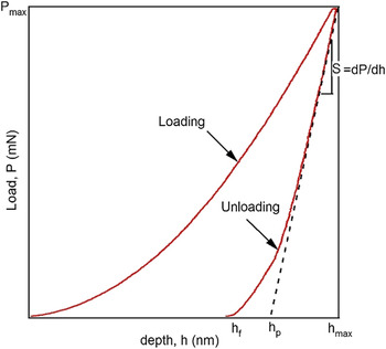
where h p is the plastic depth obtained as the intercept with the displacement axis of the tangent line to the unloading curve at maximum load.
Oliver and Pharr demonstrated that the Doerner and Nix approach presented some inconsistencies, i.e., the measured contact stiffness is highly dependent on the portion of the unloading curve taken for its calculation, the creep phenomenon at the beginning of the unloading curve, and the change in the area during the indenter removal. Reference Oliver and Pharr15,Reference Oliver and Pharr20
On the other hand, the method of Oliver and Pharr is the approach that has been mainly used by the majority of researches related to IIT. In contrast to the method of Doerner and Nix, Oliver and Pharr demonstrated that unloading curves are not well represented by a linear fit. Instead, unloading curves are properly approximated by a power law relationship. This method can be extrapolated to a diversity of axisymmetric indenter geometries such as sphere and pyramids. Reference Oliver and Pharr15,Reference Oliver and Pharr20
This paper is focused on the study of a new approach of the Oliver and Pharr model to fit the unloading curve for pyramidal indenters (Vickers and Berkovich), which is intended to improve the robustness of the method. The study is limited to nanoindentation tests on two materials with very different mechanical behavior, such as fused silica and aluminum.
II. THEORETICAL BACKGROUND
Oliver and Pharr proposed that the unloading curve is generally well approximated to a power law as the following relation [Eq. (2)]:
 $$P = B' \times {\left( {h - {h_{\rm{f}}}} \right)^m}\quad ,$$
where B′, m, and h f are fitting parameters determined by a least squares fitting procedure.
The previous relation is commonly used in the IIT analysis because it generally approximates well the unloading data. Oliver and Pharr did a broad study over different materials and proved that the variation of the power law exponent remains in the range of 1.2 ≤ m ≤ 1.6, which discards the flat punch approximation (m = 1) and approaches instead to a paraboloid of revolution (m = 1.5). This result was unexpected to Oliver and Pharr, because the axisymmetric equivalent to the Berkovich indenter is a cone (m = 2). Reference Oliver and Pharr20 The inconsistency was explained by the concept of “effective indenter shape”, explained in detail in Ref. Reference Pharr and Bolshakov21.
During the initial loading stage of indentation tests, the material is deformed plastically and elastically and the contact impression can be simulated as a perfect cone shape. During the unloading, the indentation imprint changes due to the elastic recovery. Consequently, the unload impression is not perfectly conical, since a small curvature is created on its surface. The effective indenter shape concept accounts for the formation of this curvature. This concept considers the fact that the unloading process is described by a half-space with a local distortion of the surface, caused by the plastic deformation during the formation of the indentation imprint, instead of an elastic contact between a rigid cone and a flat elastic half-space. The elementary idea is to transform the contact geometry to the geometry where the elastic half-space solutions can be applied, to consider the surface distortion. Reference Pharr and Bolshakov21
To compute the elastic modulus and hardness, it is necessary to measure and calculate four principal parameters: the maximum load, P max, the maximum displacement, h max, the final or residual depth, h f, and the contact stiffness, S (dP/dh). P max and h max can be measured directly from the indentation curve, however, S and h f need to be computed. The schematic load–penetration curve obtained by IIT, showing the mentioned parameters, is presented in Fig. 1.
Typical load–depth curve obtained by IIT. P max: maximum load, h max: maximum displacement, h f: residual depth, h p: plastic depth and, S: stiffness.

The hardness, HIT, is defined as the ratio between the maximum load, P max, and the projected contact area, A c,
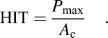 $${\rm{HIT}} = {{{P_{\max }}} \over {{A_{\rm{c}}}}}\quad .$$
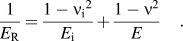
The reduced elastic modulus, E R, is calculated with the contact stiffness as follows:
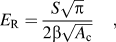 $${E_{\rm{R}}} = {{S\sqrt \pi } \over {2\beta \sqrt {{A_{\rm{c}}}} }}\quad ,$$
where β is a factor related to the geometry of the indenter, for Berkovich indenters commonly is 1.034. Reference Oliver and Pharr20 E R contains the properties of the indenter (E i, νi) and the material (E, ν) described by Eq. (5). For diamond indenters, E i = 1140 GPa and νi = 0.07,
 $${1 \over {{E_{\rm{R}}}}} = {{1 - \mathop {{\nu _{\rm{i}}}}\nolimits^2 } \over {{E_{\rm{i}}}}} + {{1 - {\nu ^2}} \over E}\quad .$$
The contact stiffness is calculated as the slope of the upper portion of the unloading curve; explicitly, it is the derivative of load with respect to the displacement evaluated at the maximum displacement [Eq. (6)], Reference Oliver and Pharr20
 $${S_{{\rm{O\\& P}}}} = {{{\rm{d}}P} \over {{\rm{d}}h}} = mB'{\left( {{h_{\max }} - {h_{\rm{f}}}} \right)^{m - 1}}\quad ,$$
where the subscript O&P for the contact stiffness S denotes that the relation is derived from the Oliver and Pharr model.
The contact area function is a critical quantity to compute, especially in nanoindentation tests with pyramidal indenters, where the influence of the blunted indenter tip can be very important, especially for small displacements. For that purpose, the contact area function proposed by Oliver and Pharr is a good approach [Eq. (7)],
 $${A_{\rm{c}}} = {C_0}\mathop {{h_{\rm{c}}}}\nolimits^2 + {C_1}\mathop {{h_{\rm{c}}}}\nolimits^1 + {C_2}\mathop {{h_{\rm{c}}}}\nolimits^{{1 \mathord{\left/ {\vphantom {1 2}} \right. \kern-\nulldelimiterspace} 2}} + {C_3}\mathop {{h_{\rm{c}}}}\nolimits^{{1 \mathord{\left/ {\vphantom {1 4}} \right. \kern-\nulldelimiterspace} 4}} + \ldots + {C_8}\mathop {{h_{\rm{c}}}}\nolimits^{{1 \mathord{\left/ {\vphantom {1 {128}}} \right. \kern-\nulldelimiterspace} {128}}} \quad .$$
The contact penetration depth, h c, changes according to the predominant deformation mode. Frequently, two methods are used, Oliver and Pharr for sink-in and Loubet et al. Reference Loubet, Bauer, Tonck, Bec, Gauthier-Manuel and Nastasi22,Reference Hochstetter, Jimenez and Loubet23 for pile-up,
 $${h_{{\rm{c}}\_{\mathop{\rm s}\nolimits} {\rm{ink - in}}}} = {h_{\max }} - 0.75{{{P_{\max }}} \over S}\quad ,$$
 $${h_{{\rm{c\_pile - up}}}} = 1.2\left( {{h_{\max }} - {{{P_{\max }}} \over S}} \right)\quad .$$
III. A NEW APPROACH OF THE OLIVER AND PHARR MODEL TO APPROXIMATE THE UNLOADING CURVE
The Oliver and Pharr model is rewritten as a dimensionless relation [Eq. (10)] to get comparable parameters for various tests and loads. Otherwise, the parameter B′ of Eq. (2) changes its units (mN/nm m ) and is not comparable between tests if the power law coefficient, m, takes different values,
 $${P \over {{P_{\max }}}} = B \times {\left( {{h \over {{h_{\max }}}} - {{{h_{\rm{f}}}} \over {{h_{\max }}}}} \right)^m}\quad ,$$
where B is given by the following relationship:
 $$B = B' \times {{\mathop {{h_{{\rm{max}}}}}\nolimits^m } \over {{P_{\max }}}}\quad .$$
Consequently, the stiffness corresponding to the Oliver and Pharr model is described by the following relation:
 $${S_{{\rm{O& P}}}} = {{{\rm{d}}P} \over {{\rm{d}}h}} = m \times B \times {{{P_{\max }}} \over {{h_{\max }}}} \times {\left( {{h \over {{h_{\max }}}} - {{{h_{\rm{f}}}} \over {{h_{\max }}}}} \right)^{m - 1}}\quad .$$
The proposed method is intended to simplify the fitting by the least squares procedure to compute easily the parameters that describe the unloading curve and to obtain more robust results. The new approach, called the inverted methodology, is described by Eq. (13), where the displacement is estimated instead of the load. This is expressed by the following dimensionless relation:
 $${h \over {{h_{\max }}}} = {{{h_{\rm{f}}}} \over {{h_{\max }}}} + G \times {\left( {{P \over {{P_{\max }}}}} \right)^n}\quad ,$$
where G, n, and h f are fitting parameters. These parameters can be arranged to get the equivalent ones of the Oliver and Pharr model, applying the next relationships:
 $$m = {1 \over n};\;B = {1 \over {{G^{{1 \mathord{\left/ {\vphantom {1 n}} \right. \kern-\nulldelimiterspace} n}}}}}\quad .$$
The contact stiffness calculated by this method is obtained by the following relation:
 $${S_{{\rm{inv}}}} = {{{\rm{d}}P} \over {{\rm{d}}h}} = {1 \over {n \times G \times {{{h_{\max }}} \over {{P_{\max }}}} \times {{\left( {{P \over {{P_{\max }}}}} \right)}^{n - 1}}}}\quad .$$
IV. LEAST SQUARES METHOD TO FIT THE UNLOADING CURVE
The method most commonly used to fit an experimental data is the least squares regression [Eqs. (16) and (17)], due to the difficulties of solving equations with other methods, especially for complicated fitting functions. Reference Bevington and Robinson24 The principle of this method consists in minimizing the squares of the offsets between the data and the model. The squares are used instead of the absolute offset values because they can be treated as a continuous differentiable quantity, Reference Brown and Mac Berthouex25
 $$\mathop {{\chi _{{\rm{OP}}}}}\nolimits^2 = \sum\limits_{i = 1}^z {{{\left( {\widehat {{P_i}} - {P_i}} \right)}^2}} \quad ,$$
 $$\mathop {{\chi _{{\rm{inv}}{\rm{.}}}}}\nolimits^2 = \sum\limits_{i = 1}^z {{{\left( {\widehat {{h_i}} - {h_i}} \right)}^2}} \quad ,$$
where
 $\widehat {{P_i}}$
and
 $\widehat {{h_i}}$
are the values of load and displacement, respectively, obtained by the fitting with the Oliver and Pharr and inverted models. These values depend on p number of parameters (z ≥ p); P
i
and h
i
are the experimental values from each data point. This is the general expression for the least squares fitting, emphasizing that with the Oliver and Pharr model we minimize the differences between loads and with the inverted methodology the differences between displacements.
The functions implemented to fit the unloading curve for both models are power law functions that can be linearized by applying logarithm at both sides of the equations, Reference Bevington and Robinson24,Reference Smyth, El-Shaarawi and Piegorsch26 to fit the data by a linear least squares fitting. However, this linearization commonly disrupts the implicit assumption of normal distributed errors. Reference Bevington and Robinson24 Due to this reason, we suggest the use of a nonlinear least squares fitting which allows to compute the coefficients of the predicted model by means of an iterative process until convergence is achieved; namely, the process ends when the difference between reduced chi-square values of two successive iterations is less than a fixed tolerance value. Reference Bevington and Robinson24,27 The convergence principally depends on the type of fit (Newton, Gauss–Newton, Levenberg–Marquardt, etc.), the initial parameters, and the selected model. Reference Madsen, Nielsen and Tingleff28,Reference Gratton, Lawless and Nichols29
The metrology loop in a measuring machine is defined for the force and displacement. If the force sensor works properly, Newton’s third law of action–reaction guarantees that the force uncertainties are of the order of magnitude of the sensor uncertainties. On the contrary, the displacement measure is more delicate, any defect of stiffness in the metrology loop or any defect in the alignment of the sensor regarding the direction of the measurement leads to notable uncertainties. Reference Whitehouse30 Thereby, also many factors such as roughness, initial depth of penetration, contact point, thermal drift, mechanical vibrations, fluctuations of voltage, and frame stiffness could affect the measured displacements in instrumented indentation tests. Reference VanLandingham1,Reference Oliver and Pharr15,Reference Fischer-Cripps31–Reference Fischer-Cripps33
The Oliver and Pharr model to fit the unloading curve assigns the load as the dependent variable and the displacement as the independent variable. The least squares regression generally introduces errors in the dependent variable, y. Then, the error on the independent variable, x, should be negligible. In the real data from experimentation both variables are subject to uncertainties, therefore, the uncertainties on the dependent variable should be a sum of measured errors and the error propagated by the uncertainty in x. Reference Bevington and Robinson24,Reference Peters34 However, in the case where one of the variables presents larger uncertainties with respect to the other, this one should be assigned as the dependent variable and the uncertainties over the other one can be considered as negligible. Thus, the inverted methodology swaps the variables of displacement and load, since the uncertainties are more important in the displacement, assigned as the dependent variable.
V. EXPERIMENTS
The studied materials were fused silica (FQ) and an aluminum alloy (Al). The load–displacement curves were taken from nanoindentation tests in MTS Nano Indenter XP (MTS Nano Instruments, Oak Ridge, Tennessee, USA). Several standard tests at different loads from 20 mN up to 500 mN have been performed, the loading and unloading times were 30 s, and the holding time at maximum load is 15 s. The calibration of the indenter tip was done on fused silica, using the continuous stiffness measurement (CSM) method to compute the coefficients of the contact area according to the procedure of Oliver and Pharr; Reference Oliver and Pharr15 the parameters for these tests were frequency, 45 Hz; harmonic displacement, 2 nm; strain rate target, 0.05 s−1; and maximum displacement, 2000 nm.
In this paper, the contact depth h c is calculated for the fused silica using Eq. (8), because the predominant deformation mode is sink-in, instead for the aluminum sample, h c was computed using Eq. (9), because pile-up is the principal deformation mode, according to previous studies. Reference Oliver and Pharr15,Reference Loubet, Bauer, Tonck, Bec, Gauthier-Manuel and Nastasi22,Reference Hochstetter, Jimenez and Loubet23 Therefore, the contact area is computed using Eq. (7), with the coefficients obtained from the calibration on the fused silica. Finally, the elastic modulus is calculated with the relations described in Eqs. (4) and (5).
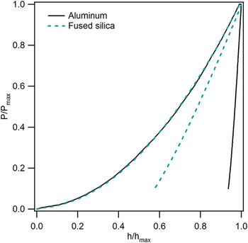
An example of the load–displacement dimensionless curves is presented in Fig. 2 to highlight the dissimilar behavior between the two materials during unloading. The aluminum sample presents a quasilinear behavior.
Load–displacement dimensionless curves for the fused silica and aluminum samples.

VI. COMPARISON BETWEEN THE OLIVER AND PHARR AND THE INVERTED MODELS
The fitting parameters of Oliver and Pharr and inverted models were calculated for the two materials, fused silica and aluminum, to compare these two models.
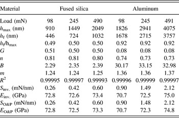
The stiffness and elastic modulus were computed according to the relations previously described using the parameters obtained for each model. Both models were fitted until convergence. The results are presented in Table I, only three loads are represented for convenience to highlight the similitudes between the two methods. Nevertheless, five different loads were used to accomplish the analysis, the tendency related to the fit parameters and the elastic moduli were comparable to the results in Table I. Similar results were obtained in a steel sample.
Fitting parameters obtained by the Oliver and Pharr and inverted models using the dimensionless load–displacement curves.

R 2, coefficient of correlation. O&P: Oliver and Pharr model and inv.: inverted model.
Table I shows that both models lead to a very similar estimation of the stiffness and consequently of the elastic modulus, which is conditioned to the convergence of the fitting of the unloading curves; a more detailed description of this subject is done in the next section. Besides, the two models represent excellently the experimental data since the coefficients of correlation, R 2, between the experimental values and the predicted values are very close to one. Reference Brown and Mac Berthouex25
In general, the inverted approach leads to approximate results of the Oliver and Pharr solution, validating the applicability of this methodology, at least for nanoindentation tests. Therefore, the question is what are the advantages of the inverted approach? The following section gives some elements to answer this question.
VII. FITTING THE UNLOADING CURVES WITH INVERTED AND OLIVER AND PHARR MODELS BY THE LEAST SQUARES METHOD
Most of the instruments compute the stiffness derived from the unloading curve by an internal algorithm that usually approaches the curve to the Oliver and Pharr model. However, sometimes this algorithm can fail, consequently, neither the value of the stiffness nor the elastic modulus is correct. The algorithm can be programmed to a certain number of iterations; therefore, a local minimum can be found instead of a global minimum, obtaining an incorrect result. The evaluation of the results must be done cautiously, if some values of the elastic modulus computed by the software of the instrument are out of the range of coherent values according to the material, then the fitting parameters and the stiffness should be recalculated.
To exhibit the convenience of using the inverted approach to fit the unloading curve as a modified approach of the Oliver and Pharr model, the following assumptions in the data were done that all the measurements have the same standard deviation and that the errors are normally distributed and independent.
Nonlinear least squares fitting needs starting values and step sizes. The rate of the convergence of the approximation method can depend on these parameters and the selected method. An improper selection of the starting point may lead to the solution of a local minimum rather than an absolute one, also several local minimums can exist that render it difficult for the correct selection of the results. In this regard, the Oliver and Pharr model can lead to some problems to achieve convergence if the starting values are not correctly selected, obtaining a local minimum or any solution. Reference Gong, Miao and Peng14 It is worth mentioning that these issues are mainly encountered in metallic samples that present high plastic deformation, rather than in materials with great elastic recovering upon unloading, like fused silica.
As an example of the analysis, the tests of aluminum and fused silica performed at 245 mN load were selected. The algorithm was built in the Mathematica® language to compute the fitting parameters of the unloading curve with both models.
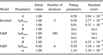
The parameters were computed applying the two models for the fused silica sample. Several methods for the nonlinear fitting were tried: Newton, quasi-Newton, Levenberg–Marquardt, and gradient. The initial values were not introduced in the algorithm, using the values that take Mathematica by default which is one for all the parameters. The Levenberg–Marquardt method leads to convergence with less iterations than the other methods. The Oliver and Pharr model do not achieve convergence with these setup values, the value of h f/h max should be in the same order of magnitude to achieve the convergence (Table II). For the inverted approach, the convergence is reached with five iterations, with the setup initial values. The value of tolerance to stop the algorithm is 0.002, as a default value in Mathematica®.
Fitting results according to the initial values of parameters for the unloading curve of fused silica sample at 250 mN.

nc: without convergence.
In the case of the aluminum sample, the same settings established for the algorithm to fit the curve of the fused silica were applied. An equivalent behavior was obtained, i.e., without assigning initial values in the correct order of magnitude for the Oliver and Pharr model, it is not possible to achieve the convergence (Table III). If the initial values are close to the solution values, the global minimum is easily found; nevertheless, if those are far from the solution, the number of iterations should be increased and in some cases, the convergence is not achieved. The proposed methodology with the default setup values reaches the convergence with 5 iterations. Also, different sets of initials values lead to the same solution. As in the fused silica sample, the best method to perform the least squares procedure is Levenberg–Marquardt for both models.
Fitting results according to the initial values of parameters for the unloading curve of the aluminum sample at 250 mN.

nc: without convergence.
Tables II and III summarize the fitting procedure of the unloading curves for both samples at 250 mN using the Levenberg–Marquardt method with a tolerance of 0.002 using Mathematica®. The fitting procedures were verified with Excel and Igor Pro finding the same trend than with Mathematica®.
The values for the parameters G and n presented in Tables II and III were recalculated using Eq. (14) to find the equivalent parameters of the Oliver and Pharr model, obtaining B = 2.35 and m = 1.27 for the fused silica sample, and B = 33.31 and m = 1.37 for the aluminum sample.
The results presented for the two materials stand out that the convergence is easily reached when the inverted approach is used.
To present some mathematical basis for the previous results, we evocate the conditioning concepts in the numerical analysis. Regarding a function f(x), a well-conditioned problem implies that the small perturbations of x lead to only small changes in f(x). On the contrary, in an ill-conditioned problem a small perturbation of x leads to a large change in f(x), which means that small relative errors in the inputs would lead to high errors in the outputs, opposite to a well-conditioned problem. To quantify the conditioning of a problem, the relative condition number (k) can be computed according Eq. (18). A lower number indicates a better conditioned problem, Reference Trefethen and Bau35–Reference Sofroniou and Spaletta37
 $$k = {{\left\| x \right\|\left\| {J(x)} \right\|} \over {\left\| {f(x)} \right\|}}\quad ,$$
where ‖J(x)‖ is the norm of the Jacobian matrix.
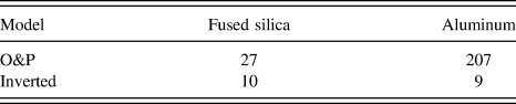
The condition numbers for the Oliver and Pharr and inverted models were calculated using the experimental dimensionless curves at 250 mN for both materials (Table IV). These results are related to the parameters of each model.
Condition number [Eq. (18)] of Oliver and Pharr and inverted models for fused silica and aluminum.
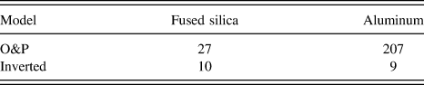
Table IV confirms the results regarding the convergence of the models presented in Tables II and III, indicating that using the inverted approach leads to a better conditioned problem, i.e., small variations in the load data lead to small variations in the displacement data, due to a smaller slope. These results also demonstrate that for metallic samples with a large plastic deformation, as aluminum, the inverted methodology is definitively an improved approach. It is worth mentioning that the relative condition number is only an evaluation of the superior limit of the relative error. Therefore, we evaluate the results in the next section through Monte Carlo (MC) simulations.
A. Testing the robustness of the inverted and Oliver and Pharr models
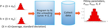
To study the robustness of both models, we used the MC method defined by JCGM 101:2008 38 as “the method used to determine the probability distribution for an output quantity from the probability distributions assigned to the input quantities on which the output quantity depends”. To apply this methodology, the constants of the Oliver and Pharr model computed from the load–displacement dimensionless curves found at 245 mN (Table I) were used to obtain the theoretical unloading curves to being perturbed by a random Gaussian noise. The resulting unloading curves from MC simulations were fitted by the least squares method, collecting 10,000 sets of fitting parameters. The schematic representation of MC simulation is presented in Fig. 3. The initial values to compute the fitting were set up to the approximated values of the solution of the curves without perturbation. The fitting was accomplished using the 80% of the unloading curve according to the standard ISO 14577. 39
Schematic representation of MC simulation, where P and h are the load and displacement of the experimental data at which is added a Gaussian noise centered at zero (average) and standard deviation different to zero (σ).

The random Gaussian noise for the load data is centered at zero with a standard deviation of 0.001 mN. For the displacement, the Gaussian noise is also centered at zero, but the standard deviations (stdv) were fixed at 2.5 nm (∼0.2% h max) and 5 nm (∼0.35% h max) for the fused silica sample, and 2.5 nm (∼0.1% h max), 5 nm (∼0.2% h max) and 10 nm (∼0.35% h max) for the aluminum sample. The purpose is to reproduce the data with high dispersion between the different tests, to evaluate the robustness of the Oliver and Pharr and inverted models.
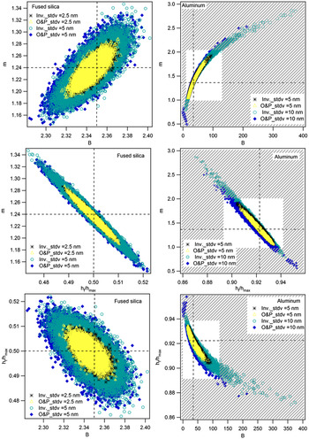
This procedure allows to corroborate the existence of correlations between the parameters of each model, presented in the Fig. 4, showing that the fit constants are highly correlated, as often reported for the power–law correlations. Reference Iost, Guillemot, Rudermann and Bigerelle40,Reference Isselin, Iost, Golek, Najjar and Bigerelle41
Correlation of fitting parameters obtained by the inverted and Oliver and Pharr models. The values are collected from 10,000 load–displacement curves obtained from MC simulation.

Figure 4 clearly shows that increasing the perturbation of the indentation depth leads to a broader dispersion of parameters, which is higher for the aluminum sample.
When the algorithm fails to convergence, another set of parameters can be identified in the plots of h f/h max versus B and m versus B in the aluminum sample given by the Oliver and Pharr model. Nevertheless, the values that are outside of the white squares, under the striped areas, also indicate that the fit performed with both models in the aluminum sample did not achieve the right minimum; the regions were delimited using the bounds of the power law exponent, m, 2 ≥ m ≥ 1, considering that the values out of this range do not have a physical meaning. Reference Oliver and Pharr20 It is consistent that both models sometimes did not lead to convergence because the data are highly perturbed and the procedure of least squares can be easily stacked in a local minimum.
The correlation of fit parameters for the fused silica sample exhibits that both models lead to almost identical results, the region of valuable solutions is just, logically, amplified when increasing the standard deviation of the Gaussian noise on the displacement data. On the contrary, the results for the aluminum samples reveal that the two models do not follow the same trend; this is most notable when the standard deviation is increased. Subsequently, the main arising questions are the following: How these dissimilarities affect the estimation of the stiffness and elastic modulus? Which model would lead to a better approximation of the initial solution?
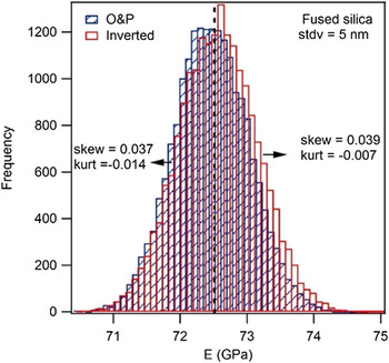
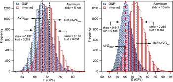
To answer to these questions, we considered the histograms of the elastic modulus of both materials, dismissing the obtained values out of the correct order of magnitude (Figs. 5 and 6).
Histograms of the elastic modulus computed from the curves obtained by MC simulation for the fused silica. stdv represents the standard deviation of the Gaussian noise added to the displacement data. The unloading curves were fitted by the Oliver and Pharr and inverted models.

Histograms of the elastic modulus computed from the curves obtained by MC simulations for the aluminum using the Oliver and Pharr and inverted models. stdv represents the standard deviation of the Gaussian noise added to the displacement data. The dotted lines represent the average elastic modulus of each data (AVGO&P, AVGinv.). For the inverted approach AVGinv., the value matches with the reference modulus (Ref.) computed without perturbation of the data.

The unloading curves for the fused silica sample perturbed with a Gaussian noise with mean 0 and 5 nm standard deviation are perfectly overlapped, indicating that the models of Oliver and Pharr and inverted behave similarly. A smaller noise added to the displacement data results in a similar behavior. Consequently, the estimated elastic modulus computed from the unloading curves using both models leads to similar values, as confirmed by the histograms in Fig. 5.
The histograms representing the elastic modulus of fused silica sample (Fig. 5) corroborate that both models lead to the same results, as observed for the fitting parameters represented in Fig. 4. The average values obtained by the two models are the same as the reference value, 72.5 GPa, and they are well approximated to a normal distribution, i.e., the kurtosis and skewness are almost zero. The introduced noise to the data leads to a range of possible values for the elastic modulus of 72.5 ± 1.7 with 99.73% of probability for the highest noise (5 nm).
The unloading curves of the aluminum sample are similar for both models for the smaller noise of 2.5 nm. However, increasing the standard deviation to 5 and 10 nm causes some dissimilarities between both models, but they are not evident through the illustration of the curves. Nevertheless, the histograms of the elastic modulus obtained by MC simulations (Fig. 6) allow to differentiate between the inverted and the Oliver and Pharr models. There are represented for the Gaussian noise with 5 and 10 nm standard deviation.
The histograms plotted in Fig. 6 confirm the existence of a gap between the results obtained by the two models for the aluminum sample, similarly, to the behavior observed for the fitting parameters in Fig. 4. The mean values obtained by the inverted approach are equal to the reference value, 72.3 GPa. Instead, the average elastic modulus decreases when it is estimated by the Oliver and Pharr model. Likewise, the data obtained by the inverted approach are better approximated to a normal distribution due to the values of kurtosis and skewness are lower than those for the Oliver and Pharr model as presented in the histograms. The values of elastic modulus are summarized in Table V, regarding the different Gaussian noises added to the displacement data.
Elastic modulus obtained by the Oliver and Pharr and inverted models, applying MC simulations with different Gaussian noises added to the displacement data of the aluminum sample.

Results in Table V confirmed the previous statements, i.e., the modulus decreases with respect to the reference value when the Oliver and Pharr model is used to compute it, while the standard deviation of the Gaussian noise added to the displacement data increases.
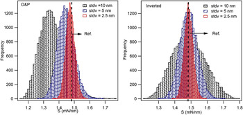
One of the differences in the estimation of the modulus between the two models is related to the computation of the stiffness that includes the residual depth in the Oliver and Pharr model [Eq. (12)], however, it is not considered in the inverted approach [Eq. (15)]. The stiffness depends on the fitting parameters n, m, G, B, and h f/h max, which exhibit differences between them. Generally, the parameters of the inverted approach (n, G, and h f/h max) are closer to a normal distribution in comparison with the parameters of the Oliver and Pharr model (m, B, and h f/h max). These dissimilarities lead to an underestimation of the stiffness when it is computed by the Oliver and Pharr model. The corresponding histograms for the contact stiffness for the aluminum sample are presented in Fig. 7.
Histograms of the contact stiffness, S, computed from the fitting of the unloading curves of aluminum by the inverted and Oliver and Pharr models, for the curves obtained by MC simulation with different Gaussian noises. Ref. is the reference value of S for the curve without perturbation.

Figure 7 shows the diminution of the stiffness computed from the Oliver and Pharr model while the standard deviation of the Gaussian noise increases; this variation of stiffness is directly related to the variation of the elastic modulus (Table V). On the contrary, the stiffness calculated by the inverted approach is centered almost at the same reference value for all the standard deviations, but the normality of the histograms is reduced when the noise increases.
Clearly, the dispersion of the estimated elastic modulus is higher for the aluminum sample than for the fused silica sample, even if the Gaussian noise added to the displacement data is equivalent regarding h max. However, Fig. 2 shows that the unloading curves for the two materials are dissimilar, the slope is higher for the aluminum sample and quasivertical. The gap between the residual depth and the maximum depth that is related to the elastic recovery is 725 nm for the fused silica sample and 226 nm for the aluminum sample. Consequently, an equivalent perturbation of the displacement data would impact more the data of the unloading curve of the aluminum sample because it considers a smaller displacement difference for the fitting, leading to a higher dispersion on the elastic modulus.
According to the previous results, the robustness of the inverted approach to compute the elastic modulus is improved compared to the Oliver and Pharr model, especially for the metallic samples with higher stiffness. For materials with a high elastic recovery, like the fused silica, both models lead to similar results. Nevertheless, if the standard deviation of the Gaussian noise is increased, the fused silica is going to show a similar behavior as the aluminum sample. These results indicate that the designation of displacement as the dependent variable in the model to fit the unloading curve is going to enhance the robustness of the model.
VIII. CONCLUSIONS
The new approach proposed in this paper to fit the unloading curve approximates the experimental data very well and the results are comparable with the Oliver and Pharr model.
The inverted methodology is an approach of the Oliver and Pharr model that proposes the displacement as the dependent variable because this value is more sensitive to large uncertainties than the load, according to one principle of the least squares regression where uncertainties are attributed to the dependent variable.
Generally, the inverted approach facilitates the convergence by a least squares fitting and leads to a better conditioned problem, mainly for metallic samples. If the experimental data are highly perturbed, particularly the indentation depths, the fitting procedure could give a wrong estimation of parameters, finding an incorrect minimum. In this regard, the Oliver and Pharr model is more sensitive. Consequently, by means of MC simulations introducing a random Gaussian noise to the displacement data, we found that the inverted methodology improves the robustness, thus leading to a more accurate determination of the stiffness and the elastic modulus.