Introduction
Slope failure mechanisms along the Antarctic Peninsula continental margin
Slope instabilities along ocean margins are the result of various geological processes such as plate tectonics, eustatic sea level variations, or erosion associated with slope loading. Sedimentary slope failures are the most important trigger mechanism for sediment gravity flows (e.g. turbidites; Løseth Reference Løseth1999).
Turbidites are common deep water deposits (Stow & Mayall Reference Stow and Mayall2000). Turbidity currents can be initiated on slopes by the transformation of slides and slumps into turbulent debris flows as they incorporate more water (Stow Reference Stow1986, Løseth Reference Løseth1999). In numerical experiments using a multi-process sedimentation model, O’Grady & Syvitski (Reference O’Grady and Syvitski2001) showed that the type of mass movement depends on the failed sediment type. Sandy or silty material results in turbidite down-slope transport, whereas clayey materials lead to debris flows. The frequency with which turbidity currents are generated depends on source area, delivery system, slope and seismic activity.
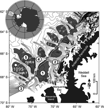
Along the Pacific continental margin of the Antarctic Peninsula, the driving mechanisms for slope loading and failure are erosion of the shelf or hinterland by advancing ice sheets during glacials (Raymond Reference Raymond2002, Dowdeswell et al. Reference Dowdeswell, Ó Cofaigh and Pudsey2004, Bart et al. Reference Bart, Hillenbrand, Ehrmann, Iwai, Winter and Warny2007). The most rapid flow of the West Antarctic ice sheet occurs in areas of ice streams. They occupy glacial troughs, which are observed on the Antarctic Peninsula shelf (Fig. 1 location 1; Pudsey & Camerlenghi Reference Pudsey and Camerlenghi1998, Rebesco et al. Reference Rebesco, Pudsey, Canals, Camerlenghi, Barker, Estrada and Giorgetti2002) and around West Antarctica (Anderson et al. Reference Anderson, Wellner, Lowe, Mosola and Shipp2001). Ice stream flow velocities are typically a few hundred metres per year (Anderson et al. Reference Anderson, Wellner, Lowe, Mosola and Shipp2001). Elverhøi et al. (Reference Elverhøi, Hooke and Solheim1998) compared sediment fluxes of ice streams with the sediment transport efficiency of large fluvial systems and demonstrated that glaciers are far more effective in terms of erosion than rivers. They compiled glacial erosion data from sediment budget and sediment yield studies from the Svalbard–Barents Sea region. According to this study, fast flowing ice streams have the potential to erode terrigenous material at rates more than 1 mm yr-1.
Bathymetric map of the Pacific continental margin off the Antarctic Peninsula. The map shows a glacially driven sediment feeder system of 1) lobes and 2) troughs on the outer shelf, 3) an oversteepened slope, 4) deep sea channels, and 5) sediment drifts on the continental rise and the location of ODP Site 1095 on the distal part of Drift 7 (modified after Lucchi et al. Reference Lucchi, Rebesco, Busetti, Caburlotto, Colizza and Fontolan2002, Rebesco et al. Reference Rebesco, Pudsey, Canals, Camerlenghi, Barker, Estrada and Giorgetti2002).

Along the Pacific continental margin of the Antarctic Peninsula, the grounded ice streams (Fig. 1 location 2) transport eroded terrigenous material over the shelf edge to the over-steepened slope (Fig. 1 location 3; Rebesco et al. Reference Rebesco, Larter, Camerlenghi and Barker1996). Frequent slope failures trigger turbidity currents, which run in channels (Fig. 1 location 4) between large elongated sediment bodies (Fig. 1 location 5) to the abyssal plain. The passage of large turbidity currents through channels (Diviacco et al. Reference Diviacco, Rebesco and Camerlenghi2006) results in spill over silt lamina deposits on twelve sediment bodies along the Antarctic continental rise. These sediment drifts were developed by a complex interplay of down-slope and along-slope processes. The origin of these so called ‘drift bodies’ is still a matter of controversy and depends on the relative importance given to both processes (McGinnis & Hayes Reference McGinnis and Hayes1995, Rebesco et al. Reference Rebesco, Larter, Camerlenghi and Barker1996, Reference Rebesco, Pudsey, Canals, Camerlenghi, Barker, Estrada and Giorgetti2002, Uenzelmann-Neben Reference Uenzelmann-Neben2006).
An exception from the otherwise frequent, small scale glacially controlled turbidite events along the West Antarctic continental margin are two documented, large debris flow deposits between Drift 6 and 7 and within sediment Drift 4 (Fig. 1). These mega flow events are associated with catastrophic continental margin collapse in the late Pliocene (Diviacco et al. Reference Diviacco, Rebesco and Camerlenghi2006, Rebesco & Camerlenghi Reference Rebesco and Camerlenghi2008).
The interaction of ice volume evolution, slope loading and turbidity depositional processes plays a major role in drift build up during glacials and the subsequent deglaciation phase. On the passive and tectonically stable Pacific continental margin of the Antarctic Peninsula, the time interval between slope loading and slope failure mainly depends on slope angle and sediment type. The slope of the outer continental shelf is very steep with an average angle of 16°, making simple slope loading by the ‘ice sheet feeder system’ sufficient to trigger slope failure. This means that local slope instabilities along the Pacific margin of the Antarctic Peninsula are directly linked to regional ice events resulting in turbidity depositions on the drift. Mörz (Reference Mörz2002) showed that the drift bodies represent the most proximal continuous sedimentary recorders for West Antarctic ice events and glacial-interglacial cyclicity.
Organic matter burial and preservation
Organic carbon and biogenic silica (BSiO2) are important components in the marine record. They are used as proxies for West Antarctic palaeoproductivity but are also prone to diagenetic recycling.
The burial efficiency of organic carbon in marine sediments is linked to the marine carbon cycle and plays a major role controlling atmospheric CO2 and O2 (Burdige Reference Burdige2006, pp. 408–441). Several factors control the preservation of organic matter in marine sediments, e.g. organic matter-mineral interactions, organic matter composition and reactivity, and the time of sediment oxygen ‘exposure’ (Burdige Reference Burdige2006). Typical recent open ocean deep sea sediment has organic carbon content as low as 0.3 weight percent (wt%; Stein Reference Stein1990, Burdige Reference Burdige2006). Higher amounts of organic matter preservation require special environmental conditions, e.g. fast burial of organic matter by turbidites (Stein Reference Stein1990). Burdige (Reference Burdige2006) suggests that the organic carbon burial efficiency with respect to the original carbon rain rate to the sediment surface is on average ∼10–20%.
The abundance of BSiO2 in deep sea sediments is often interpreted in terms of productivity pattern of organisms such as diatoms (Koning et al. Reference Koning, Brummer, van Raaphorst, van Bennekom, Helder and van Iperen1997). Biogenic silica or opal is a major component of the skeletal structure of diatoms, radiolaria, silicoflagellates and sponges (Koning et al. Reference Koning, Epping and van Raaphorst2002). Among them, diatoms are the main producers of opal and strongly influence the cycling of silicon and carbon in the oceanic ecosystem (Cortese et al. Reference Cortese, Gersonde, Hillenbrand and Kuhn2004). Smear slides from ODP Site 1095 core sediments show that diatoms assemblages dominate (10–30%) and radiolarians and foraminifers are under-represented (Hillenbrand & Fütterer Reference Hillenbrand and Fütterer2002). The accumulation of biogenic opal on the seafloor is controlled by bioproductivity, dissolution in the water column and diagenetic dissolution within the sediment. Opal preservation after burial is generally very poor. Schlüter (Reference Schlüter1990) determined that in the Weddell Sea, more than 90% of buried opal is dissolved in surficial sediments and released to the sediment-water interface. In general, increased sediment flux leads to faster burial and to better opal preservation (Ragueneau et al. Reference Ragueneau, Tréguer, Leynaert, Anderson, Brzezinski, DeMaster, Dugdale, Dymond, Fischer and François2000).
This study assumes that diatoms are the main carrier of the opal signal (Treguer et al. Reference Treguer, Nelson, Van Bennekom, DeMaster, Leynaert and Queguiner1995), slope loading is dominated by terrigenous material from the shelf and hinterland during glacials, the quantity of diatom fossils settling down from the water column is continuous between two consecutive slope failures, and the laboratory determined leaching rate of biogenic silica from the skeletal structure of diatoms is a function of their diagenetic and transport history.
Regional settings
This study is focused on the early Pliocene sedimentary record from Drift 7, which is one of the largest sediment mounds located south-west of the Antarctic Peninsula (Fig. 1). Its asymmetrical shape, with a short steep side facing south-east and a long, gently sloping side facing north-west, is similar in shape to the other sediment drifts in this area.
The distal part of Drift 7 was drilled by advanced piston corers and extended core barrels from Holes A and B at Site 1095 during ODP Leg 178 (ODP Leg 178 Shipboard Scientific Party 1999). The 561.78 m long composite record covers the late Miocene to the Holocene (∼10 Ma).
Aims of this study
Our study is aimed at quantifying the early Pliocene ice sheet dynamics via slope failure frequencies recorded in Antarctic Peninsula rise sediments. Crucial questions are a) how to determine the average time period between two consecutive turbidite events (turbidite frequency), and b) what other indicators can be used to support the derived model for palaeo ice sheet dynamics. The presented quantification approach of palaeo ice sheet dynamics is a contribution to the question c) how is the Pliocene Antarctic Peninsula ice sheet dynamic forced by Milankovich eccentricity (Grützner et al. Reference Grützner, Hillenbrand and Rebesco2003, Reference Grützner, Rebesco, Cooper, Forsberg, Kryc and Wefer2005, Iorio et al. Reference Iorio, Wolf-Welling and Mörz2004, Hepp et al. Reference Hepp, Mörz and Grützner2006) or does it show autocyclic behaviour (Pudsey Reference Pudsey2002)?
Methods
X-ray images, sedimentary and geochemical analyses from two core intervals of ODP Site 1095 (a: 1095B-10H6 to 1095B-10H3, 171.5–166.5 mcd, lowermost early Pliocene; b: 1095B-4H2 to 1095B-3H4, 108.0–101.0 mcd, uppermost early Pliocene; mcd = revized metre composite depth after Barker Reference Barker2002) were used to reconstruct turbidite recurrence frequencies in order to obtain a measure of the regional palaeo ice sheet dynamics.
Measurements
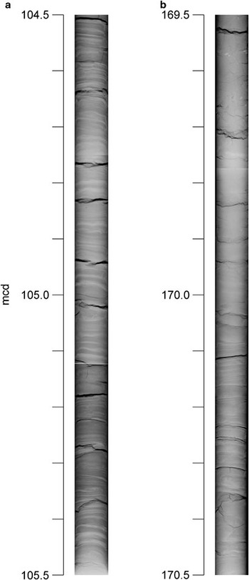
Digital X-ray images (Fig. 2) were made from selected core sections at the Red Cross Hospital, Bremen using ‘Fluorospot compact’ radiography equipment. The dimension of the detector (measuring 40 to 80 cm) determines the size of the single X-ray image. Four overlapping images were produced to cover a 1.5 m core section. Ray penetration of 66 kV and an exposure time of 7.1 mA s-1 were used. The high-resolution images were used to detect and map single silt layers, some of them with distinguishable Bouma sequences. Many of the mapped laminae with a total thickness less than < 1 mm have not been detected before from core images or visual descriptions. A definition of how to best define glacial-interglacial boundaries is given in Hepp et al. (Reference Hepp, Mörz and Grützner2006).
Digital X-ray images from early Pliocene glacial intervals of ODP Site 1095 show the typical, fine laminated silt layer sequences. a. shows core section 1095B-3H6, 104.5–105.5 mcd from uppermost early Pliocene, and b. 1095B-10H5 to 10H6, 169.5–170.5 mcd from lowermost early Pliocene (see Fig. 3).

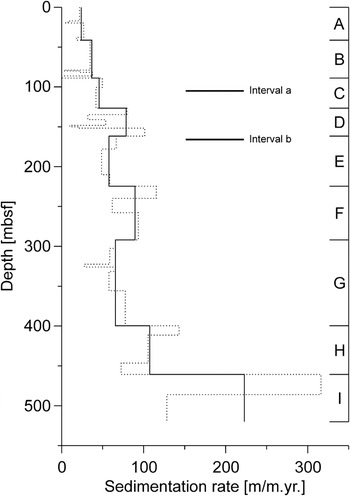
The sedimentation rate (Fig. 3) is based on a magnetostratigraphical-biochronological age model given in Acton et al. (Reference Acton, Guyodo and Brachfeld2002) and Iwai et al. (Reference Iwai, Acton, Lazarus, Osterman and Williams2002; dotted line). The black line shows a simplified linear sedimentation rate model.
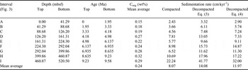
Sedimentation rates (cm kyr-1) for Site 1095 plotted vs depth. The dotted line shows the sedimentation rate based on a linear model from magnetostratigraphical-biochronological tie-points given in Acton et al. (Reference Acton, Guyodo and Brachfeld2002) and Iwai et al. (Reference Iwai, Acton, Lazarus, Osterman and Williams2002). The solid line shows, for this study, a simplified linear sedimentation rate model with intervals A to I. For depth (meter below seafloor = mbsf) and age (Ma) tie-points see Table I. The bars show the depth position of the investigated core intervals (see Figs 2, 4 & 8).

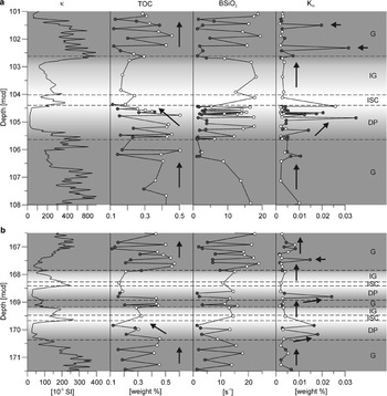
Figure 4 shows parameter of magnetic susceptibility (κ), total organic carbon content (TOC), BSiO2 and the reaction rate constant of leached biogenic silica (Km) from two core intervals, 171.5–166.5 and 108.0–101.0 mcd, of ODP Site 1095 in relation to glacial and interglacial stages proposed by Hepp et al. (Reference Hepp, Mörz and Grützner2006). Magnetic susceptibility (κ) data were obtained during ODP Leg 178 using the shipboard whole-core multisensor track logger (ODP Leg 178 Shipboard Scientific Party 1999). This fast, high-resolution measuring method is used here to distinguish glacial from deglaciation, ice sheet break down and interglacial intervals (see Hepp et al. Reference Hepp, Mörz and Grützner2006). The total organic carbon content (TOC) was measured by LECO on 55 samples. Left over material from the same samples was used to determine the biogenic silica content. The homogenized dry bulk samples were analysed using an automated leaching technique after Müller & Schneider (Reference Müller and Schneider1993) and Km was calculated using a leaching model after Koning et al. (Reference Koning, Epping and van Raaphorst2002, Model 4). The TOC, BSiO2 and Km measurements were distinguished in sediment samples from pure silt layers (Fig. 4, filled circles) and sediments without silt layers (fine fraction <63 μm; Fig. 4, open circles).
Core intervals at a. 108.0–101.0 mcd, and b. 171.5–166.5 mcd of ODP Site 1095. The diagram shows magnetic susceptibility (κ), total organic carbon (TOC), biogenic silica content (BSiO2) and the reaction rate constant of leached biogenic silica (Km), in relation to glacial (G) and true interglacial (IG) stages, as well as deglaciation phases (DP) including the ice sheet collapse (ISC). The sediment samples were distinguished in samples from pure silt layers (filled circles) and sediments without silt layers (open circles). Characteristic gradients of TOC and BSiO2 in relation to glacial stages are marked by arrows.

Relationship of organic carbon and sedimentation rate
In order to determine the average period between two consecutive turbidite events preserved in the silt layer record, glacial-interglacial sedimentation rates were derived from a positive long-term correlation of sedimentation rate and marine organic carbon content.
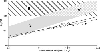
Stein (Reference Stein1990) showed that a positive correlation between organic carbon content and sedimentation rate exists (Fig. 5A and A’), since high sedimentation rates favour the preservation of organic matter by reducing the retention time in the shallow subsurface zone of bioturbation and oxic decomposition. Under anoxic deep bottom water conditions (Fig. 5B) he recognized no positive correlation between organic carbon and sedimentation rate. According to Stein (Reference Stein1990), the relationship between marine organic carbon (Corg) and sedimentation rate (ω, cm kyr-1) in recent sediments can be expressed as a log-linear function:

or

where the factor a is 0.36 and the slope b is 0.64 according to Stein’s (Reference Stein1990) dataset.
Correlation between marine organic carbon and sedimentation rate (modified and simplified after Stein Reference Stein1990). The model is based on data derived from Miocene to Pleistocene/Holocene sediment deposits in open marine (A) oxic, (A’) upwelling high-productivity, and (B) anoxic environments. The symbols and power fit graphs show ODP Site 1095 data of compacted sediments (open rhombi, solid line) and decompacted sediments after Stein (Reference Stein1990) (Eq. (3); filled circles, dotted line) or after Terzaghi (Eq. (4); open circles, dashed line) respectively.

To apply these functions to the relationship between preserved marine organic carbon and sedimentation rate of Pliocene sediments it is necessary to correct the apparent sedimentation rate by a decompaction factor (DF). Stein (Reference Stein1990) proposed the following relationship for the decompacted sedimentation rate (ω 0, cm kyr-1):

where Φ is the mean porosity of the Pleistocene samples in percent and Φ 0 is the porosity of the freshly deposited sediment in the same depositional environment. In this study, the porosity of near surface sediments of ODP Site 1095 was Φ 0 = 75%. For comparison, the average porosity for the Pliocene section is 59%.
A second approach to calculate decompacted sedimentation rates is based on Terzaghi’s one dimensional consolidation theory (Azizi Reference Azizi2000, p. 170, eq. 4.1), restores the original sedimentation rates and is based on the volume independent void ratios:
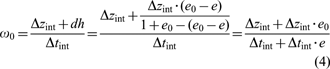
where dh is the height loss by compaction, Δzint is the compacted interval length and Δtint is the time of deposition of each interval; e 0–e is the difference between the initial and the measured void ratio of the compacted sediment as retrieved from the cores.
Mean duration of glacials and interglacials in relation to the deglaciation phase
On the basis of the mean average organic carbon content of each core interval from a composite splice of ODP Site 1095, the long-term correlation (9.8 Ma) between organic carbon and the compacted and decompacted sedimentation rate was calculated using Eqs (3) & (4), respectively. The data is plotted to a log-log scale and fitted by a power function (Fig. 5). The decompacted sedimentation rate is based on a simplified model (Fig. 3, solid line) of the linear sedimentation rate from magnetostratigraphical-biochronological age tie-points given in Acton et al. (Reference Acton, Guyodo and Brachfeld2002) and Iwai et al. (Reference Iwai, Acton, Lazarus, Osterman and Williams2002; Fig. 3, dotted line). The data are given in Table I.

The compacted and decompacted linear sedimentation rates were used to calculate the mean duration of glacials (ΔtavG) between neighbouring magnetostratigraphical-biochronological age tie-points in the time interval from 5.98 to 3.22 Ma (latest Miocene to mid–late Pliocene):

where ΔzavG and ΔzavIG are the mean average length of glacials and interglacials respectively, ΔtavGIG is the mean average period defined by the age tie-points 5.98 Ma and 3.22 Ma (= 2.67 Ma) divided by the number of identified glacial-interglacial cycles (= 22). The linear sedimentation rate ratio (ωav ratio) between glacials and interglacials is calculated from the compacted mean average linear sedimentation rate and decompacted linear sedimentation rates using Eqs (3) & (4).
To further refine the mean duration of glacials and interglacials, a model of three main sedimentary stages within a glacial-interglacial cycle was used (Hepp et al. Reference Hepp, Mörz and Grützner2006): a) Full glacial (G), b) deglaciation phase (DP) including the ice sheet collapse (ISC), and c) ice sheet growth phase, here referred as true interglacial (IG). An example for this model is shown in Fig. 4.
The refinement is necessary since the deglaciation phase was previously unconsidered. This could lead to an inaccurate estimate of the initial, mean average glacial-interglacial interval length and period respectively, because the boundaries of the deglaciation phase are only definable with a complex multi-parameter approach (Hepp et al. Reference Hepp, Mörz and Grützner2006). Deglaciation phases are influenced by a decline in glacial silt deposition and an increase in interglacial organic input.
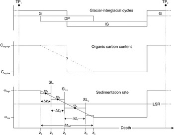
Another problem with using the positive correlation of sedimentation rate and marine organic carbon content arises from the significant diagenetic influence on the organic carbon preservation during the deglaciation phase reported by Hepp et al. (Reference Hepp, Mörz and Grützner2006). The model of organic carbon-sedimentation rate correlation is not suitable to calculate the duration of the deglaciation phase. To limit the uncertainties introduced by the ‘deglaciation phase problem’ a linear decrease of the sedimentation rate from a higher glacial to a lower interglacial level was assumed. A simple glacial-interglacial model with a deglaciation phase spanning equal parts of both depths intervals was used. The duration of the deglaciation phase and the relative timing t(z) of each silt layer (SL) depositions (z) was calculated on the basis of the length in decompacted core meters of the deglaciation phase zDP and glacial and interglacial sedimentation rates ωG, ωIG using the function:

The model is sketched in Fig. 6 and the results are given in Table II.
Schematic diagram of the relationship between glacial-interglacial cycles, changes in the organic carbon content and changes in the sedimentation rate comprising following findings and boundary conditions: 1) The duration of glacial (G) and interglacial (IG) intervals is similar and the deglaciation phase (DP) spans equally both intervals, 2) The mean marine organic carbon content (Corg) correlates positively with the mean sedimentation rate (ω). Both, marine organic carbon contents and sedimentation rate are high in glacials, they decrease during deglaciation phase (glacial to interglacial transition), then achieve a lower level in the upper part of the interglacial and jump again to a high at the interglacial-glacial transition, 3) The linear sedimentation rate (LSR) based on a magnetostratigraphic-biochronologic age model given in Acton et al. (Reference Acton, Guyodo and Brachfeld2002) and Iwai et al. (Reference Iwai, Acton, Lazarus, Osterman and Williams2002) and was computed using the tie-points TP1 and TP2, 4) For the deglaciation phase we calculated the duration and the relative timing of each silt layer (SL) depositions (zn) on the basis of the length of the deglaciation phase (zDP) and the sedimentation rates (ωn) coaxial between two adjacent silt layers (Δzn) using the function given in Eq. (6). Results are given in Table II.

Computation of the mean average period of glacials (ΔtzavG + DP/2) and interglacials (ΔtzavIG + DP/2), each include half of a deglaciation phase, between the magnetostratigraphic-biochronologic age tie-points 5.98 and 3.22 Ma. Given are the results from different models on basis of linear sedimentation rates (see Table I) from (a) compacted sediments and decompaction models after (b) Stein (Reference Stein1990; see Eq. (3)), and (3) Terzaghi (see Eq. (4)). These values were used for Eq. (5).

Leaching rate of biogenic silica (opal-A)
In order to support the derived turbidite frequency data we also looked at opal dissolution parameters as an additional approach to quantify the retention time between two consecutive slope failures. The reaction rate constant from automated leaching methods of biogenic silica, in the following called leaching rate, was used as an indicator for the preservation state of diatom frustules. Exposure times and preservation stage may vary depending on the relative time of the frustules spend for vertical settling through the water column, burial in the sediment or during transport and depositional processes on the continental shelf, slope and rise, respectively.
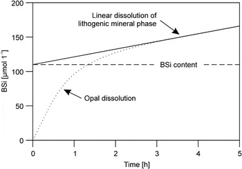
Most of the reactive silica in marine sediments has a biogenic origin (Koning et al. Reference Koning, Epping and van Raaphorst2002). Since the Si-dissolution of BSiO2 occurs independently from dissolution of the lithogenic phase from clay minerals (DeMaster Reference DeMaster2002) it is necessary to distinguish between dissolving biogenic silica and silica from clay minerals. Si-dissolution from clay minerals has a linear and much slower reaction rate than of BSiO2. Corrections for BSiO2 from the lithogenic mineral phase can be achieved by extrapolation of the linear dissolution trend and subtraction from the measured total dissolved BSiO2 (Fig. 7).
Schematic sketch of an opal (BSi) dissolution curve (dotted line). The SiO2 contribution of the lithogenic mineral phase can be extracted by a backward extrapolation of the linear fit of the dissolution curve. The corrected BSi content is retrieved from the fit curve at time zero (modified from Koning et al. Reference Koning, Epping and van Raaphorst2002).

Müller & Schneider (Reference Müller and Schneider1993) proposed an automated alkaline leaching method to determine the biogenic silica content in surface sediments and to discriminate between leached silica from the biogenic fraction and the lithogenic fraction. The digital data of the leaching curves were run through a fitting procedure after Koning et al. (Reference Koning, Epping and van Raaphorst2002, Model 4) to obtain a measure of the biogenic silica reactivity via the reaction rate constant (Km):

where Siextr is the initial extractable Si (μm 1-1), α measures the average lifetime of the extractable components in the mixture and ν is a non-dimensional parameter.
Results
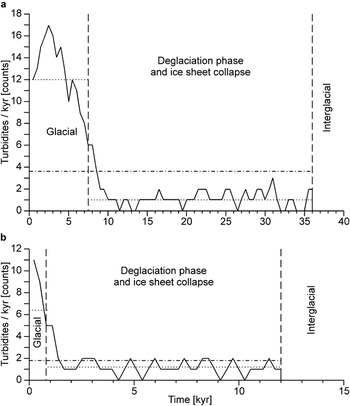
The early Pliocene turbidite frequency for Drift 7 was determined via the calculation of the glacial-interglacial duration, which is based on the organic carbon correlated sedimentation rate model (Fig. 8, Tables I & II). The results from leaching rate measurements of biogenic silica show the interaction of retention time, transport mechanisms and burial rate during glacial-interglacial cycles (Table III).
Early Pliocene turbidite frequency for ODP 1095 core section between a. 105.64–104.02 mcd, and b. 168.93–168.27 mcd. The diagram shows a decrease in turbidite frequency during the deglaciation and the ice sheet collapse phase. The number of turbidites per 1 kyr was plotted on the ordinate. The dotted line shows the mean average turbidite ratio for the glacial interval and the deglaciation phase respectively. The chain line shows the mean average of the total turbidite interval.

Conceptual model for the interplay of retention time of diatom skeletons on the shelf and slope, transport by downslope mass wasting processes, burial rate on the drift and the effects of these three laboratory opal leaching rate under different glacial-interglacial conditions in the Pliocene. A combination of prolonged retention times, fragmentation and relatively fast burial leads to increased laboratory leaching rates.

Positive correlation of organic carbon and sedimentation rate
The mean organic carbon content (0.24 wt%; see Table I) from ODP Site 1095 samples is typical for open ocean deep sea sediments. The compacted and decompacted sediment data (Fig. 5) show that a positive correlation exists between organic carbon content and sedimentation rate. The power fit of the data in a log-log distribution can be described with the function given in Eqs (1) & (2), where for compacted sediments the constant a is 0.9 and b is 0.47, and for decompaction using Eq. (3) or (4)a is ∼0.1 and b is 0.43 or 0.37 respectively.
Compaction-decompaction models
The calculated glacial-interglacial duration (Table II, ΔtavG and ΔtavIG) show differences of up to 7 kyr between the compaction-decompaction models. The glacial-interglacial sedimentation rate ratio of the two models using decompacted sedimentation rates (Eqs (3) & (4); Table II) is very similar. In the following calculation, Model 3, based on decompaction method after Terzaghi, was used since the void ratio conserves the particle mass and is therefore more appropriate to estimate glacial to interglacial material property changes. The derived sedimentation rate ratio of 1.28 (Table II, Model 3) matches the mean average glacial–interglacial thickness ratio of 1.27 suggested in an earlier paper of Hepp et al. (Reference Hepp, Mörz and Grützner2006). The application of Model 3 (Table II), leads to reasonable mean average glacial periods of 63.98 kyr and mean average interglacial periods of 57.38 kyr. The slight asymmetry toward glacial periods is explained by the ice proximity of the core location.
Turbidite frequency
To estimate the frequency distribution of silt layers from ODP Site 1095 cores, the results from Model 3 were integrated with the X-ray derived turbidite counts. The resulting turbidite frequency model (Fig. 6) is based on the following axioms:
a. The glacial-interglacial periodicity is strongly controlled by Milankovitch cycles (Grützner et al. Reference Grützner, Rebesco, Cooper, Forsberg, Kryc and Wefer2003, Iorio et al. Reference Iorio, Wolf-Welling and Mörz2004) and the average proportion of glacial to interglacial time periods follow Model 3.
b. The ice sheet evolution on the shelf is closely coupled to the sedimentary depositional patterns on the drift and changes in the sedimentary supply reflect regional ice sheet advances, retreats and collapses (Hepp et al. Reference Hepp, Mörz and Grützner2006, Bart et al. Reference Bart, Hillenbrand, Ehrmann, Iwai, Winter and Warny2007).
c. The sediments of glacials are strongly dominated by terrigenous supply (turbidites) with high sedimentation rates. The sediments of interglacials are dominated by pelagic settling of biogenic material and terrigenous material derived from ice rafted debris and wind transport with lower sedimentation rates (Hepp et al. Reference Hepp, Mörz and Grützner2006).
d. The linear sedimentation rate computed from magnetostratigraphical-biochronological tie-points given in Acton et al. (Reference Acton, Guyodo and Brachfeld2002) and Iwai et al. (Reference Iwai, Acton, Lazarus, Osterman and Williams2002) corresponds to the mean average sedimentation rate from all glacials and interglacials of the studied Pliocene core section.
e. Excellent preservation of turbidite-derived silt layers exist on the distal part of the drift at ODP site 1095.
On the basis of this conceptual model, the frequency distribution of silt layers for two early Pliocene glacial to interglacial transitions (168.93 to 168.27 and 105.64 to 104.02 mcd) from core sections of ODP Site 1095 was calculated. For these two sections, the average turbidite re-occurrence is ∼375yrs. A moving average with a 1kyr window for the section between 105.64 to 104.02 mcd (Fig. 8a) and a 0.5 kyr window for the section between 168.93 to 168.27 mcd (Fig. 8b) was used to determine frequencies from silt layer reoccurrences.
The resulting graphs (Fig. 8) show a decrease in turbidite frequency during the deglaciation phase and the ISC which correlates to a time interval of reduced terrigenous sedimentation supply as proposed by Hepp et al. (Reference Hepp, Mörz and Grützner2006). Figure 8 shows the mean average number of turbidites per 1 kyr is ∼6.6 turbidites/kyr for glacial intervals and ∼2.8 turbidites/kyr for the deglaciation phase.
Retention time between two consecutive slope failures
In Fig. 4, the total organic carbon (TOC), biogenic opal (BSiO2) content, and the opal leaching rate (Km) of two early Pliocene core sections (171.5–166.5 and 108–101 mcd) are shown. The bulk magnetic susceptibility (κ) aids in differentiating glacial and interglacial stages. All opal data are measured on the fine fraction (< 63 μm) and distinguishes data from sediment samples with silt layers (solid circles) and without silt layers (open circles).
The BSiO2 data show that the general opal content in interglacials (mean average of sediments without silt layers is 15.90 wt%) is slightly higher than in glacials (mean average of silt layers is 2.16 and of sediments without silt layers is 11.35 wt%). Comparing the opal contents with regard to host sediment grain size, we observe a significantly higher opal content in samples without silt layers (2.57–18.19 wt%) than in silt layer samples (1.06–3.93 wt%).
The leaching rate of opal (Km) is independent of the total opal concentration in the sample and shows no significant variances between glacial to interglacial stages. Focused on deglaciation phases (Fig. 4, DP) and the lower part of glacials (Fig. 4, G) the leaching rate from silt layer samples (mean average 0.0089 s-1) diverges from the overall low background rates and sediment (mean average 0.0027 s-1). In Fig. 4a, a gradual increase in leaching rate during the deglaciation phase is observed with the exception of the last three samples with low values, which correlate negatively with the gradual decrease in silt layer frequency (Fig. 8a). The beginning of glacials is characterized by distinct peaks in leaching rate.
Discussion
Close relationship of ice sheet advances, slope loading and frequent slope failure
In the absence of major fluvial systems, the ice sheet is the main driving force behind erosion, transport and deposition of terrigenous material from the continental shelf to the deep sea sediment drifts. Ice thickness, flow velocity and frequency of advances to the shelf edge determine the amount of material transported to the continental slope. The slope angle is another important component determining transportation rate to the rise. The slope angle is determined by the type of transported material (e.g. coarse material from an erosive glacial advance leads to a steep slope; (Rebesco et al. Reference Rebesco, Larter, Camerlenghi and Barker1996).
The current West Antarctic ice sheet is assumed to have the capability of rapidly shrinking, because the grounding line between the continental ice sheet and the floating ice shelves is mostly far below sea level and thus unstable (Bentley Reference Bentley1998, Raymond Reference Raymond2002). In a recent study of ice sheet dynamics controlled by sedimentary processes along the Antarctic Peninsula continental margin, Hepp et al. (Reference Hepp, Mörz and Grützner2006) proposed a highly dynamic early Pliocene ice sheet with abrupt changes in lithology at interglacial to glacial transitions. A conspicuous feature is the abrupt cessation of ice rafted debris (IRD) input and the synchronous onset of frequent silt layer deposition. The factors controlling the rapid interglacial to glacial transition are not completely understood, but rapid ice re-advances to the shelf edge may point towards an ice sheet which does not fully retreat to the shoreline during interglacials.
In view of the glacial-interglacial cyclicity in the Pliocene, the turbidite depositional regime at ODP Site 1095 shows a consistent pattern in silt layer distribution and frequency (Hepp et al. Reference Hepp, Mörz and Grützner2006). In the early Pliocene the silt layers are closely spaced and the reoccurrence frequency is continuously high in glacials. The frequency distribution of silt layers is interpreted to reflect short and rapid but continuing ice advances every ∼375 yrs. This full glacial depositional pattern is followed by a gradual decrease in silt layer frequency during the deglaciation phase. The ice sheet collapse and the ice sheet growth phases within the interglacial intervals contain no silt layers.
The reaction rate constant (Km), determined from the BSiO2 leaching measurements, was used as an indicator of the diagenetic and transport history of the diatom frustules. The rate constant describes the dissolving rate of opal and depends on the texture and preservation stage of diatom frustules and the deposition mode. Large diatom frustules with complex morphology have a more dissolvable surface than smaller and simpler frustule structures (McManus et al. Reference McManus, Hammond, Berelson, Kilgore, Demaster, Ragueneau and Collier1995, Rabouille et al. Reference Rabouille, Gaillard, Treguer and Vincendeau1997). A larger surface of fragmented diatom frustules dissolves faster than intact skeletons. Van der Weijden & van der Weijden (Reference Van Der Weijden and Van Der Weijden2002) demonstrated the dependency of opal dissolution rate on the reactivity of the opal. They showed that both linked processes decrease with increasing burial depth of the biogenic silica matter. Rapid burial under overall high sedimentation rate (e.g. turbidite events) reduces the reaction time and increases the preservation of reactive opal in the sedimentary record, whereas, under low sedimentation rates, long exposure at the sediment-water interface fosters the dissolution of reactive opal. This leads to diatom remnants in the sediment record that show slow reaction rate constants in laboratory leaching tests. Thus, the reaction rate constant (Km) is an indicator for the exposure time or post depositional transport process of biogenic opal from the continental shelf or slope to the drift recorder.
The results from this study suggest that the combined effects of retention time, transport mechanisms and burial rate are sufficient to explain the observed glacial-interglacial patterns in the opal leaching rate constant. High leaching rates result from a combination of long retention times on the shelf or slope, subsequent mechanical size reduction during reworking of the already weakened frustules during turbiditiy transport, and rapid burial. Low leaching rates indicate either short retention times in combination with rapid burial or long retention times in combination with slow burial. An overview of the transport and deposition effects on laboratory opal leaching rate under different glacial-interglacial conditions is given in Table III.
Characteristic gradients of TOC and BSiO2 in relation to glacial stages are marked by arrows in Fig. 4 and will be discussed in the following: low opal leaching rates during glacials point to a dynamic ice sheet during warm Pliocene ice sheet conditions. Periodically advancing and retreating ice streams discharge large amounts of terrigenous material to the continental slope triggering frequent slope failures (7–12 events per kyr; Fig. 8). Contained in every mass wasting are diatom skeletons deposited on the slope and shelf between two consecutive turbidite events. Short retention times on the shelf or slope prevents a dissolution induced weakening of the frustules. Stable frustules in turn have a higher probability to resist mechanical downsizing during turbiditic reworking. Fast deposition on the drift leading subsequently to small dissolution rates in the laboratory. During deglaciation a decrease in turbidite frequency and prolonged exposure times lead to weaker frustules that experience more mechanical downsizing during turbiditic reworking. Together with the fast deposition and burial, reactive opal gets preserved on the drift. The last three turbidites of the deglaciation phase, however, show lower leaching rate constants. These low leaching rates indicate a burial rate below a critical threshold that would be necessary to preserve the reactive opal fraction. In contrast, the interglacials show that long retention times, no turbiditic reworking and low hemipelagic burial rates allow an effective removal of reactive silica. A few peaks in the leaching rate from silt layer samples during the onset of glacials supports our conceptual model (see Table III for details).
Orbital periodicity in the early Pliocene
The investigated area is sensitive to changes in ice sheet volume in West Antarctica and hence allows regional insights. Barker & Camerlenghi (Reference Barker and Camerlenghi2002) showed that the release of glacial sediments is cyclic and orbitally controlled. From early to late Pliocene intervals of Site 1095 cores Iorio et al. (Reference Iorio, Wolf-Welling and Mörz2004) compiled strong short eccentricity periodicities (∼95–125 kyr). This finding corresponds to our results with periodicities at ∼120 kyr. For Pliocene time sections of ODP Site 1095 cores, a forcing by obliquity periodicities at about 50–60 kyr were reported in different studies: Wavelet analyses of petrophysical measurements show periodicities at 56 kyr and 87 kyr (Lauer-Leredde et al. Reference Lauer-Leredde, Briqueu and Williams2002), and power spectra analyses show periodicities at 63 kyr (Pudsey Reference Pudsey2002) and at 50 kyr and 64 kyr (Iorio et al. Reference Iorio, Wolf-Welling and Mörz2004) in magnetic susceptibility and chromaticity parameter a*. Our study indicates that these periodicities are most likely to respond to the glacial or interglacial half-cycles at 61.59 kyr and 59.77 kyr. Thus for the early Pliocene and the regional ice sheet behaviour we suggest that these periodicities do not reflect the combined effect of precession and obliquity periodicities as predicted by Berger (Reference Berger1977), Iorio et al. (Reference Iorio, Wolf-Welling and Mörz2004) and Grützner et al. (Reference Grützner, Hillenbrand and Rebesco2005).
Conclusion
This study was intended to improve the understanding of the interaction of ice sheet dynamics, slope loading slope failure as reflected in turbidity sediment depositions along the Pacific continental margin of the Antarctic Peninsula during the early Pliocene. We have linked the turbidite frequency and the average time period between two consecutive turbidite events to reaction rate constant measurements on reworked biogenic opal to derive an indirect measure of the slope retention times for two core intervals of ODP Site 1095.
By using the long-term sedimentation rate dependency of the marine carbon burial efficiency in Antarctic drift sediments, it was possible to calculate a ratio of glacial to interglacial sedimentation rates for the Pliocene. Pliocene glacial-interglacial periodicities were determined by using sparse magneto and biostratigraphical tie points and counts of glacial and interglacial intervals. Together with the decompacted average length of glacial and interglacials, a set of linear equations for the glacial and interglacials half-periods and thus absolute half-cycle sedimentation rates were calculated. Decompaction following Terzaghi’s one dimensional consolidation theory and a glacial-interglacial ratio of 1:1 for the deglaciation phase worked best in minimising uncertainties in our calculations. The deglaciation phase required a special adjustment because a diagenetic imprint on the organic carbon preservation prevents the organic carbon sedimentation rate correlation approach for the calculation of the duration of the deglaciation phase. Even for this shelf-proximal site the glacial and interglacial half-periods have on average equal durations of 63.98 kyr and 57.38 kyr, respectively. Derived average glacial turbidite recurrences of ∼375 yr are interpreted as short and rapid ice sheet advances at relatively regular intervals resulting in continuous and periodic slope failures in the late Miocene/early Pliocene warm phase.
Frequent turbidite recurrences imply short retention times between slope loading and slope failure. This finding is supported by low reaction rate constants of opal leaching experiments during early Pliocene glacials. A significant increase of the leaching rate from silt layer samples is associated with a decrease of the turbidite frequency during the deglaciation phase. The complex opal dissolution behaviour observed in the laboratory is explained with a conceptual model of opal exposure, transport and burial. The findings from silt layer frequency distribution and biogenic silica leaching rates imply a close interaction between ice sheet dynamics, sediment discharge, slope loading and slope failure.
The ∼120 kyr Pliocene glacial-interglacial periodicities correspond to data from wavelet and power spectra analyses from ODP Site 1095 on the Pacific continental rise of the Antarctic Peninsula. The previously predicted combined effect of precession and obliquity periodicity of ∼60 kyr from magnetic susceptibility data suggest to correspond rather to glacial or interglacial half-cycles respectively.
Acknowledgements
Samples were provided by the Ocean Drilling Program (ODP). We thank the Bremen Core Repository (BCR) team for their kind support. The BSiO2 measurements were carried out at the Alfred Wegener Institute of Polar and Marine Research (AWI) in Bremerhaven. The help of Dr Gerhard Kuhn und Rita Fröhlking during these measurements is greatly appreciated. We thank Jens Seeberg-Elverfeldt for his useful advice for the linear fitting of opal dissolution curves. Some BSiO2 data from individual samples were part of a bachelor thesis by Sophie Fath prepared in our working group. Special acknowledgment goes to Stefan Kreiter (MARUM) for his help with the calculation of the turbidite frequencies. We thank Rüdiger Stein (AWI) for careful reading of our manuscript and we thank Diane Winter and Ellen Cowan for their reviews which improved our manuscript. This research was funded by the German Research Foundation (DFG project MO1059/1 and HE5377/1) and by the MARUM - Center for Marine Environmental Sciences, University of Bremen.