1. Introduction
The resonant flow in the narrow gap between a carrier and a second vessel or a solid terminal often governs operability (Zhao et al. Reference Zhao, Milne, Efthymiou, Wolgamot, Draper, Taylor and Eatock Taylor2018). Near resonance, the potential flow damping is small and viscous effects can provide a significant contribution to the total hydrodynamic damping. Compared with the inviscid response, the viscous effects are typically significantly more challenging to determine, such that the free surface amplitudes at resonance are difficult to predict.
Given the practical importance, numerous studies have been carried out to investigate resonances in narrow gaps between vessels and terminals, as well as in moonpools. These have been approached theoretically, numerically and experimentally (see e.g. Faltinsen & Timokha (Reference Faltinsen and Timokha2015); Zhao et al. (Reference Zhao, Wolgamot, Taylor and Eatock Taylor2017) and Molin et al. (Reference Molin, Zhang, Huang and Remy2018) and references therein). Such studies have demonstrated how the addition of artificial damping to potential flow solutions, or vortex methods, or viscous solvers with high spatial and temporal resolution are generally required for reliable predictions of the resonant amplitudes. However, the underlying complex flow dynamics around the bilge of the ship and within the gap (or moonpool) which underpins the response remains comparatively less understood.
Provided that the edge or bilge is sufficiently sharp and the Reynolds number is not small, flow separation occurs and vortex shedding can be expected to make a dominant contribution to the damping over other viscous effects such as skin friction (Kristiansen & Faltinsen Reference Kristiansen and Faltinsen2008; Feng et al. Reference Feng, Bai, Chen, Qian and Ma2017). In such cases, the flow dynamics is generally considered to be nearly independent of Reynolds number, with the flow separating at the edge and viscosity only affecting the decay of the shed vortices. However, compared with the flow around an isolated edge, such as the case considered by Graham (Reference Graham1980), for instance, a narrow gap presents additional complexities and gives rise to asymmetries between the oscillatory half-cycles. In particular, the confinement of the flow may be expected to influence the displacement of the vortices which can remain close to the hull and affect the separation, but which has seldom been studied.
Experimentalists have pursued various means to investigate gap and moonpool resonance. The problem has often been simplified by generating idealised two-dimensional flow conditions in a wave tank. Kristiansen & Faltinsen (Reference Kristiansen and Faltinsen2008) and Ravinthrakumar et al. (Reference Ravinthrakumar, Kristiansen, Molin and Ommani2019), for instance, used the forced heave response of two rigidly connected hull sections separated by a small gap to study the moonpool problem. The terminal and side-by-side problems have been investigated using fixed hulls positioned either close to a wall (Kristiansen & Faltinsen Reference Kristiansen and Faltinsen2009) or separated by a small gap (Tan et al. Reference Tan, Lu, Tang, Cheng and Chen2019), subjected to surface waves. Fewer studies have been performed in wave basins, which, although potentially enable realistic hull forms or three-dimensional resonances to be investigated (see e.g. Peri & Swan Reference Peri and Swan2015; Zhao et al. Reference Zhao, Wolgamot, Taylor and Eatock Taylor2017), are less amendable to flow visualisation such as particle image velocimetry (PIV) to study the vortex shedding dynamics.
Experimental studies have also served to provide empirical corrections to inviscid models to enable computationally efficient prediction of the free surface responses in narrow gaps or moonpools, which may facilitate parametric studies. As demonstrated by Kimmoun, Molin & Oikonomidou (Reference Kimmoun, Molin and Oikonomidou2011) for a rectangular barge next to a vertical wall, not accounting for flow separation at the bilges results in unrealistically large predictions of the free surface amplitudes when considering the linear diffraction/radiation problems alone. The effect of vortex shedding has typically been treated indirectly within inviscid models by incorporating a fictitious lid in the gap, tuned to provide appropriate (typically quadratic) damping (e.g. Molin et al. Reference Molin, Remy, Camhi and Ledoux2009). Deploying such models in practice, however, requires understanding the universality of the additional viscous correction terms since the data for their determination are generally limited.
The application of viscous or vortex methods is necessary to resolve the underlying flow dynamics and vorticity fields around the bilge and within the gap. Solvers of the unsteady Navier–Stokes equations for three-dimensional multiphase flow have been implemented by Feng et al. (Reference Feng, Bai, Chen, Qian and Ma2017) and Wang et al. (Reference Wang, Wolgamot, Draper, Zhao, Taylor and Cheng2019) for the pure diffraction response for two identical stationary barges in close proximity. However, significant supercomputing resources are required to fully resolve flow separation which in many cases approximates to two-dimensional flow over extensive lengths of the hull. As such, two-dimensional Navier–Stokes computations are more practical to study the problem and determine the flow field over the entire wave tank as demonstrated by Moradi, Zhou & Cheng (Reference Moradi, Zhou and Cheng2015) and Lu et al. (Reference Lu, Tan, Zhou, Zhao and Ikoma2020), for instance. This also avoids possible issues related to the coupling of viscous solvers to capture flow separation with inviscid solutions as pursued by Kristiansen & Faltinsen (Reference Kristiansen and Faltinsen2012) and Ravinthrakumar et al. (Reference Ravinthrakumar, Kristiansen, Molin and Ommani2019). Notably, Lu et al. (Reference Lu, Tan, Zhou, Zhao and Ikoma2020) considered a barge heaving and swaying next to a vertical wall and presented vorticity contours to support the conclusion that vortex shedding around the square bilge dominated the damping of the gap response.
Vortex methods are particularly well suited to predicting flows with well-defined separation points such as sharp-edged bilges. Graham (Reference Graham1980) applied an inviscid, discrete vortex technique to show that the drag coefficient due to the vortex force for oscillatory flow around an infinite right-angled edge at low Keulegan–Carpenter number ( $K_C$) was independent of
 $K_C$. For relatively small gap oscillations where the vortices remain close to the bilge, this would suggest that the damping coefficient is independent of the geometry. A vortex model combined with an inviscid boundary element solution was also used by Kristiansen & Faltinsen (Reference Kristiansen and Faltinsen2008) to study the moonpool problem. While vortex methods omit diffusion and boundary layer separation, their superior computational efficiency compared with models which solve the full Navier–Stokes equations is particularly useful for conducting parametric studies and estimating the vortex contribution to the damping while still encapsulating the rich physics.
To this end, the objectives here are to devise an experiment and appropriate numerical models to study not only the free surface response but also the flow fields around the bilge and within the gap in resonant conditions. Specifically, the intention is to provide new insights into the fundamental flow separation and vortex shedding dynamics and, in turn, the capabilities of PIV and numerical models to investigate the problem and determine the vortex contribution to the hydrodynamic damping. The response associated with regular waves incident to a two-dimensional section of a fixed barge located next to a vertical wall in a wave tank is considered. The set-up is regarded as a suitable analogue to common gap resonance scenarios in practice, such as the side by side offloading from floating liquefied natural gas (FLNG) facilities to liquefied natural gas carriers in the open sea, and appropriate for evaluating the efficacy of PIV and numerical models of varying fidelity.
2. Experiment
2.1. Facility and set-up
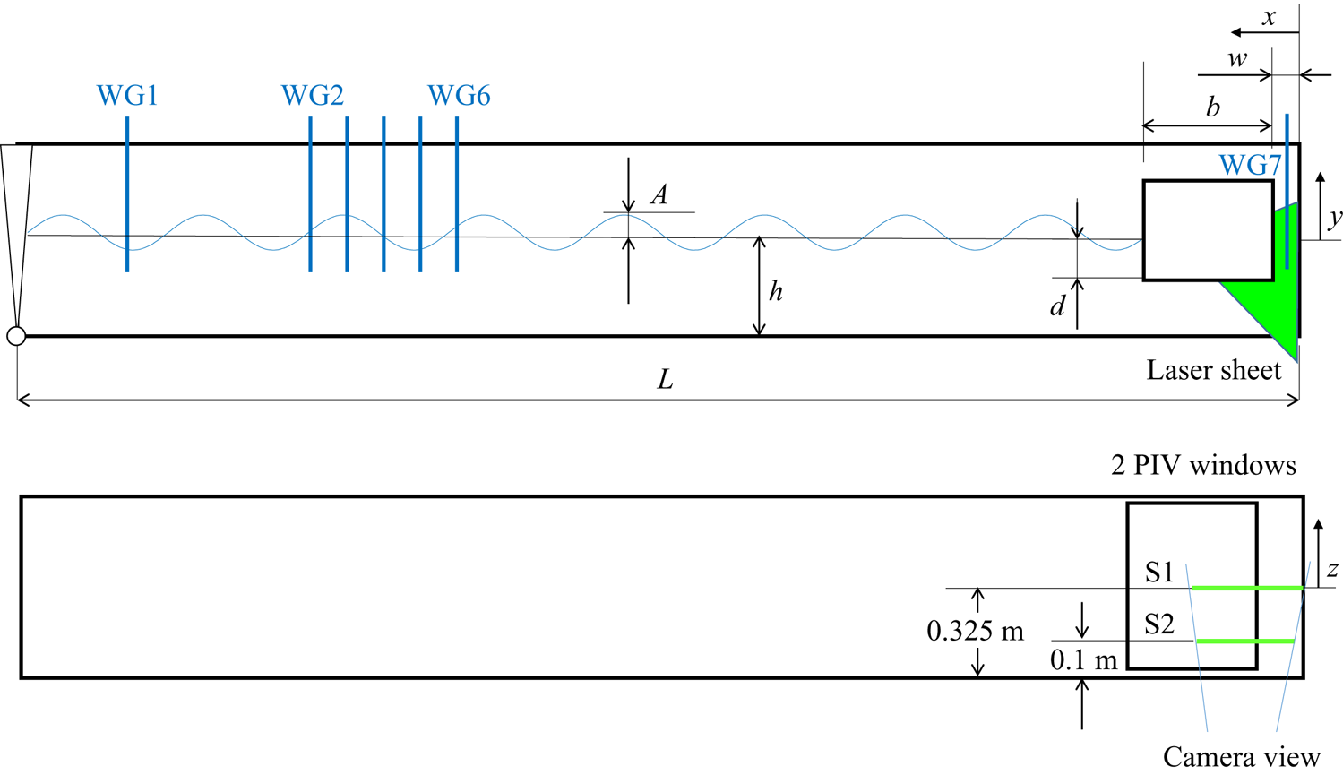
The experiment was conducted in the wave tank at École Centrale Marseille and the set-up is depicted in figure 1. The wave tank is 0.65 m wide and the vertical wall was positioned at a distance of  $L= 12.02\ \textrm {m}$ from the wavemaker, with the water depth set at
 $h= 0.52\ \textrm {m}$. The hull had a beam of
 $b= 0.6\ \textrm {m}$, draft of
 $d= 0.12\ \textrm {m}$ and spanned the width of the tank. The sides of the hull were vertical and the bilges were right angled (i.e. square edges). For the purposes of this study the hull motion was fully restrained and only the pure diffraction response was considered. The vertical wall extended to the bottom of the tank and the gap between the wall and the barge was
 $w= 0.073\ \textrm {m}$ (i.e.
 $w/b=0.12$).
Experimental arrangement in the wave tank.

The barge model was constructed from 250 mm thick polymethyl methacrylate to provide the required rigidity. The vertical wall was a 25 mm thick polyvinyl chloride plate. It was affixed to the walls and bottom of the tank as to ensure that it did not deform under the significant hydrodynamic pressures generated during the experiment. All dimensions and angles were confirmed using a mechanics rule, with tolerances of less than 0.5 mm.
The flat-type wavemaker was used to generate regular surface waves of constant wave steepness. A linear ramp function was applied to the wave amplitude for the first three wave periods in order to reduce the effect of initial transients. All measurements were acquired having ensured that the water in the tank was well mixed and the uniformity of the temperature was confirmed regularly using probes. The water surface elevation was measured at several locations upstream of the barge as well as in the gap using resistance wave gauges. With this set-up, based on a typical wave period of  $T= 1.1\ \textrm {s}$, the reflected wavetrain would be re-encountered at the hull after around
 $t= 35\ \textrm {s}$, providing a sufficient uncompromised test duration.
2.2. Measurement of the flow field
The flow field around the bilge closest to the wall (i.e. within the gap and below) was observed using a PIV system which comprised two 50 mJ lasers pulsed at 100 Hz. The acquisition frequency was set to 200 Hz by adjusting the interval between the two laser pulses. A Phantom V641 camera with a resolution of  $2560\times 1600$ pixels was synchronised with the laser pulses. The water was seeded with silver coated hollow glass spheres of around 10 to 14
 $\mathrm {\mu }$m in diameter.
The vorticity ( $\omega =\partial v/ \partial x-\partial u /\partial {y}$, where u and v are the velocities in the x and y directions, respectively) was computed using an adaptive PIV algorithm based on that described by Thomas et al. (Reference Thomas, Misra, Kambhamettu and Kirby2005). The same algorithm was also applied to compute the vorticity from the velocity data obtained using computational fluid dynamics (CFD) for consistency. The 10-point scheme has the advantage of reducing the effect of fluctuations. A consequence of employing this scheme, however, is that the first two points on the hull wall are subject to a relatively large error. For the smallest discretisation used in the PIV, this affected a region of up to 0.3 mm from the hull wall. The computation of the flow field from the PIV images was also affected by the reflection from the laser sheet onto the hull. As such, it was not possible to reliably compute the flow field in the region of this intense light. This affected a region around 1 mm from the hull, depending on the angle of incidence of the light.
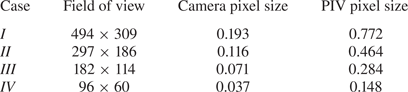
Several fields of view which corresponded to different discretisations (pixel sizes) were tested, as summarised in table 1. For each case, the field was centred on the bilge. Except for the smallest field of view, these images also provided an independent measurement of the free surface in the gap to verify the wave probe measurements. While the majority of the measurements were obtained near the centre of the hull at approximately  $z=0$, where
 $z$ is in the spanwise direction, data were also obtained at
 $z= -0.225\ \textrm {m}$ which allowed for an assessment of spatial variability.
Field of view (width  $\times$ height) and dimensions of the pixels corresponding to the camera images and PIV measurements. All values are in mm.

3. CFD model
The two-dimensional flow field was predicted using a finite-volume solver for the unsteady Navier–Stokes equations and multi-phase flow (i.e. air–water) using direct numerical simulation i.e. with no turbulence model included. Consistent with Lu et al. (Reference Lu, Tan, Zhou, Zhao and Ikoma2020), this was justified based on the flow along the sidewalls of the gap likely being predominantly in the laminar regime. For a typical case with a wave period  $T= 1.1\ \textrm {s}$, such that
 $\varOmega = 5.71\ \text {rad s}^{-1}$ and with the kinematic viscosity
 $\nu = 1.15 \times 10^{-6}\ \textrm {m}^{2}\ \textrm {s}^{-1}$, the viscous length-scale of the Stokes oscillatory boundary layer on both the hull and vertical wall would be expected to be
 $\delta^*=\sqrt{(2\nu/\varOmega)}= 0.6\ \textrm {mm}$. Taking the gap width as a relevant length-scale, a Stokes parameter
 $\beta =w^2/\nu T\approx 4200$ may also be formed. The viscous length-scale of the Stokes layer/gap is
 $\delta ^*/w = (1 - i)\, \textrm {e}^{\textrm {i}\varOmega t}/(2{\rm \pi} \sqrt {\beta })$ which has a maximum value of approximately 0.0025, i.e. a very small portion of the gap. The skin friction is similarly proportional to
 $1/\sqrt {\beta }$ and is very small compared with the pressure drag force from the vortex shedding. Thus this informs the design of the computational mesh, which should be sufficiently fine to capture the vortex shedding while the resolution of the Stokes layers is likely of secondary importance.
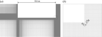
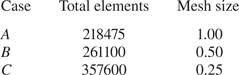
The dimensions of the computational domain were equivalent to the experiment in the  $x,y$-plane. The walls of the hull and exterior domain were set as no-slip boundaries with the upper surface of the domain defined as a pressure outlet. Regular waves were generated at the inlet with a linear ramp function applied to the wave amplitude for the initial three wave periods, as in the experiment. The computations were performed using a fully structured mesh which was refined in the regions of the hull walls, bilges, the vertical end wall and the free surface, as depicted in figure 2. Solutions were attained for three different meshes. These differed between the sizes of the (square) mesh elements which were uniformly distributed within a region of
 $100\ \textrm {mm} \times 100\ \textrm {mm}$ centred on the bilge in the gap, as summarised in table 2.
CFD mesh; (a) in the region of the hull and wall and (b) in the region of the bilge edge in the gap (bounded by dashed lines in (a)).

Total mesh elements in the domain and dimensions of the mesh ( ${\textrm {d} x}={\textrm {d} y}$, mm) within a
 $100\ \textrm {mm}\times 100\ \textrm {mm}$ region centred on the bilge in the gap for the CFD model.

The equations were solved with the widely utilised semi-implicit method for pressure linked equations (SIMPLE) algorithm (Patankar & Spalding Reference Patankar and Spalding1972). The second-order upwind scheme was used for spatial discretisation of momentum and the free surface was tracked using the volume of fluid technique. The computations used a constant time step not exceeding  $T/1000$, where
 $T$ is the wave period. With this, the Courant number was sufficiently low (generally
 $<1$) to ensure simulation accuracy. The free surface time history was extracted at the positions corresponding to the wave gauges in the experiment for comparison with the measurements. The velocity field around the bilge near the wall was sampled at a rate of
 $T/200$ for comparison with the PIV results.
4. Free surface response
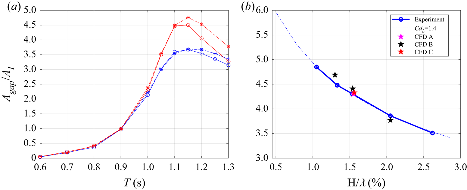
The hydrodynamic response of the free surface in the gap between the hull and wall is first demonstrated, given its central role in driving the vortex shedding around the bilge. Figure 3(a) shows the gap response amplitude operator (RAO) measured by the wave gauge located at the centre of the gap, as a function of the incident wave period. Here, the RAO $\ =A_{gap}/A_i$, where
 $A_{gap}$ is the wave amplitude in the gap and
 $A_i$ is the incident wave amplitude. The results are for constant wave steepness values of
 $H/\lambda \simeq 2 A_i/\lambda = 1.3\,\%$ and 2.6 %, where
 $\lambda$ is the wavelength. The resonant peak of the piston mode at a wave period of around
 $T= 1.15\ \textrm {s}$ is clearly distinguishable, varying weakly with wave steepness. Figure 3(b) plots the RAOs as functions of the wave steepness for a wave period
 $T= 1.1\ \textrm {s}$, thus coinciding close to resonant conditions. The RAO exhibits a decrease with wave steepness at a rate close to
 $(H/\lambda )^{-1/2}$, consistent with a purely quadratically damped response.
Free surface RAOs; (a) as functions of wave period for constant wave steepness of  $H/\lambda = 1.3\,\%$ (red) and 2.6 % (blue), with the dashed line corresponding to the damping-lid model prediction; (b) as a function of wave steepness for
 $T= 1.1\ \textrm {s}$ with results for both the damping-lid model and CFD shown.

The measurements have initially been compared with predictions from a potential flow model with a damping lid in the gap, based on Molin et al. (Reference Molin, Remy, Camhi and Ledoux2009) and applied previously by Kimmoun et al. (Reference Kimmoun, Molin and Oikonomidou2011) and Milne et al. (Reference Milne, Kimmoun, Molin and Graham2020). In the model the inviscid solution is obtained using a matched eigenfunction expansion method and the force applied to the massless lid located at the surface is of the form  $F=-\frac {1}{2}\rho C_{D_L} w|\dot {\eta }|\dot {\eta }$, where
 $\eta$ is the free surface elevation in the gap and
 $\rho$ is the fluid density. Favourable agreement is demonstrated when employing a quadratic damping coefficient of
 $C_{D_L}=1.4$ and neglecting the Stokes attached flow contribution. This coefficient was determined through iterative tuning to achieve a best fit to the RAO vs
 $H/\lambda$ curve and it is emphasised that its value was the same for all wave periods and steepness. The results suggest that the viscous damping coefficient is independent of the oscillatory amplitude in the gap, thus consistent with the
 $K_C^0$ proportionality expected for an infinite isolated right-angled edge (Graham Reference Graham1980). This is discussed further in § 6.
Consideration is now given to the comparisons with the CFD results which have been obtained for  $T= 1.1\ \textrm {s}$ and varying values of steepness. The predicted RAOs are shown to be consistent with the measurements and those attained using the damping-lid model. The results for
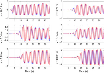
 $H/\lambda = 1.6\,\%$ corresponding to the three different CFD mesh sizes also serve to show that the computations were satisfactorily converged. As a means of further demonstrating the efficacy of the CFD model, the predicted time histories of the free surfaces at various positions along the tank and in the gap for
 $H/\lambda = 1.3\,\%$ are plotted in figure 4. The computed traces are shown to be generally in close alignment with the measurements.
Time histories of the measured (blue) and numerically (CFD) predicted (red) free surface elevation (in cm) at various distances upstream from the vertical wall, for  $T= 1.1\ \textrm {s}$ and
 $H/\lambda = 1.3\,\%$.

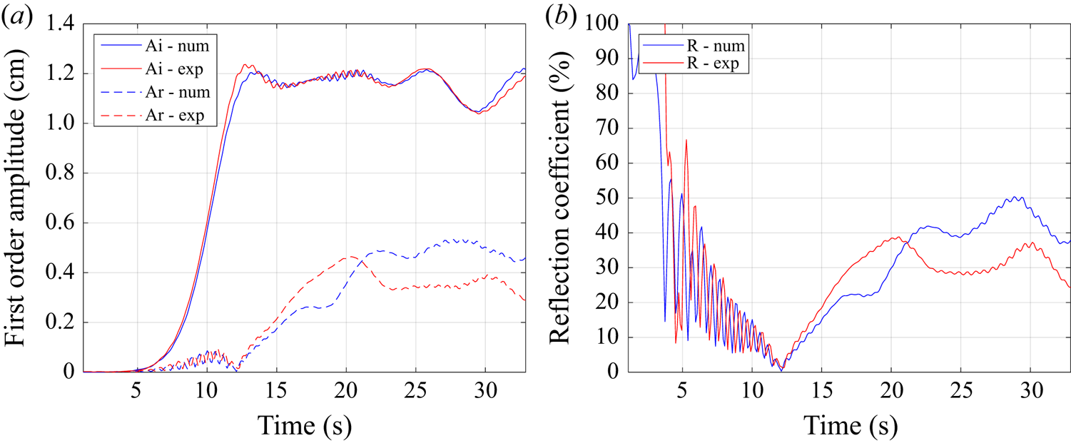
The incident and the reflected amplitudes were subsequently evaluated from both the measured and computed upstream surface elevation data. Here, the technique of Mansard & Funke (Reference Mansard and Funke1980) was applied on moving windows two wave periods ( $2T$) in width with a translation of
 $T/10$. Figure 5 shows the time evolutions of these respective wave amplitudes up to the time in which the wave, having reflected from the hull and then reflected from the wavemaker, re-encountered the first wave gauge. The reflection coefficients are also plotted. These can be related to the dissipation coefficients through energy considerations by
 $K_d = \sqrt {1-K_r^2}$, implying that a significant portion (i.e.
 ${>}90\,\%$) of the wave energy was dissipated. The agreement between the measured and computed incident wave amplitudes provides confidence in having replicated the onset flow conditions. However, the reflected wave amplitude is overpredicted. It is postulated that turbulence which was not explicitly modelled within the numerical solutions, which most likely affects the flow at scales much smaller than those governed by the oscillatory period, may have been a source of the increased dissipation in the experiment.
(a) Time evolution of the incident and reflected wave amplitudes and (b) reflection coefficients, obtained using the separation method for  $T= 1.1\ \textrm {s}$ and
 $H/\lambda = 1.3\,\%$.

5. Vortex shedding dynamics
5.1. Flow around the bilge and in the gap
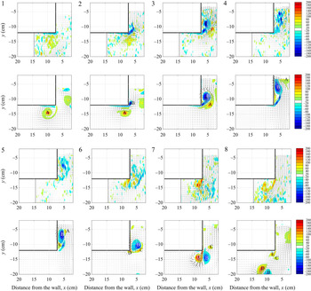
The flow around the bilge next to the wall and in the gap for near resonant conditions is now examined. Figure 6 shows the measured and computed instantaneous vorticity contours and velocity vectors over a single cycle once quasi-steady resonant conditions have been attained (but prior to encountering reflected waves) for  $H/\lambda = 1.6\,\%$ and
 $T= 1.1\ \textrm {s}$. The results are at intervals of
 $T/8$, labelled consecutively, as the flow enters and is then expelled out of the gap. The PIV data are for a pixel size of 0.116 mm (case
 $II$), corresponding to 0.462 mm for the PIV algorithm, with the field of view sufficiently large to visualise the flow up to the free surface. The CFD results are for a mesh size of 1.0 mm (case
 $A$).
Measured (upper panels, for case  $II$) and computed (lower panels, case
 $A$) instantaneous vorticity contours at equivalent intervals of
 $T/8$ (numbered consecutively) during resonance for
 $H/\lambda = 1.6\,\%$,
 $T= 1.1\ \textrm {s}$. The vortex cores are labelled A to E. The extent of the PIV field of view is shown by the dashed lines.

The plots elucidate the inherent complexities in the flow field and the differences compared with shedding around an isolated edge. As the flow enters the gap (occurring between panels 1 and 2) a thin shear layer emanating from the bilge rolls up to form a concentrated counter-clockwise (CCW) vortex core (of negative vorticity and denoted as ‘ $B$’). The CCW vortex pairs with a clockwise (CW) vortex (‘
 $A$’, of positive vorticity) which was shed in the previous half-cycle that has entered the gap with the bulk flow. Owing to the restriction imposed by the narrow gap and the presence of the CW vortex, as the CCW vortex expands it remains near the vertical hull wall (panels 3 to 4). This results in an attached flow away from the edge being induced beneath the primary CCW vortex which is now within a system comprising multiple (negative) vortical regions. The attached flow subsequently separates, generating a secondary CW vortex (denoted as ‘
 $C$’ within panel 5) which initially pairs with core ‘
 $B$’ and convects upward. Without the secondary separation off the surface new positive vorticity would be shed later from the edge when the flow at the edge reverses. As such, here, there is an additional vortex pair (‘
 $B$–
 $C$’) generated within the system.
The residual positive vorticity which remains attached to the vertical wall is subsequently swept to the edge, forming the next CW vortex (‘ $D$’, in panel 7) below the hull as the flow reverses. The proximity of this CW vortex to the hull also induces a local attached flow beneath the hull with relatively weak secondary separation. The primary CCW vortex (‘
 $B$’) is ejected from the gap as the free surface is displaced downward. This vortex now pairs with the CW vortex ‘
 $D$’. The interaction of the vortices, which are of similar but opposite strength, results in a strong local downward velocity below the hull. As the flow reverses again and the free surface moves upward, the CW vortex is reinjected into the gap and the shedding process then repeats. Regions of intense vorticity are present near the hull walls, the thin shear layers and the vortex cores, which are all associated with large flow gradients. Residual vorticity associated with previous shedding cycles is also evident in the flow field, which contributes to the mixing and the decay of the primary vortices.
To demonstrate the consistency of the flow dynamics, figure 7 plots the time histories of the vorticity maxima (both positive and negative) within the field of view and its position relative to the bilge. The corresponding free surface elevation in the gap is also shown for reference. The instances of the most intense positive vorticity are associated with the formation of the concentrated CW vortex core which initially remains just below the bilge. The positive vorticity decreases in strength as the CW core is displaced downward, pairs with the CCW vortex and then moves back upward into the gap. The instances of positive vorticity close to the hull and above the bilge correspond to the local attached flow and the formation of the secondary CW vortex. The secondary separation is also identifiable by the smaller secondary spikes in vorticity maxima time history. Further complexities are exhibited in the negative vorticity. In particular, as the flow enters the gap the maxima alternates between the CCW cores within the multiple vorticial region. Similarly, this gives rise to multiple spikes in the vorticity traces.
Vertical and horizontal positions of the vorticity maxima in the gap measured for case  $II$ (a,c) and computed using mesh case
 $A$ (b,d) for
 $T= 1.1\ \textrm {s}$ and
 $H/\lambda = 1.6\,\%$. The colour range corresponding to the intensity of the vorticity is consistent with figure 6. The free surface elevation in the gap and the edges of the hull are shown by the respective thin and thick solid lines. The vorticity intensity is also shown in panels (a,c) for reference.

5.2. Sensitivity to discretisation
The ability to detect flow features such as shear layers, concentrated vortex cores and secondary separation is inherently dependent on the respective CFD and PIV discretisations. This is of particular concern when assessing convergence and, moreover, comparing numerical and measured results. The effect of discretisation on the CFD results is demonstrated first, using the  $H/\lambda = 1.6\,\%, T= 1.1\ \textrm {s}$ case again. In the computational results, the discretisation changes the capability of the model to describe the physics. Figure 8 shows the traces of the vorticity maxima, together with the surface elevation in the gap, computed using smaller CFD mesh sizes around the bilge of
 ${\textrm {d} x}= 0.50\ \textrm {mm}$ and
 $0.25\ \textrm {mm}$ (i.e. cases
 $B$ and
 $C$). The results are generally consistent with those for the coarser mesh in figure 6. However, the use of a smaller mesh size further elucidates the regions of highly concentrated vorticity close to the hull walls, including those associated with the generation of the secondary vortices.
Vorticity maxima computed in CFD using mesh sizes of 0.50 mm (case  $B$) and
 $0.25\ \textrm {mm}$ (case
 $C$), for
 $T= 1.1\ \textrm {s}$ and
 $H/\lambda = 1.6\,\%$. The vertical positions of the vorticity maxima for the respective cases are shown in panels (a,b) for clarity, with the colour ranges consistent with figure 6. The traces of the free surface elevation in the gap and vorticity intensity are shown in (a,c), for reference, where case
 $B$ is plotted in blue and case
 $C$ in red.

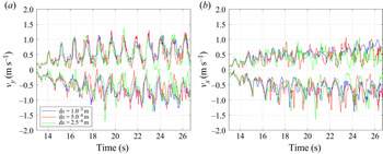
Figure 9 compares the instantaneous vertical and horizontal velocity maxima computed using the three different mesh discretisations. Importantly, as for the free surface responses in the gap, the computed velocities are shown to be in close alignment. The results therefore indicate that the underlying vortex dynamics within the gap associated with the damping has been resolved and reinforces the particular challenge of demonstrating convergence for a gradient quantity such as the vorticity.
Comparison of the computed (a) vertical and (b) horizontal velocity maxima using different CFD mesh resolutions for  $T= 1.1\ \textrm {s}$ and
 $H/\lambda = 1.6\,\%$.

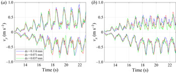
In contrast to the numerical computations, changing the PIV resolution and the field of view modifies the ability to capture the structures while the background physics should be equivalent. The effect of the discretisation on the measured vorticity is demonstrated in figure 10. The larger peaks in the positive vorticity for enhanced PIV resolutions imply greater refinement of the gradients associated with the CW vortex cores below the bilge. The negative vorticity is comparatively less sensitive to the resolution but which is attributed to the thin shear layers and highly concentrated CCW cores within the multiple vortical region which are beyond the limits of the PIV system to resolve. Figure 11 shows that similar to the numerical computations the velocities measured using the different PIV resolutions agree well. However, since the horizontal velocity maxima can occur further away from the bilge compared with the vorticity maxima there are instances (most evident around the secondary peaks) where those results are affected by the differing fields of view.
Comparison of the measured vorticity maxima using different field of views and pixel sizes for  $T= 1.1\ \textrm {s}$ and
 $H/\lambda = 1.6\,\%$.

Comparison of the measured (a) vertical (b) horizontal velocity maxima using different field of views and pixel sizes for  $T= 1.1\ \textrm {s}$ and
 $H/\lambda = 1.6\,\%$.

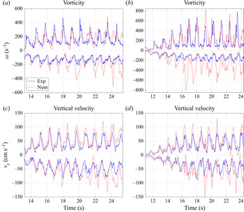
Collectively, these insights are particularly valuable when validating numerical computations using measured data. Direct comparisons of the vorticity and vertical velocity maxima between mesh  $B$ and PIV case
 $III$ and between mesh
 $C$ and PIV case
 $IV$, respectively, are made in figure 12. To facilitate the evaluations, here the CFD results are for a field of view equivalent to the PIV. For these cases, the respective discretisations are shown to have enabled near equivalent resolution of the shedding dynamics associated with the positive vorticity. The limitations of the PIV to fully resolve the features associated with the negative vorticity maxima is again highlighted in the comparisons with the finest CFD mesh. As the negative vorticity in the vortex system is particularly sensitive to the secondary separation, it could, however, be expected that obtaining agreement between the measurements and computations is inherently challenging. The computed and measured velocities, which are less sensitive to both mesh and PIV discretisation, are shown to align closely and provide additional support for having replicated the experiment numerically.
Comparison of the numerical (CFD) and measured vorticity and vertical velocity maxima for  $T= 1.1\ \textrm {s}$ and
 $H/\lambda = 1.6\,\%$. (a,c) PIV with pixels of
 $0.071\ \textrm {mm}$ (case
 $III$) and CFD with a mesh size of
 ${\textrm {d} x}= 0.50\ \textrm {mm}$ (case
 $B$); (b,d) PIV with pixels of
 $0.037\ \textrm {mm}$ (case
 $IV$) and CFD with a mesh size of
 ${\textrm {d} x}= 0.25\ \textrm {mm}$ (case
 $C$).

5.3. Secondary separation mechanisms
Secondary separation which leads to the generation of multiple vortex systems appears to be an attribute of resonant gap flows. It is similar to the secondary separation which is observed under the primary vortices which form above sharp leading edges of delta wing aircraft at high angles of attack (see, e.g. Luckring Reference Luckring2019). As the phenomena have not been reported in oscillatory flows around bilges and other edges, the mechanisms of the secondary vortex separation adjacent to the vertical hull wall are further examined here.
Figure 13 shows the instantaneous vorticity contours and velocity vectors computed in CFD using a mesh sizing of  ${\textrm {d} x}= 0.50\ \textrm {mm}$ (case
 $B$) as the flow enters the gap. The plots thus provide enhanced resolution of the inherent complexities in the vortex shedding compared with figure 6. Specifically, the CW vortex (‘
 $C$’), which is formed following the separation of the attached flow away from the edge, is shown to pair with the primary CCW vortex (‘
 $B$’) with residual vorticity remaining on the hull wall. The pair (‘
 $B$–
 $C$’) initially convects away from the hull and towards the vertical wall and then upwards within the gap, with the CW vortex rotating above the CCW core. The smaller CCW vortex (‘
 $b$’) is instead displaced around the bilge, pairing with the CW vortex ‘
 $D$’ during its formation, before the primary CCW vortex is ejected from the gap. Evidence of the secondary separation and formation of multiple cores is also present in the PIV measurements obtained using
 $0.071\ \textrm {mm}$ pixels (case
 $III$), though notably only part of the primary vortex is able to be visualised within the field of view.
Measured (upper panels, for case  $III$) and computed (lower panels, case
 $B$) instantaneous vorticity contours at equivalent intervals of
 $T/8$ (numbered consecutively) during resonance for
 $H/\lambda = 1.6\,\%$,
 $T= 1.1\ \textrm {s}$. The vortex cores are labelled to be consistent with figure 6, with the smaller cores also identified in lowercase. The extent of the PIV field of view is shown by the dashed lines. The surface pressures (
 $-p_s$ (Pa)) along the vertical hull wall computed in CFD are shown in the insets with key features labelled. The peaks at (i) correspond approximately to the primary CCW core. An adverse pressure gradient exists between (i) and the location of the secondary separation (ii). The CW vortex core associated with the secondary separation is at (iii) and the secondary CCW vortex core corresponds to (iv).

As demonstrated by Hummel (Reference Hummel1979) for a delta wing, the surface pressure distributions also serve to help inform the separation dynamics. The corresponding instantaneous static pressure distributions along the vertical hull wall computed using CFD are also shown in figure 13. The peaks in the suction associated with the primary and secondary vortices are identifiable. Also evident is the region of the adverse pressure gradient which results in the separation of the attached local flow (induced by the primary vortex and directed towards the edge), forming the secondary CW vortex. The displacement of the primary core initially shifts the location of this adverse pressure gradient upward towards the free surface.
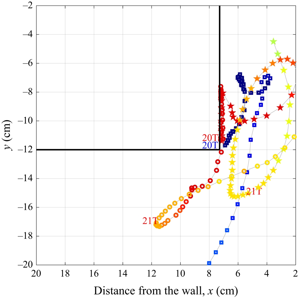
Figure 14 plots the trajectories of the largest vortex structures computed in CFD using  ${\textrm {d} x}= 0.50\ \textrm {mm}$ (case
 $B$) to further illustrate the interactions. Specifically, the primary CCW and CW vortices and the secondary CW vortex have been tracked from their initial formation until they diffuse or are longer visible within the field of view. Their locations at time
 $t=20T$ and
 $21T$, with respect to the start of the simulation, are also indicated for reference. The interaction between the primary CCW vortex and secondary CW vortices, once the latter has formed, is particularly evident. While the primary CCW vortex is ultimately ejected from the gap, the secondary CW vortex reenters the gap and decays within it.


5.4. Self-similarity and spatial invariance
Finally, consideration is given to the variability in the shedding dynamics with the forcing amplitude and along the span of the barge. The spanwise variability, in particular, has seldom been reported for gap resonance studies. The measured vorticity maxima for varying wave steepness, based on a pixel size of 0.071 mm (case  $III$), are compared in figure 15(a). The results demonstrate that the underlying vortex dynamics was generally consistent in the range
 $1.06< H/\lambda \leq 1.62\,\%$, including exhibiting secondary separation. Figure 15(b) plots the vorticity maxima for a relatively large steepness of
 $H/\lambda = 2.6\,\%$. The significant surface amplitudes in the gap necessitate the use of a larger field of view in the PIV (case
 $I$), at the expense of a reduction in the resolution. However, the spatial homogeneity is evident in the comparisons of the measurements which were repeated at the two different spanwise locations. This spanwise spatial invariance also suggests that the process by which the vortex is shed from the bilge is approximately two-dimensional. On this basis, it is postulated that three-dimensionality only becomes significant once the vortices are relatively small in size and are in the process of decaying. Moreover, this provides justification for the application of two-dimensional numerical models when predicting the response.
Measured vorticity maxima for  $T= 1.1\ \textrm {s}$, (a) as a function of wave steepness and (b) as repeated at two different spanwise sections of the barge for
 $H/\lambda = 2.6\,\%$.

6. Resonance response damping due to vortex shedding
The contribution of the vortex shedding to the effective damping of the gap response may be assessed using an inviscid discrete vortex method. This follows the procedure for an isolated sharp edge in oscillatory flow (Graham Reference Graham1980) in which a two-dimensional separated potential flow field due to the shed vortices is calculated as a function of  $z (= x + iy)$ by means of a conformal transformation
 \begin{equation} z = k\zeta^{3/2}, \end{equation}
to the  $\zeta$ half-plane in which k is a matching constant. For a rectangular hull adjacent to a wall this transformation is replaced for the gap and hull edge region by
 \begin{equation} z = z_e + \left[\sqrt{(\zeta/\zeta_e)^2 - 1} - \tan^{{-}1}
\left(\sqrt{(\zeta/\zeta_e)^2 -1}\right)\right]\zeta_e,
\end{equation}
where  $z_e$ is the location of the hull edge relative to the wall at
 $x = 0$, and
 $\zeta _e$ is the point corresponding to the edge in the
 $\zeta$ plane.
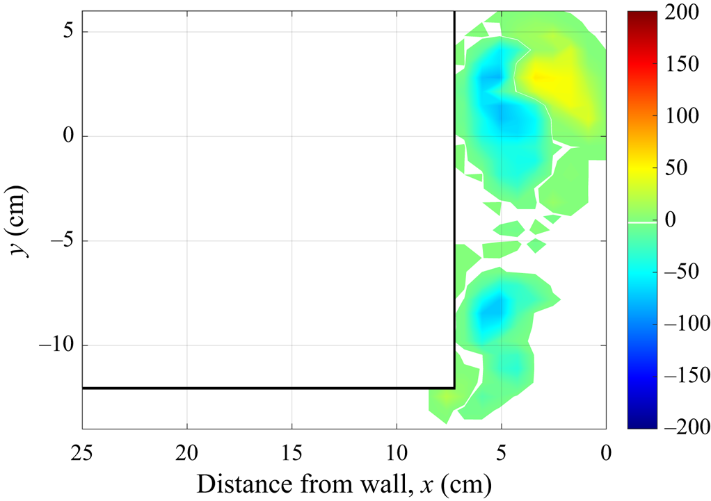
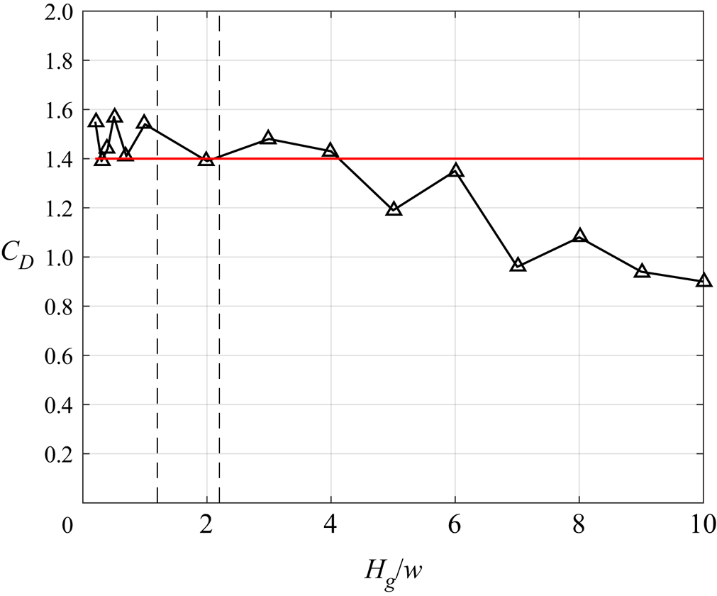
Figure 16 shows an example of the discrete vortex shedding predicted for a given oscillatory flow in the gap, plotted as contours of vorticity on a Cartesian grid. This may be compared with the CFD result shown in figure 6(4). Using this method which is much less computationally intensive a parametric study has been carried out varying the ratio of the gap width  $w$ to the peak-to-trough displacement
 $H_g (= \textrm {RAO} \times H)$ of the free surface in the gap. The damping force
 $F$ acting on the free surface was evaluated as the integral of the component of the excess pressure over the mean free surface due to the shed vortices, in phase with the free surface vertical velocity. The result as a quadratic-damping coefficient (defined as in § 4) is plotted in figure 17 against the ratio
 $H_g/w$. The value of
 $C_D = 1.4$ used in the diffraction computations (§ 4) is marked as a horizontal line while the dashed vertical lines in the plot correspond approximately to the range of values of
 $H_g/w$ in the experiment. The agreement suggests that the vortex shedding is responsible for most of the damping even at the comparatively low Reynolds number of the experiments. The figure also shows how the increasing constraint of the wall as the relative gap width is reduced significantly decreases the vortex generated damping.
Vorticity contour computed using the discrete vortex method, corresponding to resonant conditions at  $t=4T/8$ of a cycle.

Vortex drag coefficient dependency computed using the discrete vortex method. The continuous red line indicates the empirical value of  $C_D$ used for the damping-lid model computations. The range of values of
 $H_g/w$ for the experiment are encompassed by the vertical dashed lines.

7. Conclusion
A new series of wave tank experiments and the application of computational models of varying fidelity have provided new insights into the resonant flow in a narrow gap between a stationary hull and a vertical wall. Vortex shedding from the sharp bilge edge of the hull has been demonstrated to give rise to a quadratically damped free surface response in the gap at resonance. The shedding dynamics was found to exhibit a high degree of invariance to the amplitude in the gap and spatial uniformity along the span of the barge. Secondary separation was also identified as a particular feature of the separated flow at the hull bilge which led to the generation of a system with multiple vortical regions and asymmetries between the inflow and outflow.
The findings can assist in improving or accelerating the computational methods used to predict resonant gap flows and inform offshore operations such as the side by side offloading for FLNG. The influence of discretisation has been demonstrated to be a particularly important consideration when studying the flow dynamics within the gap and comparing flow quantities between PIV and CFD. While it was shown that the instantaneous velocity maxima were well converged both experimentally and numerically, demonstrating convergence and agreement in the gradient quantities such as vorticity is likely to be more challenging. This is attributed to the concentrated vortex cores, thin shear layers and the complexities associated with the secondary separation. The study has also reinforced the value of more computationally efficient semi-empirical models for accounting for the vortex-induced damping in gap flows, provided their limitations are acknowledged. Using both a damping-lid model and a novel application of a discrete vortex method it has been demonstrated that universal quadratic damping coefficients, independent of wave steepness and frequency, may be able to be determined. Such computations are well suited to parametric studies and therefore can be useful for facilitating initial operability assessments, though obviously do not directly model secondary separation.
Funding
This research was supported by the ARC Industrial Transformation Research Hub for Offshore Floating Facilities which is funded by the Australian Research Council, Woodside Energy, Shell, Bureau Veritas and Lloyds Register (Grant No. IH140100012).
Declaration of interest
The authors report no conflict of interest.