1. Introduction
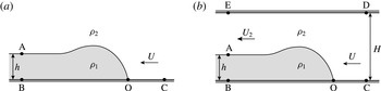
Three-quarters of a century ago, von Kármán (Reference von Kármán1940) introduced the idealized gravity current model shown in figure 1(a). He considered the flow in the reference frame moving with the current front, and invoked three main simplifying assumptions: (i) the flow is steady in this reference frame; (ii) the flow is inviscid; and (iii) the fluid inside the current is at rest. By neglecting the flow in the ambient and applying Bernoulli’s law along the streamlines C–O and O–A, i.e. by assuming that the mechanical energy is conserved along these streamlines, he obtained for the Froude number,
 $$\begin{eqnarray}F_{h}=\frac{U}{\sqrt{g^{\prime }h}}=\sqrt{\frac{2}{{\it\sigma}}}.\end{eqnarray}$$
Here,
 $U$
denotes the front velocity of the gravity current,
 $h$
represents its height,
 $g^{\prime }=g({\it\rho}_{1}-{\it\rho}_{2})/{\it\rho}_{1}$
indicates the reduced gravity, and
 ${\it\sigma}={\it\rho}_{2}/{\it\rho}_{1}$
refers to the density ratio.
Idealized gravity current in a deep ambient (a) and a channel (b).

Benjamin (Reference Benjamin1968) objected to von Kármán’s analysis on the grounds that Bernoulli’s equation should not be assumed to hold along streamline O–A, owing to the dissipation that occurs in this interfacial region as a result of the velocity shear between the current and the ambient, which causes the development of Kelvin–Helmholtz billows and turbulence. Benjamin instead considered a corresponding gravity current in a channel of finite depth
 $H$
, as shown in figure 1(b). By applying the same three simplifying assumptions as von Kármán, and also considering the pressure distributions far up- and downstream of the current front to be hydrostatic, Benjamin was able to write the conservation laws for mass and horizontal momentum flux as
 $$\begin{eqnarray}\displaystyle & UH=U_{2}(H-h), & \displaystyle\end{eqnarray}$$
 $$\begin{eqnarray}\displaystyle & p_{C}H+{\it\rho}_{2}U^{2}H=p_{B}H+{\textstyle \frac{1}{2}}g({\it\rho}_{1}-{\it\rho}_{2})h^{2}-g({\it\rho}_{1}-{\it\rho}_{2})Hh+{\it\rho}_{2}U_{2}^{2}(H-h). & \displaystyle\end{eqnarray}$$
For a given set of values for current thickness, channel height and density ratio, the above relationships represent two equations for the three unknowns
 $U$
,
 $U_{2}$
and
 $p_{B}-p_{C}$
, so that one additional equation is required. To close the problem, Benjamin followed von Kármán’s approach and applied Bernoulli’s law; however, he did so along the bottom wall C–B of the channel, rather than along the interface, as von Kármán had done. For a current of fractional height
 ${\it\alpha}=h/H$
, Benjamin thus obtained for the Froude number,
 $$\begin{eqnarray}\displaystyle F_{H,b}=\frac{U}{\sqrt{g^{\prime }H}}=\left[\frac{{\it\alpha}(1-{\it\alpha})(2-{\it\alpha})}{{\it\sigma}(1+{\it\alpha})}\right]^{1/2}. & & \displaystyle\end{eqnarray}$$
Note that the Froude number
 $F_{h}$
based on the current height is related to the Froude number
 $F_{H}$
based on the channel height by
 $F_{h}=F_{H}{\it\alpha}^{-1/2}$
.
For Boussinesq gravity currents, Borden & Meiburg (Reference Borden and Meiburg2013) showed that invoking an energy closure assumption such as Bernoulli’s equation in Benjamin’s model becomes unnecessary if the conservation of vertical momentum is enforced, along with the conservation of mass and horizontal momentum. This approach bypasses the controversy between Benjamin and von Kármán entirely, as the conservation of energy or head-loss arguments are not required. While there is no flow of vertical momentum into or out of the control volume BCDE, the importance of vertical momentum conservation inside the control volume is clear. The ambient fluid is first accelerated and then decelerated in the vertical direction, which affects the pressure profiles along the top and bottom walls. In turn, these profiles determine the pressure jump
 $p_{B}-p_{C}$
across the current front, for which the need of an additional equation originally arose. Borden & Meiburg (Reference Borden and Meiburg2013) showed that the conservation of vertical momentum can be accounted for by considering the linear combination of the differential versions of the steady-state, inviscid, horizontal and vertical momentum equations, in the form of the Boussinesq vorticity equation,
 $$\begin{eqnarray}\boldsymbol{u}\boldsymbol{\cdot }\boldsymbol{{\rm\nabla}}{\it\omega}=-g^{\prime }\frac{\partial {\it\rho}}{\partial x},\end{eqnarray}$$
where
 ${\it\omega}=\partial v/\partial x-\partial u/\partial y$
denotes the vorticity, and
 $x$
and
 $y$
represent the horizontal and vertical directions, respectively. By integrating (1.5) over the control volume, we obtain a relation governing the total circulation around the control volume,
 $$\begin{eqnarray}\oint {\it\omega}\,\boldsymbol{u}\boldsymbol{\cdot }\boldsymbol{n}\,\text{d}S=\iint -g^{\prime }\frac{\partial {\it\rho}}{\partial x}\,\text{d}A.\end{eqnarray}$$
Equation (1.6) states that, for incompressible flows in the Boussinesq limit, the flow of vorticity into and out of the control volume is balanced by the baroclinic generation of vorticity inside the control volume. For a sharp interface, the area integral of the baroclinic term becomes
 $g^{\prime }h$
. Furthermore, no vorticity enters the control volume, and the flow of vorticity out of the control volume is confined to the vortex sheet between the current and the ambient. The vorticity flux carried by this sheet equals the vortex sheet strength,
 ${\it\gamma}=U_{2}$
, multiplied by the sheet’s principal velocity,
 $u_{PV}=U_{2}/2$
(Saffman Reference Saffman1992; Pozrikidis Reference Pozrikidis1997). Equation (1.6) thus reduces to
 $$\begin{eqnarray}{\textstyle \frac{1}{2}}U_{2}^{2}=g^{\prime }h.\end{eqnarray}$$
Combining the vorticity conservation relationship (1.7) with the continuity equation (1.2) produces
 $$\begin{eqnarray}F_{H,c}=\sqrt{2{\it\alpha}}(1-{\it\alpha}),\end{eqnarray}$$
where the subscript ‘
 $c$
’ refers to ‘circulation model’. Borden & Meiburg (Reference Borden and Meiburg2013) showed that, with regard to the vorticity flux of Boussinesq currents, this relationship between the Froude number and the current height results in better agreement with direct numerical simulation (DNS) results than Benjamin’s relationship (1.4). However, even Benjamin’s model prediction is found to be quite close to the DNS data, which indicates that his zero-head-loss assumption closely approximates the situation in the simulated flow field.
We note that, in the above analysis, the pressure jump
 $p_{B}-p_{C}$
across the current front has become decoupled from the problem of determining
 $U$
and
 $U_{2}$
, which were determined from the conservation of mass and vorticity alone. Up to this point, we have used the conservation of horizontal momentum only in linear combination with the conservation of vertical momentum, i.e. as the vorticity equation. Consequently, if desired, the pressure jump
 $p_{B}-p_{C}$
across the current front can now be determined from the horizontal momentum equation, as was shown by Borden & Meiburg (Reference Borden and Meiburg2013). The decoupling of the pressure in the above analysis is analogous to employing the streamfunction–vorticity formulation of the Navier–Stokes equations, which allows for the numerical simulation of incompressible flow fields without having to calculate the pressure explicitly. As explained earlier, by accounting for the conservation of mass, horizontal and vertical momentum, the above analysis did not have to invoke any assumptions about energy conservation. Rather, individual terms in the energy equation can now be evaluated, so that the overall loss of energy can be calculated a posteriori, rather than assumed a priori.
We remark that both Benjamin’s model and the vorticity model assume that the flow is inviscid. However, the role of viscosity in a real flow affects the two models differently. Benjamin invokes the assumption of inviscid flow in order to apply Bernoulli’s equation to a streamline, along which he expects dissipation to be minimal. We expect that any small amount of viscosity, and hence dissipation, will cause a loss of mechanical energy, so that Bernoulli’s equation will no longer hold exactly. The vorticity model, on the other hand, invokes the assumption of inviscid flow in the context of the vorticity equation, so that it can model the vorticity field as an infinitely thin sheet. A small amount of viscous diffusion in the flow will cause the sheet to attain a finite thickness. However, for the parallel flow field far behind the current front, a small amount of viscosity will not affect the vorticity flux, which remains the same for a thin but finite vorticity layer as it is for a vortex sheet. Hence we would expect the vorticity model to be less sensitive to small amounts of viscosity than Benjamin’s model. The only caveat concerns the stagnation point O, where even a small amount of viscosity might potentially lead to a diffusive loss of vorticity out of the control volume.
As mentioned above, the investigation by Borden & Meiburg (Reference Borden and Meiburg2013) was limited to Boussinesq gravity currents. In the following, we extend their results to non-Boussinesq liquid gravity currents, such as the ones investigated experimentally by Lowe, Rottman & Linden (Reference Lowe, Rottman and Linden2005) and computationally by Birman, Martin & Meiburg (Reference Birman, Martin and Meiburg2005). We will investigate in detail the significance of the three key assumptions invoked by all of the above authors, viz. steady-state flow, inviscid flow and gravity current fluid at rest.
2. Non-Boussinesq gravity currents: theory
In the following, we will present two alternative ways of extending the above analysis to liquid non-Boussinesq flows. The first approach, which more closely follows the work of Borden & Meiburg (Reference Borden and Meiburg2013) by focusing on the vorticity variable, will consider the problem under the standard assumptions of steady-state inviscid flow, with the gravity current fluid at rest. The second, alternative, approach starts from the conservative form of the momentum equations for primitive variables. It will be shown that, with this approach, it is possible to relax some of the standard assumptions. The relationship between the two approaches will be discussed briefly towards the end of the section.
2.1. Vorticity approach
In order to extend the modelling approach by Borden & Meiburg (Reference Borden and Meiburg2013) to non-Boussinesq gravity currents, we begin with the steady-state Euler equation,
 $$\begin{eqnarray}\boldsymbol{u}\boldsymbol{\cdot }\boldsymbol{{\rm\nabla}}\boldsymbol{u}=-\frac{1}{{\it\rho}}\boldsymbol{{\rm\nabla}}P+\boldsymbol{g}.\end{eqnarray}$$
By taking the curl, we obtain the steady-state, inviscid, non-Boussinesq vorticity transport equation,
 $$\begin{eqnarray}\boldsymbol{u}\boldsymbol{\cdot }\boldsymbol{{\rm\nabla}}{\it\omega}=-\boldsymbol{{\rm\nabla}}\times \left(\frac{1}{{\it\rho}}\boldsymbol{{\rm\nabla}}P\right).\end{eqnarray}$$
Integrating over the control volume and using the divergence theorem on the left-hand side yields an expression analogous to the Boussinesq case (1.6),
 $$\begin{eqnarray}\oint {\it\omega}\,\boldsymbol{u}\boldsymbol{\cdot }\boldsymbol{n}\,\text{d}S=-\iint \boldsymbol{{\rm\nabla}}\times \left(\frac{1}{{\it\rho}}\boldsymbol{{\rm\nabla}}P\right)\,\text{d}A~=-\int \frac{1}{{\it\rho}}\boldsymbol{{\rm\nabla}}P\boldsymbol{\cdot }\text{d}\boldsymbol{l}.\end{eqnarray}$$
The final integral is a contour integral along the boundary taken in the positive sense. Unlike the Boussinesq version of the problem, the pressure no longer decouples from the vorticity transport equation. However, since the density is taken to be piecewise constant, in each layer we may take the density out of the integral and reduce the right-hand side of (2.3) to
 $({\it\rho}_{2}^{-1}-{\it\rho}_{1}^{-1})(P_{O}-P_{A})$
, which depends only on the difference in pressures between
 $\text{O}$
and
 $\text{A}$
. Taking the fluid in the current to be at rest leads to
 $P_{O}=P_{B}=P_{A}+{\it\rho}_{1}gh$
. We have not assumed anything about the pressure distribution in fluid
 $2$
upstream or downstream.
From (2.3), we thus obtain for non-Boussinesq currents,
 $$\begin{eqnarray}\oint {\it\omega}\,\boldsymbol{u}\boldsymbol{\cdot }\boldsymbol{n}\,\text{d}S=\frac{g^{\prime }h}{{\it\sigma}}.\end{eqnarray}$$
As for the Boussinesq case, there is no vorticity flux entering the control volume and the vorticity leaving the control volume is confined to a vortex sheet with strength
 $U_{2}$
and principal velocity
 $U_{2}/2$
. The vorticity balance can then be written as
 $$\begin{eqnarray}\frac{1}{2}U_{2}^{2}=\frac{g^{\prime }h}{{\it\sigma}}.\end{eqnarray}$$
Combining this with the continuity equation produces an expression for the Froude number,
 $$\begin{eqnarray}F_{H,c}=\sqrt{\frac{2{\it\alpha}}{{\it\sigma}}}(1-{\it\alpha}).\end{eqnarray}$$
In the limit of small density contrasts,
 ${\it\sigma}\approx 1$
, so that the Boussinesq result is recovered.
2.2. Primitive variables approach
Alternatively, we can begin with the steady-state, two-dimensional Euler equation in conservative form,
 $$\begin{eqnarray}\boldsymbol{{\rm\nabla}}\boldsymbol{\cdot }({\it\rho}\boldsymbol{u}\boldsymbol{u})+\boldsymbol{{\rm\nabla}}P={\it\rho}\boldsymbol{g},\end{eqnarray}$$
where
 $y$
is the vertical direction, so that
 $\boldsymbol{g}=(0,-g)$
and the velocity vector has components
 $\boldsymbol{u}=(u,v)$
. We also assume that
 $\boldsymbol{{\rm\nabla}}\boldsymbol{\cdot }\boldsymbol{u}=0$
. Taking the
 $z$
component of the curl of this equation gives a scalar equation that can be written as the divergence of a vector field,
 $$\begin{eqnarray}L=\boldsymbol{{\rm\nabla}}\boldsymbol{\cdot }\boldsymbol{q}=\boldsymbol{{\rm\nabla}}\boldsymbol{\cdot }\left(\begin{array}{@{}c@{}}g{\it\rho}+\partial _{x}({\it\rho}uv)+\frac{1}{2}\partial _{y}[{\it\rho}(v^{2}-u^{2})]\\ -\partial _{y}({\it\rho}uv)+\frac{1}{2}\partial _{x}[{\it\rho}(v^{2}-u^{2})]\end{array}\right)=0.\end{eqnarray}$$
After integrating over the control volume BCDE and applying the divergence theorem, we are left with integrals over
 $q_{y}$
along the top and bottom walls, and integrals over
 $q_{x}$
along the in- and outflow boundaries. Along the top and bottom walls, we have
 $v=0$
, so that
 $$\begin{eqnarray}q_{y}=-{\it\rho}u\partial _{y}v-{\it\rho}u\partial _{x}u-{\textstyle \frac{1}{2}}u^{2}\partial _{x}{\it\rho}=-{\textstyle \frac{1}{2}}u^{2}\partial _{x}{\it\rho},\end{eqnarray}$$
where the last equality follows from
 $\boldsymbol{{\rm\nabla}}\boldsymbol{\cdot }\boldsymbol{u}=0$
. Along the top, there are no density gradients, so that the last term is zero. Along the bottom, if
 $x=0$
denotes the front location, the velocity in the vicinity of the front will scale as
 $u\propto U\sqrt{x/h}$
. This was shown first by von Kármán (Reference von Kármán1940) for the flow in the ambient, assuming that the current was stationary, and later extended by McElwaine (Reference McElwaine2005), who demonstrated that it also holds in the current. We expect the local density profile near the front to be approximately of error function shape,
 ${\it\rho}=({\it\rho}_{1}+{\it\rho}_{2})/2-({\it\rho}_{1}-{\it\rho}_{2})\,\text{erf}(x/W)/2$
, where
 $W$
is a (small) width. Multiplying this by the velocity and integrating gives a contribution proportional to
 $({\it\rho}_{1}-{\it\rho}_{2})U^{2}W/h^{2}$
for the right-hand side of (2.9), which is small provided that
 $W$
is much less than the current height
 $h$
.
Along the in- and outflow boundaries, we have the
 $q_{x}$
term to consider. When integrating, we can use
 $v=0$
along the top and bottom walls to obtain
 $$\begin{eqnarray}\displaystyle \int _{0}^{H}q_{x}\,\text{d}y & = & \displaystyle g\int _{0}^{H}\!{\it\rho}\,\text{d}y+\int _{0}^{H}\partial _{x}({\it\rho}uv)\,\text{d}y-\left.\frac{1}{2}{\it\rho}u^{2}\right|_{0}^{H}.\end{eqnarray}$$
This result is general in the sense that it holds for any density field, as well as any divergence-free velocity field such that
 $v$
vanishes on the upper surface.
We now limit ourselves to flows in which
 $W/h$
is small, so that the
 $\int \!q_{y}\,\text{d}x$
contribution discussed above is negligible. Furthermore, we assume that
 $\partial _{x}({\it\rho}uv)=0$
sufficiently far in front of and behind the front. The implications of this assumption will be discussed in more detail below.
The shapes of the inflow and outflow velocity profiles are not important since, when we integrate, only the top and bottom values contribute. The driving term is then seen as the difference in the integral of density between the inflow and outflow boundaries:
 $$\begin{eqnarray}g\int _{0}^{H}[{\it\rho}_{BE}(y)-{\it\rho}_{CD}(y)]\,\text{d}y=\frac{1}{2}[u_{E}^{2}{\it\rho}_{E}-u_{B}^{2}{\it\rho}_{B}-u_{D}^{2}{\it\rho}_{D}+u_{C}^{2}{\it\rho}_{C}].\end{eqnarray}$$
In the case considered in detail in this paper, we have
 $u_{E}=U_{2}$
,
 $u_{B}=0$
and
 $u_{D}=u_{C}$
, so that
 $$\begin{eqnarray}gh({\it\rho}_{1}-{\it\rho}_{2})={\textstyle \frac{1}{2}}U_{2}^{2}{\it\rho}_{2}.\end{eqnarray}$$
For general velocity profiles but piecewise-constant density, (2.11) yields
 $$\begin{eqnarray}\displaystyle & \displaystyle {\it\rho}_{2}[Hg-{\textstyle \frac{1}{2}}u_{D}^{2}+{\textstyle \frac{1}{2}}u_{C}^{2}]={\it\rho}_{2}[(H-h)g-{\textstyle \frac{1}{2}}u_{E}^{2}]+{\it\rho}_{1}hg, & \displaystyle\end{eqnarray}$$
 $$\begin{eqnarray}\displaystyle & \displaystyle u_{E}^{2}-u_{D}^{2}+u_{C}^{2}=2hg({\it\rho}_{1}/{\it\rho}_{2}-1)=2hg^{\prime }/{\it\sigma}. & \displaystyle\end{eqnarray}$$
When
 $u_{D}=u_{C}$
, this relation gives a Froude-number condition,
 $$\begin{eqnarray}F_{H,c}=\sqrt{\frac{2{\it\alpha}}{{\it\sigma}}}(1-{\it\alpha}),\end{eqnarray}$$
which is identical to the result obtained with the vorticity approach (2.6). However, in the case when
 $u_{D}\neq u_{C}$
, there is no natural choice for the front velocity to define the Froude number.
The result can be extended to integration along a streamline rather than just
 $y=0$
or
 $y=H$
. Integrating from A to B to C and then back along a streamline just outside the current to A gives
 $$\begin{eqnarray}u_{A}^{2}=2hg^{\prime }.\end{eqnarray}$$
This suggests that perhaps the best measure of velocity to use is actually the velocity
 $u_{A}$
taken just outside the current.
The above analysis holds for general input and output velocity profiles. Details regarding the extension of the primitive variables approach to three-dimensional flows are presented in appendix A.
In the following, we analyse the implications of assuming
 $$\begin{eqnarray}\int _{0}^{H}\frac{\partial }{\partial x}({\it\rho}uv)\,\text{d}y=0\end{eqnarray}$$
in the above derivation. Consider the inviscid, steady-state, vertical momentum equation in conservative form,
 $$\begin{eqnarray}\frac{\partial }{\partial x}({\it\rho}uv)+\frac{\partial }{\partial y}({\it\rho}v^{2})=-\frac{\partial P}{\partial y}-{\it\rho}g,\end{eqnarray}$$
and integrate from C to D, using
 $v_{C}=v_{D}=0$
,
 $$\begin{eqnarray}\int _{C}^{D}\frac{\partial }{\partial x}({\it\rho}uv)\,\text{d}y+({\it\rho}_{D}v_{D}^{2}-{\it\rho}_{C}v_{C}^{2})=(P_{C}-P_{D})-{\it\rho}_{2}gH.\end{eqnarray}$$
This demonstrates that the assumption (2.17) corresponds to requiring that
 $P_{C}$
and
 $P_{D}$
are hydrostatic relative to one another. Corresponding considerations apply to the outflow boundary, provided that
 $v_{A}=0$
, i.e. that the interface at the outflow boundary is flat.
3. Numerical simulations
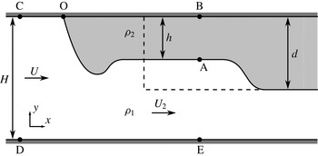
Schematic of a non-Boussinesq lock-exchange gravity current. The Navier–Stokes simulations focus on the buoyant current along the top wall, which more closely corresponds to a quasi-steady flow in the moving reference frame than a negatively buoyant bottom current.

In order to assess the relative accuracy of Benjamin’s and the vorticity model, we compare their predictions to two-dimensional Navier–Stokes simulations of lock-exchange gravity currents. The set-up of the simulations is shown in figure 2, with the dashed line indicating the initial lock configuration. If the lock depth
 $d$
is equal to (less than) the height
 $H$
of the domain, the resulting flow is referred to as a full-depth (partial-depth) current.
During each simulation, one positively buoyant current is generated that propagates to the left along the top wall, and one negatively buoyant current propagates to the right. For full-depth locks, this negatively buoyant current has the form of a gravity current along the bottom wall, whereas for partial-depth locks, it is a bore travelling along the density interface. As will be seen below, the light current along the top wall generally can be approximated more accurately by a quasi-steady flow in the reference frame moving with the current tip, so that it will be more suitable for assessing the validity of the various models. For light currents, Benjamin’s analysis yields
 $$\begin{eqnarray}F_{H,b}=\frac{U}{\sqrt{g^{\prime }H}}=\left[\frac{{\it\alpha}(1-{\it\alpha})(2-{\it\alpha})}{1+{\it\alpha}}\right]^{1/2},\end{eqnarray}$$
instead of (1.4) for dense currents, while the vorticity model results in
 $$\begin{eqnarray}F_{H,c}=\sqrt{2{\it\alpha}}(1-{\it\alpha}),\end{eqnarray}$$
rather than the corresponding relationship (2.6) for dense currents.
3.1. Governing equations
We follow the simulation approach of Birman et al. (Reference Birman, Martin and Meiburg2005) and employ the incompressible, non-Boussinesq, Navier–Stokes equations in two dimensions. As long as there is minimal diffusion, the velocity field can be considered divergence-free, as the flow consists of two separate incompressible fluids. For a discussion of the effects of diffusion on the continuity equation and their quantitative assessment, we refer the reader to Chen & Meiburg (Reference Chen and Meiburg2002). The dynamic viscosities of the two fluids are taken to be equal, and the density field evolves based on a convection–diffusion equation. To minimize mixing, we employ small diffusivities. Referring to figure 2 and letting an asterisk denote a dimensionless quantity, we non-dimensionalize the equations with the lock height
 $d$
, the buoyancy velocity
 $U_{b}=\sqrt{g^{\prime }d}$
, where
 $g^{\prime }=g({\it\rho}_{1}-{\it\rho}_{2})/{\it\rho}_{1}$
is the reduced gravity, the dynamic pressure
 ${\it\rho}_{1}U_{b}^{2}$
and the ambient fluid density
 ${\it\rho}_{1}$
to obtain
 $$\begin{eqnarray}\displaystyle & \boldsymbol{{\rm\nabla}}\boldsymbol{\cdot }\boldsymbol{u}^{\ast }=0, & \displaystyle\end{eqnarray}$$
 $$\begin{eqnarray}\displaystyle & \displaystyle \frac{\text{D}\boldsymbol{u}^{\ast }}{\text{D}t^{\ast }}=-\frac{1}{{\it\rho}^{\ast }}\boldsymbol{{\rm\nabla}}P^{\ast }+\frac{1}{{\it\rho}^{\ast }Re}{\rm\nabla}^{2}\boldsymbol{u}^{\ast }+\frac{1}{1-{\it\sigma}}\boldsymbol{e}_{g}, & \displaystyle\end{eqnarray}$$
 $$\begin{eqnarray}\displaystyle & \displaystyle \frac{\text{D}{\it\rho}^{\ast }}{\text{D}t^{\ast }}=\frac{1}{Re\,Sc}{\rm\nabla}^{2}{\it\rho}^{\ast }. & \displaystyle\end{eqnarray}$$
Here
 $\text{D}/\text{D}t^{\ast }$
denotes the material derivative and
 $\boldsymbol{e}_{g}$
is the unit vector in the direction of gravity. The non-dimensional parameters are then
 $$\begin{eqnarray}Re=\frac{{\it\rho}_{1}U_{b}d}{{\it\mu}},\quad Sc=\frac{{\it\mu}}{{\it\rho}_{1}{\it\kappa}},\quad {\it\sigma}=\frac{{\it\rho}_{2}}{{\it\rho}_{1}},\end{eqnarray}$$
where
 ${\it\mu}$
represents the dynamic viscosity and
 ${\it\kappa}$
indicates the molecular diffusivity of the density field. Alternatively, we can employ the Péclet number
 $Pe=Re\,Sc$
. We recast the momentum equation (3.4) into the vorticity form,
 $$\begin{eqnarray}\frac{\text{D}{\it\omega}^{\ast }}{\text{D}t^{\ast }}=\frac{{\it\rho}_{y}^{\ast }}{{\it\rho}^{\ast }}\frac{\text{D}u^{\ast }}{\text{D}t^{\ast }}-\frac{{\it\rho}_{x}^{\ast }}{{\it\rho}^{\ast }}\frac{\text{D}v^{\ast }}{\text{D}t^{\ast }}+\frac{1}{{\it\rho}^{\ast }Re}{\rm\nabla}^{2}{\it\omega}^{\ast }-\frac{{\it\rho}_{x}^{\ast }}{(1-{\it\sigma}){\it\rho}^{\ast }},\end{eqnarray}$$
where the velocity is defined as
 $$\begin{eqnarray}\boldsymbol{u}^{\ast }=\left(\begin{array}{@{}c@{}}u^{\ast }\\ v^{\ast }\end{array}\right).\end{eqnarray}$$
We employ free-slip and no-flux conditions along all walls, so that the vorticity vanishes along the boundaries. We emphasize that this does not necessarily translate into a symmetry boundary condition for the vorticity field. To clarify this issue, consider the flow along the top wall in the vicinity of the stagnation point. Applying the boundary conditions
 ${\it\omega}^{\ast }=0$
and
 ${\it\rho}_{y}^{\ast }=0$
yields
 $$\begin{eqnarray}{\it\omega}_{yy}^{\ast }=\frac{Re}{1-{\it\sigma}}{\it\rho}_{x}^{\ast },\end{eqnarray}$$
so that
 ${\it\omega}_{yy}^{\ast }\neq 0$
in regions with horizontal density gradients.
3.2. Computational approach
The unsteady simulations are performed in a streamfunction–vorticity formulation, by integrating (3.7) and (3.5) with an explicit third-order low-storage Runge–Kutta scheme (Williamson Reference Williamson1980). The time derivatives
 $\partial u^{\ast }/\partial t^{\ast }$
and
 $\partial v^{\ast }/\partial t^{\ast }$
appearing on the right-hand side of (3.7) are evaluated iteratively at each Runge–Kutta substep. A pseudospectral method in the
 $x$
direction and a sixth-order compact finite difference scheme in the
 $y$
direction are employed for the spatial discretization. As mentioned above, symmetry boundary conditions cannot be applied along the top and bottom walls, so that we instead employ right at the boundary a one-sided third-order scheme for the concentration and a fourth-order scheme for the vorticity, along with a centred fourth-order scheme one point away from the boundary.
An equation for pressure can be found by taking the divergence of (3.4),
 $$\begin{eqnarray}{\rm\nabla}^{2}P^{\ast }=-2{\it\rho}^{\ast }\left[\left(\frac{\partial u^{\ast }}{\partial x^{\ast }}\right)^{2}+\frac{\partial u^{\ast }}{\partial y^{\ast }}\frac{\partial v^{\ast }}{\partial x^{\ast }}\right]-\frac{\partial {\it\rho}^{\ast }}{\partial x^{\ast }}\frac{\text{D}u^{\ast }}{\text{D}t^{\ast }}-\frac{\partial {\it\rho}^{\ast }}{\partial y^{\ast }}\left(\frac{\text{D}v^{\ast }}{\text{D}t^{\ast }}+\frac{1}{1-{\it\sigma}}\right).\end{eqnarray}$$
Since this pressure relation is decoupled from the vorticity and density equations, the pressure field can be evaluated during a postprocessing step after the simulation has finished.
3.3. Diagnostic tools
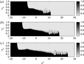
Figure 3 shows a representative full-depth simulation at various times. The computational grid employs
 $16\,384\times 512$
points, with a time step of
 $O(5\times 10^{-4})$
, although its exact size varies according to the Courant–Friedrichs–Lewy (CFL) condition. Figure 3 confirms that the buoyant current propagating to the left along the top wall is more amenable to quasi-steady modelling than the bottom current. Nevertheless, below, we will discuss comparisons between DNS simulation results and model predictions for both the upper and the lower current.
Simulation results for the density field of a full-depth, non-Boussinesq flow with
 $Re=5000$
,
 $Pe=50\,000$
and
 ${\it\sigma}=0.3$
: (a)
 $t^{\ast }=14$
, (b)
 $t^{\ast }=22$
and (c)
 $t^{\ast }=30$
.

The simulation is performed in the laboratory frame, and the results are then shifted to the reference frame moving with the current front during postprocessing. To this end, we employ linear interpolation to find the tip of the upper current as the location where
 ${\it\rho}^{\ast }=({\it\sigma}+1)/2$
along the top wall. The front velocity
 $U^{\ast }$
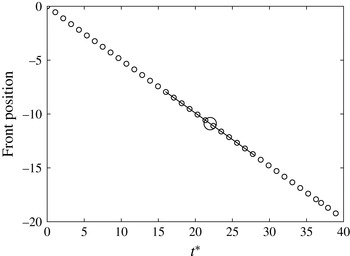
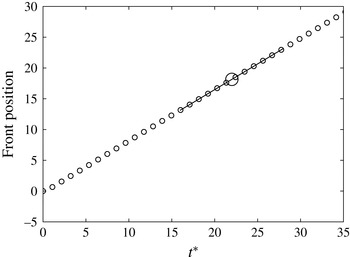
is then determined via linear regression on the front location versus time data (cf. figure 4). To shift the results to the moving reference frame,
 $U^{\ast }$
is subtracted from the laboratory-frame velocity field.
Calculation of the quasi-steady front velocity
 $U$
for the full-depth top current with
 $Re=5000$
,
 $Pe=50\,000$
and
 ${\it\sigma}=0.3$
. The small circles represent the tip location at every 2000th time step. In order to evaluate the front velocity at a given time, e.g. the large circle, we employ a local linear best fit of the front locations, as indicated by the line.

The height
 $h^{\ast }(x^{\ast },t^{\ast })$
of the top current is defined as
 $$\begin{eqnarray}h^{\ast }(x^{\ast },t^{\ast })=\frac{H}{d}-\int _{0}^{H/d}\frac{{\it\rho}^{\ast }(x^{\ast },y^{\ast },t^{\ast })-{\it\sigma}}{1-{\it\sigma}}\,\text{d}y^{\ast }.\end{eqnarray}$$
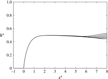
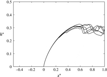
For the flow of figure 3, the current height is shown as a function of the distance behind the current tip in figure 5, at selected times. This confirms that the steady-state approximation holds with good accuracy near the front of the buoyant current.
Current height as a function of distance behind the front for a full-depth top current with
 $Re=5000$
,
 $Pe=50\,000$
and
 ${\it\sigma}=0.3$
, at
 $t^{\ast }=20$
, 22, 24, 26, 28 and 30. The steady-state approximation is seen to be valid in the vicinity of the current tip.

In order to assess the validity of Benjamin’s and the current model, we will primarily compare their predictions for the vorticity flux as a function of location with corresponding simulation results. Borden & Meiburg (Reference Borden and Meiburg2013) discuss the reasons for focusing on the vorticity flux, rather than the front velocity, primarily because of the difficulty in identifying a single representative value for the current height to use in (1.4) and (2.6). In the past, different authors have employed such measures as the first maximum in the current height behind the front, the current height at the gate location, a spatially averaged value for this purpose or the centre of mass (Anjum, McElwaine & Caulfield Reference Anjum, McElwaine and Caulfield2013). Depending on which value is selected to represent the current height, the predicted front velocities can vary appreciably, so that the front velocity is ill-suited for determining which model is more accurate.
The vorticity flux
 ${\it\Omega}_{B}$
predicted by the Benjamin model can be found by using (3.1), along with the conservation of mass,
 $$\begin{eqnarray}\frac{{\it\Omega}_{B}}{g^{\prime }d}={\it\Omega}_{B}^{\ast }=\frac{h}{d}\frac{2-{\it\alpha}}{2-2{\it\alpha}^{2}}.\end{eqnarray}$$
The corresponding vorticity flux predicted by the current model is
 $$\begin{eqnarray}\frac{{\it\Omega}_{C}}{g^{\prime }d}={\it\Omega}_{C}^{\ast }=\frac{h}{d}\end{eqnarray}$$
(cf. also equations (16) and (18) in Borden & Meiburg (Reference Borden and Meiburg2013)). Both models predict identical fluxes for
 ${\it\alpha}=1/2$
and in the limit
 ${\it\alpha}\rightarrow 0$
, i.e. for currents that either occupy half the channel height or are much smaller than the channel height. The ratio between the two predicted vorticity fluxes reaches a maximum of approximately 1.07 at
 ${\it\alpha}=2-\sqrt{3}\approx 0.268$
.
The origin of vorticity flux discrepancies between simulation results and theoretical predictions will be discussed here for the vorticity approach, with a corresponding discussion for the primitive variables approach given in appendix B. If we had kept the viscous and unsteady terms when deriving (2.3), we would have obtained
 $$\begin{eqnarray}{\it\Omega}^{\ast }={\it\Omega}_{C}^{\ast }+E_{P}^{\ast }-E_{t}^{\ast }-E_{{\it\mu}}^{\ast },\end{eqnarray}$$
where
 ${\it\Omega}^{\ast }$
represents the instantaneous dimensionless vorticity flux out of the domain. Here
 ${\it\Omega}_{C}^{\ast }$
indicates the dimensionless vorticity flux predicted by the vorticity model for the steady, inviscid case in which the gravity current fluid is at rest; and
 $E_{P}^{\ast }$
,
 $E_{t}^{\ast }$
and
 $E_{{\it\mu}}^{\ast }$
denote the deviations from this idealized model due to, respectively, fluid motion within the gravity current, unsteadiness and viscous effects,
 $$\begin{eqnarray}\displaystyle & \displaystyle E_{P}^{\ast }=\iint -\boldsymbol{{\rm\nabla}}\times \left(\frac{1}{{\it\rho}^{\ast }}\boldsymbol{{\rm\nabla}}P^{\ast }\right)\,\text{d}A^{\ast }-{\it\Omega}_{C}^{\ast }, & \displaystyle\end{eqnarray}$$
 $$\begin{eqnarray}\displaystyle & \displaystyle E_{t}^{\ast }=\iint \boldsymbol{{\rm\nabla}}\times \left(\frac{\partial \boldsymbol{u}^{\ast }}{\partial t^{\ast }}\right)\text{d}A^{\ast }, & \displaystyle\end{eqnarray}$$
 $$\begin{eqnarray}\displaystyle & \displaystyle E_{{\it\mu}}^{\ast }=-\frac{1}{Re}\iint \boldsymbol{{\rm\nabla}}\times \left(\frac{1}{{\it\rho}^{\ast }}{\rm\nabla}^{2}\boldsymbol{u}^{\ast }\right)\text{d}A^{\ast }, & \displaystyle\end{eqnarray}$$
where the integration is carried out over the control volume BCDE. The discrepancies derived in appendix B for the primitive variables approach are closely related to (3.15)–(3.17). For this reason, we will in the following section limit our discussion of the discrepancies between theoretical model predictions and simulation results to terms (3.15)–(3.17).
We furthermore remark that, if we assume a hydrostatic pressure profile along the downstream boundary B–A–E of the control volume,
 $E_{P}^{\ast }$
can alternatively be evaluated as
 $$\begin{eqnarray}E_{P}^{\ast }=(P_{O}^{\ast }-P_{B}^{\ast })\frac{{\it\sigma}-1}{{\it\sigma}}.\end{eqnarray}$$
The difference between evaluating
 $E_{P}^{\ast }$
via (3.15) and (3.18) thus provides information on how close to hydrostatic the pressure profile is along B–A–E. The pressure difference
 $P_{O}^{\ast }-P_{B}^{\ast }$
can be found by integrating the
 $x$
-momentum equation from O to B in the simulation. The
 $x$
-momentum equation yields
 $$\begin{eqnarray}\displaystyle & \displaystyle P_{O}^{\ast }-P_{B}^{\ast }=\frac{{\it\sigma}U_{B}^{\ast 2}}{2}-{\it\sigma}E_{{\it\mu},B}^{\ast }-{\it\sigma}E_{t,B}^{\ast }, & \displaystyle\end{eqnarray}$$
 $$\begin{eqnarray}\displaystyle & \displaystyle E_{{\it\mu},B}^{\ast }=\frac{1}{{\it\sigma}Re}\int _{O}^{B}{\rm\nabla}^{2}u^{\ast }\,\text{d}x^{\ast }, & \displaystyle\end{eqnarray}$$
 $$\begin{eqnarray}\displaystyle & \displaystyle E_{t,B}^{\ast }=-\int _{O}^{B}\frac{\partial u^{\ast }}{\partial t^{\ast }}\text{d}x^{\ast }. & \displaystyle\end{eqnarray}$$
Note that
 $E_{{\it\mu},B}^{\ast }$
and
 $E_{t,B}^{\ast }$
can be thought of as partial evaluations of
 $E_{{\it\mu}}^{\ast }$
and
 $E_{t}^{\ast }$
after using Stokes’ theorem. By substituting (3.19) into (3.18), one obtains
 $$\begin{eqnarray}E_{P}^{\ast }=(1-{\it\sigma})\left(-\frac{U_{B}^{\ast 2}}{2}+E_{{\it\mu},B}^{\ast }+E_{t,B}^{\ast }\right).\end{eqnarray}$$
For
 $E_{{\it\mu},B}^{\ast }\approx E_{{\it\mu}}^{\ast }$
and
 $E_{t,B}^{\ast }\approx E_{t}^{\ast }$
,
 $E_{P}^{\ast }$
,
 $E_{{\it\mu}}^{\ast }$
and
 $E_{t}^{\ast }$
will tend to cancel each other out partially in (3.14). This effect will be greatest when
 ${\it\sigma}$
and the fluid motion inside the current
 $U_{B}^{\ast }$
are both small. As
 ${\it\sigma}\rightarrow 1$
,
 $E_{P}^{\ast }\rightarrow 0$
, which is consistent with the Boussinesq vorticity model, which did not require any assumptions regarding the pressure profile inside the current.
4. Simulation results and discussion
4.1. Full-depth lock releases
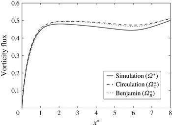
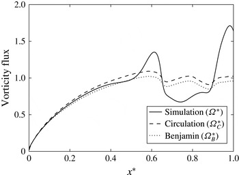
Figure 6 compares the model predictions to the vorticity flux in the simulation for the full-depth current with
 $Re=5000$
,
 $Pe=50\,000$
and
 ${\it\sigma}=0.3$
, as a function of the distance behind the current tip. We note that both model predictions are very close to the simulation result, and also to each other. This is perhaps not unexpected in light of the fact that for a full-depth current
 ${\it\alpha}\approx 0.5$
, and that for
 ${\it\alpha}=0.5$
the vorticity model (3.13) and Benjamin’s model (3.12) predict identical vorticity flux values.
Vorticity flux normalized by
 $g^{\prime }d$
versus distance
 $x^{\ast }$
behind the current head for the full-depth current with
 $Re=5000$
,
 $Pe=50\,000$
and
 ${\it\sigma}=0.3$
at
 $t^{\ast }=22$
. The values predicted by Benjamin’s model (3.12) and the circulation model (3.13) are close to each other, and to the simulation results.

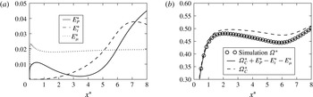
(a) Components of the difference between the vorticity flux predicted by the circulation model and the flux observed in the simulation, stemming from the three assumptions of motionless fluid inside the current (
 $E_{P}^{\ast }$
), steady state (
 $E_{t}^{\ast }$
) and inviscid flow (
 $E_{{\it\mu}}^{\ast }$
). (b) Simulation vorticity flux
 ${\it\Omega}^{\ast }$
along with
 ${\it\Omega}_{C}^{\ast }$
and
 ${\it\Omega}_{C}^{\ast }+E_{P}^{\ast }-E_{t}^{\ast }-E_{{\it\mu}}^{\ast }$
as functions of
 $x^{\ast }$
, for the full-depth current with
 $Re=5000$
,
 $Pe=50\,000$
and
 ${\it\sigma}=0.3$
at
 $t^{\ast }=22$
. All quantities are evaluated directly from the simulation data, and made dimensionless by
 $g^{\prime }d$
. The discrepancy between the vorticity flux
 ${\it\Omega}_{C}^{\ast }$
predicted by the vorticity model and the simulation result
 ${\it\Omega}^{\ast }$
is due to the quantities
 $E_{P}^{\ast }$
,
 $E_{t}^{\ast }$
and
 $E_{{\it\mu}}^{\ast }$
. Here
 $E_{P}^{\ast }$
is evaluated using (3.15).

We now analyse the magnitude of the terms that account for the deviation between the simulation result and the prediction by the vorticity model, i.e.
 $E_{P}^{\ast }$
,
 $E_{t}^{\ast }$
and
 $E_{{\it\mu}}^{\ast }$
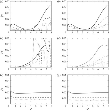
. Figure 7(a) shows the values of the integrals in (3.15)–(3.17) as functions of the distance
 $x^{\ast }$
of the control volume boundary B–A–E behind the current front. Figure 7(a) indicates that, close to the current tip, the assumption of steady flow is very accurate. Further downstream, the influence of the unsteadiness increases, which is consistent with the graphs of the current heights at various times shown in figure 5. The influence of viscous diffusion is significant near the tip of the current, but very small further downstream. The fluid motion inside the gravity current plays a significant role near the current tip, and farther downstream where the current height varies more strongly with
 $x^{\ast }$
. Figure 7(b) confirms that, if the vorticity model prediction is augmented by the three terms
 $E_{P}^{\ast }$
,
 $E_{t}^{\ast }$
and
 $E_{{\it\mu}}^{\ast }$
, the correct simulation result for the vorticity flux is recovered.
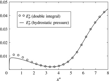
Figure 8 shows the magnitude of the pressure term
 $E_{P}^{\ast }$
as a function of the distance
 $x^{\ast }$
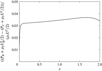
of the downstream control volume boundary B–A–E behind the current tip. The open symbols are obtained by direct integration of the integral in (3.15) from the simulation pressure field, while the solid line assumes a hydrostatic pressure profile along B–A–E and evaluates (3.18). The results are shown to be in good agreement everywhere except near the current tip, which reflects the non-hydrostatic nature of the pressure field in this region. Recall that the non-Boussinesq vorticity model made two assumptions about the pressure: (i) it assumed that the pressure distribution at the downstream boundary of the control volume is hydrostatic; and (ii) it assumed that, as a result of the current fluid being at rest,
 $P_{O}-P_{B}=0$
. Figure 8 indicates that, far behind the current front, assumption (i) is very accurate, so that assumption (ii) is largely responsible for the discrepancy between simulation results and model predictions for the vorticity flux.
Pressure-related deviation
 $E_{P}^{\ast }$
evaluated using (3.15) and (3.18), for the full-depth current with
 $Re=5000$
,
 $Pe=50\,000$
and
 ${\it\sigma}=0.3$
at
 $t^{\ast }=22$
. The difference near the tip reflects the non-hydrostatic nature of the pressure in this region, since (3.18) implied a hydrostatic pressure distribution. Farther behind the current tip, the assumption of hydrostatic pressure is very accurate. All quantities are made dimensionless by
 $g^{\prime }d$
.

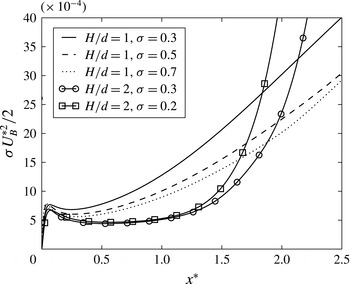
Figure 9 analyses the dependence of
 $E_{P}^{\ast }$
,
 $E_{t}^{\ast }$
and
 $E_{{\it\mu}}^{\ast }$
on the density ratio
 ${\it\sigma}$
and on
 $Re$
. We observe that increases in
 ${\it\sigma}$
or
 $Re$
tend to reduce the magnitude of all three of these terms, which indicates that predictions by the vorticity model become more accurate as the flow is less viscous and closer to Boussinesq. The decrease in
 $E_{P}^{\ast }$
for larger
 ${\it\sigma}$
is consistent with (3.22) and reflects the fact that the pressure profile inside the current becomes less influential as the flow approaches Boussinesq conditions. In order to understand the decrease in
 $E_{P}^{\ast }$
for larger
 $Re$
values, it is important to realize that for higher
 $Re$
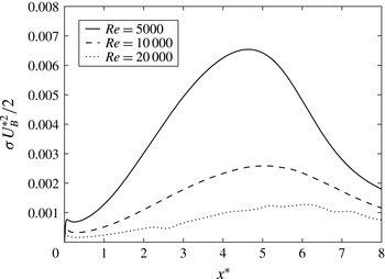
the shear layer between the current and the ambient becomes thinner, so that the ambient stream drags less current fluid with it. Consequently, the counterflow along the top wall inside the current required to replenish the loss of current fluid in the mixing layer is reduced in strength for larger
 $Re$
, which is confirmed by figure 10. Hence, the streamwise pressure gradient inside the current is weaker for higher
 $Re$
, so that
 $E_{P}^{\ast }$
is reduced.
The weaker flow inside the current for larger
 ${\it\sigma}$
and higher
 $Re$
also lowers any unsteady effects, thereby reducing
 $E_{t}^{\ast }$
. Finally, (3.20) indicates that
 $E_{{\it\mu}}^{\ast }$
scales with
 $1/({\it\sigma}Re)$
, so that it should decrease for larger values of
 ${\it\sigma}$
and
 $Re$
, which is confirmed by figure 9.
Effect of
 ${\it\sigma}$
and
 $Re$
on
 $E_{P}^{\ast }$
,
 $E_{t}^{\ast }$
and
 $E_{{\it\mu}}^{\ast }$
: (a,c,e)
 $Re=5000$
and
 ${\it\sigma}=0.3$
(solid line), 0.5 (dashed line) and 0.7 (dotted line); (b,d,f)
 ${\it\sigma}=0.3$
and
 $Re=5000$
(solid line), 10 000 (dashed line) and 20 000 (dotted line). All three of
 $E_{P}^{\ast }$
,
 $E_{t}^{\ast }$
and
 $E_{{\it\mu}}^{\ast }$
get smaller for lower viscosity and reduced density contrast, as explained in the text.

Streamwise velocity along the top wall inside the current, as a function of the distance
 $x^{\ast }$
behind the current front, for
 ${\it\sigma}=0.3$
. For increasing
 $Re$
values, the flow inside the current is reduced.

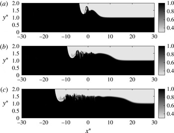
Density field of a partial-depth, non-Boussinesq gravity current with
 $Re=5000$
,
 $Pe=50\,000$
,
 ${\it\sigma}=0.3$
and
 $d/H=0.5$
: (a)
 $t^{\ast }=6$
, (b)
 $t^{\ast }=14$
and (c)
 $t^{\ast }=22$
.

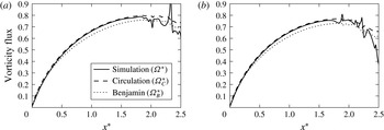
Vorticity flux versus distance behind the current tip for the partial-depth current with
 $Re=5000$
,
 $Pe=50\,000$
,
 $d/H=0.5$
and
 ${\it\sigma}=0.2$
(a) and
 ${\it\sigma}=0.3$
(b) at
 $t^{\ast }=6$
. For both density ratios, the circulation model (3.13) is seen to agree very closely with the simulation results. Benjamin’s model (3.12), while not quite as close, nevertheless also yields good quantitative agreement.

Head-loss inside the current along the top wall, for the partial-depth current with
 $Re=5000$
,
 $Pe=50\,000$
,
 $d/H=0.5$
and
 ${\it\sigma}=0.3$
at
 $t^{\ast }=6$
. The head-loss is limited to approximately 3–4 % of the free-stream kinetic energy, which explains the good quantitative agreement between Benjamin’s model predictions and the simulation results.

4.2. Partial-depth lock releases
Figure 11 shows the evolution of a partial-depth gravity current from a lock with
 $d/H=1/2$
. The front of the buoyant current is not as smooth as that of the corresponding full-depth current discussed earlier, as a result of instabilities that emerge along the interface. Nevertheless, figure 12 indicates that, for both values of
 ${\it\sigma}$
tested, the vorticity model predicts the vorticity flux accurately near the front. Benjamin’s model, while not quite as close to the DNS results as the vorticity model, nevertheless shows good quantitative agreement with the simulation data, which indicates that his zero-head-loss assumption closely approximates the situation in the simulated flow. This is confirmed by figure 13, which demonstrates that (for the present case of slip walls) the head-loss along the wall is limited to approximately 3–4 % of the free-stream kinetic energy.
The reasons for the good agreement between the vorticity model predictions and the simulation data become clear from figure 14, which shows the fluid velocity along the top wall inside the current, for several full- and half-depth currents. The partial-depth currents generally give rise to smaller velocities inside the current. This is a consequence of the weaker acceleration of the ambient fluid around the tip of partial-depth currents, so that partial-depth currents experience less shear and a lower momentum transfer. Equation (3.22) indicates that the weaker values of
 $U_{B}^{\ast }$
associated with half-depth currents enhance the partial cancellation of
 $E_{P}^{\ast }$
by
 $E_{{\it\mu}}^{\ast }$
and
 $E_{t}^{\ast }$
, thereby resulting in improved model predictions.
Fluid velocity inside the current along the top wall. Near the current tip, partial-depth currents (shown at
 $t^{\ast }=6$
) exhibit smaller velocities than full-depth currents (shown at
 $t^{\ast }=22$
).

Deviation
 $E_{P}^{\ast }$
due to the fluid motion inside the gravity current, evaluated from (3.15) (circles) and (3.18) (solid line), respectively. The simulations are the same as in figure 11 at
 $t^{\ast }=6$
with
 ${\it\sigma}=0.2$
(a) and
 ${\it\sigma}=0.3$
(b), and all quantities are made dimensionless by
 $g^{\prime }d$
.

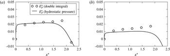
Figure 15 shows the deviation
 $E_{P}^{\ast }$
due to the fluid motion inside the gravity current, evaluated from (3.15) and (3.18), respectively. The two results agree closely with each other in the vicinity of the current tip, which demonstrates that the pressure is approximately hydrostatic there, despite the interfacial instabilities. Consistent with our earlier observations for full-depth currents, the deviation decreases for larger
 ${\it\sigma}$
. Furthermore, the values of
 $E_{P}^{\ast }$
and
 $E_{{\it\mu}}^{\ast }$
as a fraction of
 ${\it\Omega}_{C}^{\ast }$
are only about half as large as for the full-depth current. This also contributes to the good agreement observed in figure 12.
Calculation of the quasi-steady front velocity
 $U$
for the full-depth bottom current with
 $Re=5000$
,
 $Pe=50\,000$
and
 ${\it\sigma}=0.3$
. The small circles represent the tip location at every 2000th time step. In order to evaluate the front velocity at a given time, e.g. the large circle, we employ a local linear best fit of the front locations, as indicated by the line.

Current height as a function of distance behind the front for a full-depth bottom current with
 $Re=5000$
,
 $Pe=50\,000$
and
 ${\it\sigma}=0.3$
, at
 $t^{\ast }=20$
, 22, 24, 26, 28 and 30. The steady-state approximation is seen to be valid in the vicinity of the current tip, although this steady-state region is significantly shorter than that for the top current.

4.3. Dense currents
We now focus on the dense current moving towards the right along the bottom wall in figure 3. Figure 16 indicates that this current also has a steady front velocity. Figure 17 shows the bottom current heights for several times, corresponding to figure 5 for the top current. While a steady-state region again develops near the tip, it is much shorter than that for the top current, as a result of the turbulent billows. Figure 18 compares DNS results and model predictions for the vorticity flux in this region. The prediction for the vorticity flux given by the Benjamin model is
 $$\begin{eqnarray}\frac{{\it\Omega}_{B}}{g^{\prime }d}={\it\Omega}_{B}^{\ast }=\frac{h}{d}\frac{2-{\it\alpha}}{2{\it\sigma}(1-{\it\alpha}^{2})};\end{eqnarray}$$
the corresponding vorticity flux predicted by the current model is
 $$\begin{eqnarray}\frac{{\it\Omega}_{C}}{g^{\prime }d}={\it\Omega}_{C}^{\ast }=\frac{h}{d}\frac{1}{{\it\sigma}}.\end{eqnarray}$$
These predictions differ from (3.12) and (3.13) by a factor of
 $1/{\it\sigma}$
. Good agreement is seen for both models, in spite of the fact that the hydrostatic pressure assumption may not be very accurate so close to the tip.
Vorticity flux normalized by
 $g^{\prime }d$
versus distance
 $x^{\ast }$
behind the current head, for the full-depth bottom current with
 $Re=5000$
,
 $Pe=50\,000$
and
 ${\it\sigma}=0.3$
at
 $t^{\ast }=22$
. In the steady-state region near the tip, the values predicted by Benjamin’s model (4.1) and the circulation model (4.2) are close to each other, and to the simulation results.

5. Summary and conclusions
In the present investigation we have extended the vorticity-based modelling approach by Borden & Meiburg (Reference Borden and Meiburg2013) to non-Boussinesq gravity currents. This approach enables us to arrive at a closed-form solution for the Froude number without having to invoke an energy-based closure assumption, such as had been required in the analyses by von Kármán (Reference von Kármán1940) and Benjamin (Reference Benjamin1968). Hence the vorticity approach bypasses the discussion among those authors as to which energy closure provides the optimal fit with experimental and simulation data.
In the Boussinesq limit, it had been possible to decouple the pressure entirely from the conservation equations for mass and vorticity, so that no assumptions whatsoever had been required regarding the pressure. For non-Boussinesq currents, on the other hand, the pressure does not decouple from the vorticity transport equation, so that a certain amount of information regarding the pressure is needed for the exact integration of the vorticity equation over a finite control volume. To this end, we stipulate that the pressure distribution inside the current is hydrostatic. Furthermore, we assume the pressure inside the current to be constant along the wall, since the current fluid is considered to be at rest. On this basis we obtain a closed-form solution for the Froude number of non-Boussinesq gravity currents that reduces to the correct expression derived for the Boussinesq limit.
In order to assess the accuracy of the predictions by the various models for non-Boussinesq flows, we analyse the rate at which vorticity is convected out of the control volume. For full-depth currents, the prediction by the vorticity model is close to that of Benjamin’s model, and both are very close to corresponding high-resolution simulation data. For partial-depth currents, the vorticity model agrees closely with simulation data. We show that Benjamin’s model predictions also reproduce the DNS results with good accuracy, which indicates that the simulated flow satisfies Benjamin’s assumption of vanishing head-loss to a good approximation. Hence, the key contribution of the vorticity model should be seen in its ability to predict the front velocity without any energy-based closure assumptions, rather than in its improved accuracy.
We furthermore discuss the influence of the three main assumptions underlying all of the above models, including the present vorticity-based model, regarding the nature of the flow, namely that: (i) the flow is steady in the reference frame moving with the current front; (ii) the flow is inviscid; and (iii) the fluid inside the current is at rest. We find the quasi-steady flow assumption to be very accurate in the neighbourhood of the front of the top current, although unsteady effects increase farther downstream. The influence of viscosity is significant near the front, but very small further downstream. The effects of the fluid motion inside the current are small at an intermediate distance of a few current heights behind the tip, but they increase both farther downstream and in the immediate neighbourhood of the tip. For a constant density ratio, the model predictions generally improve with increasing Reynolds number; while for a constant Reynolds number, they improve for weaker density contrasts. We furthermore show that the effects of the above three assumptions partially cancel each other out with regard to the predicted vorticity flux, which explains the good agreement with simulation data across the entire range of Reynolds numbers and density ratios investigated.
Acknowledgements
This work emerged from a collaboration between E.M., S.G.L.S. and J. Rottman at the 2013 Woods Hole Summer Program on Geophysical Fluid Dynamics. E.M. and S.G.L.S. are grateful to J. Rottman and P. Linden for a number of helpful discussions during this program. E.M. acknowledges support through NSF grant CBET-1335148.
Appendix A. Extension to three-dimensional flows
The steady-state Euler equation can be written in conservative form as
 $$\begin{eqnarray}\displaystyle \boldsymbol{{\rm\nabla}}\boldsymbol{\cdot }({\it\rho}\boldsymbol{u}\boldsymbol{u})+\boldsymbol{{\rm\nabla}}p & = & \displaystyle {\it\rho}\boldsymbol{g}.\end{eqnarray}$$
We define
 $L$
as the
 $z$
component of the curl of (A 1). We take
 $y$
as the vertical direction so that
 $\boldsymbol{g}=(0,-g,0)$
, and denote the velocity components by
 $\boldsymbol{u}=(u,v,w)$
. Then we can write
 $L=\boldsymbol{{\rm\nabla}}\boldsymbol{\cdot }\boldsymbol{q}$
, where
 $$\begin{eqnarray}\boldsymbol{q}=\left(\begin{array}{@{}r@{}}q_{x}\\ q_{y}\\ q_{z}\end{array}\right)=\left(\begin{array}{@{}c@{}}g{\it\rho}+\partial _{x}(uv{\it\rho})+\partial _{z}(vw{\it\rho})+{\textstyle \frac{1}{2}}\partial _{y}[{\it\rho}(v^{2}-u^{2})]\\ -\partial _{y}(uv{\it\rho})-\partial _{z}(uw{\it\rho})+{\textstyle \frac{1}{2}}\partial _{x}[{\it\rho}(v^{2}-u^{2})]\\ 0\end{array}\right).\end{eqnarray}$$
Here
 $\boldsymbol{q}$
is arbitrary up to a gauge transformation, so that we can add the curl of any vector field to
 $\boldsymbol{q}$
and still have
 $L=\boldsymbol{{\rm\nabla}}\boldsymbol{\cdot }\boldsymbol{q}$
. We have used this choice so that
 $q_{z}=0$
.
If the system is two-dimensional or periodic in the spanwise direction, then on applying the divergence theorem there is no boundary in the
 $z$
direction, so that there will be no contribution from
 $q_{z}$
. If sidewalls are present, we need to integrate
 $q_{z}$
on the walls. However, the integral is zero, so that again there is no contribution.
Now consider
 $q_{y}$
on the basal and top surfaces where
 $v=0$
. Using the continuity equation,
 $$\begin{eqnarray}q_{y}=-u{\it\rho}\partial _{y}v-\partial _{z}(uw{\it\rho})-{\textstyle \frac{1}{2}}\partial _{x}({\it\rho}u^{2})=u{\it\rho}\partial _{z}w-\partial _{z}(uw{\it\rho})-{\textstyle \frac{1}{2}}u^{2}\partial _{x}{\it\rho}.\end{eqnarray}$$
When we integrate with respect to
 $z$
, the
 $\partial _{z}(uw{\it\rho})$
term will be zero whether the system is periodic or has sidewalls. All of these terms are likely to be small in the limit of time averaging, low diffusion and high Reynolds number. This follows for the
 $u{\it\rho}\partial _{z}w$
term in the periodic case through symmetry arguments, although in the presence of sidewalls there may be some mean contribution.
Finally, we have the
 $q_{x}$
term to consider. The
 $y$
integration of
 $\partial _{y}({\it\rho}v^{2})/2$
will be zero, since
 $v$
vanishes on the top and basal surfaces. Integration of
 $\partial _{z}(vw{\it\rho})$
in
 $z$
results in zero for both periodic boundaries and sidewalls
 $(w=0)$
. With these simplifications,
 $q_{x}$
can be written as
 $$\begin{eqnarray}q_{x}=g{\it\rho}+\partial _{x}(uv{\it\rho})-{\textstyle \frac{1}{2}}\partial _{y}({\it\rho}u^{2}).\end{eqnarray}$$
In the same manner as in § 2.2, we assume that the integration in
 $y$
and
 $z$
of
 $\partial _{x}(uv{\it\rho})$
is zero. Then
 $$\begin{eqnarray}q_{x}=g{\it\rho}-{\textstyle \frac{1}{2}}\partial _{y}({\it\rho}u^{2}),\end{eqnarray}$$
so that we recover the same result for three dimensions as we had in two dimensions.
Appendix B. Vorticity flux deviations for the primitive variables approach
An equation corresponding to (3.14) for the vorticity approach will now be derived for the primitive variables approach in two dimensions. We start with the conservative equations,
 $$\begin{eqnarray}\displaystyle & \displaystyle \partial _{t}({\it\rho}u)+\partial _{x}({\it\rho}u^{2})+\partial _{y}({\it\rho}uv)+\partial _{x}P-{\it\mu}{\rm\nabla}^{2}u=0, & \displaystyle\end{eqnarray}$$
 $$\begin{eqnarray}\displaystyle & \displaystyle \partial _{t}({\it\rho}v)+\partial _{x}({\it\rho}uv)+\partial _{y}({\it\rho}v^{2})+\partial _{y}P-{\it\mu}{\rm\nabla}^{2}v+{\it\rho}g=0. & \displaystyle\end{eqnarray}$$
Taking the
 $z$
component of the curl, dividing by
 ${\it\rho}_{1}U_{b}^{2}$
and integrating over BCDE gives
 $$\begin{eqnarray}E_{t}^{\ast }+\frac{1}{{\it\rho}_{1}U_{b}^{2}}\oint \boldsymbol{q}\boldsymbol{\cdot }\hat{\boldsymbol{n}}\,\text{d}l+\mathop{E}_{{\it\mu}}^{\ast }=0,\end{eqnarray}$$
where
 $$\begin{eqnarray}\boldsymbol{q}=\left(\begin{array}{@{}c@{}}g{\it\rho}+\partial _{x}({\it\rho}uv)+\frac{1}{2}\partial _{y}({\it\rho}(v^{2}-u^{2}))\\ -\partial _{y}({\it\rho}uv)+\frac{1}{2}\partial _{x}({\it\rho}(v^{2}-u^{2}))\end{array}\right),\end{eqnarray}$$
and
 $U_{b}=\sqrt{g(1-{\it\sigma})H}$
is the buoyancy velocity. The terms
 $E_{t}^{\ast }$
and
 $E_{{\it\mu}}^{\ast }$
are given by
 $$\begin{eqnarray}\displaystyle & \displaystyle E_{t}^{\ast }=\iint \boldsymbol{{\rm\nabla}}^{\ast }\times (\partial _{t}({\it\rho}^{\ast }\boldsymbol{u}^{\ast }))\,\text{d}A^{\ast }, & \displaystyle\end{eqnarray}$$
 $$\begin{eqnarray}\displaystyle & \displaystyle E_{{\it\mu}}^{\ast }=-\frac{1}{Re}\iint \boldsymbol{{\rm\nabla}}^{\ast }\times ({\rm\nabla}^{\ast 2}\boldsymbol{u}^{\ast })\,\text{d}A^{\ast }. & \displaystyle\end{eqnarray}$$
Integrating the second term in (B 3), and using the fact that
 $v=0$
on the top and bottom walls, as well as
 $u_{C}=u_{D}$
, gives
 $$\begin{eqnarray}\displaystyle \oint \boldsymbol{q}\boldsymbol{\cdot }\hat{\boldsymbol{n}}\,\text{d}l & = & \displaystyle \displaystyle \int _{DE+BC}\frac{1}{2}u^{2}\partial _{x}{\it\rho}\,\text{d}x+\int _{EB+CD}g{\it\rho}\,\text{d}y\nonumber\\ \displaystyle & & \displaystyle +\,\int _{EB+CD}\partial _{x}({\it\rho}uv)\,\text{d}y-\displaystyle \frac{1}{2}{\it\rho}_{B}u_{B}^{2}+\frac{1}{2}{\it\rho}_{E}u_{E}^{2}.\end{eqnarray}$$
The vorticity flux is defined as
 $$\begin{eqnarray}{\it\Omega}=\int _{EB}u(\partial _{x}v-\partial _{y}u)\,\text{d}y=\int _{EB}u\partial _{x}v\,\text{d}y-\int _{EB}\frac{1}{2}\partial _{y}(u^{2})\,\text{d}y=\int _{EB}u\partial _{x}v\,\text{d}y-\frac{1}{2}(u_{B}^{2}-u_{E}^{2}).\end{eqnarray}$$
Consequently
 $$\begin{eqnarray}\displaystyle -\frac{1}{2}{\it\rho}_{B}u_{B}^{2}+\frac{1}{2}{\it\rho}_{E}u_{E}^{2} & = & \displaystyle \displaystyle \frac{1}{2}{\it\rho}_{E}(u_{E}^{2}-u_{B}^{2})+\frac{1}{2}u_{B}^{2}({\it\rho}_{E}-{\it\rho}_{B})\nonumber\\ \displaystyle & = & \displaystyle \displaystyle {\it\rho}_{E}{\it\Omega}-{\it\rho}_{E}\int _{EB}u\partial _{x}v\,\text{d}y+\frac{1}{2}u_{B}^{2}({\it\rho}_{E}-{\it\rho}_{B}).\end{eqnarray}$$
Substituting (B 9) into (B 7) gives
 $$\begin{eqnarray}\displaystyle \oint \boldsymbol{q}\boldsymbol{\cdot }\hat{\boldsymbol{n}}\,\text{d}l & = & \displaystyle \displaystyle \int _{DE+BC}\frac{1}{2}u^{2}\partial _{x}{\it\rho}\,\text{d}x+\int _{EB+CD}g{\it\rho}\,\text{d}y+\int _{EB+CD}\partial _{x}({\it\rho}uv)\,\text{d}y\nonumber\\ \displaystyle & & \displaystyle +\displaystyle \,{\it\rho}_{E}{\it\Omega}-{\it\rho}_{E}\int _{EB}u\partial _{x}v\,\text{d}y+\frac{1}{2}u_{B}^{2}({\it\rho}_{E}-{\it\rho}_{B}).\end{eqnarray}$$
We can divide by
 ${\it\rho}_{1}U_{b}^{2}$
and substitute this back into (B 3). Since
 ${\it\rho}_{E}={\it\rho}_{1}$
for a top current,
 $$\begin{eqnarray}\displaystyle \frac{1}{{\it\rho}_{1}U_{b}^{2}}\oint \boldsymbol{q}\boldsymbol{\cdot }\hat{\boldsymbol{n}}\,\text{d}l & = & \displaystyle \displaystyle \int _{DE+BC}\frac{1}{2}u^{\ast 2}\partial _{x}{\it\rho}^{\ast }\,\text{d}x^{\ast }+\int _{EB+CD}\frac{{\it\rho}^{\ast }}{1-{\it\sigma}}\,\text{d}y^{\ast }+\int _{EB+CD}\partial _{x}({\it\rho}^{\ast }u^{\ast }v^{\ast })\,\text{d}y^{\ast }\nonumber\\ \displaystyle & & \displaystyle +\,{\it\Omega}^{\ast }-\int _{EB}u^{\ast }\partial _{x}v^{\ast }\,\text{d}y^{\ast }+\frac{1}{2}u_{B}^{\ast 2}(1-{\it\rho}_{B}^{\ast }).\end{eqnarray}$$
The second integral on the right-hand side can be evaluated piecewise,
 $$\begin{eqnarray}\int _{EB+CD}\frac{{\it\rho}^{\ast }}{1-{\it\sigma}}\,\text{d}y^{\ast }=\frac{1}{1-{\it\sigma}}((1-h^{\ast })+{\it\sigma}h^{\ast }-1)=\frac{1}{1-{\it\sigma}}(h^{\ast }({\it\sigma}-1))=-h^{\ast }=-{\it\Omega}_{C}^{\ast }.\end{eqnarray}$$
We can define the error in this piecewise evaluation such that
 $$\begin{eqnarray}\int _{EB+CD}\frac{{\it\rho}^{\ast }}{1-{\it\sigma}}\,\text{d}y^{\ast }=E_{C}^{\ast }-{\it\Omega}_{C}^{\ast }.\end{eqnarray}$$
Substituting (B 13) into (B 11) and then employing this in (B 3) gives an equation for
 ${\it\Omega}^{\ast }$
,
 $$\begin{eqnarray}\displaystyle {\it\Omega}^{\ast } & = & \displaystyle {\it\Omega}_{C}^{\ast }-E_{C}^{\ast }-E_{t}^{\ast }-E_{{\it\mu}}^{\ast }-E_{a}^{\ast }\nonumber\\ \displaystyle & & \displaystyle -\,\displaystyle \frac{1}{2}u_{B}^{\ast 2}(1-{\it\rho}_{B}^{\ast })-\int _{DE+BC}\frac{1}{2}u^{\ast 2}\partial _{x}{\it\rho}^{\ast }\,\text{d}x^{\ast }+\int _{EB}u^{\ast }\partial _{x}v^{\ast }\,\text{d}y^{\ast },\end{eqnarray}$$
where
 $$\begin{eqnarray}E_{a}^{\ast }=\int _{EB+CD}\partial _{x}({\it\rho}^{\ast }u^{\ast }v^{\ast })\,\text{d}y^{\ast }.\end{eqnarray}$$
Although (B 14) contains some terms that are very similar to those in (3.14), it is generally more complicated, so that in the main body of this work we chose to evaluate the deviations from the model using the vorticity approach.