



1. Introduction
The analysis of stability and instability of Markov models has always been an important topic. One of the main problems in this area is under what conditions the chain is stable or unstable. Stability has been investigated by many researchers; see e.g. [Reference Anderson1], [Reference Chen5], [Reference Li, Liu and Zhao16], [Reference Liu and Li20], [Reference Meyn and Tweedie26], and references therein. However, there exist a number of models that exhibit instability behavior. For example, Goodman and Massey [Reference Goodman and Massey9] presented a non-ergodic Jackson network, which will not achieve steady state as time progresses. For unstable processes, the conditions under which the model has particular transient properties have also been studied by many researchers. For instance, Morozov [Reference Morozov27] studied the instability conditions for a non-homogeneous queueing network. Choi and Kim [Reference Choi and Kim6] gave non-ergodicity criteria for denumerable continuous-time Markov processes. However, existing work was only concerned about whether the processes are transient, not involved in the classification of transient Markov chains. In fact, compared with the study of the subdivision of ergodic Markov chains, there are relatively few studies on the classification of transient Markov chains. Recently, Mao and Song [Reference Mao and Song23] presented criteria on transience for discrete-time Markov chains on a general state space, including geometric transience and algebraic transience.
Markov chains of M/G/1 type and Markov chains of GI/M/1 type, which are level-independent block-structured Markov chains, have proved very useful for characterizing the phase type queues and have many interesting and important applications in various areas. Their transition matrices are given by
 \begin{equation} \mathbb{P}_M=\left(\begin{array}{c@{\quad}c@{\quad}c@{\quad}c@{\quad}c} B_{0} & B_{1} & B_{2} & B_{3} & ... \\ C_{0} & A_{1} & A_{2} & A_{3} & ... \\ 0 & A_{0} & A_{1} & A_{2} & ... \\ 0 & 0 & A_{0} & A_{1} & ...\\ \vdots & \vdots & \vdots & \vdots & \ddots \ \end{array}\right)\end{equation}
and
 \begin{equation} \mathbb{P}_{GI}=\left(\begin{array}{c@{\quad}c@{\quad}c@{\quad}c@{\quad}c} D_{0} & \tilde{A}_{0} & 0 & 0 & ... \\ D_{1} & A_{1} & A_{0} & 0 & ... \\ D_{2} & A_{2} & A_{1} & A_{0} & ... \\ D_{3} & A_{3} & A_{2} & A_{1} & ...\\ \vdots & \vdots & \vdots & \vdots & \ddots \ \end{array}\right)\end{equation}
respectively, where  $B_{0}$ and
 $D_{0}$ are square matrices of order
 $m_{0}$,
 $A_{i}$,
 $i\geq 0$, are square matrices of order m, and
 $C_{0}$ is a matrix of order
 $m\times m_{0}$,
 $\tilde{A}_{0}$ is a matrix of order
 $m_{0}\times m$,
 $B_{i}$,
 $i\geq 1$, are matrices of order
 $m_{0}\times m$, and
 $D_{i}$,
 $i\geq 1$, are matrices of order
 $m\times m_{0}$. Let
 $\mathbb{Z}_{+}=\{0,1,2,\ldots\}$ denote the set of non-negative integers. Let
 $\mathbb{N}$ be the set of positive integers, and let
 $\mathbb{N}_k=\{1, 2, \ldots, k\}$ for
 $k\geq 1$. The state space of these block-structured Markov chains can be expressed as
 $E={\bigcup_{i=0}^{\infty}L_{i}}$, where
 $L_{0}=\{(0,j), j \in \mathbb{N}_{m_{0}}\}$ and
 $L_{i}=\{(i,j), j \in \mathbb{N}_m\}$,
 $i\geq 1$. For a state (i, j), we call i the level and j the phase.
Due to the special structures of  $\mathbb{P}_{M}$ and
 $\mathbb{P}_{GI}$, many elegant results can be obtained. Ergodicity criteria for block-structured Markov processes have been studied by many authors. For example, sufficient and necessary conditions for positive recurrence of block-structured Markov chains have been reported by Neuts [Reference Neuts28, Reference Neuts29], Asmussen [Reference Asmussen2], and Bini, Latouche, and Meini [Reference Bini, Latouche and Meini4]. Hou and Liu [Reference Hou and Liu10, Reference Liu and Hou18] studied the rate of convergence of the transition function to the stationary distributions for the chain with the transition matrix
 $\mathbb{P}_{M}$ and the chain with the transition matrix
 $\mathbb{P}_{GI}$. Mao, Tai, Zhao, and Zou [Reference Mao, Tai, Zhao and Zou24] characterized ergodic properties of Markov chains of GI/G/1 type in terms of system parameters. Truncation approximations and computing algorithm of the stationary distributions of Markov chains of M/G/1 type have recently been investigated by Liu et al. [Reference Liu and Li19, Reference Liu, Li and Masuyama21] and Masuyama [Reference Masuyama25] respectively. In addition to the study of ergodicity, some researchers have investigated transient properties for block-structured Markov chains. For example, Kijima [Reference Kijima12] studied the radius of convergence for special types of block-structured Markov chains. Latouche and Taylor [Reference Latouche and Taylor13] derived criteria for transience, recurrence, and null recurrence of continuous-time Markov chains of M/G/1 type or GI/M/1 type under appropriate drift conditions. Since the general criteria in Mao and Song [Reference Mao and Song23] are not straightforward to verify for the chains
 $\mathbb{P}_{M}$ and
 $\mathbb{P}_{GI}$, in this paper we will focus on further classification of geometric transience and algebraic transience for both chains in terms of the model parameters.
The starting point of the paper is the concept of duality. Duality on block-structured Markov chains was introduced by Ramaswami [Reference Ramaswami30], which revealed a duality relationship between Markov chains of M/G/1 type and Markov chains of GI/M/1 type. This duality relationship has been further explored in the literature (see e.g. [Reference Taylor and van Houdt32] and [Reference Zhao, Li and Alfa33]). Zhao, Li, and Alfa [Reference Zhao, Li and Alfa33] extended the duality concept to an arbitrary Markov renewal process with block-structured transition matrices, from which we know that the original Markov chain with a stochastic transition matrix is positive recurrent (or transient) if and only if its dual Markov chain is transient (or positive recurrent). Since the positive recurrence and the transience can be further classified, based on these duality relationship, it is natural to conjecture that the geometric transience and algebraic transience of  $\mathbb{P}_{M}$ (or
 $\mathbb{P}_{GI}$) correspond to geometric ergodicity and algebraic ergodicity of
 $\mathbb{P}_{GI}$ (or
 $\mathbb{P}_{M}$) with some additional conditions, respectively. We are motivated to explore this conjecture.
The main contributions in this paper include a full characterization of transience classification for Markov chains of M/G/1 type and Markov chains of GI/M/1 type. Necessary and sufficient conditions for both geometric and algebraic transience are presented in terms of the model parameters. In addition, extensions of the results to continuous-time Markov chains are also obtained. The rest of the paper consists of five sections. In Section 2 we introduce some related definitions and notations for the transience for a Markov chain, and present some basic results about geometric transience and algebraic transience, respectively. In Section 3 some spectral properties are presented for the matrix generating functions G(z) and R(z). In Sections 4 and 5 we derive the necessary and sufficient conditions for both geometric transience and algebraic transience for  $\mathbb{P}_{M}$ and
 $\mathbb{P}_{GI}$, respectively. In Section 6 we make some concluding remarks. The proofs of Proposition 1 and Theorems 2, 4, and 5 are lengthy, and hence they are put in Appendices A, B, C, and D respectively.
2. Preliminaries
Let  $\{\Phi_{n}, n\in \mathbb{Z}_{+}\}$ be an irreducible discrete-time homogeneous Markov chain on a countable state space E, with one-step transition matrix
 $\mathbb{P}=(\mathbb{P}_{ij})_{i,j\in E}$. The transition matrix
 $\mathbb{P}$ is substochastic, which is not necessarily stochastic except where noted. For any non-empty subset
 $A \subset E$, the random variables
 \begin{equation*} \tau_{A}=\inf \{n\geq 1\colon \Phi_{n}\in A\}, \quad \sigma_{A}=\inf \{n\geq 0\colon \Phi_{n}\in A\}\end{equation*}
are called the first return and the first hitting times on the set A respectively. Let
 \begin{equation*} f_{iA}(n)=\mathbb{P}\{\tau_A=n\mid \Phi_{0}=i\} \end{equation*}
be the first return probability distribution, and let
 \begin{equation*} F_{iA}=\sum_{n=1}^{\infty}f_{iA}(n)=\mathbb{P}\{\tau_A<\infty \mid \Phi_{0}=i\}\end{equation*}
be the probability of  $\Phi_{n}$ ever returning to A. Define
 \begin{equation*} F_{iA}(s)=\sum_{n=1}^{\infty} s^n f_{iA}(n) \end{equation*}
to be the exponential moment of the first return time  $\tau_{A}$.
For  $n\geq 0$, we let
 $\mathbb{P}_{iA}^{n}$ be the n-step transition probabilities of the chain, that is,
 \begin{equation*} \mathbb{P}_{iA}^{n}=\mathbb{P}\{\Phi_{n}\in A\mid \Phi_0=i\},\end{equation*}
where  $\mathbb{P}_{iA}^{0}=1_{\{A\}}(i)$ and
 $1_{\{A\}}(i)$ is the indicator function. Let
 $\mathbb{P}_{i}$ denote the conditional probability of the chain given that
 $\Phi_{0}=i$, and the corresponding conditional expectation will be denoted by
 $\mathbb{E}_{i}$. When
 $A=\{i\}$ we simply write
 $\tau_A=\tau_i$, and similarly for
 $\sigma_{A}$,
 $ f_{iA}(n)$,
 $F_{iA}$,
 $F_{iA}(s)$, and
 $\mathbb{P}_{iA}^{n}$. For any
 $n\geq 2$ and any non-empty subset
 $B \subset E$, let
 $_{B}\mathbb{P}_{iA}^{n}$ be the taboo probability of the chain, that is,
 \begin{equation*} {_{B}}\mathbb{P}_{iA}^{n}= \mathbb{P}\{\Phi_{n}\in A, \Phi_{m} \not\in B, 0< m
< n\mid \Phi_0=i\}.\end{equation*}
When  $A=\{j\}$ and
 $B=\{k\}$, we simply write
 $_{B}\mathbb{P}_{iA}^{n}= {_{k}}\mathbb{P}_{ij}^{n}$.
In the following, we present the definitions of transience and recurrence, which are taken from [Reference Mao and Song23] and [Reference Chen5], respectively.
Definition 1. Let  $\Phi_{n}$ be an irreducible Markov chain. Then
 $\Phi_{n}$ is said to be transient if
 \begin{equation} \sum_{n=0}^{\infty}\mathbb{P}^{n}_{ii}<\infty\end{equation}
for some state  $i\in E$. When
 $\Phi_{n}$ is transient, it is said to be
 $\ell$-transient for an integer
 $\ell\geq 1$ if
 \begin{equation*} \sum_{n=0}^{\infty} n^{\ell} \mathbb{P}^{n}_{ii}<\infty\end{equation*}
for some state  $i\in E$, and it is said to be geometrically transient if there exists a constant
 $s> 1$ such that
 \begin{equation} \sum_{n=0}^{\infty} s^{n}\mathbb{P}^{n}_{ii}<\infty\end{equation}
for some state  $i\in E$.
Definition 2. Let  $\Phi_{n}$ be an irreducible Markov chain. Then
 $\Phi_{n}$ is said to be recurrent if
 \begin{equation*} \sum_{n=0}^{\infty}\mathbb{P}^{n}_{ii}=\infty\end{equation*}
for some state  $i\in E$. If
 $\Phi_{n}$ is recurrent, it is said to be positive recurrent if and only if
 \begin{equation*} \mathbb{E}_i[\tau_i]<\infty\end{equation*}
for some state  $i\in E$, it is said to be
 $\ell$-ergodic for an integer
 $\ell\geq 1$ if it is aperiodic and
 \begin{equation*} \mathbb{E}_i[\tau_i^{\ell}]<\infty\end{equation*}
for some state  $i\in E$, and it is said to be geometrically ergodic if it is aperiodic and there exists a constant
 $s \in (1, \infty)$ such that
 \begin{equation} \mathbb{E}_i[s^{\tau_i}]<\infty\end{equation}
for some state  $i\in E$.
(i) If the transition matrix
 $\mathbb{P}$ is not stochastic, then the irreducible Markov chain $\Phi_n$ is always transient. It is easy to see that (3) is equivalent to $F_{ii}<1$.
-
(ii) For an irreducible Markov chain
$\Phi_{n}$, (3)–(5) hold for some state $i\in E$ if and only if each of them holds for any state $i\in E$. This statement will be verified in Proposition 2. -
(iii) Obviously, if the chain
$\Phi_{n}$ is geometrically transient (ergodic) then it must be $\ell$-transient (ergodic) for any positive integer $\ell\geq 1$. -
(iv)
$\ell$-transience and geometric transience imply the value of $\mathbb{P}_{ii}^n$ tends to zero as n tends to infinity, while $\ell$-ergodicity and geometric ergodicity imply the value of $\mathbb{P}_{ii}^n$ tends to its stationary distribution as n tends to infinity.


The modified moment of the first return time, defined by  $\mathbb{E}_i[r(\tau_A)1_{\{\tau_A<\infty\}}]$ for state i and set A, was first introduced by Mao and Song [Reference Mao and Song23] to investigate algebraic and geometric transience for Markov chains. In this following we will present equivalent conditions for (3)–(4) in terms of the modified moments of the first return time on a single state or a finite non-empty set, which play a key role in the subsequent analysis of matrix-analytical models.
Proposition 1. Suppose that the chain is irreducible. Let  $r(n)=n^{\ell}$,
 $\ell\geq 1$, or
 $r(n)=s^{n}$,
 $s \geq 1$. The following statements are equivalent.
(i) For some (then for all)
$i\in E$,
\begin{equation*} \sum_{n=0}^{\infty} r(n) \mathbb{P}_{ii}^n <\infty. \end{equation*}
-
(ii) For some (then for all)
$i\in E$, $F_{ii}<1$ and $\mathbb{E}_i[r(\tau_i)1_{\{\tau_i<\infty\}}]<\infty$. -
(iii) For some (then for all) finite non-empty set
$A\subset E$,
\begin{equation*} \max_{i\in A} \sum_{n=0}^{\infty} r(n)\mathbb{P}_{iA}^n <\infty. \end{equation*}
-
(iv) For some (then for all) finite non-empty set
$A\subset E$,
\begin{equation*} \max_{i\in A} \mathbb{E}_i[r(\tau_A)1_{\{\tau_A<\infty\}}]<\infty\quad\textit{and}\quad F_{jA}<1\quad\textit{for some $j\in A$.} \end{equation*}


Proof. See Appendix A.
Remark 2. According to Remark 1 (i) and the equivalence of assertions (ii) and (iv) of Proposition 1, the chain is transient if and only if, for some finite non-empty set  $A\subset E$,
 $F_{jA}<1$ for some
 $j\in A$. In addition, according to the equivalence of assertions (i) and (iv) of Proposition 1, the chain is geometrically transient (or
 $\ell$-transient) if and only if, for some finite non-empty set
 $A\subset E$,
 $F_{jA}<1$ for some
 $j\in A$ and
 $\max_{i\in A} \mathbb{E}_i[s^{\tau_A}1_{\{\tau_A<\infty\}}]<\infty$ (or
 $\max_{i\in A} \mathbb{E}_i[{\tau_A}^{\ell}1_{\{\tau_A<\infty\}}]<\infty$).
The following proposition verifies the argument in Remark 1 (ii) and will be used later.
Proposition 2. Suppose that the chain is irreducible and transient. Let  $r(n)=n^{\ell}$,
 $\ell\geq 1$, or
 $r(n)=s^{n}$,
 $s \geq 1$.
(i) For some finite non-empty set
$A\subset E$, $\mathbb{E}_{i}[r(\tau_{A})1_{\{\tau_A<\infty\}}]<\infty$ for any $i\in A$ if and only if $\mathbb{E}_{k}[r(\tau_{B})1_{\{\tau_B<\infty\}}]<\infty$ for any $k\in E$ and any finite non-empty set $B\subset E$.-
(ii) For some finite non-empty set
$A\subset E$, $\sum_{n=0}^{\infty} r(n) P_{iA}^n <\infty$ for any $i\in A$ if and only if $\sum_{n=0}^{\infty} r(n) \mathbb{P}_{kB}^n <\infty$ for any $k\in E$ and any finite non-empty set $B\subset E$.









Proof. The necessity of (i) and (ii) can be obtained by taking the finite set  $B=A$ directly, where
 $A\subset E$ is a fixed finite non-empty set. Now we show the sufficiency. To prove the sufficiency, we let
 $k\in E$ be a state and let
 $B\subset E$ be a finite non-empty set.
(i) Since  $\mathbb{E}_{i}[r(\tau_{A})1_{\{\tau_A<\infty\}}]<\infty$ for any
 $i\in A$ and the chain is transient, assertion (iv) of Proposition 1 holds. Then, according to the equivalence in Proposition 1, assertion (ii) of Proposition 1 holds, i.e.
 $\mathbb{E}_{j}[r(\tau_{j})1_{\{\tau_j<\infty\}}]<\infty$.
For any state  $j\in B$, since the chain is irreducible, there exists some positive integer
 $\hat{n}$ such that
 $_{j}\mathbb{P}_{jk}^{\hat{n}}>0$. For any
 $n\geq \hat{n}$, we have
 \begin{equation*}\mathbb{E}_{j}[r(\tau_{j})1_{\{\tau_j<\infty\}}] \geq \sum_{n\geq \hat{n}} r(n) \ _{j}\mathbb{P}_{jk}^{\hat{n}} f_{kj}(n-\hat{n})\geq {_{j}}\mathbb{P}_{jk}^{\hat{n}} \mathbb{E}_{k}[r(\tau_{j})1_{\{\tau_j<\infty\}}].\end{equation*}
Hence we obtain that  $\mathbb{E}_{k}[r(\tau_{j})1_{\{\tau_j<\infty\}}]<\infty$, which implies that
 \begin{equation*}\mathbb{E}_{k}[r(\tau_{B})1_{\{\tau_B<\infty\}}]<\infty. \end{equation*}
(ii) Suppose that
 \begin{equation*} \sum_{n=0}^{\infty} r(n) \mathbb{P}_{iA}^n <\infty\quad\text{for any $i \in A$.} \end{equation*}
Then it is obvious that
 \begin{equation*} \sum_{n=0}^{\infty} r(n) \mathbb{P}_{ii}^n <\infty. \end{equation*}
Since the chain is irreducible, for any state  $j\in E$ there exist some positive integers
 $n_{1}$ and
 $n_{2}$ such that
 $\mathbb{P}_{ik}^{n_{1}}>0$ and
 $P_{ji}^{n_{2}}>0$. Thus we have
 \begin{equation*}\sum_{n=0}^{\infty} r(n) \mathbb{P}_{ii}^n \geq \sum_{n=0}^{\infty} r(n)\mathbb{P}_{ii}^{n+n_{1}+n_{2}}\geq \mathbb{P}_{ik}^{n_{1}}\mathbb{P}_{ji}^{n_{2}} \sum_{n=0}^{\infty} r(n)\mathbb{P}_{kj}^{n},\end{equation*}
which implies that  $\sum_{n=0}^{\infty} r(n)\mathbb{P}_{kj}^{n}<\infty$. We then have
 \begin{equation*}\sum_{n=0}^{\infty} r(n)\mathbb{P}_{kB}^{n}=\sum_{j\in B}\sum_{n=0}^{\infty}r(n)\mathbb{P}_{kj}^{n}
< \infty.\end{equation*}
Hence the proof is finished.
Remark 3. Proposition 2 tells us that
 \begin{equation*} \mathbb{E}_{i}[r(\tau_{i})1_{\{\tau_i<\infty\}}]<\infty, \quad \text{or}\quad \sum_{n=0}^{\infty} r(n) \mathbb{P}_{ii}^n <\infty, \quad\text{for some $i\in E$} \end{equation*}
if and only if
 \begin{equation*} \mathbb{E}_{k}[r(\tau_{j})1_{\{\tau_k<\infty\}}]<\infty, \quad \text{or}\quad \sum_{n=0}^{\infty} r(n) \mathbb{P}_{kj}^n <\infty,\quad\text{for all states $k,j \in E$.} \end{equation*}
3. Spectral analysis
In this section we will show some spectral properties for Markov chains of M/G/1 type and Markov chains of GI/M/1 type whose transition matrices are given by (1) and (2) respectively. In fact, spectral properties of Markov chains of M/G/1 type and Markov chains of GI/M/1 type have been investigated in considerable detail; see e.g. [Reference Gail, Hantler and Taylor8]. Here we will present several known results and their extensions, which will be employed to analyze the transient properties later. Define
 \begin{equation*} A(z)=\sum_{k=0}^{\infty}A_{k}z^{k} \quad\text{and}\quad B(z)=\sum_{k=0}^{\infty}B_{k}z^{k}. \end{equation*}
The radii of convergence of A(z) and B(z) are defined by
 \begin{equation*} \phi_{A}=\sup\{z>0\colon A(z)<\infty\} \quad\text{and}\quad \phi_{B}=\sup\{z>0\colon B(z)<\infty\} \end{equation*}
respectively, where  $\infty$ is a matrix each of whose entries is infinite, and matrix inequalities apply component-wise. Write
 $A=A(1)=\sum_{k=0}^{\infty}A_{k}$ and
 $B=B(1)=\sum_{k=0}^{\infty}B_{k}$.
Throughout the remaining part of the paper, we make the following assumption.
Assumption 1. The matrices  $\mathbb{P}_M$,
 $\mathbb{P}_{GI}$, and A are irreducible.
Let  $\boldsymbol{\mu}^{T}$ be a positive left super-regular vector of A, i.e.
 $\boldsymbol{\mu}^{T} \geq \boldsymbol{\mu}^{T} A$ and
 $\boldsymbol{\nu}=\sum_{k=0}^{\infty}kA_{k}\boldsymbol{1}$, where
 $\boldsymbol{1}$ denotes a column vector of ones with an appropriate order according to the context. If A is stochastic, then
 $\boldsymbol{\mu}^{T}$ is the unique invariant probability vector of A, i.e.
 $\boldsymbol{\mu}^{T}=\boldsymbol{\mu}^{T} A$,
 $\boldsymbol{\mu}^{T} \boldsymbol{1} = 1$. Let
 $\chi(z)$ be the Perron–Frobenius eigenvalue of A(z) and let
 $\chi^{(n)}(z)$ be the nth-order derivative of
 $\chi(z)$. Let
 $\boldsymbol{v}^{T}(z)$ and
 $\boldsymbol{u}(z)$ denote the corresponding unique (up to the constant multiples) left and right eigenvectors respectively, which can be chosen to be strictly positive and analytic component-wise, and to satisfy that
 $\boldsymbol{v}^{T}(1)=\boldsymbol{\mu}^{T}$,
 $\boldsymbol{u}(1)=\boldsymbol{1}$.
For a chain  $\Phi_{n}$ with transition matrix
 $\mathbb{P}_M$ or
 $\mathbb{P}_{GI}$, define the first passage time on level i by
 \begin{equation*} \tau_{L_{i}}=\inf\{n\geq1\colon \Phi_{n}\in L_{i}\} \end{equation*}
for  $i\geq 0$. Define
 \begin{equation*}\tilde{f}_{(i,j), (i', j')}(n)= \mathbb{P}\{\tau_{L_{i'}}=n,\Phi_n=(i', j')\mid \Phi_0=(i, j) \},\quad n\geq 1\end{equation*}
to be the probability that starting in the state (i, j) at time 0, the chain  $\Phi_{n}$ first returns to level
 $i^{\prime}$ by hitting phase
 $j^{\prime}$, after exactly n transitions. In matrix form, we write
 $\tilde{f}_{ii'}(n)=(\tilde{f}_{(i,j), (i', j')}(n))$. Define the generating function
 \begin{equation} F_{ii^{\prime}}(s)= \sum_{n=1}^{\infty} \tilde{f}_{ii^{\prime}}(n)s^{n},\end{equation}
and let  $F_{ii^{\prime}}^{(\ell)}(s)$ be the
 $\ell$th-order derivative of
 $F_{ii^{\prime}}(s)$.
3.1. Markov chains of M/G/1 type
Note that the matrix  $F_{i+1, i}(s)$,
 $i\geq 1$, is independent of i because of the level-independent property of the transition matrix
 $\mathbb{P}_M$. Thus we define
 \begin{equation*} G(s)=F_{i+1, i}(s)\end{equation*}
for any  $i\geq 1$. For brevity we write
 $G=G(1)$ and
 $G^{(\ell)}=G^{(\ell)}(1)$ for any
 $\ell\geq 1$, where
 $G^{(\ell)}(s)$ is the
 $\ell$th-order derivative of G(s).
Let  $\rho(s)$ be the maximal eigenvalue of G(s) and let
 $\rho^{(n)}(s)$ be the nth-order derivative of
 $\rho(s)$. Define
 $\boldsymbol{\zeta}^{T}(s)$ and
 $\boldsymbol{\eta}(s)$ to be the corresponding left and right non-negative eigenvectors, respectively. Now we state the following proposition.
Proposition 3. For any  $s\in [0,\infty)$, G(s) is the minimal non-negative solution to the equation
 \begin{equation}G(s)=\sum_{v=0}^{\infty}sA_{v}G^{v}(s).\end{equation}
Moreover, the maximal eigenvalue  $\rho(s)$ of G(s) is the smallest positive root of the equation with respect to
 $z\,:\!=z(s)$:
 \begin{equation} z=s\chi(z), \quad 0
< z(s)\leq \phi_{A},\end{equation}
and the right eigenvector  $\boldsymbol{\eta}(s)$ associated with
 $\rho(s)$ can be chosen to be positive.
Proof. Here we only show that  $\boldsymbol{\eta}(s)$ is positive. For the proofs of other assertions please refer to [Reference Liu and Hou18] and [Reference Neuts29].
Post-multiplying both sides of (7) by  $\boldsymbol{\eta}(s)$ yields
 \begin{equation*}\rho(s)\boldsymbol{\eta}(s)=s\sum_{v=0}^{\infty}A_{v}[\rho(s)]^{v}\boldsymbol{\eta}(s)=sA(\rho(s))\boldsymbol{\eta}(s).\end{equation*}
Equation (8) implies that  $\chi(\rho(s))=s^{-1}\rho(s)$. Applying this to the above equation leads to
 \begin{equation*} A(\rho(s))\boldsymbol{\eta}(s)=\chi(\rho(s))\boldsymbol{\eta}(s),\end{equation*}
which shows that  $\boldsymbol{\eta}(s)$ is a Perron–Frobenius eigenvector of the irreducible matrix
 $A(\rho(s))$. Hence
 $\boldsymbol{\eta}(s)$ is positive.
The following lemma presents some spectral properties about the maximal eigenvalue  $\rho(s)$. This lemma is not new except for case (iii); please refer to [Reference Kijima12] for cases (i) and (ii).
(i) Suppose that A is stochastic and
$\boldsymbol{\mu}^{T}\boldsymbol{\nu} \leq 1$. Then $\rho(1)=1$. If $\boldsymbol{\mu}^{T}\boldsymbol{\nu} < 1$ and $\phi_{A}> 1$, then $1< \rho(s) < \phi_{A}$ for some $s>1$.-
(ii) Suppose that A is stochastic and
$\boldsymbol{\mu}^{T}\boldsymbol{\nu}>1$. Then $\rho(s)< 1$ for some $s>1$. -
(iii) Suppose that A is not stochastic. Then
$\rho(s)< 1$ for some $s>1$.


Proof. Assertions (i) and (ii) follow from Lemma 2.1 in [Reference Kijima12] and Proposition 3. Now we prove assertion (iii).
If A is not stochastic, i.e.  $A\boldsymbol{1}\leq \boldsymbol{1}$, with strict inequality for some components, then
 $\chi(1) < 1$ according to Theorem 1.6 in [Reference Seneta31]. Let
 $f_{s}(z)=s\chi(z)-z$.
If  $\chi(0)> 0$, or
 $\chi(0)= 0$ and
 $\chi^{(1)}(0+)\geq 1$, we can choose some
 $s_0 \in (1, {{{1}}/{(\chi(1))}})$ such that
 $f_{s_0}(1)<0$. When
 $\chi(0)> 0$ we have
 $f_{s_0}(0)> 0$, and therefore there exists some
 $z \in (0,1)$ such that
 $f_{s_0}(z)=0$ according to the Intermediate Value Theorem. When
 $\chi(0)= 0$ and
 $\chi^{(1)}(0+)\geq 1$ we have
 $f_{s_0}(0)= 0$ and
 $f^{\prime}_{s_0}(0)> 0$, and therefore there exists a small enough
 $z_1$ such that
 $f_{s_0}(z)> 0$ for any
 $z\in(0, z_1)$. Hence there exists a
 $z_2\in (z_1,1)$ such that
 $f_{s_0}(z_2)=0$ from the Intermediate Value Theorem. It follows from Proposition 3.1 that
 $\rho(s_0)= z_2< 1$.
If  $\chi(0)= 0$ and
 $\chi^{(1)}(0+)< 1$, we choose
 $s={{1}/{(\chi^{(1)}(0+))}}$ such that
 $f_{s}(0)= 0$ and
 $f^{\prime}_{s}(0)= 0$. Thus there exists an
 $z_{3}$, strictly greater than 0 but sufficiently close to 0, such that
 $f_{s}(z_{3})= 0$, and hence
 $0 < \rho(s)= z_3< 1$.
Now we give more details about the differentiable properties of  $\chi(z)$,
 $\boldsymbol{v}^{T}(z)$,
 $\boldsymbol{u}(z)$, and
 $\rho(s)$.
Lemma 2. Suppose that A is stochastic and  $\sum_{k=0}^{\infty}k^{n}A_{k}<\infty$ for any
 $n\geq 1$. Then we have the following.
(i) The quantities
$\chi^{(n)}(1)$, $(\boldsymbol{v}^{(n)}(1))^{T}$, and $\boldsymbol{u}^{(n)}(1)$ are finite, where $\chi^{(n)}(1)$, $(\boldsymbol{v}^{(n)}(1))^{T}$, and $\boldsymbol{u}^{(n)}(1)$ are the nth-order derivatives at $z=1$ of $\chi(z)$, $\boldsymbol{v}^{T}(z)$, and $\boldsymbol{u}(z)$, respectively.-
(ii) If
$\boldsymbol{\mu^{T}}\boldsymbol{\nu}< 1$, then $\rho^{(n)}(1)<\infty$.


Proof. Statement (i) is easily derived from Theorem A.2.3 in [Reference Neuts29]. Now we show only statement (ii). From Proposition 3 we obtain
 \begin{equation}\rho(s)=s\chi(\rho(s)).\end{equation}
Differentiating both sides of (9) n times, we obtain
 \begin{equation}\rho^{(n)}(s)=\dfrac{n\chi^{(1)}(\rho(s))\rho^{(n-1)}(s)+\sum_{j=2}^{n-1}\chi^{({\kern1.3pt}j)}(\rho(s))M_{n}({\kern1.3pt}j)+ s\chi^{(n)}(\rho(s))[\rho^{(1)}(s)]^{n}}{1-s\chi^{(1)}(\rho(s))},\end{equation}
where  $M_{n}({\kern1.3pt}j)$ is the sum of items each involving factors
 $\rho^{(k)}(s), k\in \mathbb{N}_j$.
Let  $s=1$. Since A is stochastic, from Lemma 1 (i), we have
 $\rho(1)=1$. Now we prove by induction that
 $\rho^{(n)}(1)<\infty$. This obviously holds for
 $n=1$ since
 \begin{equation*}\rho^{(1)}(1)=\dfrac{\chi^{(1)}(\rho(1))}{1-s\chi^{(1)}(\rho(1))}=\dfrac{\chi^{(1)}(1)}{1-s\chi^{(1)}(1)},\end{equation*}
and  $\chi^{(1)}(1)= \boldsymbol{\mu}^{T}\boldsymbol{\nu}< 1$. Suppose that it holds for any
 $k\in \mathbb{N}_{n-1}$. From (10) we know that
 $\rho^{(n)}(1)< \infty$ if
 $\chi^{({\kern1.3pt}j)}(1)<\infty$,
 $j=1,\ldots,n$, and
 $\boldsymbol{\mu}^{T}\boldsymbol{\nu}< 1$. Hence the result of (ii) follows from assertion (i).
3.2. Markov chains of GI/M/1 type
Now we partition the transition matrix  $\mathbb{P}_{GI}$ of GI/M/1 type in (2) as
 \begin{equation*} \mathbb{P}_{GI}=\left(\begin{array}{c@{\quad}c} D_{0} & H \\ L & P \end{array}\right)\!,\end{equation*}
where H, L, and P can be easily determined accordingly. Let  $\widehat{\mathbb{P}}(s)=\sum_{k=0}^{\infty}s^{k}P^{k}$ be the fundamental matrix for P and write
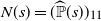 $N(s)=(\widehat{\mathbb{P}}(s))_{11}$ for the (1, 1)st block-entry in
 $\widehat{\mathbb{P}}(s)$. Let
 $\bar{\alpha}$ be the radius of convergence of P, defined by
 $\bar{\alpha}=\sup\{s>0\colon \widehat{\mathbb{P}}(s)<\infty\}$. Also, we define the (1, 1)st block-entry in
 $\widehat{\mathbb{P}}_{GI}(s)=\sum_{k=0}^{\infty}s^{k}\mathbb{P}_{GI}^{k}$ by
 $N_{0}(s)$.
Define
 \begin{equation} R(s)=s A_{0}N(s). \end{equation}
Obviously R(s) is a square matrix of size m and the (j, jʹ)th entry of R(s) can be interpreted as the total expected discounted reward with rate s induced by all visits to state  $(i+1, j^{\prime})$ before hitting any state in
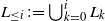 $L_{\leq i}\,:\!=\bigcup_{k=0}^{i}L_{k}$, given that the process starts in state (i, j) for any
 $i\geq 1$. It follows from (11) that R(s) satisfies the matrix equation
 \begin{equation}R(s)=\sum_{k=0}^{\infty} s R^{k}(s) A_{k}.\end{equation}
For brevity we write  $R=R(1)$ and
 $R^{(\ell)}=R^{(\ell)}(1)$ for any
 $\ell\geq 1$, where
 $R^{(\ell)}(s)$ is the
 $\ell$th-order derivative of R(s).
The censored matrix of  $\widehat{\mathbb{P}}_{GI}(s)$ to level 0 can be defined by
 \begin{equation} U_{0}(s)=s D_{0}+\sum_{k=1}^{\infty} s \tilde{A}_{0}N(s)R^{k-1}(s)s D_{k}. \end{equation}
According to the above arguments, we have
 \begin{equation} N_{0}(s)= [I-U_{0}(s)]^{-1}.\end{equation}
The matrices  $U_{0}(s)$ and
 $N_{0}(s)$ are non-negative. Let
 $u_0(s)$ and
 $n_0(s)$ denote the maximal eigenvalues of
 $U_{0}(s)$ and
 $N_{0}(s)$, respectively. For more details on the derivation and significance of the above relationships given in (12), (13), and (14), please refer to [Reference Li and Zhao14] and [Reference Li and Zhao15].
The following proposition, which establishes the duality relation of R(s) and G(s), is taken from Theorem 2.1 in [Reference Ramaswami30].
Proposition 4. Suppose that A is stochastic. Let  $\Delta$ be the diagonal matrix with
 $\boldsymbol{\mu}^T$ on the diagonal, where
 $\boldsymbol{\mu}^T$ is the invariant probability vector of A. Then
 \begin{equation} R(s)=\Delta^{-1}G^{T}(s)\Delta,\end{equation}
where G(s) is defined in (6) for  $\mathbb{P}_M$, and
 $G^{T}(s)$ is the transpose of the matrix G(s).
Remark 4. Proposition 4 leads to the following basic statements.
(i) The maximal eigenvalue of the matrix R(s) is
$\rho(s)$, where $\rho(s)$ is defined as the maximal eigenvalue of G(s).-
(ii) The left eigenvector
$\boldsymbol{\xi}^{T}(s)$ of R(s), corresponding to the maximal eigenvalue $\rho(s)$, is also a left eigenvector of $sA(\rho(s))$, which can be chosen to be positive from Proposition 3. -
(iii) The right eigenvector of R(s), corresponding to the maximal eigenvalue
$\rho(s)$, can be chosen to be $\Delta^{-1}\boldsymbol{\zeta}(s)$, where $\boldsymbol{\zeta}^{T}(s)$ is a non-negative left eigenvector of G(s) associated with the maximal eigenvalue $\rho(s)$. In particular, if the matrix G(s) is irreducible, $\boldsymbol{\zeta}^{T}(s)$ is a positive Perron–Frobenius eigenvector.


4. Transience classification for Markov chains of M/G/1 type
There exist four possible cases for the chain  $\mathbb{P}_M$.
Case 1. Both
$\mathbb{P}_{M}$ and A are stochastic.Case 2.
$\mathbb{P}_{M}$ is stochastic but A is not stochastic.Case 3.
$\mathbb{P}_{M}$ is not stochastic but A is stochastic.Case 4. Neither
$\mathbb{P}_{M}$ nor A are stochastic.


However, Case 2 cannot exist due to the special structure of  $\mathbb{P}_{M}$. In the following three theorems we will show the transience classification for Markov chains of M/G/1 type for the remaining three cases.
The matrix functions defined in Section 3 are closely related as follows; please refer to [Reference Neuts29, Chapter 2] or [Reference Liu and Hou18] for more details.
Proposition 5. For any  $s\geq 0$, we obtain
 \begin{align} F_{10}(s) &= sC_{0}+\sum_{v=1}^{\infty}sA_{v}G^{v-1}(s)F_{10}(s),\end{align}
 \begin{align} F_{00}(s) &= sB_{0}+\sum_{v=1}^{\infty}sB_{v}G^{v-1}(s)F_{10}(s).\end{align}
It was shown in [Reference Mao, Tai, Zhao and Zou24] that if  $\boldsymbol{\mu}^{T}\boldsymbol{\nu}>1$ and
 $\mathbb{P}_{GI}$ is aperiodic, then
 $\mathbb{P}_{GI}$ is geometrically ergodic. Based on the dual relation between
 $\mathbb{P}_M$ and
 $\mathbb{P}_{GI}$ on the transience and recurrence, we may conjecture that for Case 1, if
 $\boldsymbol{\mu}^{T}\boldsymbol{\nu}>1$ (equivalently,
 $\mathbb{P}_{M}$ is transient), then
 $\mathbb{P}_{M}$ is geometrically transient. The following theorem will justify this conjecture.
Theorem 1. Suppose that both  $\mathbb{P}_{M}$ and A are stochastic. If
 $\boldsymbol{\mu}^{T}\boldsymbol{\nu}>1$, then
 $\mathbb{P}_{M}$ is geometrically transient.
Proof. Let
 \begin{equation*} \tilde{G}(s)=\sum_{v=1}^{\infty}sA_{v}G^{v-1}(s). \end{equation*}
Let  $sp(\tilde{G}(s))$ be the eigenvalue of maximum modulus of
 $\tilde{G}(s)$, i.e. the spectral radius of
 $\tilde{G}(s)$. From (16) we obtain
 \begin{equation*} [I-\tilde{G}(s)]F_{10}(s)\boldsymbol{1}= sC_{0}\boldsymbol{1}.\end{equation*}
First we show that  $sp(\tilde{G}(s))< 1$ for some
 $s> 1$, which implies that
 $[I-\tilde{G}(s)]^{-1}$ exists according to Lemma 5.1.1 in [Reference Latouche and Taylor13]. From the proof of Theorem 2.3.2 in [Reference Neuts29], we know that
 $sp(\tilde{G}(1))< 1$ regardless of the value of
 $\boldsymbol{\mu}^{T}\boldsymbol{\nu}$. In addition, we have that
 $sp(\tilde{G}(s))$ is a continuous function of
 $s\in[1, s_{1}]$ for some
 $s_{1}> 1$, since
 \begin{equation} \tilde{G}(s_{1})\boldsymbol{1} \leq \sum_{v=1}^{\infty}s_{1}A_{v}G^{v-1}(s_{1})k\boldsymbol{\eta}(s_{1}) = ks_{1}\sum_{v=1}^{\infty}A_{v}\rho^{v-1}(s_{1})\boldsymbol{\eta}(s_{1})<\infty,\end{equation}
where the first inequality follows from  $k\boldsymbol{\eta}(s_{1})\geq \boldsymbol{1}$ for a bounded real number k and positive right eigenvector
 $\boldsymbol{\eta}(s_{1})$, and the last inequality follows from
 $\rho(s_{1})<1$ due to the assumption
 $\boldsymbol{\mu}^{T}\boldsymbol{\nu}>1$ and Lemma 1 (ii). Thus there exists some
 $s\in(1, s_{1}]$ such that
 $sp(\tilde{G}(s))< 1$ according to
 $sp(\tilde{G}(1))< 1$ and the continuity of the function
 $sp(\tilde{G}(s))$ on s.
Hence  $[I-\tilde{G}(s)]^{-1}$ exists and it follows that
 \begin{equation*}F_{10}(s)\boldsymbol{1}=[I-\tilde{G}(s)]^{-1}s C_{0} \boldsymbol{1}
< \infty.\end{equation*}
Therefore there exists some positive constant  $M< \infty$ such that
 $F_{10}(s)\boldsymbol{1}\leq M\boldsymbol{1}$ and
 \begin{equation} F_{00}(s)\boldsymbol{1} = sB_{0}\boldsymbol{1}+\sum_{v=1}^{\infty}sB_{v}G^{v-1}(s)F_{10}(s)\boldsymbol{1}\leq sB_{0}\boldsymbol{1}+ M\sum_{v=1}^{\infty}sB_{v}G^{v-1}(s)\boldsymbol{1}.\end{equation}
In a manner similar to the derivation of (18), we show that there exists some  $s>1$ such that
 $\sum_{v=1}^{\infty}sB_{v}G^{v-1}(s)\boldsymbol{1}<\infty$ from Lemma 1 (ii), which implies that
 $F_{00}(s)\boldsymbol{1}<\infty$ from (19). Since the chain is transient, it follows that
 $(F_{00}(1)\boldsymbol{1})_{i}<1$ for some
 $i\in \mathbb{N}_{m_{0}}$. Hence, from Remark 2 and the fact that
 \begin{equation*}(F_{00}(s)\boldsymbol{1})_{i}=\mathbb{E}_{(0, i)}[s^{\tau_{L_{0}}}1_{\{\tau_{L_{0}}<\infty\}}],\end{equation*}
we obtain that  $\mathbb{P}_{M}$ is geometrically transient.
For Case 3,  $\mathbb{P}_{M}$ is automatically transient since
 $\mathbb{P}_{M}$ is not stochastic. In this case we will present three different types of transient properties of
 $\mathbb{P}_{M}$ as follows, which vary due to the value of
 $\boldsymbol{\mu}^{T}\boldsymbol{\nu}$.
Theorem 2. Suppose that  $\mathbb{P}_{M}$ is not stochastic but A is stochastic.
(i) If
$\boldsymbol{\mu}^{T}\boldsymbol{\nu}>1$, then $\mathbb{P}_{M}$ is geometrically transient.-
(ii) If
$\boldsymbol{\mu}^{T}\boldsymbol{\nu}= 1$ and G is irreducible, then $\mathbb{P}_{M}$ is transient but not $\ell$-transient for any $\ell\geq 1$. -
(iii) If
$\boldsymbol{\mu}^{T}\boldsymbol{\nu}<1$, then $\mathbb{P}_{M}$ is geometrically transient if and only if $\min\{\phi_{A}, \phi_{B}\}> 1$, and if G is irreducible, then $\mathbb{P}_{M}$ is $\ell$-transient for some $\ell\geq 1$ if and only if $\sum_{k=0}^{\infty} k^{\ell} A_k<\infty$ and $\sum_{k=0}^{\infty} k^{\ell} B_k<\infty$.







Proof. See Appendix B.
Now we will show the transient property of  $\mathbb{P}_{M}$ for the last case.
Theorem 3. Suppose that neither  $\mathbb{P}_{M}$ nor A are stochastic. Then
 $\mathbb{P}_{M}$ is geometrically transient.
Proof. From Lemma 1 (iii) we know  $\rho(s)<1$ for some
 $s> 1$. Using the same steps as the proof of Theorem 1, we obtain that
 $F_{00}(s)\boldsymbol{1}<\infty$ for some
 $s> 1$. Since
 $\mathbb{P}_{M}$ is not stochastic, it follows that the chain is transient and
 $(F_{00}(1)\boldsymbol{1})_{i}<1$ for some
 $i\in \mathbb{N}_{m_0}$. Hence, from Remark 2 and the fact that
 \begin{equation*} (F_{00}(s)\boldsymbol{1})_{i}=\mathbb{E}_{(0, i)}[s^{\tau_{L_{0}}}1_{\{\tau_{L_{0}}<\infty\}}], \end{equation*}
we know that  $\mathbb{P}_{M}$ is geometrically transient.
5. Transience classification for Markov chains of GI/M/1 type
Similar to Markov chains of M/G/1 type, there also exist four possible cases for the chain  $\mathbb{P}_{GI}$.
Case 1ʹ. Both
$\mathbb{P}_{GI}$ and A are stochastic.Case 2ʹ.
$\mathbb{P}_{GI}$ is stochastic but A is not stochastic.Case 3ʹ.
$\mathbb{P}_{GI}$ is not stochastic but A is stochastic.Case 4ʹ. Neither
$\mathbb{P}_{GI}$ nor A are stochastic.


In fact, Theorem 4.1 in [Reference Mao, Tai, Zhao and Zou24] shows that for Case 2ʹ  $\mathbb{P}_{GI}$ is strongly ergodic, which is certainly not transient. Hence we consider the transience classification for Markov chains of GI/M/1 type only for the remaining three cases.
For Case 1ʹ,  $\mathbb{P}_{GI}$ is transient if and only if
 $\boldsymbol{\mu}^{T}\boldsymbol{\nu}<1$. It was shown in [Reference Liu and Hou18] that for Case 1 in Section 4, if
 $\boldsymbol{\mu}^{T}\boldsymbol{\nu}<1$ and
 $\mathbb{P}_M$ is aperiodic, then
 $\mathbb{P}_{M}$ is
 $\ell$-ergodic and geometrically ergodic if and only if
 $\sum_{k=1}^{\infty}k^{\ell+1} A_{k}<\infty$ and
 $\sum_{k=1}^{\infty}k^{\ell+1} B_{k}<\infty$, and
 $\min\{\phi_{A}, \phi_B\}> 1$, respectively. The dual relation between
 $\mathbb{P}_M$ and
 $\mathbb{P}_{GI}$ leads us to conjecture the criteria on
 $\ell$-transience and geometric transience for
 $\mathbb{P}_{GI}$, which are presented and confirmed as follows.
Theorem 4. Suppose that both  $\mathbb{P}_{GI}$ and A are stochastic, and
 $\boldsymbol{\mu}^{T}\boldsymbol{\nu}<1$.
(i)
$\mathbb{P}_{GI}$ is geometrically transient if and only if $\phi_{A}> 1$.-
(ii) If P and G are irreducible, then
$\mathbb{P}_{GI}$ is $\ell$-transient for some integer $\ell\geq 1$ if and only if $\sum_{k=1}^{\infty}k^{\ell+1} A_{k}<\infty$.



Proof. See Appendix C.
Remark 5. In particular, if  $\tilde{A}_{0}=A_{0}$, according to the proof of Theorem 4 (ii), the assumption that P is irreducible is redundant.
For Case 3ʹ,  $\mathbb{P}_{GI}$ is automatically transient since
 $\mathbb{P}_{GI}$ is not stochastic. Similar to M/G/1 type Markov chains, we will give three different types of transient properties for
 $\mathbb{P}_{GI}$ as follows. However, we note that the proof of these results for
 $\mathbb{P}_{GI}$ is quite different from that for
 $\mathbb{P}_M$.
Theorem 5. Suppose that  $\mathbb{P}_{GI}$ is not stochastic but A is stochastic.
(i) If
$\boldsymbol{\mu}^{T}\boldsymbol{\nu}<1$, then $\mathbb{P}_{GI}$ is geometrically transient if and only if $\phi_{A}> 1$, and $\mathbb{P}_{GI}$ is $\ell$-transient for some $\ell\geq 1$ if and only if $\sum_{k=1}^{\infty} k^{\ell+1}A_{k}<\infty$.-
(ii) If
$\boldsymbol{\mu}^{T}\boldsymbol{\nu}= 1$ and G is irreducible, then $\mathbb{P}_{GI}$ is not $\ell$-transient for any $\ell\geq 1$. -
(iii) If
$\boldsymbol{\mu}^{T}\boldsymbol{\nu}> 1$ and G is irreducible, then $\mathbb{P}_{GI}$ is geometrically transient.





Proof. See Appendix D.
Finally we will show the transient property of  $\mathbb{P}_{GI}$ for the last case.
Theorem 6. Suppose that neither  $\mathbb{P}_{GI}$ nor A are stochastic. If P is irreducible, then
 $\mathbb{P}_{GI}$ is geometrically transient.
Proof. Since A is not stochastic, from Lemma 1 (iii), it follows that  $\rho(s)< 1$ for some
 $s>1$, which implies that
 $R(s)<\infty$. According to the irreducibility of P and Proposition 2 (ii), we know that if
 $(N(s)\boldsymbol{1})_{i}<\infty$ for some
 $i\in \mathbb{N}_{m}$, then
 $(N(s)\boldsymbol{1})_{i}<\infty$ for every
 $i\in \mathbb{N}_{m}$. Thus, according to (11) and the fact that
 $A_{0}$ cannot be a zero matrix, we have
 $(N(s)\boldsymbol{1})_{i}< \infty$ for every
 $i\in \mathbb{N}_{m}$. Therefore, using the same steps as the proof in Theorem 5 (iii), we get that
 $u_{0}(s)< \infty$. Since
 $\mathbb{P}_{GI}$ is not stochastic, the chain is transient, hence
 $u_{0}(1)< 1$. Since
 $u_{0}(s)< \infty$, there exists some
 $\hat{s}> 1$ such that
 $u_{0}(\hat{s}) < 1$ and
 $n_{0}(\hat{s})<\infty$, which implies that
 $N_{0}(\hat{s})<\infty$ and
 $\mathbb{P}_{GI}$ is geometrically transient.
6. Concluding remarks
In this paper we investigate the transient properties for Markov chains of M/G/1 type and Markov chains of GI/M/1 type. Explicit criteria have been obtained for both geometric and algebraic transience. Undoubtedly it is of the same importance to investigate continuous-time Markov chains of M/G/1 type or Markov chains of GI/M/1 type, whose generators are given by (1) and (2), respectively, under appropriate modifications so that the diagonal elements are negative, the off-diagonal elements are non-negative and the sum of each row equals zero. In fact it is easy to verify that an irreducible continuous-time Markov chain with a bounded generator and its h-uniformized chain have mutually consistent transient,  $\ell$-transient, and geometrically transient classifications. Thus, by using the results in Sections 4 and 5 and the technique of uniformization (e.g. [Reference Liu17] and [Reference Liu and Hou18]), we can establish the algebraic transience and geometric transience for continuous-time Markov chains of M/G/1 type or Markov chains of GI/M/1 type.
Appendix A. Proof of Proposition 1
Proof. Since the chain is irreducible, we know that  $\sum_{n=0}^{\infty} r(n) \mathbb{P}_{ii}^n <\infty$ for some
 $i\in E$ if and only if
 $\sum_{n=0}^{\infty} r(n) \mathbb{P}_{jj}^n <\infty$ for any
 $j\in E$. Hence, to establish this result, it suffices to prove that the following statements are equivalent for any fixed
 $i\in E$ and any fixed finite set A containing i:
(iʹ)
$\sum_{n=0}^{\infty} r(n)\mathbb{P}_{ii}^n < \infty$,(iiʹ)
$F_{ii} <1, \mathbb{E}_i[r(\tau_i)1_{\{\tau_i<\infty\}}]<\infty$,(iiiʹ)
$\max_{k\in A} \sum_{n=0}^{\infty} r(n)\mathbb{P}_{kA}^n < \infty$,(ivʹ)
$F_{jA}< 1, \max_{k\in A} \mathbb{E}_k[r(\tau_A)1_{\{\tau_A<\infty\}}]<\infty$.




In the following we will establish this by showing that (iiʹ)  $\Rightarrow$ (iʹ)
 $\Rightarrow$ (iiiʹ)
 $\Rightarrow$ (ivʹ)
 $\Rightarrow$ (iiʹ).
(iiʹ)  $\Rightarrow$ (iʹ) From the first entrance decomposition of
 $\mathbb{P}_{ii}^n$, we have
 \begin{equation*} \mathbb{P}_{ii}^n = \sum_{k=1}^{n}f_{ii}(k)\mathbb{P}_{ii}^{n-k}.\end{equation*}
Thus, if  $r(n)=n^{\ell}$,
 $\ell\geq 1$, we have
 \begin{align*} \sum_{n=1}^{\infty} n^{\ell}\mathbb{P}_{ii}^n &= \sum_{n=1}^{\infty} n^{\ell}f_{ii}(n)+ \sum_{m=1}^{\infty}\mathbb{P}_{ii}^{m}\sum_{k=1}^{\infty}(m+k)^{\ell}f_{ii}(k) \notag \\* &= \sum_{n=1}^{\infty} n^{\ell}f_{ii}(n)+ \sum_{m=1}^{\infty}\mathbb{P}_{ii}^{m}\biggl[m^{\ell}\sum_{k=1}^{\infty}f_{ii}(k)+\sum_{k=1}^{\infty}k^{\ell}f_{ii}(k)+ \sum_{h=1}^{\ell-1}C_{\ell}^{h}m^{h}\sum_{k=1}^{\infty}k^{\ell-h}f_{ii}(k)\biggr]\notag \\* &\leq \mathbb{E}_i[\tau_i^{\ell}1_{\{\tau_i<\infty\}}]\biggl(1+\sum_{m=1}^{\infty}\mathbb{P}_{ii}^{m}\biggr) + F_{ii}\sum_{m=1}^{\infty}m^{\ell}\mathbb{P}_{ii}^{m}+ \mathbb{E}_i[\tau_i^{\ell}1_{\{\tau_i<\infty\}}]\sum_{h=1}^{\ell-1}C_{\ell}^{h}\sum_{m=1}^{\infty}m^{h}\mathbb{P}_{ii}^{m},\end{align*}
where  $C_{\ell}^{h}$ is the binomial coefficient and the empty sum
 $\sum_{h=1}^{0}$ is null.
Therefore we obtain
 \begin{equation} \sum_{n=1}^{\infty}n^{\ell}\mathbb{P}_{ii}^n\leq\ \dfrac{\mathbb{E}_i[\tau_i^{\ell}1_{\{\tau_i<\infty\}}]}{1-F_{ii}}\biggl[1+\sum_{m=1}^{\infty}\mathbb{P}_{ii}^{m}+ \sum_{k=1}^{\ell-1}C_{\ell}^{k}\sum_{m=1}^{\infty}m^{k}\mathbb{P}_{ii}^{m}\biggr]. \end{equation}
From (20), we use an induction argument to yield that  $\sum_{n=1}^{\infty}n^{\ell}\mathbb{P}_{ii}^n<\infty$.
If  $r(n)=s^{n}$,
 $s> 1$, since
 $F_{ii}=\sum_{n=1}^{\infty} f_{ii}(n)<1$ and
 \begin{equation*}\mathbb{E}_i[s^{\tau_i}1_{\{\tau_i<\infty\}}]=\sum_{n=1}^{\infty} s^n f_{ii}(n)<\infty,\end{equation*}
there exists some  $\hat{s}> 1$ such that
 \begin{equation*}\mathbb{E}_i[\hat{s}^{\tau_i}1_{\{\tau_i<\infty\}}]=\sum_{n=1}^{\infty} \hat{s}^n f_{ii}(n)
< 1,\end{equation*}
according to the continuity of the function  $\mathbb{E}_i[s^{\tau_i}1_{\{\tau_i<\infty\}}]$ on s. In fact, we have
 \begin{equation*} \sum_{n=0}^{\infty} \hat{s}^{n}\mathbb{P}_{ii}^n = 1 +\sum_{n=1}^{\infty}\sum_{m=1}^{n}\hat{s}^{n}f_{ii}(m)\mathbb{P}_{ii}^{n-m}=1+ \sum_{k=0}^{\infty}\hat{s}^{k}\mathbb{P}_{ii}^{k}\sum_{m=1}^{\infty}\hat{s}^{m}f_{ii}(m).\end{equation*}
Since  $\mathbb{E}_i[\hat{s}^{\tau_i}1_{\{\tau_i<\infty\}}]< 1$, we obtain that
 \begin{equation*}\sum_{n=0}^{\infty} \hat{s}^{n}\mathbb{P}_{ii}^n = \dfrac{1}{1-\mathbb{E}_i[\hat{s}^{\tau_i}1_{\{\tau_i<\infty\}}]}<\infty.\end{equation*}
In particular, when  $r(n)\equiv 1$, it is easy to show that
 \begin{equation*}\sum_{n=0}^{\infty}\mathbb{P}_{ii}^n = \dfrac{1}{1-F_{ii}}<\infty.\end{equation*}
(iʹ)  $\Rightarrow$ (iiiʹ) Assume that (iʹ) holds, that is,
 \begin{equation*}\sum_{n=0}^{\infty} r(n) \mathbb{P}_{ii}^n <\infty.\end{equation*}
Since the chain is irreducible, for any state j such that  $j\neq i$ and
 $j\in A$, there exists a positive integer
 $m>0$ such that
 $\mathbb{P}_{ji}^{m}>0$, and
 \begin{equation*} \mathbb{P}_{ji}^{m}\sum_{n=0}^{\infty}r(n)\mathbb{P}_{ij}^{n}\leq \sum_{n=0}^{\infty} r(n+m)\mathbb{P}_{ii}^{n+m}<\infty,\end{equation*}
which implies that
 \begin{equation*}\sum_{n=0}^{\infty}r(n)\mathbb{P}_{ij}^{n}<\infty.\end{equation*}
Thus, for a finite set A and any  $i\in A$, we obtain
 \begin{equation*}\sum_{n=0}^{\infty} r(n)\mathbb{P}_{iA}^n= \sum_{n=0}^{\infty}\sum_{j\in A}r(n)\mathbb{P}_{ij}^n = \sum_{n=0}^{\infty}r(n) \mathbb{P}_{ii}^n+ \sum_{j\in A, j\neq i}\sum_{n=0}^{\infty} r(n)\mathbb{P}_{ij}^n<\infty.\end{equation*}
(iiiʹ)  $\Rightarrow$ (ivʹ) Assume that (iiiʹ) holds. Obviously, for any
 $i\in A$, we have
 \begin{equation*}\mathbb{E}_i[r(\tau_A)1_{\{\tau_A<\infty\}}]=\sum_{n=0}^{\infty} r(n) F_{iA}(n)\leq \sum_{n=0}^{\infty} r(n) \mathbb{P}_{iA}^n <\infty.\end{equation*}
Now we prove that  $F_{jA}< 1$ for some
 $j\in A$. Since
 \begin{equation*} \sum_{n=0}^{\infty} r(n)\mathbb{P}_{ii}^n\leq \max_{i\in A}\sum_{n=0}^{\infty} r(n)\mathbb{P}_{iA}^n<\infty, \end{equation*}
the chain is transient. It follows from Proposition 4.21 in [Reference Chen5] that the chain is transient, i.e.  $F_{iA}<1$ for some
 $i\in E$. If
 $i\in A$, we get the assertion immediately. If
 $i \not\in A$, since the chain is irreducible, there exists some
 $j\in A$ and positive integer
 $\hat{n}$ such that
 $_{A}\mathbb{P}_{ji}^{\hat{n}}>0$. Since
 $ F_{iA}=\mathbb{P}[\tau_A<\infty\mid \Phi_{0}=i] <1$, we obtain that
 $\mathbb{P}[\tau_A=\infty \mid \Phi_{0}=i]>0$ and
 \begin{align*}&\mathbb{P}[\tau_A=\infty\mid \Phi_{0}=j] \\* &\quad \geq \mathbb{P}[\Phi_{\hat{n}+m}\not\in A, 1\leq m <\infty\mid \Phi_{0}=j, \Phi_{\hat{n}}=i, \Phi_{m} \not\in A, 1\leq m <\hat{n}] \\ &\quad\quad\, \times \mathbb{P}[\Phi_{\hat{n}}=i, \Phi_{m} \not\in A, 1\leq m <\hat{n}\mid \Phi_{0}=j] \\* &\quad = \mathbb{P}[\tau_A=\infty\mid \Phi_{0}=i]\cdot {_{A}\mathbb{P}}_{ji}^{\hat{n}} > 0,\end{align*}
which implies that  $F_{jA}=\mathbb{P}[\tau_A<\infty\mid \Phi_{0}=j] <1$.
(ivʹ)  $\Rightarrow$ (iiʹ) It is obvious that
 $F_{jj}\leq F_{jA}< 1$ for some
 $j\in A$, which implies that
 $F_{ii}< 1$ for any
 $i\in E$ according to the irreducibility of the chain. Since
 \begin{equation*}\max_{i\in A} \mathbb{E}_i[r(\tau_A)1_{\{\tau_A<\infty\}}]<\infty,\end{equation*}
from Lemma 3.3 in [Reference Liu, Zhang and Zhao22], there exists a subset  $A'\subset A$ such that
 \begin{equation*}\max_{i\in A} \mathbb{E}_i[r(\tau_{A'})1_{\{\tau_{A'}<\infty\}}]<\infty.\end{equation*}
By irreducibility, in a manner similar to Remark (2) in [Reference Anderson1, page 210], we have
 \begin{equation*}\max_{i\in A} \mathbb{E}_i[r(\tau_j)1_{\{\tau_j<\infty\}}]<\infty\quad\text{for any $j\in A$.}\end{equation*}
Then, from Remark 2.2 in [Reference Hou, Liu and Zhang11], we obtain that
 \begin{equation*}\mathbb{E}_i[r(\tau_i)1_{\{\tau_i<\infty\}}]<\infty \quad\text{for any \textit{i}.}\end{equation*}
Hence we finish the proof.
Appendix B. Proof of Theorem 2
Proof. The proof of (i) uses the same steps as the proof in Theorem 1, which is hence omitted. We only need to prove (ii) and (iii).
Differentiating both sides of (7)  $\ell$ times and taking
 $s=1$, we have
 \begin{equation} G^{(\ell)}\boldsymbol{1}= \sum_{v=1}^{\infty}A_{v}\sum_{k=0}^{v-1}G^{k}G^{(\ell)}G^{v-k-1}\boldsymbol{1}+ C_{1}\boldsymbol{1},\end{equation}
where  $C_{1}$ is a sum of items each involving the moment matrices
 $G^{(k)}$ for any k,
 $0\leq k\leq \ell-1$. When
 $\ell=1$, it is easy to obtain that
 $C_{1}=\sum_{v=0}^{\infty}A_{v}G^{v}$.
From [Reference Neuts29, page 89], we know that if A is irreducible, then G is stochastic if and only if  $\boldsymbol{\mu}^{T}\boldsymbol{\nu}\leq1$. Thus, for (ii) and (iii), (21) can be written as
 \begin{equation}[I-H ] G^{(\ell)}\boldsymbol{1}=C_{1}\boldsymbol{1},\end{equation}
where
 \begin{equation*}H=\sum_{v=1}^{\infty}A_{v}\sum_{k=0}^{v-1}G^{k}\end{equation*}
is a non-negative matrix. It is obvious that  $C_{1}\boldsymbol{1}=\boldsymbol{1}$ when
 $\ell=1$.
(ii) The proof is by contradiction: we assume that  $\mathbb{P}_{M}$ is 1-transient, which means
 \begin{equation} (F^{(1)}_{00}(1)\boldsymbol{1})_{i}=\biggl(\sum_{n=1}^{\infty}n \tilde{f}_{00}(n)\boldsymbol{1}\biggr)_{i}=\mathbb{E}_{(0, i)}[\tau_{L_{0}}1_{\{\tau_{L_{0}}<\infty\}}]<\infty\end{equation}
for any  $i\in \mathbb{N}_{m_{0}}$.
Since  $\mathbb{P}_{M}$ is irreducible, it follows from (23) and Proposition 2 (i) that for any
 $i>1$,
 \begin{equation*}1 \leq (G^{(1)}\boldsymbol{1})_{i}=\biggl(\sum_{m=1}^{\infty}m\tilde{f}_{2 1}(m)\boldsymbol{1}\biggr)_{i}=\mathbb{E}_{(2, i)}[\tau_{L_{1}}1_{\{\tau_{L_{1}}<\infty\}}]<\infty.\end{equation*}
Therefore we derive  $HG^{(1)}\boldsymbol{1}\leq G^{(1)}\boldsymbol{1}<\infty$ from (22). Since
 $G^{(1)}\boldsymbol{1}$,
 $HG^{(1)}\boldsymbol{1}$ and H are non-negative, from Lemma* in [Reference Debreu and Herstein7], we have
 $sp(H)\leq 1$, where sp(H) is the spectral radius of H. Furthermore, since G is irreducible and
 $\boldsymbol{\mu}^{T}\boldsymbol{\nu}=1$, we have that
 $I-H$ is singular from the proof of Theorem 3.1.1 in [Reference Neuts29], which implies that
 $sp(H)= 1$. Then, according to Theorem I* in [Reference Debreu and Herstein7], we obtain that there exists a non-zero left eigenvector
 $\boldsymbol{x}^{T}$ of H associated with eigenvalue 1 satisfying
 $\boldsymbol{x}^{T}\geq \boldsymbol{0}^{T}$ and
 \begin{equation*} \boldsymbol{x}^{T}(I-H)=\boldsymbol{0}^{T}.\end{equation*}
However, when  $\ell=1$, premultiplying both sides of (22) by
 $\boldsymbol{x}^{T}$ leads to a conflict that
 \begin{equation*}0=\boldsymbol{x}^{T}[I-H ] G^{(\ell)}\boldsymbol{1}=\boldsymbol{x}^{T}\boldsymbol{1} \neq 0.\end{equation*}
Hence our assumption does not hold, which means that for any  $i\in \mathbb{N}_{m_{0}}$,
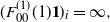 $(F^{(1)}_{00}(1)\boldsymbol{1})_{i} =\infty, $ and hence, for any
 $\ell\geq 1$,
 \begin{equation*} \biggl(\sum_{n=1}^{\infty}n^{\ell} \tilde{f}_{00}(n)\boldsymbol{1}\biggr)_{i}=\infty. \end{equation*}
Thus we get assertion (ii).
(iii) We begin with the proof of the geometric transience case.
If  $\boldsymbol{\mu}^{T}\boldsymbol{\nu}<1$ and
 $\min\{\phi_{B}, \phi_{A}\}> 1$, it follows from Lemma 1 (i) that
 \begin{equation*}1< \rho(s)
< \phi_{A}\end{equation*}
for some  $s>1$. Therefore we have that inequality (18) still holds since
 $\rho(s)< \phi_{A}$ and then, using the same steps as the proof in Theorem 1, we get that
 $\mathbb{P}_{M}$ is geometrically transient.
Conversely, if the chain is geometrically transient and  $\boldsymbol{\mu}^{T}\boldsymbol{\nu}<1$, then
 \begin{equation}F_{00}(s)\boldsymbol{1}=sB_{0}\boldsymbol{1}+\sum_{v=1}^{\infty}sB_{v}G^{v-1}(s)F_{10}(s)\boldsymbol{1} <\infty\end{equation}
for some  $s>1$, and
 $G\boldsymbol{1}=\boldsymbol{1}$, which implies that
 $F_{10}(1)\boldsymbol{1}=\boldsymbol{1}$ according to Lemma 2.4.1 in [Reference Neuts29]. Furthermore, it follows from
 $F_{00}(s)\boldsymbol{1}<\infty$ and Proposition 2 (i) that
 $G(s)<\infty$ and
 \begin{equation} F_{10}(s) \boldsymbol{1}=sC_{0}\boldsymbol{1}+\sum_{v=1}^{\infty}sA_{v}G^{v-1}(s)F_{10}(s)\boldsymbol{1}<\infty.\end{equation}
Thus we have  $F_{10}(s)\boldsymbol{1}> \boldsymbol{1}$ and
 $G(s)\boldsymbol{1}> \boldsymbol{1}$ for some
 $s>1$ due to the above arguments and the fact that
 \begin{equation*} G^{(1)}\boldsymbol{1}=\sum_{n=1}^{\infty}n\tilde{f}_{2,1}(n)\boldsymbol{1}\geq G\boldsymbol{1}=\boldsymbol{1}>\boldsymbol{0} \end{equation*}
and
 \begin{equation*} F_{10}^{(1)}(1) \boldsymbol{1}=\sum_{n=1}^{\infty}n\tilde{f}_{10}(n)\boldsymbol{1}\geq F_{10}(1) \boldsymbol{1}> \boldsymbol{0}. \end{equation*}
Hence it follows from (24), (25) and  $F_{10}(s)\boldsymbol{1}> \boldsymbol{1}$ that
 \begin{equation*} \sum_{v=1}^{\infty}sB_{v}G^{v-1}(s) <\infty\quad\text{and}\quad \sum_{v=1}^{\infty}sA_{v}G^{v-1}(s) <\infty. \end{equation*}
Post-multiplying both sides of the above inequalities by the positive vector  $\boldsymbol{\eta}(s)$, we obtain
 \begin{equation} \sum_{v=1}^{\infty}sB_{v}\rho^{v-1}(s)\boldsymbol{\eta}(s)<\infty \quad \text{and} \quad \sum_{v=1}^{\infty}sA_{v}\rho^{v-1}(s)\boldsymbol{\eta}(s)<\infty.\end{equation}
Since  $\boldsymbol{1} < G(s)\boldsymbol{1} <\infty$, from Lemma* in [Reference Debreu and Herstein7], we have
 $\rho(s)> 1$ for some
 $s>1$. Hence, from (26), we know that
 $\phi_{A}> 1$,
 $\phi_{B}> 1$ and the proof of the first statement of (iii) is finished.
Now we prove the algebraic case. Since  $\boldsymbol{\mu}^{T}\boldsymbol{\nu}< 1$, we know that
 $(I-H)^{-1}$ exists according to Theorem 3.1.1 in [Reference Neuts29]. It then follows from (22) that
 \begin{equation*}G^{(\ell)}\boldsymbol{1}=[I-H]^{-1}C_{1}\boldsymbol{1}.\end{equation*}
From the last paragraph in Section 3.1 of [Reference Neuts29], we know that  $C_{1}\boldsymbol{1}<\infty$ if and only if
 $\sum_{v=0}^{\infty}v^{\ell}A_{v}<\infty$, which implies that
 $G^{(\ell)}\boldsymbol{1}<\infty$ if and only if
 $\sum_{v=0}^{\infty}v^{\ell}A_{v}<\infty$.
Differentiating both sides of (16)  $\ell$ times and taking
 $s=1$, we have
 \begin{align*} \biggl[I-\sum_{v=1}^{\infty} A_{v}G^{v-1}\biggr] F_{10}^{(\ell)}(1)\boldsymbol{1} &= \sum_{v=2}^{\infty}A_{v}\sum_{k=0}^{v-2} G^{k}G^{(\ell)}G^{v-k-2}F_{10}(1)\boldsymbol{1}+C_{2}\boldsymbol{1} \\* &= \sum_{v=2}^{\infty}A_{v}\sum_{k=0}^{v-2} G^{k}G^{(\ell)}\boldsymbol{1}+C_{2}\boldsymbol{1}, \end{align*}
where  $C_{2}$ is a sum of items each involving the moment matrices
 $F_{10}^{(k)}(1)$ and
 $G^{(k)}$,
 $ 0\leq k\leq \ell-1$. From the proof of Theorem 3.1 in [Reference Liu and Hou18], we obtain that
 $C_{2}\boldsymbol{1}<\infty$ if and only if
 $\sum_{v=0}^{\infty}v^{\ell}A_{v}<\infty$.
In addition, if  $G^{(\ell)}\boldsymbol{1}<\infty$, we obtain
 \begin{equation*} \sum_{v=2}^{\infty} A_{v}\sum_{k=0}^{v-2} G^{k}G^{(\ell)}\boldsymbol{1} \leq \sum_{v=2}^{\infty} A_{v}\sum_{k=0}^{v-2}G^{k} h\boldsymbol{1} = h\sum_{v=2}^{\infty}(v-1) A_{v}\boldsymbol{1},\end{equation*}
where h is a bounded real number such that  $G^{(\ell)}\boldsymbol{1}\leq h\boldsymbol{1}$. Thus, since
 \begin{equation*}\biggl[I-\sum_{v=1}^{\infty} A_{v}G^{v-1}\biggr]^{-1}\end{equation*}
exists according to the proof of Lemma 2.4.1 in [Reference Neuts29], we have  $F_{10}^{(\ell)}(1)\boldsymbol{1}<\infty$ if and only if
 \begin{equation*}\sum_{v=0}^{\infty}v^{\ell}A_{v}<\infty.\end{equation*}
Similarly, differentiating both sides of (17)  $\ell$ times and taking
 $s=1$, we obtain that
 \begin{equation*}F_{00}^{(\ell)}(1)\boldsymbol{1} = \sum_{v=1}^{\infty}B_{v}G^{v-1}F_{10}^{(\ell)}(1)\boldsymbol{1}+\sum_{v=2}^{\infty}B_{v}\sum_{k=0}^{v-2} G^{k}G^{(\ell)}\boldsymbol{1}+C_{3}\boldsymbol{1},\end{equation*}
where  $C_{3}$ is a sum of items each involving the moment matrices
 $F_{10}^{(k)}(1)$ and
 $G^{(k)}$,
 $0\leq k\leq \ell-1$. According to the proof of Theorem 3.1 in [Reference Liu and Hou18] again, we get
 $F_{00}^{(\ell)}(1)\boldsymbol{1}<\infty$ if and only if
 \begin{equation*}\sum_{v=0}^{\infty}v^{\ell}A_{v}<\infty\quad\text{and}\quad\sum_{v=0}^{\infty}v^{\ell}B_{v}<\infty.\end{equation*}
Furthermore, from (6), we have
 \begin{equation} F_{00}^{(\ell)}(s)\boldsymbol{1}=\sum_{n=\ell}^{\infty} n(n-1)\cdots (n-\ell+1)s^{n-\ell} \tilde{f}_{00}(n)\boldsymbol{1}.\end{equation}
It is obvious that
 \begin{equation}\lim_{n\rightarrow\infty}\dfrac{n^{\ell}}{n(n-1)\cdots (n-\ell+1)}=1.\end{equation}
Hence from (27) and (28) we have  $F_{00}^{(\ell)}(1)\boldsymbol{1}<\infty$ if and only if
 \begin{equation*}\sum_{n=1}^{\infty}n^{\ell} \tilde{f}_{00}(n)\boldsymbol{1}<\infty.\end{equation*}
Finally, since the chain is transient, i.e.  $(F_{00}(1)\boldsymbol{1})_{i}<1$ for some
 $i\in \mathbb{N}_{m_{0}}$ according to Proposition 1, from the above arguments and Remark 2, and the fact that
 \begin{equation*}\biggl(\sum_{n=1}^{\infty}n^{\ell} \tilde{f}_{00}(n)\boldsymbol{1}\biggr)_{i}=\mathbb{E}_{(0, i)}[\tau_{L_{0}}^{\ell}1_{\{\tau_{L_{0}}<\infty\}}],\end{equation*}
we obtain the chain is  $\ell$-transient if and only if
 \begin{equation*}\sum_{k=0}^{\infty} k^{\ell} A_k<\infty\quad\text{and}\quad\sum_{k=0}^{\infty} k^{\ell} B_k<\infty.\end{equation*}
Hence we finish the proof.
Appendix C. Proof of Theorem 4
Proof. (i) If  $\phi_{A}> 1$, for any
 $z\in(0, \phi_{A})$, we have that
 $\chi(z)$ is a finite continuous function of z and the corresponding Perron–Frobenius right eigenvector
 $\boldsymbol{u}(z)$ is finite. Here we choose
 $\boldsymbol{u}(z)$ to be larger than
 $\boldsymbol{1}$ since it can be strictly positive. Let
 $\boldsymbol{W}$ be a column vector whose ith block is equal to
 $\boldsymbol{W}_{i}$, where
 $\boldsymbol{W}_{i}=({{1}/{{z}}})^{i}\boldsymbol{u}(z)$ for any
 $i\geq 1$ and any
 $z\in[1, \phi_{A})$, and
 $\boldsymbol{W}_{0}=\boldsymbol{1}$. Thus we obtain that, for
 $i\geq 1$,
 \begin{align}(\mathbb{P}_{GI}\boldsymbol{W})_i &= D_{i}\boldsymbol{1} +\sum_{k=0}^{i}A_{k}z^{k-i-1}\boldsymbol{u}(z) \notag \\* &= \sum_{k=i+1}^{\infty}A_{k} \boldsymbol{1} + \biggl(\sum_{k=0}^{\infty}A_{k}z^{k-i-1}-\sum_{k=i+1}^{\infty}A_{k}z^{k-i-1}\biggr)\boldsymbol{u}(z) \notag \\ &\leq \sum_{k=i+1}^{\infty}(1-z^{k-i-1})A_{k}\boldsymbol{u}(z)+ \sum_{k=0}^{\infty}A_{k}z^{k-i-1}\boldsymbol{u}(z)\notag \\ &\leq \sum_{k=0}^{\infty}A_{k}z^{k-i-1}\boldsymbol{u}(z) \notag \\ &= \biggl(\dfrac{1}{z}\biggr)^{i+1} \chi(z)\boldsymbol{u}(z)\notag\\* &= \dfrac{\chi(z)}{z}\boldsymbol{W}_{i}\notag \\* &<\infty,\end{align}
where the fifth equality follows from the definitions of  $\chi(z)$ and
 $\boldsymbol{u}(z)$.
Let  $\lambda(z)={{\chi(z)}/{z}}$; we have
 $\lambda(1)=1$,
 $\lambda'(1)=\chi'(1)-1=\boldsymbol{\mu}^{T}\boldsymbol{\nu}-1< 0$ and
 $\lambda(z)$ is a continuous function on
 $z\in(0, \phi_{A}]$ due to the continuity of
 $\chi(z)$. Thus we obtain that there exists some
 $\hat{z}\in (1, \phi_{A})$ such that
 $\lambda\,:\!=\lambda(\hat{z})< 1$. Since the above drift condition (29) holds, according to the proof of Case 1 of Theorem 2.6 in [Reference Chen5], we know that for any
 $i\geq 1$,
 $F_{i0}({{1}/{\lambda}})\boldsymbol{1}<\infty.$ From equation (2.5) in [Reference Mao and Song23], we have
 \begin{equation} F_{00}(s)\boldsymbol{1}=sD_{0}\boldsymbol{1}+s\tilde{A}_{0}F_{10}(s)\boldsymbol{1}, \quad s\geq 0,\end{equation}
which implies that  $F_{00}({{1}/{\lambda}})\boldsymbol{1} <\infty$. Since the chain is transient, it follows that
 $(F_{00}(1)\boldsymbol{1})_{i}<1$ for some
 $i\in \mathbb{N}_{m_{0}}$. Hence, from Remark 2 and the fact that
 \begin{equation*}(F_{00}(s)\boldsymbol{1})_{i}=\mathbb{E}_{(0, i)}[s^{\tau_{L_{0}}}1_{\{\tau_{L_{0}}<\infty\}}],\end{equation*}
we know that  $\mathbb{P}_{GI}$ is geometrically transient.
To see the converse, suppose that  $\mathbb{P}_{GI}$ is geometrically transient. Then
 $\widehat{\mathbb{P}}(s_{1})<\infty$ for some
 $s_{1}> 1$, which implies that
 $N(s_{1})<\infty$. It follows from (11) that
 $R(s_{1})<\infty$, which implies that the eigenvalue
 $\rho(s)$ is a finite continuous function of
 $s\in[1, s_{1})$. Since
 $\boldsymbol{\mu}^{T}\boldsymbol{\nu}< 1$ and A is stochastic, according to Lemma 1 (i) and (10), we have
 $\rho(1)= 1$ and
 $\rho^{(1)}(1-) > 0$. Thus, for any
 $s \in (1, s_{1})$,
 $1< \rho(s)<\infty$. From (12), we have
 \begin{equation} \rho(s)\boldsymbol{\xi}^{T}(s)= \boldsymbol{\xi}^{T}(s)R(s)=\sum_{k=0}^{\infty}\boldsymbol{\xi}^{T}(s)R^{k}(s)s A_{k}=\sum_{k=0}^{\infty}\rho^{k}(s)\boldsymbol{\xi}^{T}(s)sA_{k},\end{equation}
where  $\boldsymbol{0}<\boldsymbol{\xi}^{T}(s)<\infty$ according to Remark 4 (ii). Since the left-hand side of (31) is finite, we obtain that
 $\sum_{k=0}^{\infty}\rho^{k}(s)A_{k}<\infty$ for any
 $s \in (1, s_{1})$, which implies that
 $\phi_{A}> 1$. Hence we get assertion (i).
(ii) Now we consider the sufficiency of (ii). Suppose that  $\sum_{m=1}^{\infty}A_{m}m^{\ell+1}<\infty$. From (2) and Corollary 2.8 in [Reference Mao and Song23], we obtain that
 \begin{equation*}F_{i0}(s)\boldsymbol{1}=sD_{i}\boldsymbol{1}+sA_{i}F_{10}(s)\boldsymbol{1}+sA_{i-1}F_{20}(s)\boldsymbol{1}+\cdots +sA_{0}F_{i+1, 0}(s)\boldsymbol{1},\quad i\geq1.\end{equation*}
Define
 \begin{equation*}F(s,z)=\sum_{i=1}^{\infty}z^{i}F_{i0}(s)\boldsymbol{1}\quad \text{and} \quad D(z)= \sum_{k=1}^{\infty}z^{k}D_{k}\boldsymbol{1},\quad s< 1,\ z<1.\end{equation*}
Then we have
 \begin{align} F(s,z)&= sA(z)F_{10}(s)\boldsymbol{1}+\cdots+sz^{i-1}A(z)F_{i0}(s)\boldsymbol{1}+\cdots+sD(z)\boldsymbol{1}-sA_{0}F_{10}(s)\boldsymbol{1}\notag \\* &= \dfrac{sA(z)[F(s,z)]}{z} +sD(z)\boldsymbol{1}-sA_{0}F_{10}(s)\boldsymbol{1}.\end{align}
From (32) we get that
 \begin{equation*} (zI-sA(z))F(s,z)=sz[D(z)-A_{0}F_{10}(s)]\boldsymbol{1},\quad s<1,\ z<1.\end{equation*}
According to the definitions of  $\chi(z)$ and
 $\boldsymbol{v}^{T}(z)$, we have
 \begin{equation} \boldsymbol{v}^{T}(z)(zI-sA(z))= \boldsymbol{v}^{T}(z)(z-s\chi(z)). \end{equation}
From Proposition 3, we know that  $z=\rho(s)< 1$,
 $s< 1$ is a zero point of the right-hand side of (33), which implies that
 $z=\rho(s)$ is also a zero point of the equation
 $\boldsymbol{v}^{T}(z)(zI-sA(z))=0$. According to the definition of F(s, z), we know that F(s, z) is analytic on
 $s<1$ and
 $z<1$. Thus
 $z=\rho(s)$ is also a zero point of
 $\boldsymbol{v}^{T}(z) [D(z)-A_{0}F_{10}(s)]$, that is,
 \begin{equation} \boldsymbol{v}^{T}(\rho(s)) D(\rho(s))\boldsymbol{1}= \boldsymbol{v}^{T}(\rho(s))A_{0}F_{10}(s)\boldsymbol{1}.\end{equation}
Since  $\rho(s)$ and
 $\boldsymbol{v}^{T}(\rho(s))$ are continuous functions of s, we deduce from Lemma 1 (i) that
 $\rho(1)=1$ and
 $ \boldsymbol{v}^{T}(\rho(1))=\boldsymbol{\mu}^{T}$, where
 $\boldsymbol{\mu}^{T}$ is the invariant probability vector of A. Differentiating both sides of (34)
 $\ell$ times and taking
 $s=1$, we have
 \begin{align}&\sum_{k=1}^{\ell}c_{0k}(\boldsymbol{v}^{(k)}(1))^{T}A_{0}F_{10}(1)\boldsymbol{1}+ \sum_{k=1}^{\ell-1}c_{1k}(\boldsymbol{v}^{(k)}(1))^{T}A_{0}F_{10}^{(1)}(1)\boldsymbol{1}+\cdots+ \boldsymbol{\mu}^{T} A_{0}F^{(\ell)}_{10}(1)\boldsymbol{1}\notag \\* &\quad = \sum_{k=1}^{\ell}d_{0k}(\boldsymbol{v}^{(k)}(1))^{T}D(1)\boldsymbol{1}+ \sum_{k=0}^{\ell-1}d_{1k}(\boldsymbol{v}^{(k)}(1))^{T}D^{(1)}(1)\boldsymbol{1}+\cdots+ \boldsymbol{\mu}^{T} D^{(\ell)}(1)\boldsymbol{1},\end{align}
where  $c_{0k}, \ldots, c_{\ell-1,k}, d_{0k}, \ldots, d_{{\ell-1,k}}$, are bounded factors from Lemma 2 (ii).
For  $\ell=1$, according to (35), we have
 $\boldsymbol{\mu}^{T} A_{0}F_{10}^{(1)}(1)\boldsymbol{1}<\infty$ if and only if
 $\boldsymbol{\mu}^{T} D^{(1)}(1)\boldsymbol{1}<\infty$. Similarly, for
 $\ell=2$, we also get
 $\boldsymbol{\mu}^{T} A_{0}F_{10}^{(2)}(1)\boldsymbol{1}<\infty$ if and only if
 $\boldsymbol{\mu}^{T} D^{(2)}(1)\boldsymbol{1}<\infty$. The rest can be deduced by using an inductive argument. Hence we obtain that
 $\boldsymbol{\mu}^{T} A_{0}F_{10}^{(\ell)}(1)\boldsymbol{1}<\infty$ if and only if
 $\boldsymbol{\mu}^{T} D^{(\ell)}(1)\boldsymbol{1}<\infty$ for any
 $\ell\geq 1$.
From the definition of D(z), we obtain that
 \begin{align*}D^{(\ell)}(1)\boldsymbol{1} &= \sum_{k=\ell}^{\infty} k(k-1)\cdots(k-\ell+1)D_{k}\boldsymbol{1}\\* &= \sum_{m=\ell+1}^{\infty} A_{m}\boldsymbol{1} \sum_{k=\ell}^{m-1} k(k-1)\cdots(k-\ell+1)\\* &\leq \sum_{m=2}^{\infty}A_{m}\boldsymbol{1}\sum_{k=1}^{m-1}k^{\ell}.\end{align*}
Since
 \begin{equation*}\sum_{m=1}^{\infty}A_{m}m^{\ell+1}<\infty\quad\text{and}\quad\sum_{k=1}^{m-1}k^{\ell}\leq (m-1)^{\ell+1},\end{equation*}
we obtain that  $D^{(\ell)}(1)\boldsymbol{1}<\infty$, which implies that
 $\boldsymbol{\mu}^{T} A_{0} F^{(\ell)}_{10}(1)\boldsymbol{1}<\infty$. Since P is irreducible, we know that for any pair of states
 $i,j \in \mathbb{N}_{m}$, there exists some
 $\hat{n}$ such that
 $\hat{n}>\ell$ and
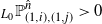 $_{L_{0}}\mathbb{P}^{\hat{n}}_{(1,i), (1,j)}> 0$. Then we have for any
 $j \in \mathbb{N}_{m}$,
 \begin{align*} (F^{(\ell)}_{10}(1)\boldsymbol{1})_{i} &= \sum_{n=\ell}^{\infty} n(n-1)\cdots (n-\ell+1) \mathbb{P}_{(1,i)}\{\tau_{0}=n\} \\* &\geq \sum_{n= \hat{n}}^{\infty} n(n-1)\cdots (n-\ell+1) {_{L_{0}}}P^{\hat{n}}_{(1,i), (1,j)}\mathbb{P}_{(1,j)}\{\tau_{0}=n- \hat{n}\}\\* &\geq {_{L_{0}}}\mathbb{P}^{\hat{n}}_{(1,i), (1,j)} (F^{(\ell)}_{10}(1)\boldsymbol{1})_{j}, \end{align*}
which implies that if 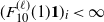 $(F^{(\ell)}_{10}(1)\boldsymbol{1})_{i}<\infty$ for some
 $i \in \mathbb{N}_{m}$, then
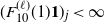 $(F^{(\ell)}_{10}(1)\boldsymbol{1})_{j}<\infty$ for any
 $j \in \mathbb{N}_{m}$. Thus, since
 $\boldsymbol{\mu}^{T}$ is positive and the chain is irreducible, which implies that
 $A_{0}$ is not a zero matrix, we get that
 $(F^{(\ell)}_{10}(1)\boldsymbol{1})_{i}<\infty$ for any
 $i\in \mathbb{N}_{m}$ from
 $\boldsymbol{\mu}^{T} A_{0} F^{(\ell)}_{10}(1)\boldsymbol{1}<\infty$. Differentiating both sides of (30)
 $\ell$ times, we have for
 $\ell\geq 2$
 \begin{equation} F^{(\ell)}_{00}(1)\boldsymbol{1} = \ell \tilde{A}_{0}F^{(\ell-1)}_{10}(1)\boldsymbol{1}+ \tilde{A}_{0}F^{(\ell)}_{10}(1)\boldsymbol{1}.\end{equation}
Thus we derive  $F^{(\ell)}_{00}(1)\boldsymbol{1}<\infty$ from
 $F^{(\ell)}_{10}(1 )\boldsymbol{1}<\infty$. Furthermore, from (27) and (28), we have
 $\sum_{n=1}^{\infty}n^{\ell} \tilde{f}_{00}(n)\boldsymbol{1}<\infty$.
Since the chain is transient, i.e.  $(F_{00}(1)\boldsymbol{1})_{i}<1$ for some
 $i\in \mathbb{N}_{m_{0}}$, from Remark 2 and the fact that
 \begin{equation*}\biggl(\sum_{n=1}^{\infty}n^{\ell} \tilde{f}_{00}(n)\boldsymbol{1}\biggr)_{i}=\mathbb{E}_{(0, i)}[\tau_{L_{0}}^{\ell}1_{\{\tau_{L_{0}}<\infty\}}],\end{equation*}
we obtain that the chain is  $\ell$-transient.
Finally we will show the necessity of (ii). Assume that the chain is  $\ell$-transient and G is irreducible. Then from Proposition 1 (iv) and Proposition 2 (i), we have
 \begin{equation*}\sum_{n=\ell}^{\infty} n(n-1)\cdots (n-\ell+1) \mathbb{P}_{(1,j)}\{\Phi_{n}=(2, j^{\prime})\}<\infty, \quad j, j^{\prime} \in \mathbb{N}_{m}.\end{equation*}
Thus we get
 \begin{align} R^{(\ell)}_{jj^{\prime}} &= \sum_{n=\ell}^{\infty} n(n-1)\cdots (n-\ell+1) \mathbb{P}_{(1,j)}\{\Phi_{n}=(2, j^{\prime}), \Phi_{k}\not\in L_{\leq 1} ,k \in \mathbb{N}_{n-1}\} \notag \\* &\leq \sum_{n=\ell}^{\infty} n(n-1)\cdots (n-\ell+1)\mathbb{P}_{(1,j)}\{\Phi_{n}=(2, j^{\prime})\} \notag \\* &<\infty,\end{align}
which implies that  $G^{(\ell)}<\infty$ according to (15). Since G is irreducible, from the proof of Theorem 2, we know that
 $G^{(\ell)}\boldsymbol{1}<\infty$ if and only if
 $\sum_{v=0}^{\infty}v^{\ell}A_{v}<\infty$. Hence we get the assertion.
Appendix D. Proof of Theorem 5
Proof. The proof of (i) uses the same steps as the proof in Theorem 4. We omit the proof of (i) and only show (ii) and (iii).
(ii) We show that  $P_{GI}$ is not
 $\ell$-transient for any
 $\ell\geq1$. Otherwise, we assume that
 $P_{GI}$ is 1-transient, which implies that
 $R^{(1)}<\infty$ from (37). From (12) we obtain
 \begin{equation}R^{(1)}=\sum_{v=0}^{\infty}R^{v}A_{v}+ \sum_{v=1}^{\infty}\sum_{k=0}^{v-1}R^{k}R^{(1)}R^{v-k-1}A_{v}.\end{equation}
Premultiplying both sides of (38) by  $\boldsymbol{\xi}^{T}(1)$, we get
 \begin{equation}\boldsymbol{\xi}^{T}(1)R^{(1)}=\sum_{v=0}^{\infty}\rho^{v}(1)\boldsymbol{\xi}^{T}(1)A_{v}+ \sum_{v=1}^{\infty}\sum_{k=0}^{v-1}\rho^{k}(1)\boldsymbol{\xi}^{T}(1)R^{(1)}R^{v-k-1}A_{v}.\end{equation}
For  $\boldsymbol{\mu}^{T}\boldsymbol{\nu}= 1$, from Lemma 1 (i) we have
 $\rho(1)=1$. From Remark 4 (ii) we get
 $\boldsymbol{\xi}^{T}(1)=\boldsymbol{\mu}^{T}$. Thus (39) is rewritten as
 \begin{equation}\boldsymbol{\mu}^{T} R^{(1)}\biggl[I-\sum_{k=1}^{\infty}\sum_{m=0}^{k-1}R^{m}A_{k}\biggr]=\boldsymbol{\mu}^{T}.\end{equation}
Define
 \begin{equation*}\sum_{k=1}^{\infty}\sum_{m=0}^{k-1}R^{m}A_{k}= \hat{H}.\end{equation*}
It is obvious that  $\hat{H}$ is a non-negative matrix. From (39), we have
 $\boldsymbol{\mu}^{T} R^{(1)}\hat{H} \leq \boldsymbol{\mu}^{T} R^{(1)}$. Since
 $\boldsymbol{\mu}^{T} R^{(1)}$ and
 $\boldsymbol{\mu}^{T}R^{(1)}\hat{H}$ are non-negative vectors, we have
 $\boldsymbol{\mu}^{T} R^{(1)}\geq \boldsymbol{\mu}^{T}>\boldsymbol0^{T}$. Thus, from Lemma* in [Reference Debreu and Herstein7, page 601], we have that the spectral radius of
 $\hat{H}$ is no more than 1. Now we will show that the spectral radius of
 $\hat{H}$ is equal to 1. From Proposition 4, we have
 \begin{equation} R^{n}=\Delta^{-1}(G^{T})^{n}\Delta.\end{equation}
Since  $\boldsymbol{\mu}^{T}\boldsymbol{\nu}=1$, and A and G are irreducible, we have that G is stochastic. From equation (3.1.5) in [Reference Neuts29], we know that
 \begin{equation*} \lim_{n\rightarrow \infty}(G^{T})^{n}=(\boldsymbol{1}\boldsymbol{g}^{T})^{T}, \end{equation*}
where  $\boldsymbol{g}^{T}$ is the invariant probability vector of G. Combining with (41), we have
 \begin{equation*}\lim_{n\rightarrow \infty}R^{n}= \Delta^{-1}(\boldsymbol{1}\boldsymbol{g}^{T})^{T}\Delta= \Delta^{-1}\boldsymbol{g}\boldsymbol{\mu}^{T},\end{equation*}
which implies that  $[I-R+\Delta^{-1}\boldsymbol{g} \boldsymbol{\mu}^{T}]^{-1}$ exists. From (12), we have
 \begin{equation*} [I-R+\Delta^{-1}\boldsymbol{g} \boldsymbol{\mu}^{T}]\biggl(I-\sum_{k=1}^{\infty}\sum_{m=0}^{k-1}R^{m}A_{k}\biggr)=I-A+ \Delta^{-1}\boldsymbol{g} \boldsymbol{\mu}^{T}-\Delta^{-1}\boldsymbol{g} \boldsymbol{\mu}^{T}\sum_{k=1}^{\infty}kA_{k} \end{equation*}
and
 \begin{equation*} \biggl[I-A+ \Delta^{-1}\boldsymbol{g} \boldsymbol{\mu}^{T}-\Delta^{-1}\boldsymbol{g} \boldsymbol{\mu}^{T}\sum_{k=1}^{\infty}kA_{k}\biggr]\boldsymbol{1}=0, \end{equation*}
which means that  $I-\hat{H}$ is singular, and thus the spectral radius of
 $\hat{H}$ is equal to 1.
From Theorem I* in [Reference Debreu and Herstein7, page 600], there exists a non-zero right eigenvector  $\boldsymbol{y}$ of
 $\hat{H}$ with eigenvalue 1 satisfying
 $\boldsymbol{y} \geq \boldsymbol{0}$ and
 \begin{equation*} (I-\hat{H})\boldsymbol{y}=\boldsymbol{0}.\end{equation*}
Post-multiplying both sides of (40) by  $\boldsymbol{y}$ leads to a conflict that
 $0=\boldsymbol{\mu}^{T} \boldsymbol{y} \neq 0$. Hence our assumption does not hold, which means that the chain is not 1-transient, that is,
 \begin{equation*}\sum_{n=1}^{\infty}n \tilde{f}_{00}(n)\boldsymbol{1}=\infty.\end{equation*}
Thus, for any  $\ell\geq 2$,
 \begin{equation*}\sum_{n=1}^{\infty}n ^{\ell}\tilde{f}_{00}(n)\boldsymbol{1}=\infty.\end{equation*}
Hence we get assertion (ii).
(iii) Since  $\mathbb{P}_{GI}$ is not stochastic, the chain is transient, we have
 $N_{0}(1)<\infty$ and then
 $n_{0}(1)<\infty$, where
 $n_{0}(s)$ is the maximal eigenvalue of
 $N_{0}(s)$. Let
 $u_{0}(s)$ be the maximal eigenvalue of
 $U_{0}(s)$. From (14) we have
 $n_{0}(s)={{1}/{(1-u_{0}(s))}}.$ Thus we derive
 $u_{0}(1)< 1$ from
 $n_{0}(1)<\infty$.
From (13) we have
 \begin{equation} U_{0}(s)\boldsymbol{1}\leq s D_{0}\boldsymbol{1}+ \sum_{k=1}^{\infty} s\tilde{A}_{0}N(s)R^{k-1}(s)s\boldsymbol{1}.\end{equation}
Since  $\boldsymbol{\mu}^{T}\boldsymbol{\nu}> 1$, using a similar argument to the proof of Theorem 6 in [Reference Bean, Bright, Latouche, Pearce, Pollett and Taylor3], we know that
 $\bar{\alpha}> 1$, where
 $\bar{\alpha}$ is the convergence radius of P. Thus there exists some
 $\hat{s}>1$ such that
 $N(\hat{s})<\infty $. In addition, from Lemma 1 (ii), we get
 $\rho(\hat{s})< 1$. Thus we have
 \begin{align*} \sum_{k=1}^{\infty} \hat{s} \tilde{A}_{0}N(\hat{s})R^{k-1}(\hat{s})\hat{s}\boldsymbol{1} &\leq \sum_{k=1}^{\infty} {\hat{s}}^{2} \tilde{A}_{0}N(\hat{s})R^{k-1}(\hat{s})h\Delta^{-1}\boldsymbol{\zeta}(\hat{s})\\* &= \sum_{k=1}^{\infty} {\hat{s}}^{2} \tilde{A}_{0}N(\hat{s})\rho^{k-1}(\hat{s})h\Delta^{-1}\boldsymbol{\zeta}(\hat{s})\\* &<\infty,\end{align*}
where  $\Delta^{-1}\boldsymbol{\zeta}(\hat{s})$ is the right eigenvector of
 $R(\hat{s})$ associated with
 $\rho(\hat{s})$ and h is a bounded real number such that
 $h\Delta^{-1}\boldsymbol{\zeta}(\hat{s})\geq \boldsymbol{1}$.
Therefore, according to (42), we get  $U_{0}(\hat{s})\boldsymbol{1}< \infty$, which implies that
 $u_{0}(\hat{s})< \infty$ and
 $u_{0}(s)$ is continuous on
 $s\in (0, \hat{s}]$. Thus there exists some
 $s\in (1, \hat{s})$ such that
 $u_{0}(s) < 1$ since
 $u_{0}(1)< 1$ and
 $u_{0}(\hat{s})< \infty$. Then we get
 $n_{0}(s)<\infty$ and
 $N_{0}(s)<\infty$. Hence the chain is geometrically transient and the proof is finished.
Acknowledgements
We would like to thank Professor Yiqiang Q. Zhao for his helpful comments on revised versions of the paper. The second author acknowledges the support from the Faculty of Science at Carleton University during the visit in which this research was completed. This research was supported in part by the National Natural Science Foundation of China (grants 11971486, 11571372, and 11771452) and Natural Science Foundation of Hunan (grants 2019JJ40357 and 2017JJ2328).



