Introduction
Our understanding of exoplanetary atmospheres relies on the remote sensing of radiation that, arising from the host star or the planet itself, becomes imprinted with some of the planet's atmospheric features. Ongoing technological developments, to be implemented in >30-m ground-based telescopes and dedicated space missions, are steadily increasing the number of exoplanets amenable to atmospheric characterization. In the foreseeable future, sophisticated instruments will allow us to separate the radiation of an Earth twin from the glare of its host star (e.g. Traub & Oppenheimer Reference Traub, Oppenheimer and Seager2010, and refs. therein). At that moment, it will be possible to address questions such as the occurrence of life on the planet by searching for selected biosignatures in its reflected and/or emitted spectrum (e.g. Des Marais et al. Reference Des Marais, Harwit, Jucks, Kasting, Lin, Lunine, Schneider, Seager, Traub and Woolf2002; Seager et al. Reference Seager, Turner, Schafer and Ford2005; Sparks et al. Reference Sparks, Hough, Germer, Chen and Dassarma2009; Brandt & Spiegel Reference Brandt and Spiegel2014)
In preparation for that moment, modellers have been setting up and testing the tools with which one day the (one pixel, at first) images of Earth-like exoplanets will be rationalized (e.g. Ford et al. Reference Ford, Seager and Turner2001; Tinetti et al. Reference Tinetti, Meadows, Crisp, Fong and Fishbein2006; Stam Reference Stam2008; Zugger et al. Reference Zugger, Kasting, Williams, Kane and Philbrick2010, Reference Zugger, Kasting, Williams, Kane and Philbrick2011; Karalidi et al. Reference Karalidi, Stam and Hovenier2011, Reference Karalidi, Stam and Hovenier2012; Robinson et al. Reference Robinson, Meadows, Crisp, Deming and A'Hearn2011; Karalidi & Stam Reference Karalidi and Stam2012). As some of those works have shown, the information contained in spectra and colour photometry of the one-pixel images will inform us about aspects of the planet such as its atmospheric composition, existence of clouds, and land/ocean partitioning. A key aspect of models, and one that is investigated here, is their capacity to predict an exoplanet's remote appearance and, in particular, how to treat the three-dimensional nature of the atmospheres. The need for such a treatment becomes more apparent as a number of groups are beginning to explore the coupled effects of atmospheric dynamics, heat redistribution and chemistry in the framework of General Circulation Models (e.g. Joshi Reference Joshi2003; Menou Reference Menou2012; Zalucha et al. Reference Zalucha, Michaels and Madhusudhan2013; Carone et al. Reference Carone, Keppens and Decin2014; Kataria et al. Reference Kataria, Showman, Fortney, Marley and Freedman2014).
Modelling radiative transport in three-dimensional atmospheres is a computationally intensive task. For that reason it is important to explore all possible avenues. The two most usual approaches to the problem are:
-
1. The planet disk is partitioned into an n x × n y number of disk elements. The outgoing radiation is calculated at each discrete element under the approximation of locally plane-parallel atmosphere; then, each discrete contribution is properly added up to generate the disk-integrated magnitude. Its computational cost is proportional to n x × n y . As an example, simulating a fully illuminated planet at the 2° × 2° resolution level involves 8100 separate calculations.
-
2. Disk integration is directly approached by means of Monte Carlo (MC) integration. The MC scheme conducts one-photon numerical experiments, each of them tracing a photon trajectory through the atmospheric medium. Repeating the experiment n ph times results in an estimate of the disk-integrated outgoing radiation that converges to the exact magnitude with a standard deviation that follows a ~n ph −1/2 law. Ford et al. (Reference Ford, Seager and Turner2001) utilized a Forward MC algorithm to investigate the diurnal variability of the Earth's brightness. Forward refers to the tracing of the photons starting from the radiation source onwards through the atmospheric medium, i.e. in the same order as the actual photon displacements. In the MC approach, the total computational cost is proportional to n ph.
Recent work has introduced an alternative approach based on Pre-conditioned Backward Monte Carlo (PBMC) integration of the vector Radiative Transport Equation (García Muñoz & Mills Reference García Muñoz and Mills2014). Past applications of the PBMC model to the problem of scattering from a spatially unresolved planet focused on atmospheres that might be stratified in the vertical but exhibited otherwise uniform optical properties in the horizontal direction. The importance of accounting for three-dimensional effects in the description of the optical properties of exoplanets has been substantiated by a number of works (Ford et al. Reference Ford, Seager and Turner2001; Tinetti et al. Reference Tinetti, Meadows, Crisp, Fong and Fishbein2006; Karalidi & Stam Reference Karalidi and Stam2012; Karalidi et al. Reference Karalidi, Stam and Hovenier2012).
Here, I investigate further the PBMC approach and use it to explore Earth's remote appearance for non-uniform distributions of cloud and surface properties. The methodology may find application in the interpretation of earthshine observations (e.g. Arnold et al. Reference Arnold, Gillet, Lardière, Riaud and Schneider2002; Woolf et al. Reference Woolf, Smith, Traub and Jucks2002; Sterzik et al. Reference Sterzik, Bagnulo and Pallé2012; Bazzon et al. Reference Bazzon, Schmid and Gisler2013) and in related research fields such as climate studies that are concerned with planet-averaged properties. This is ongoing work that demonstrates the potentiality of the PBMC approach to become a reference technique in the production of disk-integrated curves for exoplanets.
Section ‘The PBMC algorithm’ introduces the method, section ‘Atmospheric and surface model’ describes the atmospheric, cloud and surface properties implemented in the current exploration exercise and section ‘Model results’ comments on the phase and diurnal light curves of Earth for a few wavelengths and two different cloud covers. Finally, section ‘Messenger diurnal light curves’ introduces the brightness light curves of Earth obtained with images from the 2005 Earth flyby of the Messenger spacecraft and section ‘Summary and outlook’ summarizes the main conclusions and touches upon follow-up work.
The PBMC algorithm
The fundamentals of the PBMC algorithm have been described (García Muñoz & Mills Reference García Muñoz and Mills2014), and the model has been validated for horizontally uniform atmospheres (García Muñoz & Mills Reference García Muñoz and Mills2014; García Muñoz et al. Reference García Muñoz, Pérez-Hoyos and Sánchez-Lavega2014). The validation exercise included a few thousand solutions from the literature for plane-parallel media, disk-integrated model solutions for Rayleigh-scattering atmospheres and measurements of the disk-integrated brightness and polarization of Venus. In the comparison against other model calculations, typical accuracies of 0.1% and better are achieved.
The algorithm calculates the stellar radiation reflected from the whole disk for planets with stratified atmospheres. The calculation proceeds by simulating a sequence of n ph one-photon numerical experiments. Being a backward algorithm, each experiment traces a photon trajectory from the observer through the scattering medium. The contribution to the estimated radiation as measured by the observer is built up by partial contributions every time the photon undergoes a collision. The simulation stops when the photon is either fully absorbed in or escapes from the atmosphere. Pre-conditioning refers to a novel scheme that incorporates the polarization history of the photon (since its departure from the observer's location) into the sampling of propagation directions. Pre-conditioning prevents spurious behaviours in conservative, optically thick, strongly polarizing media and accelerates the convergence over the non-pre-conditioned treatment.
The algorithm includes a scheme to select the photon entry point into the atmosphere based on the local projected area of the ‘visible’ planet disk (García Muñoz & Mills Reference García Muñoz and Mills2014). This strategy ensures that all simulated photons contribute to the estimated radiation at the observer's location. In this approach, each solution to the radiative problem is specific to the details of the illuminated disk as viewed by the observer. Changing that view requires a new radiative transport calculation. The implementation is based on the vector Radiative Transport Equation, which entails that the model computes the disk-integrated Stokes vector of the planet. Not explored in past applications of the PBMC approach, the model is well suited for investigating planets with non-uniform distributions of clouds and albedos.
Atmospheric and surface model
The PBMC algorithm handles elaborate descriptions of the atmospheric, cloud and surface optical properties of the planet. To keep the number of parameters reasonable, however, it is convenient to introduce various simplifications, which are described in what follows.
The model atmosphere adopted here includes gas and clouds and utilizes a 30-slab vertical grid with resolutions of 1, 2 and 4 km for altitudes in the 0–10, 10–30 and 30–70 km ranges. The gas is stratified with a scale height of 8 km and the total Rayleigh optical thickness is parameterized by τg = 0.1 (0.555/λ [μm])4. Clouds are placed in a single slab and assumed to be composed of liquid water and have wavelength-dependent real refractive indices ranging from 1.34 at 0.47 μm to 1.30 at 2.13 μm. The considered cloud droplet sizes have an effective radius and variance of r eff = 7.33 μm and ν eff = 0.12, respectively, which is appropriate for continental stratus clouds (Hess et al. Reference Hess, Koepke and Schult1998). The scattering matrix for the polarization calculations is determined from Mie theory (Mishchenko et al. Reference Mishchenko, Travis and Lacis2002). The cloud optical thickness τc is assumed to be the same for all clouds on the planet. The model atmosphere includes absorption by ozone in the Chappuis band (Jacquinet-Husson et al. Reference Jacquinet-Husson, Scott, Chédin, Garceran and Armante2005). The ozone vertical profile peaks in the stratosphere at 25 km and has an integrated column of 275 Dobson units (Loughman et al. Reference Loughman, Griffioen, Oikarinen, Postylyakov and Rozanov2004). Ozone absorption is stronger between 0.55 and 0.65 μm, and its effect on the radiative transport calculations is particularly distinct in that spectral range. No other gas molecular bands were considered, and therefore the study focuses on the spectral continuum rather than on strong absorption molecular features. Future work will investigate the potential advantages of introducing the spectral direction into the MC integration. Foreseeably, associating each one-photon experiment with a properly selected wavelength (over an instrument's bandpass) and with a photon entry point into the atmosphere may lead to further computational savings in the simulation of spectra with respect to the usual strategy of stacking many monochromatic calculations and subsequently degrading the so-formed spectrum. The savings are likely to be significant if the final spectra are only required at moderate-to-low resolving powers.
At the planet surface, the model adopts the MODIS white-sky albedos specific to early August 2004 (Moody et al. Reference Moody, King, Platnick, Schaaf and Gao2005)Footnote 1 . The albedos are available at bands centred at 0.47, 0.555, 0.659, 0.858, 1.24, 1.64 and 2.13 μm, which cover much of the spectrum dominated by reflected radiation. The bandwidths of the MODIS filters are of 20–50 nm (Xiong et al. Reference Xiong, Chiang, Sun, Barnes, Guenther and Salomonson2009). The monochromatic model calculations presented here are carried out at the MODIS central wavelengths. The prescribed albedos are identically zero over the ocean. Surface reflection is throughout assumed to be of Lambertian type. Specular reflection at the ocean, which may contribute to the planet signal at large phase angles (Williams & Gaidos Reference Williams and Gaidos2008; Robinson et al. Reference Robinson, Meadows and Crisp2010; Zugger et al. Reference Zugger, Kasting, Williams, Kane and Philbrick2010, Reference Zugger, Kasting, Williams, Kane and Philbrick2011), will be implemented in later work.
The adopted maps of cloud fraction are from MODIS dataFootnote 2 specific to 3rd August 2005 (see section ‘Messenger diurnal light curves’). For each one-photon experiment, a scheme based on the local cloud fraction f c at the photon entry point into the atmosphere determines the surface albedo to be utilized in that specific photon trajectory simulation and whether the photon is traced through a gas-only or gas-plus-cloud medium. Internally, the scheme draws a random number ρc ε [0, 1]. If ρc ≤ f c, the photon is traced through an atmosphere of optical thickness τg + τc with optical properties within each slab properly averaged over the gas and cloud. Otherwise, if ρc > f c, the photon is traced through a gas-only atmosphere of optical thickness τg.
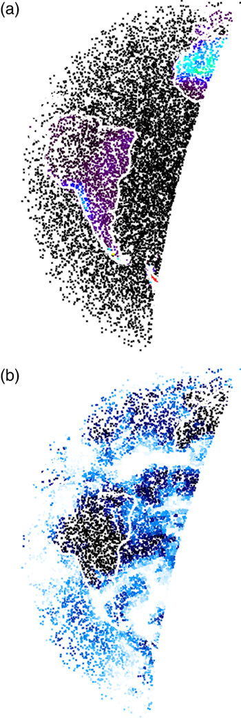
Both the input surface albedo and cloud fraction maps are averaged and mapped onto longitude/latitude maps of 2° × 2° resolution. Each map is read into the model at the beginning of the run and kept in memory throughout the simulation of the n ph one-photon experiments. Figure 1 shows albedo and cloud fraction maps as sampled by the model in a run specific to the Messenger view of Earth on 18:30UT 3rd August 2005.
Top. In the PBMC algorithm, each one-photon experiment is associated with a local albedo value. This image shows the surface albedo at 0.47 μm as sampled in a n ph = 104 calculation for viewing and illumination conditions specific to the Messenger view of Earth on 18:30UT 3rd August 2005. The phase angle for this view of the Earth is equal to 98.7°. The density of sampling points is based on the projected area of the planet's visible disk, which explains why the sampling points tend to concentrate near the terminator. Bottom. Same as above but showing the cloud fraction f c . White and black stand for f c = 1 and = 0, respectively.

Model results
A look into convergence
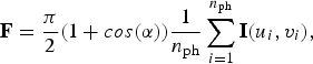
In the implementation of the PBMC algorithm, the irradiance F at the observer's location is evaluated through a summation:
 $${\bf F} = \displaystyle{ {\rm \pi}\over 2}(1 + cos( {\rm \alpha} ))\displaystyle{1 \over {n_{{\rm ph}}}} \sum\limits_{i = 1}^{n_{{\rm ph}}}{\bf I}(u_i, v_i ){\rm,} $$
where I(u i , vi ) is the outgoing radiance Stokes vector from the i-th one-photon experiment, the uniform random variables u, v∈ [0, 1] sample the planet visible disk and α is the star–planet-observer phase angle (García Muñoz & Mills Reference García Muñoz and Mills2014). Equation (1) is effectively an arithmetic average and its convergence properties depend on the dispersion in the outcome of the one-photon experiments. F I is the first element of F and in the adopted normalization it is identical to A g Φ(α), where A g is the planet's geometric albedo and Φ(α) (Φ (0)≡1) is the planet's scattering phase function. Properly, the planet's scattering phase function also depends on the optical properties of the planet as viewed from the observer's location, and they may change over time.
To investigate the convergence properties of F, it is convenient to introduce σ I that defines the standard deviation for the first element I of I after n ph one-photon experiments:
 $${\rm \sigma} _I^2 = \displaystyle{1 \over {n_{{\rm ph}} - 1}}\left( {\displaystyle{1 \over {n_{{\rm ph}}}} \sum\limits_{i = 1}^{n_{{\rm ph}}}\,I_i^2 - \left( {\displaystyle{1 \over {n_{{\rm ph}}}} \sum\limits_{i = 1}^{n_{{\rm ph}}} \,I_i} \right)^2} \right),$$
and where I i is a short form for I(u i , vi ). In turn, for F I :
 $${\rm \sigma} _{F_I} = \displaystyle{{\rm \pi} \over 2}(1 + cos({\rm \alpha} )){\rm \sigma} _I. $$
Analogous expressions can be written for the other elements of F: F Q , FU and F V .
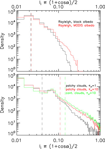
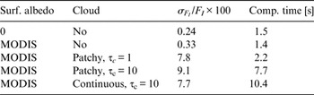
Figure 2 shows histograms of the I i π(1 + cos(α))/2 values obtained in the application of equation (1) to one of the atmospheric configurations discussed in section ‘Messenger diurnal light curves’. The top panel corresponds to Rayleigh atmospheres at 0.48 μm above a black surface (black curve) or above the non-uniform MODIS albedo surface (red curve). A non-uniform surface albedo leads to a slightly broader histogram and a correspondingly larger value of σ F I /F I , as shown in Table 1. σ F I /F I is indeed a measure of the accuracy associated with the estimated F I after n ph one-photon experiments.
Histograms for the partial evaluations of equation (1) with the PBMC algorithm and various surface/cloud configurations. Each experiment comprises a total of n ph = 105 one-photon realizations. The top and bottom panels are specific to cloud-free and cloud-covered atmospheres, respectively. The experiment corresponds to the viewing/illumination geometry of Fig. 1, with α = 98.7°. The dashed vertical lines are mean value estimates for F I , as follows from equation (1).

Summary of performances of the algorithm for disk integration at 0.48 μm and various Earth configurations discussed in section ‘A look into convergence’. Computational times are based on a 2.8 GHz workstation and nph = 105

The bottom panel of Fig. 2 shows the histograms obtained for configurations that in addition incorporate the MODIS cloud map (black and red curves, τc = 1 and 10, respectively) or a continuous cloud cover of optical thickness τc = 10 (green curve). From the comparison of the two panels, it becomes clear that clouds broaden the possible outcome from the single-photon experiments, which affects the accuracy of the algorithm for a prescribed number of one-photon experiments. From the values of σ F I /F I and computational times for n ph = 105 listed in Table 1, it is straightforward to estimate the accuracy and computational time for an arbitrary n ph. In all cases, estimates of F I accurate to within 3% (1%) can be obtained in about 1 (10) minutes. A clear advantage of the current approach is that there is little or no overhead associated with the integration over a non-uniform disk, as shown in Table 1.
Earth simulations from 0.47 to 2.13 μm
Brightness and degree of linear polarization
The number of possibilities to explore in terms of viewing geometries and surface/atmosphere configurations is infinite. Important conclusions for configurations that include polarization have been presented in the literature (e.g. Bailey Reference Bailey2007; Stam Reference Stam2008; Zugger et al. Reference Zugger, Kasting, Williams, Kane and Philbrick2010, Reference Zugger, Kasting, Williams, Kane and Philbrick2011; Karalidi et al. Reference Karalidi, Stam and Hovenier2011, Reference Karalidi, Stam and Hovenier2012; Karalidi & Stam Reference Karalidi and Stam2012). To demonstrate the PBMC algorithm, here I will focus on the impact of the cloud optical thickness and adopt τc = 0 and 5 for two separate sets of calculations. It is assumed that the planet follows an edge-on circular orbit with the sub-observer point permanently on the equator of the planet. Because with the present definition of F Q and F U , the relation |F U |≪|F Q | generally holds (see section ‘Brightness and degree of linear polarization’), only F I and F Q /F I are considered here.
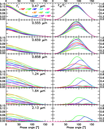
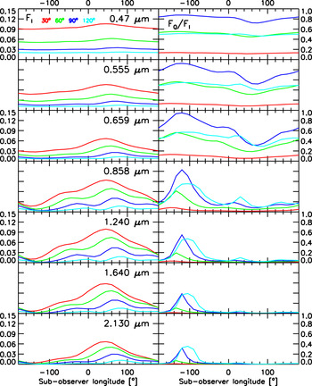
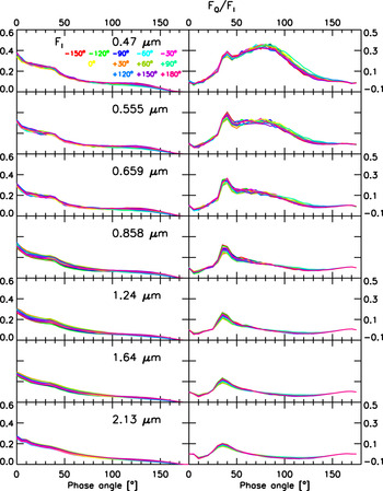
Figure 3 corresponds to τc = 0 (brightness F I on the left and polarization F Q /F I on the right) and shows essentially Rayleigh-scattering phase curves (Buenzli & Schmid Reference Buenzli and Schmid2009). The cloud-free calculations were carried out with n ph = 105, which entails that the results are accurate to better than 1%. For each wavelength, the different colour curves correspond to different sub-observer longitudes. Local changes in the albedo (and in particular, whether land/ocean dominate the field of view) modulate both the brightness and polarization of the planet. The modulation is stronger at the longer wavelengths because the Rayleigh optical thickness drops rapidly with wavelength. Figure 4 substantiates the dependence of F I and F Q /F I on the sub-observer longitude, or equivalently, on local time.
Brightness (left) and polarization (right) curves for cloud-free conditions. Only the α = 0–180° range is presented. From top to bottom, wavelengths from 0.47 to 2.13 μm. Within each panel, the different colour curves refer to different sub-observer longitudes.

Brightness (left) and polarization (right) curves for cloud-free conditions. Equivalent to Fig. 5 but substantiating modulations with sub-observer longitude or, equivalently, with local time. Within each panel, the different colour curves refer to different phase angles.

Equivalent to Fig. 3 but for an atmosphere partially covered by clouds of optical thickness τ c = 5. The estimated relative accuracy is 3 and 6% for brightness and polarization.

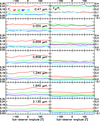
Figures 5 and 6 are analogous to Figs. 3 and 4 but incorporate the MODIS map of cloud fractions for 3rd August 2005, clouds located at 2–3 km altitude and optical thickness τ c ~5. The implemented cloud droplets’ scattering cross-sections vary by less than 10% from 0.47 to 2.13 μm, which justifies the adoption of a wavelength-independent optical thickness for the clouds. The calculations were carried out with n ph = 106 to ensure relative accuracies σ F I /F I ~3%. In the comparison between the cloud-free and cloud-covered configurations, two basic conclusions emerge. First, the curves for τc = 5 show a dependence with phase angle that reveals some basic properties of the scattering cloud particles. Indeed, the polarization phase curves show a peak at α = 30–40° due to the primary rainbow of water droplets (Bailey Reference Bailey2007; Stam Reference Stam2008; Karalidi et al. Reference Karalidi, Stam and Hovenier2011, Reference Karalidi, Stam and Hovenier2012). Second, clouds attenuate much of the diurnal variability and, typically, the diurnal modulation in brightness is easier to pick up than the modulation in polarization.
Equivalent to Fig. 4 but for an atmosphere partially covered by clouds of optical thickness τ c = 5. The estimated relative accuracy is 3 and 6% for brightness and polarization.

Stam (Reference Stam2008) and follow-up work (Karalidi et al. Reference Karalidi, Stam and Hovenier2011, Reference Karalidi, Stam and Hovenier2012; Karalidi & Stam Reference Karalidi and Stam2012) have explored the appearance in both brightness and polarization of Earth-like exoplanets. Stam (Reference Stam2008) and Karalidi et al. (Reference Karalidi, Stam and Hovenier2011) introduce the concept of quasi-horizontally inhomogeneous planets, which allows them to estimate the outgoing radiation from a horizontally non-uniform planet as a weighted sum of the signal from uniform-planet solutions. Their weighting scheme is based on the fractional coverage of each uniform configuration. Karalidi & Stam (Reference Karalidi and Stam2012) and Karalidi et al. (Reference Karalidi, Stam and Hovenier2012), however, utilize a fully inhomogeneous treatment of the planet.
Comparison of Fig. 13 of Stam (Reference Stam2008) at wavelengths of 0.44 and 0.87 μm and Fig. 4 here at wavelengths of 0.47 and 0.858 μm is relevant. For cloud-free conditions and a phase angle α = 90°, F I ~0.03–0.04 and F Q /F I ~0.8 at the shorter wavelength in both works. At the longer wavelength, also for α = 90°, Stam (Reference Stam2008) reports three distinct peaks at different sub-observer longitudes and highest F I values of 0.06. The three-peak structure is reproduced by the calculations presented here, but the highest F I here is 0.045, somewhat lower than 0.06 in Stam (Reference Stam2008). The different treatment of the albedo in the two works, in particular their magnitudes and the absence of Fresnel reflection in the current one, is a likely reason for the discrepancy. In polarization, both works show clear structure that correlates inversely with the brightness. The intensity of the F Q /F I peaks, however, differs between the two works. Since high F Q /F I values typically match dark areas of the planet, again, the discrepancies between the two works probably arise from the different treatment of the surface albedo.
Similarly, comparison of Fig. 14 of Stam (Reference Stam2008) and Fig. 6 here reveals information about the role of clouds. It is difficult to draw definite conclusions from the comparison between the two sets of curves because the optical thickness and droplet size of the clouds implemented in each work are different. The two sets show, however, that the diurnal variability of both F I and F Q /F I is highly attenuated at the shorter wavelength, but that the variability in F I is still distinct at the longer one.
Karalidi & Stam (Reference Karalidi and Stam2012) and Karalidi et al. (Reference Karalidi, Stam and Hovenier2012) investigate further the simulated signal from Earth-like exoplanets and take into account non-uniform cloud and albedo properties. Karalidi et al. (Reference Karalidi, Stam and Hovenier2012) consider a realistic cloud map based on MODIS data. Their work emphasizes the detectability of features like the primary rainbow, which originates from Mie scattering in spherical droplets but may be masked by scattering in ice particles; and, the impact of non-uniformities on the disk-integrated signal. A case-by-case comparison between those works and the results presented in Figs. 3–6 here is not feasible. It is worth noting, nevertheless, that the main features that appear in the curves of Figs. 5 and 6 here are also found in Figs. 6–8 of Karalidi et al. (Reference Karalidi, Stam and Hovenier2012). This includes the occurrence of the primary rainbow in both F I and F Q /F I . The significant variety in the curves reported in those works and here illustrates the complexity of the problem. It also cautions against quick conclusions when the time comes that either brightness or polarization curves of Earth-like exoplanets become available.
The near infrared (e.g. 1.55–1.75; 2.1–2.3 μm) has been proposed as a better option than visible wavelengths in the characterization of surface features that might occur at specific local times (high/low reflecting surfaces such as desert/ocean, respectively) and phase angles (specular reflection from an ocean) (Zugger et al. Reference Zugger, Kasting, Williams, Kane and Philbrick2011). The simulations here (see curves for λ > 1 μm in Figs. 3 and 5) confirm (compare to Fig. 3 in Zugger et al. (Reference Zugger, Kasting, Williams, Kane and Philbrick2011)) that contrasts in the near infrared can be high for cloud-free conditions, but become less distinct at moderate cloud opacities. Since the current implementation of the PBMC model does only account for Lambert reflection at the surface, a more direct comparison with Zugger et al. (Reference Zugger, Kasting, Williams, Kane and Philbrick2011) is not immediately possible.
Angle of linear polarization
Non-uniform surface albedos and patchy clouds introduce an asymmetry between the northern and southern hemispheres that may lead to non-zero values of F U . The angle of polarization χ, defined through tan 2χ = F U /F Q , expresses the orientation of the outgoing polarization vector with respect to the reference plane. The reference plane is normal to the planet scattering plane; the latter is formed by the viewing and illumination directions. Because each photon is tracked with respect to the same three-dimensional absolute rest frame and the same reference plane is utilized to express the Stokes vector, all the photons’ Stokes vectors can be added without further manipulation. The model calculations presented above show, however, that the hemispherically averaged U components take different signs at the northern and southern hemispheres and that summation over the entire disk leads to the effective cancellation of F U , i.e. |F U /F Q |≪1 away from the neutral points where F Q ≈ 0.
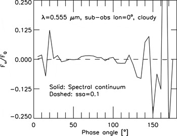
For reference, Fig. (7; solid curve) shows the change in the ratio F U /F Q with phase angle at a wavelength of 0.555 μm and sub-observer longitude of 0° in one of the cloud-covered configurations investigated in Fig. 5. The ratio F U /F Q remains small at all phase angles, with deviations to that trend arising where F Q becomes small and the statistical errors large. Thus, the planet's polarization vector is preferentially aligned with the planet scattering plane (if F Q < 0) or with the reference plane (if F Q > 0), also in the presence of non-uniformities at both the surface and cloud levels.
It is possible to assess what occurs within a molecular absorption band by setting the single scattering albedo in the atmospheric model ϖ < 1. The dashed curve in Fig. 7 presents the ratio F U /F Q for an adopted ϖ = 0.1 at all altitudes. In those conditions, single scattering dominates and the ratio F U /F Q becomes smaller. According to the calculations shown in Fig. 7, the angle of linear polarization χ is either close to zero or to π/2 both within and outside molecular absorption bands.
Solid curve: ratio F U /F Q versus phase angle for the cloudy configuration described in Fig. 5 at a wavelength of 0.555 μm and a sub-observer longitude of 0°. The ratio remains close to zero for most phase angles; deviations to that trend are largely due to F Q values nearing zero. Dashed curve: ratio F U /F Q in the same configuration but with a prescribed atmospheric single scattering albedo (ssa ≡ ϖ) of 0.1 at all altitudes. By minimizing the significance of multiple scattering, the dashed curve provides a better insight into conditions within a strong molecular absorption band.

Circular polarization
Circular polarization in the light scattered from planetary atmospheres typically results from two or more collisions of the photons within the medium. In the cases that measurements have been attempted (e.g. Kemp et al. Reference Kemp, Wolstencroft and Swedlund1971; Swedlund et al. Reference Swedlund, Kemp and Wolstencroft1972; Sparks et al. Reference Sparks, Hough and Bergeron2005), the degree of circular polarization is orders of magnitude smaller than for linear polarization, which entails that observations of circular polarization are challenging.
Unlike abiotic material, living organisms may lead to distinct circular polarization signatures (e.g. Sparks et al. Reference Sparks, Hough, Germer, Chen and Dassarma2009) potentially amenable to remote sensing. Indeed, the prospects of using circular polarization as a biomarker in the investigation of habitable exoplanets have prompted new research on this front (e.g. Sparks et al. Reference Sparks, Hough, Germer, Chen and Dassarma2009; Nagdimunov et al. Reference Nagdimunov, Kolokolova and Mackowski2014).
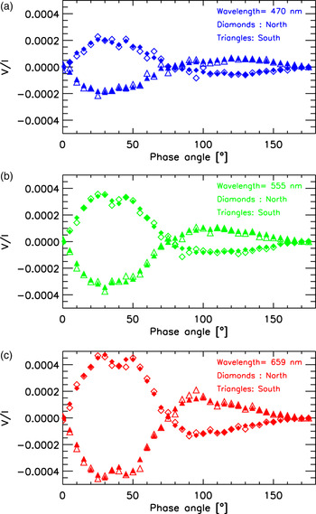
The Earth model considered here does not include circular polarization effects associated with living organisms. It is relevant, nevertheless, to assess the suitability of the PBMC algorithm for a prospective investigation of biogenic circular polarization. On the basis of the configurations investigated in Fig. 5 for cloudy atmospheres, I have calculated F V /F I versus phase angle at the wavelengths of 0.470, 0.555 and 0.659 μm and a sub-observer longitude of 0°. The calculations are presented in Fig. 8 separately for the northern and southern hemispheres, and with n ph = 109 and 1010 one-photon experiments per phase angle. As expected (Kemp et al. Reference Kemp, Wolstencroft and Swedlund1971; Kawata Reference Kawata1978), the two hemispheric components have comparable magnitudes but opposite signs, and tend to cancel out when the integration is extended over the entire planet disk. The numerical experiments suggest that a number n ph = 109 of one-photon numerical experiments are needed to reach acceptable accuracies. This is about three orders of magnitude more than the needs for linear polarization, which conveys one of the difficulties in predicting and interpreting circular polarization features.
Degree of circular polarization V/I for the cloudy configuration described in Fig. 5 at the three specified wavelengths and a sub-observer longitude of 0°. Separate curves are shown for calculations over the northern and southern hemispheres. Open and filled symbols correspond to calculations with n ph of about 109 and 1010, respectively.

Messenger diurnal light curves
On cruise towards Mercury, the NASA Messenger spacecraft performed an Earth flyby in August 2005 (McNutt et al. Reference McNutt, Solomon, Grant, Finnegan and Bedini2008). Observations of Earth during the gravity assist include imagery with the Mercury Dual Imaging System (MDIS) cameras. Of particular interest here are the colour sequences of full-disk images captured with the Wide Angle Camera (WAC) on the departure leg. Each sequence comprises nearly simultaneous observations over a narrow-band filter of band centre/width (μm), λ/Δλ = 0.480/0.01, 0.560/0.006 and 0.63/0.0055. With a cadence of three images every 4 min, the total number of images amounts to 1080.
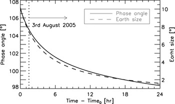
As the spacecraft departs, the Earth angular diameter evolves from 10.2° (nearly filling the WAC field of view of 10.5°) at the start of the sequence to 1.6° at the end of the sequence 24 h later. At its farthest during the sequence (about 457 000 km from Earth), the spacecraft is beyond the Moon orbit. Correspondingly, the Sun-planet centre-spacecraft phase angle α varies from 107° to 98°. Figure 9 presents the two geometric parameters against time since the start of the sequence on 2nd August at about 22:31UT.
Sun–Earth centre-spacecraft phase angle and apparent angular size of Earth during the Messenger flyby.

The WAC images were downloaded from the Planetary Data System and read with the software made available at the Small Bodies NodeFootnote 3 . The basic treatment of the images is similar to that outlined by Domingue et al. (Reference Domingue, Vilas, Holsclaw, Warell and Izenberg2010) in their analysis of the whole-disk optical properties of Mercury. Integration of the planet brightness was conducted over a rectangular box that contains the Earth visible disk. Residual background values were estimated from two stripes running north–south on each side of the box. When possible, the box was designed to extend beyond the visible edge by 0.2–0.3 Earth radii, and the adjacent stripes were 10 pixel wide. Other combinations of box size and stripe width resulted in very similar conclusions. The corrected brightness was then summed over the integration box and multiplied by the solid angle per pixel to yield the planet's irradiance as measured from the spacecraft vantage point, F p . To derive the planet phase function A g Φ, I applied the equation:
 $$F_p = \left( {\displaystyle{{R_p} \over \Delta}} \right)^2 \left( {\displaystyle{1 \over {a_{\rm \star} [{\rm AU}]}}} \right)^2 A_g \Phi F_{\rm \star}, $$
where R p is the Earth's mean radius ( = 6371 km), Δ is the spacecraft-to-Earth centre distance and a ⋆ is the Earth's orbital distance. F ⋆ is the solar irradiance at 1 Astronomical Unit specific to the camera filter (Mick et al. Reference Mick, Murchie, Prockter, Rivkin, Guinness and Ward2012). A related magnitude, the apparent albedo, can be obtained from:
 $$A_{{\rm app}} = \displaystyle{{A_g \Phi (\alpha )} \over {(A_g \Phi (\alpha ))_{{\rm Lambert}}}} = \displaystyle{{A_g \Phi (\alpha )} \over {\displaystyle{2 \over 3}\displaystyle{1 \over \pi} [\sin \alpha + (\pi - \alpha )\cos \alpha ]}},$$
that refers A g Φ(α) to that for a Lambert sphere.
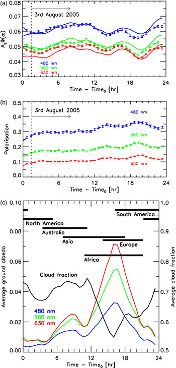
Figure 10 shows the Messenger A g Φ light curves (top panel; solid) against time for each colour filter. For comparison, Mallama (Reference Mallama2009) reports A g Φ(90°) = 0.06 and A g Φ(120°) = 0.05 from earthshine observations in broadband visible light (Goode et al. Reference Goode, Qiu, Yurchyshyn, Hickey and Chu2001). The Messenger curves exhibit variations of peak-to-peak amplitude up to ~20% over times of hours, which is consistent with the findings by EPOXI (Livengood et al. Reference Livengood, Deming, A'Hearn, Charbonneau and Hewagama2011).
Top panel: messenger diurnal light curves. Solid curves are messenger data; dashed curves are model predictions with clouds at 2–3 km altitude and cloud optical thickness τ c = 3. For the model predictions, the error bars are standard deviations σ FI /F I ~1%. Middle panel: model-predicted polarization light curves for the configuration of the top panel. Bottom panel: Average cloud fraction and surface albedos over the Earth visible disk at each instant during the observing sequence.

The evolving phase angle precludes an interpretation of the light curves based solely on diurnal changes in the Earth cover. A detailed observation-model analysis is deferred to future work. It is worth noting, however, that the model captures the major features in the Messenger light curves. Using the atmosphere/surface prescriptions of section ‘Atmospheric and surface model’ (and in particular, the albedo maps at 0.47, 0.555 and 0.658 μm, the latter being somewhat off-set from the MDIS/WAC band centre), the Messenger A g Φ points are reasonably well reproduced by the model calculations (Fig. 10; top panel; dashed) that incorporate the MODIS cloud map specific to 3rd August 2005, clouds located at 2–3 km altitude and optical thickness τ c ~3, an average ozone profile, and the relevant viewing/illumination geometry. The space of model parameters is vast and other atmospheric configurations can plausibly lead to similar or better fits. At the relevant phase angles, the model predicts strong polarization at all three wavelengths, as shown in Fig. (10; middle panel). The model calculations were made with n ph = 107, which entails standard deviations σ F I /F I ~σ F Q /F Q ~1%. The bottom panel of Fig. 10 shows the corresponding cloud fraction and surface albedos averaged over the Earth visible disk at each instant during the observing sequence. The drop in cloudiness and increase in surface albedo that occurs half way through the observing sequence, especially at the longer wavelengths, reveals the presence of Africa's vast desert expanses.
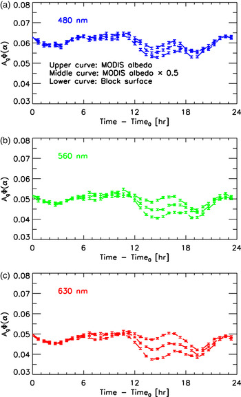
In preparation of a more thorough exploration, Fig. 11 investigates the sensitivity of the model-predicted Messenger light curves to the surface albedo. Postulated changes in the reflective properties of the surface are particularly clear from 12 to 20 h in the observing sequence. This is related to two different factors, namely the low cloud fraction and high surface albedos at the time. Decreased Rayleigh scattering allows photons to penetrate deeper, which leads to increased relative contrasts at the longer wavelength. The simulation above a black surface clearly demonstrates that most, but not all, of the variability in the light curve at the three wavelengths originates from cloud patchiness.
Model-predicted brightness light curves for conditions specific to the Messenger observing sequence. The three curves in each panel represent three differently scaled versions of the surface albedo. The surface becomes more apparent between 12 and 20 h, with Africa well into the field of view, because the cloud fraction is lower and the surface albedo is higher. The contrast is higher at 630 nm than at either 480 or 560 nm because Rayleigh scattering becomes less efficient at longer wavelengths and more photons penetrate deeper into the atmosphere.

Summary and outlook
Models will play key roles in the interpretation of future observations of exoplanetary atmospheres. Here, I presented a method to predict the disk-integrated Stokes vector of stellar radiation reflected from a planet. The method is flexible and handles variations in the planet optical properties in both the vertical and horizontal directions. A strength of this approach is that its computational cost is not significantly affected by non-uniformities at the atmospheric and cloud levels. Being based on MC integration, the accuracy (and in turn, the computational time) of a calculation can be established a priori. Typically, solutions for a specific viewing/illumination geometry accurate to within 3% are produced in 1 min or less for planet configurations as elaborate as those described here for an Earth replica. In the future, it will be interesting to address a detailed analysis of the Messenger light curves and investigate the complementarity of brightness and polarization measurements in the characterization of Earth-like exoplanets over long time baselines.
Acknowledgements
I gratefully acknowledge the assistance of Jake Ritchie (University of Maryland, MD) with the software for reading the Messenger/MDIS images, and access to the GeoViz software (Henry Throop, http://soc.boulder.swri.edu/nhgv/) for the visualization of Earth from the Messenger trajectory. The Messenger/MDIS images were downloaded from the Planetary Data System. I gratefully acknowledge conversations with Tom Enstone (ESA/ESTEC, Netherlands) about the Earth simulations. Finally, I thank Frank P. Mills (Australian National University, Australia) for comments on an early version of the manuscript.