1. Introduction
Homogeneous anisotropic turbulence is a very important topic in turbulence theory, since it allows for a detailed analysis of linear and nonlinear effects of the mean-flow gradient on turbulence dynamics. A key point is the description of anisotropy, and the derivation of evolution equations that retain most of the structural and dynamical information on the flow evolution. The usual starting point for Fourier-space description is to consider the spectral tensor
 $\hat{\unicode[STIX]{x1D619}}_{ij}(\boldsymbol{k},t)$
, which is defined as the Fourier transform of the two-point second-order correlation tensor
 $\unicode[STIX]{x1D619}_{ij}(\boldsymbol{r},t)=\langle u_{i}(\boldsymbol{x},t)u_{j}(\boldsymbol{x}+\boldsymbol{r},t)\rangle$
. Evolution equations can be found for this tensor, which require some closures for nonlinear cubic terms and pressure–velocity correlation terms. A few closed forms have been proposed based on Heisenberg’s transfer models, e.g. Canuto & Dubovikov (Reference Canuto and Dubovikov1996a
,Reference Canuto and Dubovikov
b
,Reference Canuto and Dubovikov
c
). These models do not give a detailed insight into anisotropy, since they rely on a strictly isotropic transfer term as in homogeneous isotropic turbulence. A more general model can be obtained using higher-order closures in place of the quasilocal energy flux, as illustrated in Weinstock (Reference Weinstock2013), who used the eddy-damped quasinormal Markovian (EDQNM) closure for the isotropic turbulence of Orszag (Reference Orszag1970) to derive expressions for the nonlinear transfer term and the nonlinear pressure–strain contribution. This work also relies on an exact treatment of the linear operators induced by mean-velocity gradients in the governing equation for the spectral tensor
 $\hat{\unicode[STIX]{x1D619}}_{ij}(\boldsymbol{k},t)$
, which is permitted by the
 $\boldsymbol{k}$
-space level of description of the proposed model. The latter was used to perform an exhaustive analytical study of homogeneous turbulence subjected to a constant pure plane shear without limitations on time or wavenumber.
As in Weinstock (Reference Weinstock2013), this level of description in
 $\boldsymbol{k}$
-space is the first step of the present model, which entirely includes the nonlinear closure for transfer terms. First, instead of considering the spectral tensor with all of its components, we use its decomposition in terms of directional anisotropy and polarization anisotropy (Cambon & Rubinstein Reference Cambon and Rubinstein2006). A more general representation, say
 $(\mathscr{E},Z,\mathscr{H})(\boldsymbol{k},t)$
, first introduced by Cambon & Jacquin (Reference Cambon and Jacquin1989), also includes a helicity contribution generated by a helicity spectrum
 $\mathscr{H}(\boldsymbol{k},t)$
. The helicity spectrum, which is associated with the imaginary part of
 $\hat{\unicode[STIX]{x1D619}}_{ij}(\boldsymbol{k},t)$
, is not considered here because it remains zero in homogeneous turbulence if it is not initialized or forced, usually in an unphysical way (see also the trivial helicity equation in Cambon & Jacquin (Reference Cambon and Jacquin1989) and Cambon et al. (Reference Cambon, Danaila, Godeferd and Scott2013)). In addition to their mathematical origin, the recourse to the two different terms
 $\mathscr{E}(\boldsymbol{k},t)$
and
 $Z(\boldsymbol{k},t)$
has physical meaning. For instance, the structure-based single-point modelling of Kassinos, Reynolds & Rogers (Reference Kassinos, Reynolds and Rogers2001) can be related to these spectra, the dimensionality tensor being derived from the angular dependence of
 $\mathscr{E}(\boldsymbol{k},t)$
, and the stropholysis tensor from
 $Z(\boldsymbol{k},t)$
. This structure-based modelling is in contrast to other single-point models where anisotropy is characterized by the sole deviatoric tensor associated with the Reynolds stress tensor which is used to express the ‘rapid’ and ‘slow’ parts of the pressure–strain rate tensor. The linkage between our spectral approach based on the directional–polarization anisotropy decomposition and the structure-based single-point modelling of Kassinos et al. (Reference Kassinos, Reynolds and Rogers2001) is detailed in appendix A of the present paper, along with discussions concerning other single-point models.
The compact decomposition of the spectral tensor discussed above simplifies, without any loss of generality, the derivation of dynamical equations, here Lin equations for
 $\mathscr{E}(\boldsymbol{k},t)$
and
 $Z(\boldsymbol{k},t)$
, and that of closure relations. On the other hand, the numerical treatment of the angular dependence of
 $\mathscr{E}(\boldsymbol{k},t)$
and
 $Z(\boldsymbol{k},t)$
remains a challenge. As an example, the numerical cost of axisymmetric EDQNM models (Godeferd & Cambon Reference Godeferd and Cambon1994; Bellet et al.
Reference Bellet, Godeferd, Scott and Cambon2006; Favier et al.
Reference Favier, Godeferd, Cambon, Delache and Bos2011) is much higher than that of the basic EDQNM for isotropic turbulence. These models were developed, from the first case of rotating turbulence (Cambon & Jacquin Reference Cambon and Jacquin1989), for flows dominated by interacting dispersive waves and without explicit linear effect in the governing equation for the energy density
 $\mathscr{E}(\boldsymbol{k},t)$
, requiring the use of the most complicated EDQNM version to handle the effects induced by the mean flow on triple correlations, such as the inhibition of the energy cascade in the case of rotating flows. This configuration is no longer considered here, and we focus in the present paper on turbulent flows interacting with mean-velocity gradients with a symmetric part, hence leading to energy production. At least for the flow configurations considered in this paper (turbulent flows in the presence of mean strain/shear), these production effects induced by the mean flow, which originate from the linear contributions in the equations for second-order correlations, prevail in the evolution of anisotropy compared with the ones that affect triple correlations (Sagaut & Cambon Reference Sagaut and Cambon2008). A self-consistent nonlinear model will be built accordingly, based on fully tensorial EDQNM closure for an arbitrary anisotropic second-order spectral tensor but with no explicit mean-gradient effect in the expression of the nonlinear transfer terms.
Our second step for deriving our final model equations does not include further closure assumptions, it is purely technical but essential to derive a tractable model, especially in terms of numerical treatment. The computational cost of the models in 3D Fourier space discussed above can be significantly reduced by deriving a 1D problem through integration over spheres with arbitrary radius in Fourier space,
 $S_{k}$
. This yields expressions of governing equations for the spherically averaged tensor
 ${\it\varphi}_{ij}(k,t)=\iint _{S_{k}}\hat{\unicode[STIX]{x1D619}}_{ij}(\boldsymbol{k},t)\,\text{d}^{2}\boldsymbol{k}$
that depend on the wavevector modulus,
 $k$
, instead of
 $\boldsymbol{k}$
. This was done by Clark & Zemach (Reference Clark and Zemach1995) in their diffusion-approximation-based model, where the prescription of a scale-dependent relaxation rate leads to satisfactory comparisons with experimental data and to a good description of partial return to isotropy, which is confirmed in, e.g., Chasnov (Reference Chasnov1995). However, discussions in Choi & Lumley (Reference Choi and Lumley2001), Kassinos et al. (Reference Kassinos, Reynolds and Rogers2001) and Zusi & Perot (Reference Zusi and Perot2013, Reference Zusi and Perot2014) about possible nonlinear return to isotropy can eventually motivate the use of anisotropic EDQMN closure and the distinction between directional anisotropy and polarization anisotropy. One can also mention the model of Cambon, Jeandel & Mathieu (Reference Cambon, Jeandel and Mathieu1981), where a closure for nonlinear terms using anisotropic EDQNM was proposed, but without a separation of directional anisotropy and polarization anisotropy. Spherical integration requires a parametrization of the second-order spectral tensor to restore at least a part of its angular dependence, leading to a mathematically consistent model reduced to spherically averaged descriptors. This will be done in our final model by using truncated expansions in terms of angular harmonics of the second-order spectral tensor. A similar approach was considered by Herring (Reference Herring1974) in the context of the direct-interaction approximation (DIA) of Kraichnan (Reference Kraichnan1959). In this work, the question of the number of spherical harmonics necessary to accurately describe the return to isotropy of axisymmetric turbulence is investigated numerically, and a scale-by-scale relaxation rate is identified. This truncation of spherical harmonic series lies at the origin of a loss of information that restricts the present model to moderate anisotropy. Realizability conditions will be considered in order to quantify the upper boundary of anisotropy intensity that can be investigated with the proposed model. A complementary approach to the models described above can be found in Kassinos & Akylas (Reference Kassinos and Akylas2012), where explicit angular dependence is preserved, whereas scale information is lost after integration along rays of fixed orientation in Fourier space.
The key spherical descriptors of our spectral model are now introduced. Starting from a trace–deviator splitting of the real part of the spectral tensor
 $\hat{\unicode[STIX]{x1D619}}_{ij}(\boldsymbol{k},t)$
restricted to the plane normal to the wavevector
 $\boldsymbol{k}$
by virtue of incompressibility,
 $$\begin{eqnarray}\displaystyle \hat{\unicode[STIX]{x1D619}}_{ij}(\boldsymbol{k},t)=\frac{1}{2}\hat{\unicode[STIX]{x1D619}}_{nn}(\boldsymbol{k},t)\unicode[STIX]{x1D617}_{ij}(\boldsymbol{k})+\text{Re}\left(\hat{\unicode[STIX]{x1D619}}_{ij}(\boldsymbol{k},t)-\frac{1}{2}\hat{\unicode[STIX]{x1D619}}_{nn}(\boldsymbol{k},t)\unicode[STIX]{x1D617}_{ij}(\boldsymbol{k})\right),\quad \unicode[STIX]{x1D617}_{ij}(\boldsymbol{k})={\it\delta}_{ij}-\frac{k_{i}k_{j}}{k^{2}}, & & \displaystyle \nonumber\\ \displaystyle & & \displaystyle\end{eqnarray}$$
the following threefold decomposition in terms of isotropic, directional and polarization parts is obtained:
 $$\begin{eqnarray}\hat{\unicode[STIX]{x1D619}}_{ij}(\boldsymbol{k},t)=\underbrace{\frac{E(k,t)}{4{\rm\pi}k^{2}}\unicode[STIX]{x1D617}_{ij}(\boldsymbol{k})}_{\hat{\unicode[STIX]{x1D619}}_{ij}^{(iso)}(\boldsymbol{k},t)}+\underbrace{\mathscr{E}^{(dir)}(\boldsymbol{k},t)\unicode[STIX]{x1D617}_{ij}(\boldsymbol{k})}_{\hat{\unicode[STIX]{x1D619}}_{ij}^{(dir)}(\boldsymbol{k},t)}+\hat{\unicode[STIX]{x1D619}}_{ij}^{(pol)}(\boldsymbol{k},t),\end{eqnarray}$$
by separating the trace of
 $\hat{\unicode[STIX]{x1D619}}_{ij}(\boldsymbol{k},t)$
into purely isotropic and directional anisotropy contributions, according to
 $$\begin{eqnarray}\displaystyle \mathscr{E}(\boldsymbol{k},t)=\frac{1}{2}\hat{\unicode[STIX]{x1D619}}_{nn}(\boldsymbol{k},t),\quad \mathscr{E}^{(dir)}(\boldsymbol{k},t)=\mathscr{E}(\boldsymbol{k},t)-\frac{E(k,t)}{4{\rm\pi}k^{2}},\quad E(k,t)=\iint _{S_{k}}\mathscr{E}(\boldsymbol{k},t)\,\text{d}^{2}\boldsymbol{k}, & & \displaystyle \nonumber\\ \displaystyle & & \displaystyle\end{eqnarray}$$
where
 $E(k,t)$
corresponds to the kinetic energy spectrum. The polarization part
 $\hat{\unicode[STIX]{x1D619}}_{ij}^{(pol)}(\boldsymbol{k},t)$
in (1.2) can be expressed in terms of a complex-valued scalar
 $Z(\boldsymbol{k},t)$
. This decomposition yields the following splitting of the spherically averaged tensor
 ${\it\varphi}_{ij}(k,t)$
:
 $$\begin{eqnarray}{\it\varphi}_{ij}(k,t)=\iint _{S_{k}}\hat{\unicode[STIX]{x1D619}}_{ij}(\boldsymbol{k},t)\,\text{d}^{2}\boldsymbol{k}=2E(k,t)\left(\frac{1}{3}{\it\delta}_{ij}+\unicode[STIX]{x1D60F}_{ij}^{(dir)}(k,t)+\unicode[STIX]{x1D60F}_{ij}^{(pol)}(k,t)\right).\end{eqnarray}$$
The dimensionless deviatoric part of the spherically averaged spectral tensor is therefore
 $\unicode[STIX]{x1D60F}_{ij}(k,t)=\unicode[STIX]{x1D60F}_{ij}^{(dir)}(k,t)+\unicode[STIX]{x1D60F}_{ij}^{(pol)}(k,t)$
, with
 $$\begin{eqnarray}\displaystyle 2E(k,t)\unicode[STIX]{x1D60F}_{ij}^{(dir)}(k,t)=\iint _{S_{k}}\hat{\unicode[STIX]{x1D619}}_{ij}^{(dir)}(\boldsymbol{k},t)\,\text{d}^{2}\boldsymbol{k},\quad 2E(k,t)\unicode[STIX]{x1D60F}_{ij}^{(pol)}(k,t)=\iint _{S_{k}}\hat{\unicode[STIX]{x1D619}}_{ij}^{(pol)}(\boldsymbol{k},t)\,\text{d}^{2}\boldsymbol{k}. & & \displaystyle \nonumber\\ \displaystyle & & \displaystyle\end{eqnarray}$$
The aim of this paper is to propose a model based on the decomposition (1.4) of the averaged tensor
 ${\it\varphi}_{ij}(k,t)$
, yielding a system of 11 equations for the global state vector
 $(E,E\unicode[STIX]{x1D60F}_{ij}^{(dir)},E\unicode[STIX]{x1D60F}_{ij}^{(pol)})(k,t)$
. This system is obtained in two steps. The first step is based on an anisotropic EDQNM closure for the equations that govern the whole spectral tensor
 $\hat{\unicode[STIX]{x1D619}}_{ij}(\boldsymbol{k},t)$
, or equivalently the scalar spectra
 $\mathscr{E}(\boldsymbol{k},t)$
and
 $Z(\boldsymbol{k},t)$
from the directional–polarization anisotropy decomposition. This closure is restricted to flows where linear effects induced by mean-velocity gradients lie at the origin of energy production which prevails in the evolution of anisotropy compared with the induced effects on the dynamics of triple correlations. The mean flow is taken into account through the linear operators, which reflect rapid distortion theory (RDT) if considered alone, in the governing equations for second-order moments, as done in Weinstock (Reference Weinstock2013). The second step consists in parametrizing the angular dependence of
 $\mathscr{E}(\boldsymbol{k},t)$
and
 $Z(\boldsymbol{k},t)$
in terms of the spherically averaged spectral descriptors
 $\unicode[STIX]{x1D60F}_{ij}^{(dir)}(k,t)$
and
 $\unicode[STIX]{x1D60F}_{ij}^{(pol)}(k,t)$
in order to derive a more tractable model in
 $k$
-space. Even if spherical integration entails a loss of information that restricts the present model to moderate anisotropy and prevents a complete resolution of the flow in 3D Fourier space as in Weinstock (Reference Weinstock2013), the model developed in the present paper can be used to calculate homogeneous anisotropic flows in a wide range of configurations, without any restriction to a particular symmetry, including when non-stationary mean-velocity gradients are considered. This point will be illustrated by the different applications of the model considered in this paper.
The paper is organized as follows. In § 2, the governing equations for the spectral tensor
 $\hat{\unicode[STIX]{x1D619}}_{ij}(\boldsymbol{k},t)$
are recalled along with those for the scalar spectra
 $\mathscr{E}(\boldsymbol{k},t)$
and
 $Z(\boldsymbol{k},t)$
. The latter are then closed via an anisotropic EDQNM procedure. The spectral model in terms of spherically averaged descriptors is derived in § 3. Section 4 is devoted to the validation of the present model. To this end, several flow configurations are considered. First, multiple straining processes are addressed and comparisons with various experiments are performed. Several cases of return to isotropy (RTI) are then considered, to assess the capability of the model to account for slow pressure terms and possible lack of RTI with separate investigation of directional anisotropy and polarization anisotropy. The last test case deals with homogeneous turbulence subjected to a constant pure plane shear, to check the capability of the model to recover the asymptotic stage of exponential growth of kinetic energy predicted by, e.g., Weinstock (Reference Weinstock2013). The linkage between single-point models and the model of the present paper is discussed in appendix A.
2. Closed equations for the second-order spectral tensor in sheared turbulence
We consider incompressible homogeneous turbulence. In the presence of a mean-velocity gradient, the Navier–Stokes equation for the fluctuating velocity
 $u_{i}(\boldsymbol{x},t)$
includes additional advection and deformation terms linked to the mean – or large-scale – velocity field
 $U_{i}(\boldsymbol{x},t)$
:
 $$\begin{eqnarray}\left(\frac{\partial }{\partial t}+u_{j}\frac{\partial }{\partial x_{j}}\right)u_{i}+U_{j}\frac{\partial u_{i}}{\partial x_{j}}+\frac{\partial U_{i}}{\partial x_{j}}u_{j}=-\frac{\partial p}{\partial x_{i}}+{\it\nu}{\rm\nabla}^{2}u_{i}.\end{eqnarray}$$
In (2.1),
 $p(\boldsymbol{x},t)$
is the pressure divided by a reference density, and
 ${\it\nu}$
is the kinematic viscosity of the fluid. In § 2.1, we give the governing equation for the second-order spectral tensor
 $\hat{\unicode[STIX]{x1D619}}_{ij}(\boldsymbol{k},t)$
. The (
 $\mathscr{E}$
,
 $Z$
) decomposition is applied to the latter tensor in § 2.2 and to its governing equation in § 2.3. Transfer terms appear from the latter decomposition, which are closed via the EDQNM procedure described in § 2.4.
2.1. Craya’s equations
The mean flow
 $\boldsymbol{U}(\boldsymbol{x},t)$
is characterized by a space-uniform gradient
 ${\it\lambda}_{ij}(t)=(\partial U_{i}/\partial x_{j})(t)$
in accordance with homogeneity for the fluctuations. For the sake of readability, and without loss of generality, we will omit the time dependence of
 ${\it\lambda}_{ij}$
in the following. In anisotropic homogeneous turbulence, all information about two-point second-order correlations is provided by the second-order spectral tensor
 $\hat{\unicode[STIX]{x1D619}}_{ij}(\boldsymbol{k},t)$
, which is the Fourier transform of the two-point second-order correlation tensor
 $\unicode[STIX]{x1D619}_{ij}(\boldsymbol{r},t)=\langle u_{i}(\boldsymbol{x},t)u_{j}(\boldsymbol{x}+\boldsymbol{r},t)\rangle$
, with
 $\boldsymbol{r}$
the vector separating the two points in physical space. This tensor is defined as
 $$\begin{eqnarray}\langle \hat{u} _{i}^{\ast }(\boldsymbol{p},t)\hat{u} _{j}(\boldsymbol{k},t)\rangle ={\it\delta}(\boldsymbol{k}-\boldsymbol{p})\hat{\unicode[STIX]{x1D619}}_{ij}(\boldsymbol{k},t),\end{eqnarray}$$
where
 $\hat{u} _{i}(\boldsymbol{k},t)$
is the Fourier transform of the fluctuating velocity
 $u_{i}(\boldsymbol{x},t)$
, and the operators
 $^{\ast }$
and
 $\langle \,\rangle$
denote complex conjugate and ensemble average respectively. From the counterpart of (2.1) in Fourier space and using definition (2.2) one derives the governing equation for the tensor
 $\hat{\unicode[STIX]{x1D619}}_{ij}(\boldsymbol{k},t)$
(see, e.g., Sagaut & Cambon (Reference Sagaut and Cambon2008)),
 $$\begin{eqnarray}\left(\frac{\partial }{\partial t}-{\it\lambda}_{ln}k_{l}\frac{\partial }{\partial k_{n}}+2{\it\nu}k^{2}\right)\hat{\unicode[STIX]{x1D619}}_{ij}(\boldsymbol{k},t)+\unicode[STIX]{x1D614}_{in}(\boldsymbol{k})\hat{\unicode[STIX]{x1D619}}_{nj}(\boldsymbol{k},t)+\unicode[STIX]{x1D614}_{jn}(\boldsymbol{k})\hat{\unicode[STIX]{x1D619}}_{ni}(\boldsymbol{k},t)=\unicode[STIX]{x1D61B}_{ij}(\boldsymbol{k},t),\end{eqnarray}$$
with the linear operator induced by mean-velocity gradients
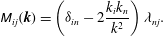 $$\begin{eqnarray}\unicode[STIX]{x1D614}_{ij}(\boldsymbol{k})=\left({\it\delta}_{in}-2\frac{k_{i}k_{n}}{k^{2}}\right){\it\lambda}_{nj}.\end{eqnarray}$$
The transfer tensor
 $\unicode[STIX]{x1D61B}_{ij}(\boldsymbol{k},t)$
in (2.3) accounts for triadic interactions between vectors
 $\boldsymbol{k}$
,
 $\boldsymbol{p}$
and
 $\boldsymbol{q}$
so that they form a triangle. It is possible to disentangle contributions from the tensorial transfer term, with zero integral over
 $\boldsymbol{k}$
, and contributions from the fluctuating pressure
 $\unicode[STIX]{x1D61E}_{ij}(\boldsymbol{k},t)$
as follows:
 $$\begin{eqnarray}\unicode[STIX]{x1D61B}_{ij}(\boldsymbol{k},t)=\unicode[STIX]{x1D617}_{in}(\boldsymbol{k}){\it\tau}_{nj}(\boldsymbol{k},t)\,+\unicode[STIX]{x1D617}_{jn}(\boldsymbol{k}){\it\tau}_{ni}^{\ast }(\boldsymbol{k},t)={\it\tau}_{ij}(\boldsymbol{k},t)+\,{\it\tau}_{ji}^{\ast }(\boldsymbol{k},t)\underbrace{-\frac{k_{i}k_{n}}{k^{2}}{\it\tau}_{nj}(\boldsymbol{k},t)-\frac{k_{j}k_{n}}{k^{2}}{\it\tau}_{ni}^{\ast }(\boldsymbol{k},t)}_{\unicode[STIX]{x1D61E}_{ij}(\boldsymbol{k},t)}.\end{eqnarray}$$
The tensor
 $\unicode[STIX]{x1D61E}_{ij}(\boldsymbol{k},t)$
contains a possible RTI mechanism, its integral over
 $\boldsymbol{k}$
gives the nonlinear – so-called slow – pressure–strain rate tensor, and both the
 $\unicode[STIX]{x1D61B}_{ij}(\boldsymbol{k},t)$
and
 $\unicode[STIX]{x1D61E}_{ij}(\boldsymbol{k},t)$
terms originate from the same tensor
 ${\it\tau}_{ij}(\boldsymbol{k},t)$
. In the same way, the tensor
 ${\it\tau}_{ij}(\boldsymbol{k},t)$
,
 $$\begin{eqnarray}{\it\tau}_{ij}(\boldsymbol{k},t)=k_{n}\iiint \unicode[STIX]{x1D61A}_{ijn}(\boldsymbol{k},\boldsymbol{p},t)\,\text{d}^{3}\boldsymbol{p},\end{eqnarray}$$
is given from the third-order three-point spectral tensor
 $\unicode[STIX]{x1D61A}_{ijn}(\boldsymbol{k},\boldsymbol{p},t)$
, defined by
 $$\begin{eqnarray}\text{i}\langle \hat{u} _{i}(\boldsymbol{q},t)\hat{u} _{j}(\boldsymbol{k},t)\hat{u} _{n}(\boldsymbol{p},t)\rangle ={\it\delta}(\boldsymbol{k}+\boldsymbol{p}+\boldsymbol{q})\unicode[STIX]{x1D61A}_{ijn}(\boldsymbol{k},\boldsymbol{p},t),\end{eqnarray}$$
and the closure is applied to the equation that governs the latter tensor, as shown in § 2.4.
2.2. The
 $(\mathscr{E},Z)$
decomposition

A general decomposition of the second-order spectral tensor
 $\hat{\unicode[STIX]{x1D619}}_{ij}(\boldsymbol{k},t)$
, for arbitrary anisotropy, results from a trace–deviator splitting, restricted to the plane normal to the wavevector
 $\boldsymbol{k}$
by virtue of incompressibility. It is consistent with the threefold decomposition in terms of the isotropic contribution, directional anisotropy and polarization anisotropy, from (1.2) (Cambon & Jacquin Reference Cambon and Jacquin1989; Cambon & Rubinstein Reference Cambon and Rubinstein2006; Sagaut & Cambon Reference Sagaut and Cambon2008). The first term in the decomposition (1.2) of
 $\hat{\unicode[STIX]{x1D619}}_{ij}(\boldsymbol{k},t)$
corresponds to its isotropic part. The second term characterizes ‘directional anisotropy’ via the scalar
 $\mathscr{E}^{(dir)}(\boldsymbol{k},t)=\mathscr{E}(\boldsymbol{k},t)-E(k,t)/(4{\rm\pi}k^{2})$
, which corresponds to the difference between the energy density
 $\mathscr{E}(\boldsymbol{k},t)$
and its spherical average. The third term, which is generated by the scalar
 $Z(\boldsymbol{k},t)$
, characterizes the ‘polarization anisotropy’, or tensorial anisotropy, at a given wavevector.
Following Cambon & Jacquin (Reference Cambon and Jacquin1989), the contribution from the polarization anisotropy is generated by the single complex-valued pseudoscalar term
 $Z(\boldsymbol{k},t)$
as follows:
 $$\begin{eqnarray}\hat{\unicode[STIX]{x1D619}}_{ij}^{(pol)}(\boldsymbol{k},t)=\text{Re}(Z(\boldsymbol{k},t)N_{i}(\boldsymbol{k})N_{j}(\boldsymbol{k})),\end{eqnarray}$$
with
 $$\begin{eqnarray}Z(\boldsymbol{k},t)={\textstyle \frac{1}{2}}\hat{\unicode[STIX]{x1D619}}_{mn}(\boldsymbol{k},t)N_{m}(\boldsymbol{k})^{\ast }N_{n}(\boldsymbol{k})^{\ast },\end{eqnarray}$$
where the vector
 $\boldsymbol{N}(\boldsymbol{k})$
, introduced by Cambon & Jacquin (Reference Cambon and Jacquin1989) and recovered independently by Waleffe (Reference Waleffe1992) as the helical mode, is defined by
 $$\begin{eqnarray}\boldsymbol{N}(\boldsymbol{k})=\boldsymbol{e}^{(2)}(\boldsymbol{k})-\text{i}\boldsymbol{e}^{(1)}(\boldsymbol{k}),\quad \boldsymbol{e}^{(1)}(\boldsymbol{k})=\frac{\boldsymbol{k}\times \boldsymbol{n}}{|\boldsymbol{k}\times \boldsymbol{n}|},\quad \boldsymbol{e}^{(2)}(\boldsymbol{k})=\boldsymbol{e}^{(3)}(\boldsymbol{k})\times \boldsymbol{e}^{(1)}(\boldsymbol{k}),\quad \boldsymbol{e}^{(3)}(\boldsymbol{k})=\frac{\boldsymbol{k}}{k}.\end{eqnarray}$$
Here,
 $(\boldsymbol{e}^{(1)}(\boldsymbol{k}),\boldsymbol{e}^{(2)}(\boldsymbol{k}),\boldsymbol{e}^{(3)}(\boldsymbol{k}))$
is an orthonormal right-handed frame of reference associated with a privileged direction
 $\boldsymbol{n}$
, which is often referred to as the Craya–Herring frame (Herring Reference Herring1974; Sagaut & Cambon Reference Sagaut and Cambon2008). The realizability condition, or condition for the Hermitian covariance matrix
 $\hat{\unicode[STIX]{x1D64D}}(\boldsymbol{k},t)$
to be definite-positive, can be written as (Cambon, Mansour & Godeferd Reference Cambon, Mansour and Godeferd1997)
 $$\begin{eqnarray}|Z(\boldsymbol{k},t)|\leqslant \mathscr{E}(\boldsymbol{k},t)\quad \forall \boldsymbol{k},t.\end{eqnarray}$$
2.3. Lin equations for the
$(\mathscr{E},Z)$
decomposition

When taking into account the decomposition (1.2) of the second-order spectral tensor
 $\hat{\unicode[STIX]{x1D619}}_{ij}(\boldsymbol{k},t)$
with equation (2.8), (2.3) is equivalent to the following set of two equations in terms of
 $\mathscr{E}(\boldsymbol{k},t)$
and
 $Z(\boldsymbol{k},t)$
:
 $$\begin{eqnarray}\left(\frac{\partial }{\partial t}-{\it\lambda}_{ln}k_{l}\frac{\partial }{\partial k_{n}}+2{\it\nu}k^{2}\right)\mathscr{E}(\boldsymbol{k},t)-\mathscr{E}(\boldsymbol{k},t)\unicode[STIX]{x1D61A}_{ij}{\it\alpha}_{i}{\it\alpha}_{j}+\text{Re}(Z(\boldsymbol{k},t)\unicode[STIX]{x1D61A}_{ij}N_{i}(\boldsymbol{k})N_{j}(\boldsymbol{k}))=T^{(\mathscr{E})}(\boldsymbol{k},t),\end{eqnarray}$$
 $$\begin{eqnarray}\displaystyle & & \displaystyle \left(\frac{\partial }{\partial t}-{\it\lambda}_{ln}k_{l}\frac{\partial }{\partial k_{n}}+2{\it\nu}k^{2}\right)Z(\boldsymbol{k},t)-Z(\boldsymbol{k},t)\unicode[STIX]{x1D61A}_{ij}{\it\alpha}_{i}{\it\alpha}_{j}\nonumber\\ \displaystyle & & \displaystyle \quad +\,\mathscr{E}(\boldsymbol{k},t)\unicode[STIX]{x1D61A}_{ij}N_{i}^{\ast }(\boldsymbol{k})N_{j}^{\ast }(\boldsymbol{k})-2\text{i}Z(\boldsymbol{k},t)\left(\frac{W_{l}}{2}{\it\alpha}_{l}-{\it\Omega}_{E}\right)=T^{(Z)}(\boldsymbol{k},t),\end{eqnarray}$$
where
 ${\it\alpha}_{i}=k_{i}/k$
,
 $\unicode[STIX]{x1D61A}_{ij}=({\it\lambda}_{ij}+{\it\lambda}_{ji})/2$
is the symmetric part of the mean-velocity gradient and
 $W_{i}={\it\epsilon}_{ijn}{\it\lambda}_{nj}$
refers to its antisymmetric part (mean vorticity). The rotation vector component
 ${\it\Omega}_{E}$
expresses the solid-body motion of the local Craya frame with respect to a fixed frame of reference, following characteristic lines. The expression of
 ${\it\Omega}_{E}$
is given by
 $$\begin{eqnarray}{\it\Omega}_{E}=-\frac{k}{|\boldsymbol{k}\times \boldsymbol{n}|}{\it\lambda}_{ln}n_{l}e_{n}^{(1)}-{\it\lambda}_{ln}e_{l}^{(2)}e_{n}^{(1)}.\end{eqnarray}$$
The derivation of the above expressions may be found in Cambon et al. (Reference Cambon, Danaila, Godeferd and Scott2013), but with an error of sign in front of the rotation terms in (2.13). The nonlinear transfer terms on the right-hand sides of (2.12) and (2.13) are obtained by applying the (
 $\mathscr{E},Z$
) decomposition to the transfer term
 $\unicode[STIX]{x1D61B}_{ij}(\boldsymbol{k},t)$
in (2.3):
 $$\begin{eqnarray}\displaystyle & T^{(\mathscr{E})}(\boldsymbol{k},t)={\textstyle \frac{1}{2}}\unicode[STIX]{x1D61B}_{ii}(\boldsymbol{k},t)={\textstyle \frac{1}{2}}({\it\tau}_{ii}(\boldsymbol{k},t)+{\it\tau}_{ii}^{\ast }(\boldsymbol{k},t)), & \displaystyle\end{eqnarray}$$
 $$\begin{eqnarray}\displaystyle & T^{(Z)}(\boldsymbol{k},t)={\textstyle \frac{1}{2}}\unicode[STIX]{x1D61B}_{ij}(\boldsymbol{k},t)N_{i}^{\ast }(\boldsymbol{k})N_{j}^{\ast }(\boldsymbol{k})={\textstyle \frac{1}{2}}({\it\tau}_{ij}(\boldsymbol{k},t)+{\it\tau}_{ji}^{\ast }(\boldsymbol{k},t))N_{i}^{\ast }(\boldsymbol{k})N_{j}^{\ast }(\boldsymbol{k}), & \displaystyle\end{eqnarray}$$
 ${\it\tau}_{ij}(\boldsymbol{k},t)$
is defined by equations (2.5) and (2.6). As mentioned earlier,
 $\unicode[STIX]{x1D61B}_{ij}(\boldsymbol{k},t)$
includes both the ‘true’ transfer tensor, with zero integral, and the contribution
 $\unicode[STIX]{x1D61E}_{ij}(\boldsymbol{k},t)$
involved in the RTI effect. The latter tensor can be generated from a scalar transfer term
 $T^{(RTI)}(\boldsymbol{k},t)$
according to
 $$\begin{eqnarray}\unicode[STIX]{x1D61E}_{ij}(\boldsymbol{k},t)=-\text{Re}(T^{(RTI)}(\boldsymbol{k},t)({\it\alpha}_{i}N_{j}(\boldsymbol{k})+{\it\alpha}_{j}N_{i}(\boldsymbol{k}))),\end{eqnarray}$$
consistently with
 ${\it\tau}_{ij}(\boldsymbol{k},t)k_{j}=0$
,
 ${\it\tau}_{ij}(\boldsymbol{k},t)k_{i}\neq 0$
and
 $$\begin{eqnarray}T^{(RTI)}(\boldsymbol{k},t)={\it\alpha}_{i}({\it\tau}_{ij}(\boldsymbol{k},t)+{\it\tau}_{ji}^{\ast }(\boldsymbol{k},t))N_{j}^{\ast }(\boldsymbol{k})={\it\alpha}_{i}{\it\tau}_{ij}(\boldsymbol{k},t)N_{j}^{\ast }(\boldsymbol{k}).\end{eqnarray}$$
2.4. The EDQNM closure for transfer terms
In this section, a ‘triadic’ closure is applied to the equations governing the third-order spectral tensor
 $\unicode[STIX]{x1D61A}_{ijn}(\boldsymbol{k},\boldsymbol{p},t)$
defined by (2.7), from which the term
 ${\it\tau}_{ij}(\boldsymbol{k},t)$
in (2.6) is derived. From the counterpart of (2.1) in Fourier space and (2.7), its dynamics is obtained via
 $$\begin{eqnarray}\displaystyle & & \displaystyle \left(\frac{\partial }{\partial t}+{\it\nu}(k^{2}+p^{2}+q^{2})-{\it\lambda}_{lm}\left(k_{l}\frac{\partial }{\partial k_{m}}+p_{l}\frac{\partial }{\partial p_{m}}\right)\right)\unicode[STIX]{x1D61A}_{ijn}(\boldsymbol{k},\boldsymbol{p},t)+\unicode[STIX]{x1D614}_{im}(\boldsymbol{q})\unicode[STIX]{x1D61A}_{mjn}(\boldsymbol{k},\boldsymbol{p},t)\nonumber\\ \displaystyle & & \displaystyle \quad +\,\unicode[STIX]{x1D614}_{jm}(\boldsymbol{k})\unicode[STIX]{x1D61A}_{imn}(\boldsymbol{k},\boldsymbol{p},t)+\unicode[STIX]{x1D614}_{nm}(\boldsymbol{p})\unicode[STIX]{x1D61A}_{ijm}(\boldsymbol{k},\boldsymbol{p},t)=\unicode[STIX]{x1D61B}_{ijn}(\boldsymbol{k},\boldsymbol{p},t),\end{eqnarray}$$
where
 $\boldsymbol{k}+\boldsymbol{p}+\boldsymbol{q}=\mathbf{0}$
and
 $\unicode[STIX]{x1D61B}_{ijn}(\boldsymbol{k},\boldsymbol{p},t)$
is expressed in terms of a fourth-order spectral tensor
 $$\begin{eqnarray}\displaystyle \unicode[STIX]{x1D61B}_{ijn}(\boldsymbol{k},\boldsymbol{p},t)\! & = & \displaystyle \!\unicode[STIX]{x1D617}_{imp}(\boldsymbol{q})\iiint \unicode[STIX]{x1D61A}_{mpjn}(\boldsymbol{r},\boldsymbol{k},\boldsymbol{p},t)\,\text{d}^{3}\boldsymbol{r}+\unicode[STIX]{x1D617}_{jmp}(\boldsymbol{k})\iiint \unicode[STIX]{x1D61A}_{mpin}(\boldsymbol{r},\boldsymbol{q},\boldsymbol{p},t)\,\text{d}^{3}\boldsymbol{r}\nonumber\\ \displaystyle & & \displaystyle +\,\unicode[STIX]{x1D617}_{nmp}(\boldsymbol{p})\iiint \unicode[STIX]{x1D61A}_{mpij}(\boldsymbol{r},\boldsymbol{q},\boldsymbol{k},t)\,\text{d}^{3}\boldsymbol{r},\end{eqnarray}$$
with
 $$\begin{eqnarray}\langle \hat{u} _{m}(\boldsymbol{r})\hat{u} _{p}(\boldsymbol{r}^{\prime })\hat{u} _{j}(\boldsymbol{k})\hat{u} _{n}(\boldsymbol{p})\rangle =\unicode[STIX]{x1D61A}_{mpjn}(\boldsymbol{r},\boldsymbol{k},\boldsymbol{p}){\it\delta}(\boldsymbol{r}+\boldsymbol{r}^{\prime }+\boldsymbol{k}+\boldsymbol{p}).\end{eqnarray}$$
So far, the expressions that have been given for the governing equations for the second- and third-order spectral tensors are exact. They strictly reproduce the infinite hierarchy of moments up to
 $N=3$
, with equations for
 $N$
-order moments having both linear closed terms and contributions from
 $N+1$
moments being induced by basic nonlinearity. We now want to break this infinite hierarchy at the order
 $N=3$
. Equation (2.19) can be rewritten in the following form:
 $$\begin{eqnarray}\left(\frac{\partial }{\partial t}+{\it\nu}(k^{2}+p^{2}+q^{2})\right)\unicode[STIX]{x1D61A}_{ijn}(\boldsymbol{k},\boldsymbol{p},t)=\unicode[STIX]{x1D61B}_{ijn}(\boldsymbol{k},\boldsymbol{p},t)+\unicode[STIX]{x1D613}_{ijn}(\boldsymbol{k},\boldsymbol{p},t)=\unicode[STIX]{x1D619}_{ijn}(\boldsymbol{k},\boldsymbol{p},t),\end{eqnarray}$$
where the tensor
 $\unicode[STIX]{x1D619}_{ijn}(\boldsymbol{k},\boldsymbol{p},t)$
gathers the linear operators induced by mean-velocity gradients through
 $\unicode[STIX]{x1D613}_{ijn}(\boldsymbol{k},\boldsymbol{p},t)$
and the fourth-order spectral tensor
 $\unicode[STIX]{x1D61B}_{ijn}(\boldsymbol{k},\boldsymbol{p},t)$
. The problem then is to determine a closed expression for
 $\unicode[STIX]{x1D619}_{ijn}(\boldsymbol{k},\boldsymbol{p},t)$
. The historical procedure, developed for homogeneous isotropic turbulence, starts from the quasinormal (QN) approximation (Millionschikov Reference Millionschikov1941; Proudman & Reid Reference Proudman and Reid1954), which states that the fluctuating velocity probability distributions are not too far from normal laws, in order to close the nonlinear contributions in
 $\unicode[STIX]{x1D619}_{ijn}(\boldsymbol{k},\boldsymbol{p},t)$
. This assumption translates into vanishing fourth-order cumulants and can be written as
 $$\begin{eqnarray}\displaystyle \langle \hat{u} _{m}(\boldsymbol{r})\hat{u} _{p}(\boldsymbol{r}^{\prime })\hat{u} _{j}(\boldsymbol{k})\hat{u} _{n}(\boldsymbol{p})\rangle \! & = & \displaystyle \!\langle \hat{u} _{m}(\boldsymbol{r})\hat{u} _{p}(\boldsymbol{r}^{\prime })\rangle \langle \hat{u} _{j}(\boldsymbol{k})\hat{u} _{n}(\boldsymbol{p})\rangle +\langle \hat{u} _{m}(\boldsymbol{r})\hat{u} _{j}(\boldsymbol{k})\rangle \langle \hat{u} _{p}(\boldsymbol{r}^{\prime })\hat{u} _{n}(\boldsymbol{p})\rangle \nonumber\\ \displaystyle & & \displaystyle +\,\langle \hat{u} _{m}(\boldsymbol{r})\hat{u} _{n}(\boldsymbol{p})\rangle \langle \hat{u} _{p}(\boldsymbol{r}^{\prime })\hat{u} _{j}(\boldsymbol{k})\rangle .\end{eqnarray}$$
Injecting (2.23) into (2.20) and using definitions (2.2) and (2.21) leads to the quasinormal contribution of the transfer term
 $\unicode[STIX]{x1D61B}_{ijn}(\boldsymbol{k},\boldsymbol{p},t)$
:
 $$\begin{eqnarray}\displaystyle \unicode[STIX]{x1D61B}_{ijl}^{(QN)}(\boldsymbol{k},\boldsymbol{p},t)\! & = & \displaystyle \!2(\unicode[STIX]{x1D617}_{imn}(\boldsymbol{q})\hat{\unicode[STIX]{x1D619}}_{mj}(\boldsymbol{k},t)\hat{\unicode[STIX]{x1D619}}_{nl}(\boldsymbol{p},t)+\unicode[STIX]{x1D617}_{jmn}(\boldsymbol{k})\hat{\unicode[STIX]{x1D619}}_{ml}(\boldsymbol{p},t)\hat{\unicode[STIX]{x1D619}}_{ni}(\boldsymbol{q},t)\nonumber\\ \displaystyle & & \displaystyle +\,\unicode[STIX]{x1D617}_{lmn}(\boldsymbol{p})\hat{\unicode[STIX]{x1D619}}_{mi}(\boldsymbol{q},t)\hat{\unicode[STIX]{x1D619}}_{nj}(\boldsymbol{k},t)),\end{eqnarray}$$
with
 $\unicode[STIX]{x1D617}_{inm}(\boldsymbol{k})=1/2(k_{m}\unicode[STIX]{x1D617}_{in}(\boldsymbol{k})+k_{n}\unicode[STIX]{x1D617}_{im}(\boldsymbol{k}))$
; the projector
 $\unicode[STIX]{x1D617}_{ij}(\boldsymbol{k})$
is defined in (1.1). However, it was shown by O’Brien & Francis (Reference O’Brien and Francis1963) and Ogura (Reference Ogura1963) that the purely quasinormal approximation fails in decaying isotropic turbulence for long elapsed times, yielding negative energy spectra at small
 $k$
. Orszag (Reference Orszag1970) showed that the improper treatment of relaxation effects in the purely quasinormal approximation lies at the origin of this lack of realizability. Consequently, he introduced an eddy viscosity, or eddy-damping (ED), term in the governing equation for third-order correlations. Without any additional assumption,
 $\unicode[STIX]{x1D619}_{ijn}(\boldsymbol{k},\boldsymbol{p},t)$
from (2.22) can be written as
 $$\begin{eqnarray}\unicode[STIX]{x1D619}_{ijn}(\boldsymbol{k},\boldsymbol{p},t)=\unicode[STIX]{x1D61B}_{ijn}^{(QN)}(\boldsymbol{k},\boldsymbol{p},t)+\unicode[STIX]{x1D61B}_{ijn}^{(IV)}(\boldsymbol{k},\boldsymbol{p},t)+\unicode[STIX]{x1D613}_{ijn}(\boldsymbol{k},\boldsymbol{p},t).\end{eqnarray}$$
In this equation, the only unknown, and unclosed, term is
 $\unicode[STIX]{x1D61B}_{ijn}^{(IV)}(\boldsymbol{k},\boldsymbol{p},t)$
, which represents the contribution from fourth-order cumulants. A natural extension of Orszag’s introduction of eddy damping is to write
 $$\begin{eqnarray}\unicode[STIX]{x1D61B}_{ijn}^{(IV)}(\boldsymbol{k},\boldsymbol{p},t)=-({\it\eta}(k,t)+{\it\eta}(p,t)+{\it\eta}(q,t))\unicode[STIX]{x1D61A}_{ijn}(\boldsymbol{k},\boldsymbol{p},t),\end{eqnarray}$$
while keeping in mind that fourth-order cumulants may act as a linear relaxation of triple correlations, which will reinforce the dissipative operator in (2.22) when added to the purely viscous terms on its left-hand side. The simple relationship (2.26), which is isotropic with a single eddy-damping scalar term, can be discussed with respect to two-time triadic theories as follows. In isotropic turbulence, the EDQNM is possibly derived from the basic DIA (Kraichnan Reference Kraichnan1959). However, such a derivation of
 ${\it\eta}(k,t)$
from the two-time response tensor is unsatisfactory and yields an inappropriate ‘sweeping’ time scale, so that more complicated Lagrangian theories must be called into play, such as Lagrangian-history DIA (LHDIA) (Kraichnan & Herring Reference Kraichnan and Herring1978) and Lagrangian renormalized approximation (LRA) (Kaneda Reference Kaneda1981). The identification of a possible anisotropic shear-dependent alternative to (2.26) from these theories is a difficult task because they are essentially non-Markovian, and reduction to a single-time expression was only performed at very weak anisotropy (see, e.g., Yoshida, Ishihara & Kaneda (Reference Yoshida, Ishihara and Kaneda2003) for LRA). Finally, the test-field model (Kraichnan Reference Kraichnan1972), as an almost Markovian theory, is fully consistent with a linear relationship such as (2.26), but with a possibly more complex tensorial structure, too intricate here to be applied to a practical model. Concerning the choice of the relevant time scale to evaluate
 ${\it\eta}(k,t)$
, many proposals exist, with ‘sweeping’, ‘straining’, linear and nonlinear time scales, see, e.g., Schiestel (Reference Schiestel1987), Kim & Chen (Reference Kim and Chen1989), Rubinstein (Reference Rubinstein1996) and Zhou (Reference Zhou2010). In the presence of mean shear, one can introduce a scalar mean straining time scale based on
 $\sqrt{{\it\lambda}_{ij}{\it\lambda}_{ij}}$
, with
 ${\it\lambda}_{ij}$
the mean-velocity gradient. However, the effects of mean shear/strain are explicit and closed (in terms of third-order correlations) in (2.22) via the operator
 $\unicode[STIX]{x1D613}_{ijn}(\boldsymbol{k},\boldsymbol{p},t)$
. The contribution of the latter tensor was considered and analytically solved in previous EDQNM versions, which are mentioned in the introduction (such as, e.g., the model of Cambon & Jacquin (Reference Cambon and Jacquin1989) for rotating flows). However, this approach will not be considered here for three reasons: (i) it was motivated and really needed for the study of anisotropic flows without energy production and in the presence of interacting dispersive waves leading the dynamics of triple correlations, which is not the general case here; (ii) it renders the tensorial structure of the EDQNM model much more complicated, via a threefold product of Green’s functions, and explicitly dependent on the type of mean shear, preventing easy further projection on spherical harmonics; (iii) it is not correct when the direct (linear) effect of the mean shear/strain yields exponential growth, with a lack of convergence of the time integral (Cambon & Scott Reference Cambon and Scott1999). The eddy-damping coefficient
 ${\it\eta}(k,t)$
is finally chosen as
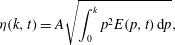 $$\begin{eqnarray}{\it\eta}(k,t)=A\sqrt{\int _{0}^{k}p^{2}E(p,t)\,\text{d}p},\end{eqnarray}$$
following Pouquet et al. (Reference Pouquet, Lesieur, André and Basdevant1975), which is an improved variant of Orszag (Reference Orszag1970)’s proposal. The constant is fixed at
 $A=0.36$
to recover a well-admitted value of the Kolmogorov constant (André & Lesieur Reference André and Lesieur1977). The same equation is used in Weinstock (Reference Weinstock2013). Equation (2.22) can be now integrated using (2.25), (2.24) and (2.26), (2.27), and neglecting the contribution of
 $\unicode[STIX]{x1D613}_{ijn}(\boldsymbol{k},\boldsymbol{p},t)$
. The solution thus obtained involves time integrals that are further simplified by a Markovianization procedure, which amounts to truncating the proper time memory of triple correlations. Even in the isotropic case, the eddy damping allows a posteriori Markovianization to be justified, arguing that the time variation is much more rapid in the exponential eddy-damping term than in the second-order moments present in the quasinormal term. Further details can be found in Cambon et al. (Reference Cambon, Jeandel and Mathieu1981) and Sagaut & Cambon (Reference Sagaut and Cambon2008). In the end, this anisotropic EDQNM closure for the tensor
 ${\it\tau}_{ij}(\boldsymbol{k},t)$
defined by (2.6) amounts to
 $$\begin{eqnarray}{\it\tau}_{ij}(\boldsymbol{k},t)=k_{l}\iiint {\it\theta}_{kpq}\unicode[STIX]{x1D61B}_{ijl}^{(QN)}(\boldsymbol{k},\boldsymbol{p},t)\,\text{d}^{3}\boldsymbol{p},\end{eqnarray}$$
where
 $$\begin{eqnarray}{\it\theta}_{kpq}=\frac{1-\text{e}^{-{\it\mu}_{kpq}t}}{{\it\mu}_{kpq}},\quad {\it\mu}_{kpq}={\it\nu}(k^{2}+p^{2}+q^{2})+{\it\eta}(k,t)+{\it\eta}(p,t)+{\it\eta}(q,t).\end{eqnarray}$$
The expression (2.28) of
 ${\it\tau}_{ij}(\boldsymbol{k},t)$
obtained from the EDQNM approximation is injected into (2.15) and (2.16) in order to obtain closed-form expressions of the transfer terms
 $T^{(\mathscr{E})}(\boldsymbol{k},t)$
and
 $T^{(Z)}(\boldsymbol{k},t)$
:
 $$\begin{eqnarray}\displaystyle T^{(\mathscr{E})}(\boldsymbol{k},t) & = & \displaystyle \iiint {\it\theta}_{kpq}2kp[(\mathscr{E}^{\prime \prime }+\text{Re}\,X^{\prime \prime })[(xy+z^{3})(\mathscr{E}^{\prime }-\mathscr{E})-z(1-z^{2})(\text{Re}\,X^{\prime }-\text{Re}\,X)]\nonumber\\ \displaystyle & & \displaystyle +\,\text{Im}\,X^{\prime \prime }(1-z^{2})(x\,\text{Im}\,X-y\,\text{Im}\,X^{\prime })]\,\text{d}^{3}\boldsymbol{p},\end{eqnarray}$$
 $$\begin{eqnarray}\displaystyle T^{(Z)}(\boldsymbol{k},t)\! & = & \displaystyle \!\iiint {\it\theta}_{kpq}2kp\text{e}^{-2\text{i}{\it\lambda}}[(\mathscr{E}^{\prime \prime }+\text{Re}\,X^{\prime \prime })[\,(xy+z^{3})(\text{Re}\,X^{\prime }-X)-z(1-z^{2})(\mathscr{E}^{\prime }-\mathscr{E})\nonumber\\ \displaystyle & & \displaystyle +\,\text{i}(y^{2}-z^{2})\text{Im}\,X^{\prime }]+\,\text{i}\,\text{Im}\,X^{\prime \prime }(1-z^{2})[x(\mathscr{E}+X)-\text{i}y\,\text{Im}\,X^{\prime }]]\,\text{d}^{3}\boldsymbol{p},\end{eqnarray}$$
with
 $\mathscr{E}=\mathscr{E}(\boldsymbol{k},t)$
,
 $\mathscr{E}^{\prime }=\mathscr{E}(\boldsymbol{p},t)$
,
 $\mathscr{E}^{\prime \prime }=\mathscr{E}(\boldsymbol{q},t)$
,
 $X=Z(\boldsymbol{k},t)\text{e}^{2\text{i}{\it\lambda}}$
,
 $X^{\prime }=Z(\boldsymbol{p},t)\text{e}^{2\text{i}{\it\lambda}^{\prime }}$
,
 $X^{\prime \prime }=Z(\boldsymbol{q},t)\text{e}^{2\text{i}{\it\lambda}^{\prime \prime }}$
,
 $x=-\boldsymbol{p}\boldsymbol{\cdot }\boldsymbol{q}/(pq)$
,
 $y=-\boldsymbol{k}\boldsymbol{\cdot }\boldsymbol{q}/(kq)$
and
 $z=-\boldsymbol{k}\boldsymbol{\cdot }\boldsymbol{p}/(kp)$
. Here,
 ${\it\lambda}$
,
 ${\it\lambda}^{\prime }$
and
 ${\it\lambda}^{\prime \prime }$
are angles that characterize the rotation of the plane of the triad around
 $\boldsymbol{k}$
,
 $\boldsymbol{p}$
and
 $\boldsymbol{q}$
respectively;
 $x$
,
 $y$
and
 $z$
refer to the cosines of the internal angles of the triangle formed by the triad. The above expressions for the transfer terms
 $T^{(\mathscr{E})}(\boldsymbol{k},t)$
and
 $T^{(Z)}(\boldsymbol{k},t)$
are also derived in Cambon et al. (Reference Cambon, Mansour and Godeferd1997) in a different way. Similarly, one can deduce a closed-form expression of the transfer term
 $T^{(RTI)}(\boldsymbol{k},t)$
defined by (2.18), which generates the ‘slow’ component of the pressure–strain rate tensor:
 $$\begin{eqnarray}\displaystyle T^{(RTI)}(\boldsymbol{k},t)\! & = & \displaystyle \!\iiint {\it\theta}_{kpq}2\text{e}^{-\text{i}{\it\lambda}}p(xy+z)\sqrt{1-z^{2}}(\mathscr{E}^{\prime \prime }+\text{Re}\,X^{\prime \prime })\nonumber\\ \displaystyle & & \displaystyle \times \,[(\mathscr{E}+X)(zk-qx)-k(z(\mathscr{E}^{\prime }+\text{Re}\,X^{\prime })-\text{i}\,\text{Im}\,X^{\prime })]\,\text{d}^{3}\boldsymbol{p}.\end{eqnarray}$$
3. Dynamical equations for spherically averaged descriptors
Strictly speaking, the Lin equations (2.12) and (2.13) with the closed-form expressions (2.30) and (2.31) of the transfer terms can be solved. However, important practical difficulties arise from the
 $\boldsymbol{k}$
dependence of the second-order spectral tensor
 $\hat{\unicode[STIX]{x1D619}}_{ij}(\boldsymbol{k},t)$
, or equivalently from those of
 $\mathscr{E}(\boldsymbol{k},t)$
and
 $Z(\boldsymbol{k},t)$
. In order to circumvent these difficulties, one solution is to integrate analytically the closed Lin equations over a sphere of radius
 $k$
. This analytical integration requires a representation of the tensor
 $\hat{\unicode[STIX]{x1D619}}_{ij}(\boldsymbol{k},t)$
, which is described in § 3.1. This representation involves spherically averaged descriptors whose governing equations, which are the main result of this paper, are derived in the remainder of this section. Limitations of the model in terms of anisotropy intensity are quantified in § 3.5.
3.1. Representation of the second-order spectral tensor in terms of spherically averaged descriptors
Here, we use for
 $\hat{\unicode[STIX]{x1D619}}_{ij}(\boldsymbol{k},t)$
the representation proposed by Cambon & Rubinstein (Reference Cambon and Rubinstein2006). This representation involves spherically averaged descriptors and is obtained by treating directionality and polarization anisotropy separately. It is written as
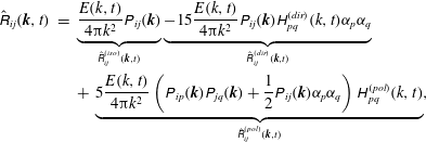 $$\begin{eqnarray}\displaystyle \hat{\unicode[STIX]{x1D619}}_{ij}(\boldsymbol{k},t) & = & \displaystyle \underbrace{\frac{E(k,t)}{4{\rm\pi}k^{2}}\unicode[STIX]{x1D617}_{ij}(\boldsymbol{k})}_{\hat{\unicode[STIX]{x1D619}}_{ij}^{(iso)}(\boldsymbol{k},t)}\underbrace{-15\frac{E(k,t)}{4{\rm\pi}k^{2}}\unicode[STIX]{x1D617}_{ij}(\boldsymbol{k})\unicode[STIX]{x1D60F}_{pq}^{(dir)}(k,t){\it\alpha}_{p}{\it\alpha}_{q}}_{\hat{\unicode[STIX]{x1D619}}_{ij}^{(dir)}(\boldsymbol{k},t)}\nonumber\\ \displaystyle & & \displaystyle +\,\underbrace{5\frac{E(k,t)}{4{\rm\pi}k^{2}}\left(\unicode[STIX]{x1D617}_{ip}(\boldsymbol{k})\unicode[STIX]{x1D617}_{jq}(\boldsymbol{k})+\frac{1}{2}\unicode[STIX]{x1D617}_{ij}(\boldsymbol{k}){\it\alpha}_{p}{\it\alpha}_{q}\right)\unicode[STIX]{x1D60F}_{pq}^{(pol)}(k,t)}_{\hat{\unicode[STIX]{x1D619}}_{ij}^{(pol)}(\boldsymbol{k},t)},\end{eqnarray}$$
or equivalently
 $$\begin{eqnarray}\mathscr{E}(\boldsymbol{k},t)=\frac{E(k,t)}{4{\rm\pi}k^{2}}(1-15\unicode[STIX]{x1D60F}_{ij}^{(dir)}(k,t){\it\alpha}_{i}{\it\alpha}_{j}),\quad Z(\boldsymbol{k},t)=\frac{5}{2}\frac{E(k,t)}{4{\rm\pi}k^{2}}\unicode[STIX]{x1D60F}_{ij}^{(pol)}(k,t)N_{i}^{\ast }(\boldsymbol{k})N_{j}^{\ast }(\boldsymbol{k}),\end{eqnarray}$$
where the tensor
 $\unicode[STIX]{x1D617}_{ij}(\boldsymbol{k})$
is defined in (1.1) and
 ${\it\alpha}_{i}=k_{i}/k$
. The tensors
 $\hat{\unicode[STIX]{x1D619}}_{ij}^{(iso)}(\boldsymbol{k},t)$
,
 $\hat{\unicode[STIX]{x1D619}}_{ij}^{(dir)}(\boldsymbol{k},t)$
and
 $\hat{\unicode[STIX]{x1D619}}_{ij}^{(pol)}(\boldsymbol{k},t)$
identify the isotropic, directional and polarization parts of
 $\hat{\unicode[STIX]{x1D619}}_{ij}(\boldsymbol{k},t)$
respectively. The representation (3.1) is constructed so that the trace-free tensors
 $\unicode[STIX]{x1D60F}_{ij}^{(dir)}(k,t)$
and
 $\unicode[STIX]{x1D60F}_{ij}^{(pol)}(k,t)$
, which depend only on
 $k$
, measure the directional anisotropy and polarization anisotropy according to (1.5). Injecting the representation of
 $\mathscr{E}(\boldsymbol{k},t)$
and
 $Z(\boldsymbol{k},t)$
(3.2) into (2.12) and (2.13) and (2.30) and (2.31) allows us to integrate the latter analytically over a sphere of radius
 $k$
and to derive a system of governing equations in terms of the spherically averaged descriptors
 $E(k,t)$
,
 $\unicode[STIX]{x1D60F}_{ij}^{(dir)}(k,t)$
and
 $\unicode[STIX]{x1D60F}_{ij}^{(pol)}(k,t)$
. In view of (3.1), (3.2) and (1.4), the latter completely determine the second-order spectral tensor
 $\hat{\unicode[STIX]{x1D619}}_{ij}(\boldsymbol{k},t)$
and its spherically integrated counterpart
 ${\it\varphi}_{ij}(k,t)$
, however restricted to moderate anisotropy. This point is discussed in § 3.5.
3.2. Dynamics, final closure
The system of governing equations for the spherically averaged descriptors
 $E(k,t)$
,
 $\unicode[STIX]{x1D60F}_{ij}^{(dir)}(k,t)$
and
 $\unicode[STIX]{x1D60F}_{ij}^{(pol)}(k,t)$
, which is the main result of this article, is written as follows:
 $$\begin{eqnarray}\displaystyle & \displaystyle \left(\frac{\partial }{\partial t}+2{\it\nu}k^{2}\right)E(k,t)=S^{L}(k,t)+T(k,t), & \displaystyle\end{eqnarray}$$
 $$\begin{eqnarray}\displaystyle & \displaystyle \left(\frac{\partial }{\partial t}+2{\it\nu}k^{2}\right)E(k,t)\unicode[STIX]{x1D60F}_{ij}^{(dir)}(k,t)=\unicode[STIX]{x1D61A}_{ij}^{L(dir)}(k,t)+\unicode[STIX]{x1D61A}_{ij}^{NL(dir)}(k,t), & \displaystyle\end{eqnarray}$$
 $$\begin{eqnarray}\displaystyle & \displaystyle \left(\frac{\partial }{\partial t}+2{\it\nu}k^{2}\right)E(k,t)\unicode[STIX]{x1D60F}_{ij}^{(pol)}(k,t)=\unicode[STIX]{x1D61A}_{ij}^{L(pol)}(k,t)+\unicode[STIX]{x1D61A}_{ij}^{NL(pol)}(k,t), & \displaystyle\end{eqnarray}$$
 $$\begin{eqnarray}2\left(\frac{{\it\delta}_{ij}}{3}T(k,t)+\unicode[STIX]{x1D61A}_{ij}^{NL(dir)}(k,t)+\unicode[STIX]{x1D61A}_{ij}^{NL(pol)}(k,t)\right)=\unicode[STIX]{x1D61A}_{ij}(k,t)+\unicode[STIX]{x1D617}_{ij}(k,t).\end{eqnarray}$$
The tensors
 $S^{L}(k,t)$
,
 $\unicode[STIX]{x1D61A}_{ij}^{L(dir)}(k,t)$
and
 $\unicode[STIX]{x1D61A}_{ij}^{L(pol)}(k,t)$
account for the linear terms corresponding to the interactions with the mean flow, whereas
 $T(k,t)$
,
 $\unicode[STIX]{x1D61A}_{ij}^{NL(dir)}(k,t)$
and
 $\unicode[STIX]{x1D61A}_{ij}^{NL(pol)}(k,t)$
correspond to nonlinear transfer terms. The tensor
 $\unicode[STIX]{x1D617}_{ij}(k,t)$
is the spherically integrated spectral counterpart of the slow pressure–strain rate tensor, to which an RTI is conventionally attributed. The tensor
 $\unicode[STIX]{x1D61A}_{ij}(k,t)$
corresponds to a ‘true’ transfer tensor with
 $\int _{0}^{\infty }\unicode[STIX]{x1D61A}_{ij}(k,t)\,\text{d}k=0\;\forall t$
. Since the tensors
 $\unicode[STIX]{x1D60F}_{ij}^{(dir)}(k,t)$
and
 $\unicode[STIX]{x1D60F}_{ij}^{(pol)}(k,t)$
are symmetric and trace-free, the system (3.3)–(3.5) forms a set of 11 independent equations.
3.3. Closure for the linear terms induced by mean-gradient effects
These terms are exact and linear in the equation governing the full spectral tensor, or equivalently
 $\mathscr{E}(\boldsymbol{k},t)$
and
 $Z(\boldsymbol{k},t)$
. Taken independently with zero contribution from third-order correlations, they reflect the RDT limit for the evolution of two-point second-order velocity correlations. In order to obtain the corresponding spherically averaged terms
 $S^{L}(k,t)$
,
 $\unicode[STIX]{x1D61A}_{ij}^{L(dir)}(k,t)$
and
 $\unicode[STIX]{x1D61A}_{ij}^{L(pol)}(k,t)$
, one has to analytically solve the spherical averaging of tensorial products of vectors
 ${\bf\alpha}=\boldsymbol{k}/k$
. This is done following the procedure described in Cambon et al. (Reference Cambon, Jeandel and Mathieu1981). Performing the spherical integration of the linear terms in (2.3) or that of the linear terms in (2.12), (2.13) with the representation (3.1) or (3.2) leads to
 $$\begin{eqnarray}S^{L}(k,t)=-2\unicode[STIX]{x1D61A}_{lm}\frac{\partial }{\partial k}(kE\unicode[STIX]{x1D60F}_{lm}^{(dir)})-2E\unicode[STIX]{x1D61A}_{lm}\left(\unicode[STIX]{x1D60F}_{lm}^{(dir)}+\unicode[STIX]{x1D60F}_{lm}^{(pol)}\right),\end{eqnarray}$$
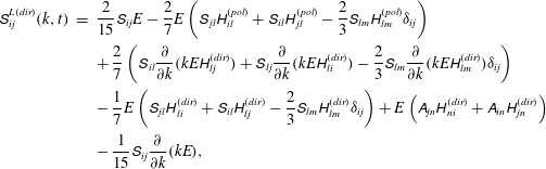 $$\begin{eqnarray}\displaystyle \unicode[STIX]{x1D61A}_{ij}^{L(dir)}(k,t) & = & \displaystyle \frac{2}{15}\unicode[STIX]{x1D61A}_{ij}E-\frac{2}{7}E\left(\unicode[STIX]{x1D61A}_{jl}\unicode[STIX]{x1D60F}_{il}^{(pol)}+\unicode[STIX]{x1D61A}_{il}\unicode[STIX]{x1D60F}_{jl}^{(pol)}-\frac{2}{3}\unicode[STIX]{x1D61A}_{lm}\unicode[STIX]{x1D60F}_{lm}^{(pol)}{\it\delta}_{ij}\right)\nonumber\\ \displaystyle & & \displaystyle +\,\frac{2}{7}\left(\unicode[STIX]{x1D61A}_{il}\frac{\partial }{\partial k}(kE\unicode[STIX]{x1D60F}_{lj}^{(dir)})+\unicode[STIX]{x1D61A}_{lj}\frac{\partial }{\partial k}(kE\unicode[STIX]{x1D60F}_{li}^{(dir)})-\frac{2}{3}\unicode[STIX]{x1D61A}_{lm}\frac{\partial }{\partial k}(kE\unicode[STIX]{x1D60F}_{lm}^{(dir)}){\it\delta}_{ij}\right)\nonumber\\ \displaystyle & & \displaystyle -\,\frac{1}{7}E\left(\unicode[STIX]{x1D61A}_{jl}\unicode[STIX]{x1D60F}_{li}^{(dir)}+\unicode[STIX]{x1D61A}_{il}\unicode[STIX]{x1D60F}_{lj}^{(dir)}-\frac{2}{3}\unicode[STIX]{x1D61A}_{lm}\unicode[STIX]{x1D60F}_{lm}^{(dir)}{\it\delta}_{ij}\right)+E\left(\unicode[STIX]{x1D608}_{jn}\unicode[STIX]{x1D60F}_{ni}^{(dir)}+\unicode[STIX]{x1D608}_{in}\unicode[STIX]{x1D60F}_{jn}^{(dir)}\right)\nonumber\\ \displaystyle & & \displaystyle -\,\frac{1}{15}\unicode[STIX]{x1D61A}_{ij}\frac{\partial }{\partial k}(kE),\end{eqnarray}$$
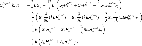 $$\begin{eqnarray}\displaystyle \unicode[STIX]{x1D61A}_{ij}^{L(pol)}(k,t) & = & \displaystyle -\frac{2}{5}E\unicode[STIX]{x1D61A}_{ij}-\frac{12}{7}E\left(\unicode[STIX]{x1D61A}_{lj}\unicode[STIX]{x1D60F}_{li}^{(dir)}+\unicode[STIX]{x1D61A}_{il}\unicode[STIX]{x1D60F}_{lj}^{(dir)}-\frac{2}{3}\unicode[STIX]{x1D61A}_{lm}\unicode[STIX]{x1D60F}_{lm}^{(dir)}{\it\delta}_{ij}\right)\nonumber\\ \displaystyle & & \displaystyle -\,\frac{2}{7}\left(\unicode[STIX]{x1D61A}_{jl}\frac{\partial }{\partial k}(kE\unicode[STIX]{x1D60F}_{il}^{(pol)})+\unicode[STIX]{x1D61A}_{il}\frac{\partial }{\partial k}(kE\unicode[STIX]{x1D60F}_{lj}^{(pol)})-\frac{2}{3}\unicode[STIX]{x1D61A}_{ln}\frac{\partial }{\partial k}(kE\unicode[STIX]{x1D60F}_{ln}^{(pol)}){\it\delta}_{ij}\right)\nonumber\\ \displaystyle & & \displaystyle +\,\frac{1}{7}E\left(\unicode[STIX]{x1D61A}_{il}\unicode[STIX]{x1D60F}_{lj}^{(pol)}+\unicode[STIX]{x1D61A}_{jl}\unicode[STIX]{x1D60F}_{li}^{(pol)}-\frac{2}{3}\unicode[STIX]{x1D61A}_{lm}\unicode[STIX]{x1D60F}_{lm}^{(pol)}{\it\delta}_{ij}\right)\nonumber\\ \displaystyle & & \displaystyle -\,\frac{1}{3}E\left(\unicode[STIX]{x1D608}_{il}\unicode[STIX]{x1D60F}_{lj}^{(pol)}+\unicode[STIX]{x1D608}_{jl}\unicode[STIX]{x1D60F}_{li}^{(pol)}\right),\end{eqnarray}$$
with
 $E=E(k,t)$
,
 $\unicode[STIX]{x1D60F}_{ij}^{(dir)}=\unicode[STIX]{x1D60F}_{ij}^{(dir)}(k,t)$
,
 $\unicode[STIX]{x1D60F}_{ij}^{(pol)}=\unicode[STIX]{x1D60F}_{ij}^{(pol)}(k,t)$
,
 $\unicode[STIX]{x1D61A}_{ij}=({\it\lambda}_{ij}+{\it\lambda}_{ji})/2$
,
 $\unicode[STIX]{x1D608}_{ij}=({\it\lambda}_{ij}-{\it\lambda}_{ji})/2$
;
 ${\it\lambda}_{ij}$
refers to the mean-flow gradient as previously stated.
3.4. Closure for the terms mediated by third-order correlations
The transfer terms
 $T(k,t)$
,
 $\unicode[STIX]{x1D61A}_{ij}^{NL(dir)}(k,t)$
and
 $\unicode[STIX]{x1D61A}_{ij}^{NL(pol)}(k,t)$
are obtained from the spherical integration of the expressions of the transfer terms
 $T^{(\mathscr{E})}(\boldsymbol{k},t)$
and
 $T^{(Z)}(\boldsymbol{k},t)$
closed by the EDQNM procedure (2.30) and (2.31) and using the representation (3.2) for
 $\mathscr{E}(\boldsymbol{k},t)$
and
 $Z(\boldsymbol{k},t)$
. It is consistent to retain only linear contributions from the tensors
 $\unicode[STIX]{x1D60F}_{ij}^{(dir)}(k,t)$
and
 $\unicode[STIX]{x1D60F}_{ij}^{(pol)}(k,t)$
in the terms present on the right-hand sides of the system (3.3)–(3.5) in view of the discussion in § 3.5. Their low contribution is checked in § 4.7. In anisotropic triadic closure, the new difficulty is to solve the integral over the orientation of the plane of the triad (Cambon et al.
Reference Cambon, Mansour and Godeferd1997; Sagaut & Cambon Reference Sagaut and Cambon2008), which is performed analytically. The final results are
 $$\begin{eqnarray}T(k,t)=\iint _{{\it\Delta}_{k}}{\it\theta}_{kpq}16{\rm\pi}^{2}p^{2}k^{2}q(xy+z^{3})\mathscr{E}_{0}^{\prime \prime }(\mathscr{E}_{0}^{\prime }-\mathscr{E}_{0})\,\text{d}p\,\text{d}q,\end{eqnarray}$$
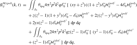
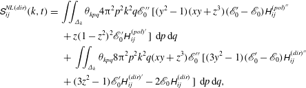 $$\begin{eqnarray}\displaystyle \unicode[STIX]{x1D61A}_{ij}^{NL(dir)}(k,t)\! & = & \displaystyle \!\iint _{{\it\Delta}_{k}}{\it\theta}_{kpq}4{\rm\pi}^{2}p^{2}k^{2}q\mathscr{E}_{0}^{\prime \prime }[(y^{2}-1)(xy+z^{3})(\mathscr{E}_{0}^{\prime }-\mathscr{E}_{0})\unicode[STIX]{x1D60F}_{ij}^{(pol)^{\prime \prime }}\nonumber\\ \displaystyle & & \displaystyle +\,z(1-z^{2})^{2}\mathscr{E}_{0}^{\prime }\unicode[STIX]{x1D60F}_{ij}^{(pol)^{\prime }}]\,\text{d}p\,\text{d}q\nonumber\\ \displaystyle & & \displaystyle +\,\iint _{{\it\Delta}_{k}}{\it\theta}_{kpq}8{\rm\pi}^{2}p^{2}k^{2}q(xy+z^{3})\mathscr{E}_{0}^{\prime \prime }[(3y^{2}-1)(\mathscr{E}_{0}^{\prime }-\mathscr{E}_{0})\unicode[STIX]{x1D60F}_{ij}^{(dir)^{\prime \prime }}\nonumber\\ \displaystyle & & \displaystyle +\,(3z^{2}-1)\mathscr{E}_{0}^{\prime }\unicode[STIX]{x1D60F}_{ij}^{(dir)^{\prime }}-2\mathscr{E}_{0}\unicode[STIX]{x1D60F}_{ij}^{(dir)} ]\,\text{d}p\,\text{d}q,\end{eqnarray}$$
 $$\begin{eqnarray}\displaystyle \unicode[STIX]{x1D61A}_{ij}^{NL(pol)}(k,t) & = & \displaystyle \iint _{{\it\Delta}_{k}}{\it\theta}_{kpq}4{\rm\pi}^{2}p^{2}k^{2}q\mathscr{E}_{0}^{\prime \prime }[\,(xy+z^{3})((1+z^{2})\mathscr{E}_{0}^{\prime }\unicode[STIX]{x1D60F}_{ij}^{(pol)^{\prime }}-4\mathscr{E}_{0}\unicode[STIX]{x1D60F}_{ij}^{(pol)})\nonumber\\ \displaystyle & & \displaystyle +\,z(z^{2}-1)(1+y^{2})(\mathscr{E}_{0}^{\prime }-\mathscr{E}_{0})\unicode[STIX]{x1D60F}_{ij}^{(pol)^{\prime \prime }}+2z(z^{2}-y^{2})\mathscr{E}_{0}^{\prime }\unicode[STIX]{x1D60F}_{ij}^{(pol)^{\prime }}\nonumber\\ \displaystyle & & \displaystyle +\,2yx(z^{2}-1)\mathscr{E}_{0}\unicode[STIX]{x1D60F}_{ij}^{(pol)^{\prime \prime }}]\,\text{d}p\,\text{d}q\nonumber\\ \displaystyle & & \displaystyle +\,\iint _{{\it\Delta}_{k}}{\it\theta}_{kpq}24{\rm\pi}^{2}p^{2}k^{2}qz(z^{2}-1)\mathscr{E}_{0}^{\prime \prime }[\,(y^{2}-1)(\mathscr{E}_{0}^{\prime }-\mathscr{E}_{0})\unicode[STIX]{x1D60F}_{ij}^{(dir)^{\prime \prime }}\nonumber\\ \displaystyle & & \displaystyle +\,(z^{2}-1)\mathscr{E}_{0}^{\prime }\unicode[STIX]{x1D60F}_{ij}^{(dir)^{\prime }}]\,\text{d}p\,\text{d}q,\end{eqnarray}$$
 $$\begin{eqnarray}\displaystyle \unicode[STIX]{x1D617}_{ij}(k,t) & = & \displaystyle \iint _{{\it\Delta}_{k}}{\it\theta}_{kpq}16{\rm\pi}^{2}p^{2}k^{2}q(yz+x)\mathscr{E}_{0}^{\prime \prime }[\mathscr{E}_{0}^{\prime }(y(z^{2}-y^{2})(6\unicode[STIX]{x1D60F}_{ij}^{(dir)^{\prime \prime }}+\unicode[STIX]{x1D60F}_{ij}^{(pol)^{\prime \prime }})\nonumber\\ \displaystyle & & \displaystyle -\,(xz+y)\unicode[STIX]{x1D60F}_{ij}^{(pol)^{\prime \prime }})-y(z^{2}-x^{2})\mathscr{E}_{0}(6\unicode[STIX]{x1D60F}_{ij}^{(dir)^{\prime \prime }}+\unicode[STIX]{x1D60F}_{ij}^{(pol)^{\prime \prime }})]\,\text{d}p\,\text{d}q,\end{eqnarray}$$
with
 $\mathscr{E}_{0}=(E(k,t))/(4{\rm\pi}k^{2})$
,
 $\mathscr{E}_{0}^{\prime }=(E(p,t))/(4{\rm\pi}p^{2})$
,
 $\mathscr{E}_{0}^{\prime \prime }=(E(q,t))/(4{\rm\pi}q^{2})$
,
 $\unicode[STIX]{x1D60F}_{ij}^{()}=\unicode[STIX]{x1D60F}_{ij}^{()}(k,t)$
,
 $\unicode[STIX]{x1D60F}_{ij}^{()^{\prime }}=\unicode[STIX]{x1D60F}_{ij}^{()}(p,t)$
and
 $\unicode[STIX]{x1D60F}_{ij}^{()^{\prime \prime }}=\unicode[STIX]{x1D60F}_{ij}^{()}(q,t)$
, where
 $\unicode[STIX]{x1D60F}_{ij}^{()}$
may refer to either
 $\unicode[STIX]{x1D60F}_{ij}^{(dir)}$
or
 $\unicode[STIX]{x1D60F}_{ij}^{(pol)}$
. The integrals over
 $p$
and
 $q$
are performed over the domain
 ${\it\Delta}_{k}$
, so that
 $k$
,
 $p$
and
 $q$
are the lengths of the sides of the triangle formed by
 $\boldsymbol{k}$
,
 $\boldsymbol{p}$
and
 $\boldsymbol{q}$
. The expression of the ‘true’ transfer
 $\unicode[STIX]{x1D61A}_{ij}(k,t)$
can be deduced from (3.6) and (3.10)–(3.13).
3.5. Properties of the model
Spherical averaging of the Lin equations (2.12)–(2.13) allows us to obtain a model for anisotropic turbulence that can be used to calculate anisotropic turbulent flows at both very high and low Reynolds numbers, with good resolution of both large and small scales and over very long evolution times. Besides, (3.3)–(3.5) remain consistent with the decomposition of
 $\hat{\unicode[STIX]{x1D64D}}(\boldsymbol{k},t)$
in terms of directional anisotropy and polarization anisotropy. However, spherical integration also has a drawback since it implies a loss of information, which restricts the present model to moderately anisotropic flows. Looking at expansions of the scalars
 $\mathscr{E}(\boldsymbol{k},t)$
and
 $Z(\boldsymbol{k},t)$
in terms of powers of
 ${\bf\alpha}=\boldsymbol{k}/k$
, the first approach by Cambon & Rubinstein (Reference Cambon and Rubinstein2006) can be translated into the following:
 $$\begin{eqnarray}\displaystyle & \hspace{-20.00003pt}\mathscr{E}(\boldsymbol{k},t)=\displaystyle \frac{E(k,t)}{4{\rm\pi}k^{2}}\left(1+\unicode[STIX]{x1D61C}_{ij}^{(dir)2}(k,t){\it\alpha}_{i}{\it\alpha}_{j}+\unicode[STIX]{x1D61C}_{ijmn}^{(dir)4}(k,t){\it\alpha}_{i}{\it\alpha}_{j}{\it\alpha}_{m}{\it\alpha}_{n}+\cdots \!\right), & \displaystyle\end{eqnarray}$$
 $$\begin{eqnarray}\displaystyle & \hspace{-20.00003pt}\displaystyle Z(\boldsymbol{k},t)=\frac{1}{2}\frac{E(k,t)}{4{\rm\pi}k^{2}}\left(\unicode[STIX]{x1D61C}_{ij}^{(pol)2}(k,t)+\unicode[STIX]{x1D61C}_{ijm}^{(pol)3}(k,t){\it\alpha}_{m}+\unicode[STIX]{x1D61C}_{ijmn}^{(pol)4}(k,t){\it\alpha}_{m}{\it\alpha}_{n}+\cdots \!\right)N_{i}^{\ast }(\boldsymbol{k})N_{j}^{\ast }(\boldsymbol{k}). & \displaystyle \nonumber\\ \displaystyle & & \displaystyle\end{eqnarray}$$
The latter form is consistent with both scalar (for (3.14)) and tensor (for (3.15)) spherical harmonic expansion generated by the rotation group SO
 $^{3}$
decomposition, in agreement with Rubinstein, Kurien & Cambon (Reference Rubinstein, Kurien and Cambon2015). With the identification
 $$\begin{eqnarray}\unicode[STIX]{x1D61C}_{ij}^{(dir)2}(k,t)=-15\unicode[STIX]{x1D60F}_{ij}^{(dir)}(k,t),\quad \unicode[STIX]{x1D61C}_{ij}^{(pol)2}(k,t)=5\unicode[STIX]{x1D60F}_{ij}^{(pol)}(k,t),\end{eqnarray}$$
the representation (3.2) is interpreted as the first-order truncation of expansions (3.14) and (3.15). The truncation of (3.14) and (3.15) lies at the origin of the loss of information, which limits the degree of anisotropy that can be investigated with the present model. The degree of anisotropy permitted by the representation (3.1) can be derived from realizability conditions. One may use condition (2.11). In order to derive a simple condition in terms of the tensors
 $\unicode[STIX]{x1D60F}_{ij}^{(dir)}(k,t)$
and
 $\unicode[STIX]{x1D60F}_{ij}^{(pol)}(k,t)$
, one may also consider the weaker condition
 $\mathscr{E}(\boldsymbol{k},t)\geqslant 0\;\forall \boldsymbol{k},t$
, which already proves to be very restrictive. In view of (3.2), this condition is equivalent to
 $$\begin{eqnarray}\max _{i}{\it\Lambda}_{i}(\unicode[STIX]{x1D60F}^{(dir)}(k,t))\leqslant {\textstyle \frac{1}{15}}\;\forall k,t,\end{eqnarray}$$
where
 ${\it\Lambda}_{i}(\unicode[STIX]{x1D60F}^{(dir)}(k,t))$
refers to the eigenvalues of
 $\unicode[STIX]{x1D60F}_{ij}^{(dir)}(k,t)$
. Condition (3.17) can help to quantify the upper boundary of anisotropy intensity to ensure that the present model represents correctly the corresponding turbulent flow. In § 4.7, criterion (3.17) is computed for the different flow configurations studied in this paper in order to check whether the representation (3.2) and the governing equations (3.3)–(3.5) can describe the corresponding turbulent flow. Since the representation (3.2) is restricted to the description of moderate anisotropy, we discard quadratic contributions from the tensors
 $\unicode[STIX]{x1D60F}_{ij}^{(dir)}(k,t)$
and
 $\unicode[STIX]{x1D60F}_{ij}^{(pol)}(k,t)$
which appear when the representation (3.2) is injected into (2.30)–(2.32). It is also important to keep in mind that the nonlinear transfer terms of the system (3.3)–(3.5) are not relevant when the mean flow acts only on triple correlations such as in the case for solid-body rotation, but are restricted to mean flows leading to linear production effects in the equations for second-order correlations. This is due to the specific EDQNM version used in § 2.4. In the end, the present model is suited for the study of turbulent flows where the anisotropy is moderate and where linear effects induced by mean-velocity gradients play a negligible role in the dynamics of triple correlations compared with those directly induced in the equations for second-order correlations. Since only flows dominated by production effects induced by a mean strain or shear are considered in § 4, we expect the EDQNM closure of § 2.4 to be valid in these configurations. Besides, the linear contributions in (3.4) and (3.5) originate from the exact linear terms of (2.12) and (2.13). Accordingly, it is inferred that the main source of possible discrepancies between the predictions obtained with (3.3)–(3.5) and experimental/direct numerical simulation (DNS) results is due to the loss of information following the first-order truncation of (3.14) and (3.15).
4. First applications and results: RTI and effect of mean shear
4.1. Physical and numerical set-up
The predictions of the model presented in § 3 are first compared with data from the experiments of Gence & Mathieu (Reference Gence and Mathieu1979, Reference Gence and Mathieu1980). In these studies, two successive plane strains with different orientations are applied to grid-generated turbulence, and the RTI of the turbulence thus obtained is investigated in the latter experiment. We then consider the experiment of Chen, Meneveau & Katz (Reference Chen, Meneveau and Katz2006), where turbulence is subjected to a non-stationary straining–relaxation–destraining cycle. Both linear and nonlinear phenomena come into play in the response of turbulence to this particular straining. The case of turbulence subjected to an axisymmetric expansion or contraction is then investigated. The set-up of the numerical simulations performed with the present model is similar to that of the DNS of Zusi & Perot (Reference Zusi and Perot2014). In particular, we want to check the ability of the present model to capture the initial increase of anisotropy when the strain is removed, only in the case of axisymmetric expansion, which is observed in the above-mentioned study. The next test case deals with an initially isotropic flow which is suddenly subjected to a mean shear and is then released. A comparison with the use of RDT to initialize the anisotropy of the flow will allow us to validate the linear part of the present model in the case of homogeneous shear turbulence. This case will also allow us to confirm the consistency between the present model and the permanence of large eddies (PLE). Finally, we consider the case where the mean shear is maintained during the evolution of the flow. Homogeneous shear turbulence has been studied experimentally (Tavoularis & Corrsin Reference Tavoularis and Corrsin1981; Tavoularis Reference Tavoularis1985; Rohr et al. Reference Rohr, Itsweire, Helland and Van Atta1988; Tavoularis & Karnik Reference Tavoularis and Karnik1989; Shen & Warhaft Reference Shen and Warhaft2000), numerically (Rogers, Moin & Reynolds Reference Rogers, Moin and Reynolds1986; Ishihara, Yoshida & Kaneda Reference Ishihara, Yoshida and Kaneda2002; Brethouwer Reference Brethouwer2005; Isaza & Collins Reference Isaza and Collins2009) and theoretically (Lumley Reference Lumley1967; Leslie Reference Leslie1973; Yoshida et al. Reference Yoshida, Ishihara and Kaneda2003; Weinstock Reference Weinstock2013), and the results obtained with the system (3.3)–(3.5) will be compared with the predictions of these different studies. In the last subsection, it is checked that condition (3.17) is verified for all of the flow configurations discussed above.
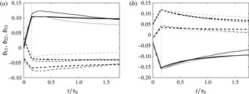
As briefly mentioned above, concerning the study of the RTI of shear-released turbulence, the anisotropy of the flow can be initialized in two ways. A first possibility consists in deriving analytically an initial anisotropic condition thanks to RDT. The other option is to start with an isotropic field and to generate the anisotropy with the linear terms of (3.3)–(3.5) that account for the interactions with a mean flow. For
 $St\ll 1$
, where
 $S$
refers to the characteristic shear rate, these two ways of introducing anisotropy must be equivalent. This will help to validate the model developed in this paper. The complete RDT solution for homogeneous shear turbulence can be found in Townsend (Reference Townsend1976), Piquet (Reference Piquet2001) and Sagaut & Cambon (Reference Sagaut and Cambon2008). The energy spectrum used for the RDT calculations, or directly to initialize the simulations, is written as
 $$\begin{eqnarray}E(k)=C{\it\varepsilon}^{2/3}k^{-(5/3)}f(kL)g(k{\it\eta}),\end{eqnarray}$$
with
 $$\begin{eqnarray}f(x)=\left(\frac{x}{\displaystyle \left(x^{1.5}+1.5-\frac{{\it\sigma}}{4}\right)^{1/1.5}}\right)^{(5/3)+{\it\sigma}},\quad g(x)=\exp (-5.2((x^{4}+0.4^{4})^{1/4}-0.4)).\end{eqnarray}$$
The functions defined by (4.2) have been proposed by Pope (Reference Pope2000) and Meyers & Meneveau (Reference Meyers and Meneveau2008) respectively. Here,
 ${\it\varepsilon}$
refers to the dissipation rate,
 $L$
to the integral length scale,
 ${\it\eta}$
to the Kolmogorov scale, and
 ${\it\sigma}$
is the slope at large scales of the energy spectrum (
 $E(k\rightarrow 0)\propto k^{{\it\sigma}}$
). In all simulations we set
 ${\it\sigma}=2$
, which corresponds to Saffman turbulence. The integral scale
 $L$
and the Reynolds number are prescribed at the beginning of the simulation. As a consequence,
 ${\it\eta}$
is initialized thanks to the relation
 ${\it\eta}=((3/20)Re_{{\it\lambda}}^{2})^{-(3/4)}L$
, where
 $Re_{{\it\lambda}}$
is the Reynolds number based on the Taylor microscale
 ${\it\lambda}=\sqrt{10\mathscr{K}{\it\nu}/{\it\varepsilon}}$
. The constant
 $C$
in (4.1) is adjusted in order to impose the initial value of the turbulent kinetic energy
 $\mathscr{K}$
so that
 $\mathscr{K}(t=0)/\tilde{\mathscr{K}}_{0}=1$
, where
 $\tilde{\mathscr{K}}_{0}$
is a reference energy. The spectral mesh used to perform the simulations covers a very broad wavenumber range in the spectral domain. The smallest wavenumber of the mesh
 $k_{0}$
(which roughly corresponds to the largest resolved scale) is chosen so that
 $k_{0}=10^{-8}k_{L}(t=0)$
, where
 $k_{L}=1/L$
is the wavenumber associated with the integral length scale
 $L$
. The largest resolved wavenumber
 $k_{N}$
is chosen such that a resolution of at least one decade at small scales, with respect to the initial value of the Kolmogorov scale
 ${\it\eta}(t=0)$
, is granted. The relation
 $k_{N}=10k_{{\it\eta}}(0)$
is thus imposed, where
 $k_{{\it\eta}}=1/{\it\eta}$
. The total number of elements
 $N+1$
is recovered so that
 $k_{N}=r^{N}k_{0}$
, where
 $r$
represents the constant aspect ratio between contiguous elements of the mesh. In the present work,
 $r=1.122$
, which means that each decade in the spectral space is discretized by
 $20$
mesh elements. The temporal integration is made by a forward Euler scheme, and the Courant–Friedrichs–Lewy condition is based on the Kolmogorov scale (Lesieur Reference Lesieur2008).
The anisotropy at the spectral level is evaluated with the deviatoric tensors
 $\unicode[STIX]{x1D60F}_{ij}^{(dir)}(k,t)$
and
 $\unicode[STIX]{x1D60F}_{ij}^{(pol)}(k,t)$
introduced in § 3.1, and
 $\unicode[STIX]{x1D60F}_{ij}(k,t)=\unicode[STIX]{x1D60F}_{ij}^{(dir)}(k,t)+\unicode[STIX]{x1D60F}_{ij}^{(pol)}(k,t)$
. The global anisotropy is quantified via the tensors
 $\unicode[STIX]{x1D623}_{ij}^{(dir)}(t)$
,
 $\unicode[STIX]{x1D623}_{ij}^{(pol)}(t)$
and
 $\unicode[STIX]{x1D623}_{ij}(t)=\unicode[STIX]{x1D623}_{ij}^{(dir)}(t)+\unicode[STIX]{x1D623}_{ij}^{(pol)}(t)$
, which originate from the
 $(\mathscr{E},Z)$
decomposition of the Reynolds stress tensor:
 $$\begin{eqnarray}\langle u_{i}u_{j}\rangle (t)=2\unicode[STIX]{x1D612}_{ij}(t)=2\mathscr{K}(t)\left(\frac{{\it\delta}_{ij}}{3}+\unicode[STIX]{x1D623}_{ij}^{(dir)}(t)+\unicode[STIX]{x1D623}_{ij}^{(pol)}(t)\right),\quad \mathscr{K}(t)=\unicode[STIX]{x1D612}_{ii}(t).\end{eqnarray}$$
The tensors
 $\unicode[STIX]{x1D623}_{ij}^{(dir)}(t)$
and
 $\unicode[STIX]{x1D623}_{ij}^{(pol)}(t)$
are calculated from the tensors
 $\unicode[STIX]{x1D60F}_{ij}^{(dir)}(k,t)$
and
 $\unicode[STIX]{x1D60F}_{ij}^{(pol)}(k,t)$
according to
 $$\begin{eqnarray}\unicode[STIX]{x1D623}_{ij}^{(dir)}(t)=\int _{0}^{\infty }E(k,t)\unicode[STIX]{x1D60F}_{ij}^{(dir)}(k,t)\,\text{d}k/\mathscr{K}(t),\quad \unicode[STIX]{x1D623}_{ij}^{(pol)}(t)=\int _{0}^{\infty }E(k,t)\unicode[STIX]{x1D60F}_{ij}^{(pol)}(k,t)\,\text{d}k/\mathscr{K}(t).\end{eqnarray}$$
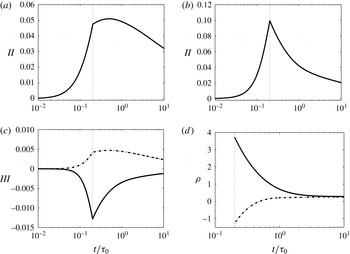
We define the invariants
 $\mathit{II}(t)$
and
 $\mathit{III}(t)$
as
 $$\begin{eqnarray}\mathit{II}(t)=\unicode[STIX]{x1D623}_{ij}(t)\unicode[STIX]{x1D623}_{ji}(t),\quad \mathit{III}(t)=\unicode[STIX]{x1D623}_{ik}(t)\unicode[STIX]{x1D623}_{kj}(t)\unicode[STIX]{x1D623}_{ij}(t).\end{eqnarray}$$
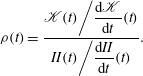
In order to quantitatively characterize the RTI process, we introduce the ratio
 ${\it\rho}(t)$
between a characteristic time of turbulence decay and a characteristic time of RTI, namely
 $$\begin{eqnarray}{\it\rho}(t)=\frac{\displaystyle \mathscr{K}(t)\bigg/\displaystyle \frac{\text{d}\mathscr{K}}{\text{d}t}(t)}{\displaystyle \mathit{II}(t)\bigg/\displaystyle \frac{\text{d}\mathit{II}}{\text{d}t}(t)}.\end{eqnarray}$$
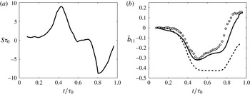
For the comparison with the experiment of Chen et al. (Reference Chen, Meneveau and Katz2006), we use a two-component surrogate of the anisotropic tensor
 $\unicode[STIX]{x1D623}_{ij}(t)$
, defined as
 $$\begin{eqnarray}\tilde{\unicode[STIX]{x1D623}}_{ij}(t)=\frac{\unicode[STIX]{x1D612}_{ij}(t)/\unicode[STIX]{x1D612}_{ij}(t_{0})}{\unicode[STIX]{x1D612}_{11}(t)/\unicode[STIX]{x1D612}_{11}(t_{0})+\unicode[STIX]{x1D612}_{22}(t)/\unicode[STIX]{x1D612}_{22}(t_{0})}-\frac{1}{2}{\it\delta}_{ij}\quad (i,j=1,2),\end{eqnarray}$$
where
 $t_{0}$
refers to the time at which strain starts. The budget terms of the governing equation for the spherically integrated second-order spectral tensor
 ${\it\varphi}_{ij}(k,t)$
defined by (1.4),
 $$\begin{eqnarray}\frac{\partial }{\partial t}{\it\varphi}_{ij}(k,t)=-2{\it\nu}k^{2}{\it\varphi}_{ij}(k,t)+\unicode[STIX]{x1D617}_{ij}(k,t)+\unicode[STIX]{x1D61A}_{ij}(k,t)+\unicode[STIX]{x1D613}_{ij}(k,t),\end{eqnarray}$$
are also considered. The tensor
 $\unicode[STIX]{x1D617}_{ij}(k,t)$
is the spherically integrated spectral counterpart of the slow pressure–strain rate tensor and
 $\unicode[STIX]{x1D61A}_{ij}(k,t)$
is a true transfer tensor with zero integral over
 $k$
, the expressions of these two tensors are given in § 3. The term
 $\unicode[STIX]{x1D613}_{ij}(k,t)$
, defined as
 $$\begin{eqnarray}\unicode[STIX]{x1D613}_{ij}(k,t)=2\left(\frac{{\it\delta}_{ij}}{3}\unicode[STIX]{x1D61A}^{L}(k,t)+\unicode[STIX]{x1D61A}_{ij}^{L(dir)}(k,t)+\unicode[STIX]{x1D61A}_{ij}^{L(pol)}(k,t)\right),\end{eqnarray}$$
includes all contributions of the linear terms of (3.3)–(3.5). The results reported in the figures are often scaled with an initial turbulent characteristic time
 ${\it\tau}_{0}$
, defined as
 ${\it\tau}_{0}=\mathscr{K}(0)/{\it\varepsilon}(0)$
. The kinetic energy spectrum
 $E(k,t)$
is scaled by
 $k_{max}$
and
 $E_{max}$
, defined by
 $$\begin{eqnarray}\max _{k}E(k,t)=E_{max}(t)=E(k_{max}(t),t).\end{eqnarray}$$
A similar scaling is used for the cross-correlation spectrum
 ${\it\varphi}_{13}(k,t)$
.
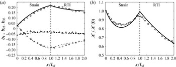
4.2. Comparison with the experiments of Gence and Mathieu
In the experiments of Gence & Mathieu (Reference Gence and Mathieu1979, Reference Gence and Mathieu1980), a plane strain is first applied to quasi-isotropic grid turbulence. A second strain is then applied, whose principal axes have been rotated by an angle
 ${\it\alpha}$
in the plane of the first strain. The mean-velocity gradients corresponding to the first and second strains are respectively
 $$\begin{eqnarray}{\it\lambda}=\left(\begin{array}{@{}ccc@{}}0 & 0 & 0\\ 0 & S & 0\\ 0 & 0 & -S\end{array}\right),\quad {\it\lambda}=\left(\begin{array}{@{}ccc@{}}0 & 0 & 0\\ 0 & S\cos (2{\it\alpha}) & -S\sin (2{\it\alpha})\\ 0 & -S\sin (2{\it\alpha}) & -S\cos (2{\it\alpha})\end{array}\right).\end{eqnarray}$$
In Gence & Mathieu (Reference Gence and Mathieu1980), the original experimental device is extended in such a way that the turbulence can develop downstream without a mean-velocity gradient. For these experiments,
 $S\simeq 2.9{\it\tau}_{0}^{-1}$
with
 ${\it\tau}_{0}=\mathscr{K}(0)/{\it\varepsilon}(0)$
, where the origin corresponds to the entrance of the distorting duct. The simulations are initialized with
 $Re_{{\it\lambda}}=60$
. No detailed spectral information is available in these works, and we assume that the turbulence is weakly axisymmetrically dilated at the entrance of the distorting duct. The initial condition is obtained from RDT and the degree of anisotropy is adjusted so that it coincides with the first measured values of the invariant
 $\mathit{II}$
defined by (4.5). Experimental data for the downstream evolution of the invariant
 $\mathit{II}$
are reported in figure 1 along with numerical results obtained with the system of governing equations (3.3)–(3.5). This figure shows a satisfactory agreement between experimental and numerical results, especially taking into account the uncertainty in the initial condition and a possible homogeneity fault in the experimental device. The first-order truncations in the description of anisotropy (§ 3.5) may also lie at the origin of discrepancies between experimental and numerical results. The system of governing equations (3.3)–(3.5) allows us to correctly capture the evolution of anisotropy, both in the straining regions and during the relaxation phases. Only the period of RTI for the angle
 ${\it\alpha}={\rm\pi}/4$
is not fully satisfactory, mainly because the boundary between the straining and relaxation regions in the experiments does not appear to be as clear as in the simulations. The case of straining without rotation in the second part of the distorting duct (
 ${\it\alpha}=0$
), followed by a relaxation phase, is further illustrated in figure 2. The present model properly captures the evolution of the anisotropy indicators
 $\unicode[STIX]{x1D623}_{ij}$
and that of the turbulent kinetic energy, both in the region dominated by linear effects and in the purely nonlinear one.
Evolution of the invariant
 $\mathit{II}$
versus the position in the distorting duct of length
 $L_{d}$
for the experiments of (a) Gence & Mathieu (Reference Gence and Mathieu1979) and (b) Gence & Mathieu (Reference Gence and Mathieu1980). Symbols correspond to experimental data and lines are obtained with the system of governing equations (3.3)–(3.5). Various values of the angle
 ${\it\alpha}$
between the principal axes of the two successive plane strains are investigated:
 ${\it\alpha}=0$
(▫, – - – - –),
 ${\it\alpha}={\rm\pi}/8$
(+,
 $\cdots \cdots$
),
 ${\it\alpha}={\rm\pi}/4$
(○,

 ${\it\alpha}=3{\rm\pi}/8$
(△, – – – –) and
 ${\it\alpha}={\rm\pi}/2$
(
 $\times$
, ——).
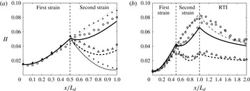
Evolution of (a) the anisotropy indicators
 $\unicode[STIX]{x1D623}_{11}$
(△, – – – –),
 $\unicode[STIX]{x1D623}_{22}$
(▫, – - – - –) and
 $\unicode[STIX]{x1D623}_{33}$
(○, ——) and (b) that of the turbulent kinetic energy
 $\mathscr{K}$
(○, ——) versus the position in the distorting duct of length
 $L_{d}$
for the experiment in Gence & Mathieu (Reference Gence and Mathieu1980) without rotation in the second part of the distorting duct (
 ${\it\alpha}=0$
). Symbols correspond to experimental data and lines are obtained with the system of governing equations (3.3)–(3.5).
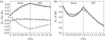
4.3. Turbulence subjected to a straining–relaxation–destraining cycle
The present model is further tested by comparing its predictions with the experiment of Chen et al. (Reference Chen, Meneveau and Katz2006), where a piston is used to apply plane straining and destraining on turbulence generated by active grids. The mean-velocity gradient in the experiment is of the form
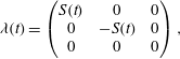 $$\begin{eqnarray}{\it\lambda}(t)=\left(\begin{array}{@{}ccc@{}}S(t) & 0 & 0\\ 0 & -S(t) & 0\\ 0 & 0 & 0\end{array}\right),\end{eqnarray}$$
where the temporal evolution of
 $S(t)$
is given by figure 3(a). Initially, the mean flow corresponds to plane straining (
 $S(t)>0$
), until
 $t/{\it\tau}_{0}\simeq 0.5$
. After a relaxation phase (
 $0.5\leqslant t/{\it\tau}_{0}\leqslant 0.7$
), destraining (
 $S(t)<0$
) is applied to the turbulence. In this experiment, the Taylor-microscale-based Reynolds number at the beginning of the straining cycle is
 $Re_{{\it\lambda}}\simeq 400$
. The maximum value of the strain
 $S(t)$
reached in the experiment is
 $\simeq 9.5{\it\tau}_{0}^{-1}$
. Figure 3(b) illustrates the temporal evolution of the anisotropy indicator
 $\tilde{\unicode[STIX]{x1D623}}_{11}(t)$
defined by (4.7). Experimental and numerical values obtained with the present model are reported, along with the RDT prediction, provided by Chen et al. (Reference Chen, Meneveau and Katz2006), corresponding to the mean flow defined by (4.12) and figure 3(a). The temporal evolution of
 $\tilde{\unicode[STIX]{x1D623}}_{11}(t)$
shows good agreement between the experiment and the present model. From the comparison with RDT results, it appears that nonlinear phenomena are significant on a quantitative level. This is partly due to the presence of a relaxation phase in the straining cycle. Thus, the validity of both linear and nonlinear contributions in the system of governing equations (3.3)–(3.5) can be confirmed by the comparison with this experiment.
(a) Temporal evolution of the strain
 $S(t)$
applied to the turbulence; (b) experimental values (○), numerical values obtained with the present model (——) and RDT prediction (– – – –) for the temporal evolution of the anisotropy indicator
 $\tilde{\unicode[STIX]{x1D623}}_{11}(t)$
in the experiment of Chen et al. (Reference Chen, Meneveau and Katz2006).
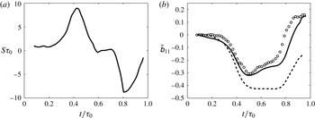
4.4. Turbulence subjected to axisymmetric expansion or contraction
We now consider the case of turbulence subjected to an axisymmetric expansion or contraction. The corresponding mean-velocity gradients are respectively
 $$\begin{eqnarray}{\it\lambda}=\left(\begin{array}{@{}ccc@{}}S/2 & 0 & 0\\ 0 & S/2 & 0\\ 0 & 0 & -S\end{array}\right),\quad {\it\lambda}=\left(\begin{array}{@{}ccc@{}}-S/2 & 0 & 0\\ 0 & -S/2 & 0\\ 0 & 0 & S\end{array}\right),\end{eqnarray}$$
with
 $S>0$
. These two configurations have been recently investigated in the DNS of Zusi & Perot (Reference Zusi and Perot2014), where both effects of axisymmetric expansion and contraction on initially approximately isotropic turbulence and its subsequent relaxation have been studied. We want to check whether the present model is able to reproduce one of the main observation of this paper: the two-stage RTI of turbulence after an axisymmetric expansion. In this configuration, it has been observed that the anisotropy continues to increase after the release of the strain during a short period of time, before decreasing in a more conventional way. The reader has to keep in mind that the microscale-based Reynolds number in this work is moderate (
 $Re_{{\it\lambda}}\simeq 50$
) and that two-stage RTI is observed only after an expansion with sufficiently high strain rate (
 $S\geqslant 3{\it\tau}_{0}^{-1}$
). A complete parametric study of this two-stage RTI should be performed, but this is beyond the scope of the present paper. Detailed numerical analyses of the RTI of axisymmetric turbulence can be found in Herring (Reference Herring1974), Chasnov (Reference Chasnov1995), Davidson, Okamoto & Kaneda (Reference Davidson, Okamoto and Kaneda2012) and Mons, Meldi & Sagaut (Reference Mons, Meldi and Sagaut2014).
Time evolution of the different components of the global anisotropy tensor
 $\unicode[STIX]{x1D623}_{ij}(t)$
(– – – –
 $\unicode[STIX]{x1D623}_{11}$
, – - – - –
 $\unicode[STIX]{x1D623}_{22}$
, ——
 $\unicode[STIX]{x1D623}_{33}$
) for (a) axisymmetric expansion and (b) contraction. The thick black lines correspond to numerical values obtained with the present model, while the thin black and grey lines refer to the DNS results of Zusi & Perot (Reference Zusi and Perot2014) for two different initial conditions. The vertical dotted line marks the time at which strain is released.
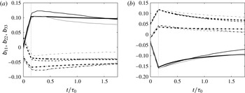
First, a quantitative comparison between the predictions of the present model and the DNS results of Zusi & Perot (Reference Zusi and Perot2014) is performed. Zusi & Perot (Reference Zusi and Perot2014) use two different initial conditions in their work which are difficult to characterize. Besides, these initial fields are anisotropic and non-axisymmetric. Predictions concerning the time evolution of the different components of the tensor
 $\unicode[STIX]{x1D623}_{ij}(t)$
obtained with the present model and the DNS of Zusi & Perot (Reference Zusi and Perot2014) are reported in figure 4. Both expansion and contraction cases are investigated with
 $S\simeq 3.4{\it\tau}_{0}^{-1}$
, and simulations are initialized with
 $Re_{{\it\lambda}}=50$
. The production periods are well recovered by the model. In the RTI regions, significant discrepancies between the DNS results obtained with the two initial fields can be noticed, and the results obtained with the present model lie between these two predictions. Thus, given the uncertainties in the initial condition and a potential additional source of discrepancies originating from the limitation to moderate anisotropy of the present model (§ 3.5), these comparisons are relatively satisfactory. In particular, the major difference between the expansion and contraction cases is recovered: after the release of the strain, the anisotropy immediately decreases in the contraction case, whereas it slightly increases in the expansion case before decreasing. To further illustrate this observation, complementary runs are performed starting from initially isotropic turbulence, instead of an anisotropic and non-axisymmetric field, in order to get clearer results.
(a,c) Time evolution of the anisotropy indicator
 $\unicode[STIX]{x1D623}_{33}(t)$
(

 $\unicode[STIX]{x1D623}_{33}^{(dir)}(k,t)$
(——) and
 $\unicode[STIX]{x1D623}_{33}^{(pol)}(k,t)$
(– – – –) with that of their time derivatives; (a,b) and (c,d) correspond to the axisymmetric expansion and contraction cases respectively. The vertical dotted line marks the time at which strain is released.
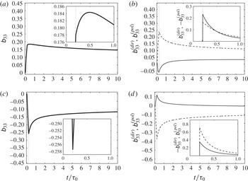
Figures 5 and 6 illustrate numerical results obtained with the present model for initially isotropic turbulence submitted to an axisymmetric expansion or contraction and then released. Simulations are initialized with
 $Re_{{\it\lambda}}=50$
and we set
 $S=5{\it\tau}_{0}^{-1}$
. The axisymmetric expansion or contraction is maintained from
 $t=0$
to
 $St=1$
. We first consider the results for axisymmetric expansion, which are reported in figures 5(a,b) and 6(a). The temporal evolution of the anisotropy indicator
 $\unicode[STIX]{x1D623}_{33}(t)$
is given in figure 5(a). Since we consider axisymmetric turbulence, the tensor
 $\unicode[STIX]{x1D623}_{ij}(t)$
is diagonal, with
 $\unicode[STIX]{x1D623}_{33}(t)=-\unicode[STIX]{x1D623}_{11}(t)/2=-\unicode[STIX]{x1D623}_{22}(t)/2$
. As observed above,
 $\unicode[STIX]{x1D623}_{33}(t)$
slightly increases after the release of the strain before decaying. Further insight into this two-stage RTI is given by figure 5(b), where the temporal evolution of the directivity and polarization components of
 $\unicode[STIX]{x1D623}_{33}(t)=\unicode[STIX]{x1D623}_{33}^{(dir)}(t)+\unicode[STIX]{x1D623}_{33}^{(pol)}(t)$
is reported, along with their time derivatives. Contrary to
 $\unicode[STIX]{x1D623}_{33}(t)$
, both
 $\unicode[STIX]{x1D623}_{33}^{(dir)}(t)$
and
 $\unicode[STIX]{x1D623}_{33}^{(pol)}(t)$
immediately decay in magnitude after the release of the strain. However, since
 $\unicode[STIX]{x1D623}_{33}^{(dir)}(t)$
is negative, whereas both
 $\unicode[STIX]{x1D623}_{33}^{(pol)}(t)$
and
 $\unicode[STIX]{x1D623}_{33}(t)$
are positive, and it first decreases in magnitude at a faster rate than
 $\unicode[STIX]{x1D623}_{33}^{(pol)}(t)$
, the total anisotropy indicator
 $\unicode[STIX]{x1D623}_{33}(t)$
increases. As soon as the polarization component decays at a faster rate than the directivity one, the global anisotropy decreases. The difference in the relaxation rates between directional anisotropy and polarization anisotropy in the present model, which lies at the origin of the increase of the total anisotropy, may be related to the difference in the relaxation rates between the dimensionality and circulicity tensors in Kassinos & Reynolds (Reference Kassinos and Reynolds1997) and Kassinos et al. (Reference Kassinos, Reynolds and Rogers2001) (see appendix A for further details).
The case of RTI after an axisymmetric contraction is illustrated in figures 5(c,d) and 6(b). The anisotropy indicator
 $\unicode[STIX]{x1D623}_{33}(t)$
decays in magnitude immediately after the release of the strain, as
 $\unicode[STIX]{x1D623}_{33}^{(dir)}(t)$
and
 $\unicode[STIX]{x1D623}_{33}^{(pol)}(t)$
do. The polarization component, of the same sign as
 $\unicode[STIX]{x1D623}_{33}(t)$
, decays in magnitude at a faster rate than the directivity one as soon as the strain is released. The qualitative difference in the RTI between expansion and contraction is even more striking by looking at figure 6(a,b), where the evolution of the invariant
 $\mathit{II}(t)$
is indicated for the expansion and contraction cases respectively. The temporal evolution of the invariant
 $\mathit{III}(t)$
and that of the ratio
 ${\it\rho}(t)$
between the characteristic times of decay and RTI defined by (4.6) are reported in figure 6(c,d). The expansion case is associated with a positive value for
 $\mathit{III}(t)$
(axial component
 $\langle u_{3}u_{3}\rangle (t)$
greater than the transverse ones), whereas
 $\mathit{III}(t)$
is negative in the contraction case. Figure 6(d) indicates that the RTI process is slower in the expansion case than in the contraction case (
 ${\it\rho}(t)$
takes a greater value if the RTI is faster and is negative during the slight increase of anisotropy in the expansion case). This result is consistent with the discussions in Gence (Reference Gence1983) and Choi & Lumley (Reference Choi and Lumley2001).
(a,b) Temporal evolution of the invariant
 $\mathit{II}(t)$
(——) for the axisymmetric (a) expansion and (b) contraction cases; (c,d) temporal evolution of (c) the invariant
 $\mathit{III}(t)$
and (d) the ratio
 ${\it\rho}(t)$
between characteristic times of decay and RTI for the expansion (– - – - –) and contraction (——) cases. The vertical dotted line marks the time at which strain is released.
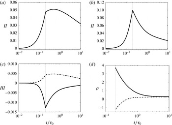
4.5. The RTI of shear-released turbulence
The RTI of initially isotropic (Saffman) turbulence that is suddenly subjected to a mean shear and is then released is investigated. The mean-velocity gradient that corresponds to the application of a shear on the turbulent flow is
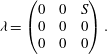 $$\begin{eqnarray}{\it\lambda}=\left(\begin{array}{@{}ccc@{}}0 & 0 & S\\ 0 & 0 & 0\\ 0 & 0 & 0\end{array}\right).\end{eqnarray}$$
The simulations are initialized with
 $Re_{{\it\lambda}}=10^{4}$
. The anisotropy of the flow is introduced by using either the RDT solution for homogeneous shear flow with
 $St=0.42$
(this value allows us to observe a significant departure from isotropy of the diagonal components of the Reynolds stress tensor) or the linear terms of (3.3)–(3.5) with
 $S=10{\it\tau}_{0}^{-1}$
if
 $t<0.042{\it\tau}_{0}$
and
 $S=0$
if not, starting from an isotropic field. Results are illustrated in figures 7–9.
Global anisotropy indicators ——
 $\unicode[STIX]{x1D623}_{ij}$
,

 $\unicode[STIX]{x1D623}_{ij}^{(dir)}$
and – - – - –
 $\unicode[STIX]{x1D623}_{ij}^{(pol)}$
in the case of shear-released Saffman turbulence. The grey lines correspond to the use of RDT solutions for the initialization, whereas the black lines correspond to the use of the linear terms in (3.3)–(3.5) for the introduction of anisotropy. The vertical black dotted line marks the limit at
 $t=0.042{\it\tau}_{0}$
after which the shear is released when the linear terms are used.
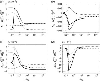
(a) Energy spectrum
 $E(k,t)$
, (b) cross-correlation spectrum
 ${\it\varphi}_{13}(k,t)$
and spectra (c)
 $\unicode[STIX]{x1D60F}_{13}^{(dir)}(k,t)$
, (d)
 $\unicode[STIX]{x1D60F}_{13}^{(pol)}(k,t)$
, (e)
 $\unicode[STIX]{x1D60F}_{33}^{(dir)}(k,t)$
and (f)
 $\unicode[STIX]{x1D60F}_{33}^{(pol)}(k,t)$
for shear-released Saffman turbulence. The RDT is used for the initialization. The curves have been sampled at the normalized time:

 $t/{\it\tau}_{0}=0$
;

 $t/{\it\tau}_{0}=10^{-3}$
; – - – - –
 $t/{\it\tau}_{0}=10^{-2}$
;
 $\cdots \cdots$
 $t/{\it\tau}_{0}=10^{-1}$
; – – – –
 $t/{\it\tau}_{0}=1$
; ——
 $t/{\it\tau}_{0}=10$
.
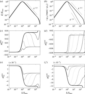
Budget terms of the equation
 $(\partial /\partial t){\it\varphi}_{ij}(k,t)=-2{\it\nu}k^{2}{\it\varphi}_{ij}(k,t)+\unicode[STIX]{x1D617}_{ij}(k,t)+\unicode[STIX]{x1D61A}_{ij}(k,t)$
, premultiplied by
 $k$
(– - – - –
 $k\unicode[STIX]{x1D61A}_{ij}(k,t)$
;
 $\cdots \cdots$
 $-2{\it\nu}k^{3}{\it\varphi}_{ij}(k,t)$
; – – – –
 $k\unicode[STIX]{x1D617}_{ij}(k,t)$
; ——
 $k(\partial /\partial t){\it\varphi}_{ij}(k,t)$
), and normalized by
 $\max _{k}(|k(\partial /\partial t){\it\varphi}_{ij}(k,t)|)$
. Shear-released Saffman turbulence is considered and the RDT is used for the initialization; (a,c) refer to the component
 ${\it\varphi}_{13}(k,t)$
, whereas (b,d) refer to the component
 ${\it\varphi}_{33}(k,t)$
. The budget terms have been sampled at the normalized time
 $t/{\it\tau}_{0}=10^{-1}$
(a,b) and
 $t/{\it\tau}_{0}=10$
(c,d).
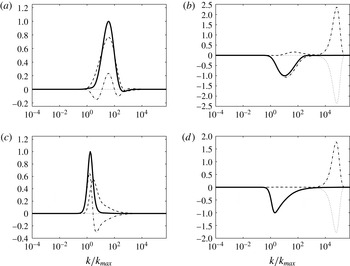
It appears from figure 7 that solutions initialized with RDT or with the linear terms (3.7)–(3.9) coincide, which confirms the validity of the linear terms of the present model in the case of homogeneous shear turbulence. The evolution of anisotropy is similar to that in the case of axisymmetric Saffman turbulence (Chasnov Reference Chasnov1995; Davidson et al.
Reference Davidson, Okamoto and Kaneda2012; Mons et al.
Reference Mons, Meldi and Sagaut2014). After a transient regime which corresponds to the RTI of small scales, an asymptotic anisotropic state is reached due to the fulfilment of the PLE hypothesis (
 $E(k,t)=E(k,0)$
for
 $k\ll k_{max}(t)$
if
 $1\leqslant {\it\sigma}\leqslant 3$
with
 $E(k\rightarrow 0,t)\propto k^{{\it\sigma}}$
). A similar behaviour was also observed with the model of Clark & Zemach (Reference Clark and Zemach1995) for the relaxation of turbulence after the release of plane strain. Even the off-diagonal component
 $\unicode[STIX]{x1D623}_{13}(t)$
converges towards a non-zero value, which means that the cross-correlation
 $\langle u_{1}u_{3}\rangle (t)$
is maintained even though the mean shear is released.
The RTI of small scales during the transient regime is illustrated in figure 8 for the components of the spherically integrated second-order spectral tensor defined by (1.4),
 ${\it\varphi}_{13}(k,t)$
and
 ${\it\varphi}_{33}(k,t)$
. Both the directional anisotropy and the polarization anisotropy become negligible in the inertial range for
 $t\geqslant 10{\it\tau}_{0}$
. This result is also valid for the diagonal components
 ${\it\varphi}_{11}(k,t)$
and
 ${\it\varphi}_{22}(k,t)$
that are not illustrated here. Figure 8(b) indicates that the initial cross-correlation spectrum
 ${\it\varphi}_{13}(k,0)$
given by RDT evolves like
 $k^{-5/3}$
in the inertial range. Then, due to purely nonlinear processes, this shape is modified and evolves like
 $k^{-7/3}$
at
 $t=10{\it\tau}_{0}$
. This result is consistent with the predictions of Lumley (Reference Lumley1967), Leslie (Reference Leslie1973), Yoshida et al. (Reference Yoshida, Ishihara and Kaneda2003) and Weinstock (Reference Weinstock2013).
The budget terms of the governing equation (4.8) are reported in figure 9 for the spectra
 ${\it\varphi}_{13}(k,t)$
and
 ${\it\varphi}_{33}(k,t)$
at
 $t=0.1{\it\tau}_{0}$
and
 $t=10{\it\tau}_{0}$
. During the transient regime corresponding to the RTI of small scales (
 $t=0.1{\it\tau}_{0}$
), the nonlinear pressure–strain rate tensor
 $\unicode[STIX]{x1D617}_{ij}(k,t)$
has a significant influence in the inertial range. Its contribution is positive for the negative cross-correlation spectrum
 ${\it\varphi}_{13}(k,t)$
, which would be identically zero in the isotropic case, and also positive for the spectrum
 ${\it\varphi}_{33}(k,t)$
, since this component has been relatively damped by the mean shear via linear effects. Once small scales have returned to isotropy (
 $t=10{\it\tau}_{0}$
), the contribution of
 $\unicode[STIX]{x1D617}_{ij}(k,t)$
is negligible
 $\forall k$
for the component
 ${\it\varphi}_{33}(k,t)$
(as well as for the other diagonal components), even though large scales have not returned to isotropy. The shape of the transfer term
 $\unicode[STIX]{x1D61A}_{33}(k,t)$
is then virtually identical to that in the isotropic case. Concerning the cross-correlation component, nonlinear terms act predominantly at scales close to the integral length scale. These results are consistent with previous studies dealing with the RTI of Saffman turbulence, where it is observed that small scales quickly return to isotropy after the release of the shear/strain, whereas large scales fully retain anisotropy due to the fulfilment of the PLE hypothesis.
Temporal evolutions of (a) the different components of the global anisotropy tensor
 $\unicode[STIX]{x1D623}_{ij}(t)$
and the ratio
 ${\it\varepsilon}/S\mathscr{K}$
(– – – –
 $\unicode[STIX]{x1D623}_{11}$
, ——
 $\unicode[STIX]{x1D623}_{13}$
,
 $\cdots \cdots$
 $\unicode[STIX]{x1D623}_{22}$
, – - – - –
 $\unicode[STIX]{x1D623}_{33}$
and

 ${\it\varepsilon}/S\mathscr{K}$
) and (b) those of the turbulent kinetic energy
 $\mathscr{K}(t)$
(——),
 $k_{max}$
(– – – –) and
 $E_{max}$
(– - – - –) defined in (4.10) and normalized by their initial values for homogeneous shear turbulence. The grey curves are plotted with
 ${\it\gamma}=0.337$
.
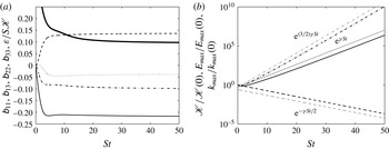
(a) Energy spectrum
 $E(k,t)$
and (b) cross-correlation spectrum
 ${\it\varphi}_{13}(k,t)$
at
 $St=0$
(thick black line) and
 $St=15$
(thin black lines). (c–f) Budget terms of the governing equation
 $(\partial /\partial t){\it\varphi}_{ij}(k,t)=-2{\it\nu}k^{2}{\it\varphi}_{ij}(k,t)+\unicode[STIX]{x1D617}_{ij}(k,t)+\unicode[STIX]{x1D61A}_{ij}(k,t)+\unicode[STIX]{x1D613}_{ij}(k,t)$
, premultiplied by
 $k$
(– - – - –
 $k\unicode[STIX]{x1D61A}_{ij}(k,t)$
;
 $\cdots \cdots$
 $-2{\it\nu}k^{3}{\it\varphi}_{ij}(k,t)$
; – – – –
 $k\unicode[STIX]{x1D617}_{ij}(k,t)$
; ——
 $k\unicode[STIX]{x1D613}_{ij}(k,t)$
;

 $k(\partial /\partial t){\it\varphi}_{ij}(k,t)$
), and normalized by
 $\max _{k}(|k(\partial /\partial t){\it\varphi}_{ij}(k,t)|)$
. The curves are sampled at
 $St=50$
for homogeneous shear turbulence and refer to the components (c)
 ${\it\varphi}_{11}(k,t)$
, (d)
 ${\it\varphi}_{13}(k,t)$
, (e)
 ${\it\varphi}_{22}(k,t)$
and (f)
 ${\it\varphi}_{33}(k,t)$
. The position of the shear scale
 $L_{s}$
is also shown by vertical grey dashed lines.
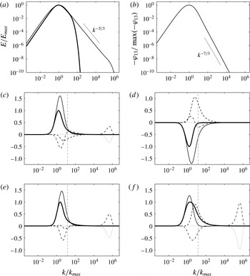
Energy spectrum (a–c) and maximal eigenvalue of the tensor
 $\unicode[STIX]{x1D60F}_{ij}^{(dir)}(k,t)$
(d–f) for the different test cases investigated in this paper. The value
 $1/15$
from the criterion (3.17) is displayed as dashed lines. (a,d) The case of plane straining (case
 ${\it\alpha}={\rm\pi}/8$
of figure 1
a); the curves are sampled at the end of the simulation (
 $St\simeq 1.4$
). (b,e) The case of axisymmetric expansion of figure 4(a) (
 $St=0.5$
). (c,f) Results concerning homogeneous shear turbulence (figures 10 and 11); the curves are sampled at
 $St=50$
.

4.6. Homogeneous shear turbulence
Finally, we address the case of homogeneous turbulence subjected to a constant maintained mean shear. The corresponding mean-velocity gradient is given by (4.14). Weinstock (Reference Weinstock2013) performed an exhaustive analytical study of this configuration in 3D Fourier space, without limitations on time or wavenumber. In this subsection, it is checked that the present model is able to recover results established in this prior work, among others. The corresponding simulation realized with the present model is initialized with
 $Re_{{\it\lambda}}=50$
, the shear rate is fixed at
 $S=2{\it\tau}_{0}^{-1}$
and the turbulence is initially isotropic. The temporal evolutions of the components of the deviatoric tensor
 $\unicode[STIX]{x1D623}_{ij}(t)$
and that of the kinetic energy
 $\mathscr{K}(t)$
are reported in figure 10. The different components
 $\unicode[STIX]{x1D623}_{ij}(t)$
and the ratio
 ${\it\varepsilon}(t)/S\mathscr{K}(t)$
reach constant values after
 $St\approx 20$
, as observed in, e.g., Weinstock (Reference Weinstock2013). Considering the governing equation for the turbulent kinetic energy
 $\mathscr{K}(t)$
,
 $$\begin{eqnarray}\frac{\text{d}}{\text{d}t}\mathscr{K}(t)=-2S\mathscr{K}(t)\unicode[STIX]{x1D623}_{13}(t)-{\it\varepsilon}(t),\end{eqnarray}$$
one can deduce that for
 $St\geqslant 20$
 $$\begin{eqnarray}\mathscr{K}(t)\sim \text{e}^{{\it\gamma}St},\quad {\it\gamma}=\text{const.}=-2\unicode[STIX]{x1D623}_{13}-\frac{{\it\varepsilon}}{\mathscr{K}S}.\end{eqnarray}$$
As illustrated in figure 10(b), the results obtained with the present model are consistent with such an exponential growth of the kinetic energy. The model also predicts the temporal evolutions of the peak of the energy spectrum
 $E_{max}$
and the corresponding wavenumber
 $k_{max}$
defined in (4.10) as
 $E_{max}(t)\sim \text{e}^{(3/2){\it\gamma}St}$
and
 $k_{max}(t)\sim \text{e}^{-{\it\gamma}St/2}$
. All of these results are consistent with dimensional analysis and with the study performed in Weinstock (Reference Weinstock2013), in which
 ${\it\gamma}=0.115$
. The estimated value of the growth rate
 ${\it\gamma}$
in a set of experiments (Tavoularis & Corrsin Reference Tavoularis and Corrsin1981; Tavoularis & Karnik Reference Tavoularis and Karnik1989) ranges between 0.08 and 0.12, whereas values between 0.1 and 0.2 can be found in DNS studies (Rogers et al.
Reference Rogers, Moin and Reynolds1986; Brethouwer Reference Brethouwer2005; Isaza & Collins Reference Isaza and Collins2009). Although a clear consensus about the value of the growth rate
 ${\it\gamma}$
cannot be found in the literature, and its sensitivity with respect to initial conditions, Reynolds number and shear rate has to be further investigated, the present model overestimates
 ${\it\gamma}$
(
 $\simeq 0.337$
) in comparison with values found in the literature. This lack of quantitative agreement originates from the first-order truncations in the description of anisotropy (§ 3.5). Compared with previous test cases considered in the present paper, the cumulated shear reached in the simulation illustrated in figures 10 and 11 is much higher (see § 4.7), which provides asymptotic information at high Reynolds numbers. Concerning results in spectral space, the kinetic energy spectrum
 $E(k,t)$
at
 $St=50$
(figure 11
a) displays a
 $-5/3$
slope in the inertial range, as reported in experiments or DNS. Figure 11(b) reports the cross-correlation spectrum
 ${\it\varphi}_{13}(k,t)$
at
 $St=50$
. The latter evolves like
 $k^{-7/3}$
in the inertial range, as predicted theoretically (Lumley Reference Lumley1967; Leslie Reference Leslie1973; Yoshida et al.
Reference Yoshida, Ishihara and Kaneda2003; Weinstock Reference Weinstock2013) and observed in the experiments of Shen & Warhaft (Reference Shen and Warhaft2000) and the DNS of Ishihara et al. (Reference Ishihara, Yoshida and Kaneda2002). This result supports a posteriori the choice of eddy damping (2.26) and (2.27). The budget terms of the governing equation (4.8) are illustrated in figure 11(c–f). The position of the shear scale
 $L_{s}=\sqrt{{\it\varepsilon}/S^{3}}$
(Corrsin Reference Corrsin1958) is also reported in the figures. For
 $1/L\leqslant k\leqslant 1/L_{s}$
, the flow is expected to be dominated by production terms, whereas for
 $k\geqslant 1/L_{s}$
, the contribution of nonlinear transfers should prevail. This interpretation is reasonably well supported by the present results. Figure 11(c–f) can help in visualizing the nonlinear process that lies at the origin of the exponential growth of the turbulent kinetic energy. Since the component
 ${\it\varphi}_{33}(k,t)$
is less fed than the other diagonal components by the mean shear, the nonlinear pressure–strain rate tensor
 $\unicode[STIX]{x1D617}_{33}(k,t)$
is strongly positive and redistributes energy from the components
 ${\it\varphi}_{11}(k,t)$
and
 ${\it\varphi}_{22}(k,t)$
to
 ${\it\varphi}_{33}(k,t)$
(
 $\unicode[STIX]{x1D617}_{ii}(k,t)=0\;\forall k,t$
). Since the cross-correlation component of the Reynolds stress tensor
 $2\unicode[STIX]{x1D612}_{13}(t)$
is fed by the mean shear via the term
 $-2S\unicode[STIX]{x1D612}_{33}(t)$
, its production is enhanced, allowing an increase of the growth rate of the turbulent kinetic energy
 $\mathscr{K}(t)$
via the term
 $-2S\mathscr{K}(t)\unicode[STIX]{x1D623}_{13}(t)=-2S\unicode[STIX]{x1D612}_{13}(t)$
.
4.7. Realizability condition
Due to spherical integration and truncation of expansions (3.14) and (3.15), the present model is limited to moderate anisotropy, and the criterion (3.17) is derived in § 3.5 in order to quantify the upper boundary of anisotropy intensity that can be investigated with the representation (3.2) and the corresponding system of governing equations (3.3)–(3.5). In this last subsection, it is checked that the different test cases considered in this paper can be described using the representation (3.2) and (3.3)–(3.5). Figure 12 reports the criterion (3.17) for typical flow configurations investigated in this paper: plane straining, axisymmetric expansion and pure plane shear. Rather than the absolute value of the typical strain or shear rate
 $S$
, it is the accumulated strain/shear
 $St$
that gives a good estimation of the anisotropy introduced in the flow. The interplay between linear and nonlinear contributions in (3.3)–(3.5) also affects the evolution of anisotropy in the flow, but this effect must be studied on a case-by-case basis in view of the significant differences that exist between, e.g., rotational and irrotational mean flows (Sagaut & Cambon Reference Sagaut and Cambon2008). It is worth keeping in mind that for the purpose of spherical integration, the same representation (3.2) is used for both linear contributions and transfer terms in (2.12) and (2.13), the latter being closed by the EDQNM. The different cases of plane straining/destraining investigated in this paper are associated with small values for the accumulated strain. Figure 12(d) illustrates the case
 ${\it\alpha}={\rm\pi}/8$
of figure 1(a) from the experiments of Gence and Mathieu. This configuration corresponds to the accumulated strain
 $St\simeq 1.4$
, and the anisotropy of the flow at all scales is significantly lower than the upper bound of (3.17). This result is similar for the other cases of plane straining/destraining in this paper. The case of axisymmetric expansion of figure 4(a) is investigated in figure 12(e). The accumulated strain is
 $St=0.5$
and the criterion (3.17) is respected at all scales. The same applies to the axisymmetric contraction case. Finally, the case of homogeneous shear turbulence is illustrated in figure 12(f) at
 $St=50$
, and criterion (3.17) is verified at all scales. Thus, all of the flow configurations considered in the present paper can be described by the representation (3.2) and the corresponding system of governing equations (3.3)–(3.5).
5. Conclusion and perspectives
Modelling of anisotropy in homogeneous flows has been considered at two different levels. The first one is the three-dimensional spectral level, in which a decomposition of the spectral tensor for arbitrary anisotropy lends support to a splitting of anisotropy at any subsequent level in terms of directional anisotropy and polarization anisotropy. In a second step, a model for spherically integrated quantities has been proposed, which is based on 11 coupled equations. It is dedicated to turbulent flows where the anisotropy is moderate and where linear effects induced by mean-velocity gradients play a negligible role in the dynamics of triple correlations compared with the induced production effects in the equations for the second-order correlations. This model is not restricted to a particular symmetry and can be used for a wide range of flow configurations, as illustrated by the different applications of the model considered in this paper. A satisfactory agreement with the experiments of Gence & Mathieu (Reference Gence and Mathieu1979, Reference Gence and Mathieu1980) has been observed, which confirms the capability of the model to account for production of anisotropy by mean-flow gradients.
Concerning the RTI of initially deformed or sheared turbulence, the model is consistent with the PLE and ensures correct rapid RTI of the smallest scales. Different relaxation rates for directional anisotropy and polarization anisotropy allow us to correctly interpret the apparent delay in the RTI after axisymmetric expansion (Zusi & Perot Reference Zusi and Perot2014). In addition, our model fits well the recent experiment of Chen et al. (Reference Chen, Meneveau and Katz2006) with a non-stationary straining cycle. For turbulence continuously subjected to a pure plane shear, the model ensures a correct asymptotic regime with constant values for the components of the dimensionless deviatoric tensor
 $\unicode[STIX]{x1D623}_{ij}(t)$
associated with the Reynolds stress tensor. In addition, it can reproduce the exponential growth of the turbulent kinetic energy mediated by nonlinear pressure redistribution terms. However, first-order truncations in the description of anisotropy, which are the main sources of possible discrepancies between the present model and DNS/experimental results, prevent a good quantitative agreement with typical values of the growth rate found in the literature. For this configuration, an alternative approach, which is entirely formulated in 3D Fourier space and without limitation in time, can be found in Weinstock (Reference Weinstock2013).
Beyond moderate anisotropy, a more complex version of the model could possibly combine exact linear operators in
 $\boldsymbol{k}$
-vectors, as in the left-hand side of (2.12)–(2.13), with transfer terms only generated by low-order angular harmonic expansions. Such a model could reproduce the dominant RDT dynamics for the largest scales, and the quasi-isotropic behaviour for scales smaller than a Corrsin scale.
Appendix A. Relationships between two-point spectral tensors and single-point tensors
The equations addressed in this paper involve several tensors: production by mean-velocity gradients, dissipation, transfer, pressure–strain rate. In the following, we give their expressions systematically in terms of
 $\boldsymbol{k}$
, then in terms of
 $k$
, obtained by spherically averaging the first one, and their final single-point contribution obtained by integrating on
 $k$
, as in full Reynolds stress models (RSMs) with an additional structure-based tensor. Time dependence is implied (not explicitly written below).
A.1. Production term by space-uniform mean-velocity gradient
The production term by the space-uniform mean-velocity gradient in (2.3) is
 ${\it\lambda}_{il}\hat{\unicode[STIX]{x1D619}}_{lj}(\boldsymbol{k})+{\it\lambda}_{jl}\hat{\unicode[STIX]{x1D619}}_{li}(\boldsymbol{k})$
. By using the representation (3.1), its spherically integrated counterpart is
 $$\begin{eqnarray}\iint _{S_{k}}{\it\lambda}_{il}\hat{\unicode[STIX]{x1D619}}_{lj}(\boldsymbol{k})+{\it\lambda}_{jl}\hat{\unicode[STIX]{x1D619}}_{il}(\boldsymbol{k})\,\text{d}^{2}\boldsymbol{k}=\frac{4}{3}\unicode[STIX]{x1D61A}_{ij}E+2E\left(\!{\it\lambda}_{il}\unicode[STIX]{x1D60F}_{lj}^{(dir)}+{\it\lambda}_{jl}\unicode[STIX]{x1D60F}_{li}^{(dir)}\!\right)+2E\left(\!{\it\lambda}_{il}\unicode[STIX]{x1D60F}_{lj}^{(pol)}+{\it\lambda}_{jl}\unicode[STIX]{x1D60F}_{li}^{(pol)}\!\right),\end{eqnarray}$$
with
 $E=E(k)$
,
 $\unicode[STIX]{x1D60F}_{ij}^{(dir)}=\unicode[STIX]{x1D60F}_{ij}^{(dir)}(k)$
and
 $\unicode[STIX]{x1D60F}_{ij}^{(pol)}=\unicode[STIX]{x1D60F}_{ij}^{(pol)}(k)$
. The single-point counterpart of the production term is given by
 $$\begin{eqnarray}\displaystyle \iiint {\it\lambda}_{il}\hat{\unicode[STIX]{x1D619}}_{lj}(\boldsymbol{k})+{\it\lambda}_{jl}\hat{\unicode[STIX]{x1D619}}_{il}(\boldsymbol{k})\,\text{d}^{3}\boldsymbol{k} & = & \displaystyle \frac{4}{3}\unicode[STIX]{x1D61A}_{ij}\mathscr{K}+2\mathscr{K}\left({\it\lambda}_{il}\unicode[STIX]{x1D623}_{lj}^{(dir)}+{\it\lambda}_{jl}\unicode[STIX]{x1D623}_{li}^{(dir)}\right)\nonumber\\ \displaystyle & & \displaystyle +\,2\mathscr{K}\left({\it\lambda}_{il}\unicode[STIX]{x1D623}_{lj}^{(pol)}+{\it\lambda}_{jl}\unicode[STIX]{x1D623}_{li}^{(pol)}\right),\end{eqnarray}$$
where the tensors
 $\unicode[STIX]{x1D623}_{ij}^{(dir)}$
and
 $\unicode[STIX]{x1D623}_{ij}^{(pol)}$
are defined by (4.4).
A.2. Dissipation term
The dissipation term in (2.3) is
 $2{\it\nu}k^{2}\hat{\unicode[STIX]{x1D619}}_{ij}(\boldsymbol{k})$
. Its spherically integrated counterpart is
 $$\begin{eqnarray}\iint _{S_{k}}2{\it\nu}k^{2}\hat{\unicode[STIX]{x1D619}}_{ij}(\boldsymbol{k})\,\text{d}^{2}\boldsymbol{k}=4{\it\nu}k^{2}E\left(\frac{{\it\delta}_{ij}}{3}+\unicode[STIX]{x1D60F}_{ij}^{(dir)}+\unicode[STIX]{x1D60F}_{ij}^{(pol)}\right).\end{eqnarray}$$
The corresponding single-point contribution is
 $$\begin{eqnarray}\iiint 2{\it\nu}k^{2}\hat{\unicode[STIX]{x1D619}}_{ij}(\boldsymbol{k})\,\text{d}^{3}\boldsymbol{k}=\frac{2}{3}{\it\delta}_{ij}{\it\varepsilon}+{\it\varepsilon}_{ij}^{(dir)}+{\it\varepsilon}_{ij}^{(pol)},\end{eqnarray}$$
where
 ${\it\varepsilon}_{ij}^{(dir)}=\int _{0}^{\infty }4{\it\nu}k^{2}E(k)\unicode[STIX]{x1D60F}_{ij}^{(dir)}(k)\,\text{d}k$
, with a similar definition for
 ${\it\varepsilon}_{ij}^{(pol)}$
.
A.3. ‘Rapid’ contribution of the pressure–strain rate tensor
The rapid contribution of the pressure–strain rate tensor is given by
 $2{\it\lambda}_{ln}{\it\alpha}_{l}({\it\alpha}_{i}\hat{\unicode[STIX]{x1D619}}_{nj}(\boldsymbol{k})+{\it\alpha}_{j}\hat{\unicode[STIX]{x1D619}}_{ni}(\boldsymbol{k}))$
. Its spherically integrated counterpart is
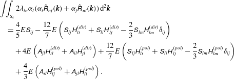 $$\begin{eqnarray}\displaystyle & & \displaystyle \iint _{S_{k}}2{\it\lambda}_{ln}{\it\alpha}_{l}({\it\alpha}_{i}\hat{\unicode[STIX]{x1D619}}_{nj}(\boldsymbol{k})+{\it\alpha}_{j}\hat{\unicode[STIX]{x1D619}}_{ni}(\boldsymbol{k}))\,\text{d}^{2}\boldsymbol{k}\nonumber\\ \displaystyle & & \displaystyle \quad =\frac{4}{5}E\unicode[STIX]{x1D61A}_{ij}-\frac{12}{7}E\left(\unicode[STIX]{x1D61A}_{lj}\unicode[STIX]{x1D60F}_{li}^{(dir)}+\unicode[STIX]{x1D61A}_{li}\unicode[STIX]{x1D60F}_{lj}^{(dir)}-\frac{2}{3}\unicode[STIX]{x1D61A}_{lm}\unicode[STIX]{x1D60F}_{lm}^{(dir)}{\it\delta}_{ij}\right)\nonumber\\ \displaystyle & & \displaystyle \qquad +\,4E\left(\unicode[STIX]{x1D608}_{jl}\unicode[STIX]{x1D60F}_{il}^{(dir)}+\unicode[STIX]{x1D608}_{il}\unicode[STIX]{x1D60F}_{jl}^{(dir)}\right)+\frac{12}{7}E\left(\unicode[STIX]{x1D61A}_{lj}\unicode[STIX]{x1D60F}_{li}^{(pol)}+\unicode[STIX]{x1D61A}_{li}\unicode[STIX]{x1D60F}_{lj}^{(pol)}-\frac{2}{3}\unicode[STIX]{x1D61A}_{lm}\unicode[STIX]{x1D60F}_{lm}^{(pol)}{\it\delta}_{ij}\right)\nonumber\\ \displaystyle & & \displaystyle \qquad +\,\frac{4}{3}E\left(\unicode[STIX]{x1D608}_{il}\unicode[STIX]{x1D60F}_{lj}^{(pol)}+\unicode[STIX]{x1D608}_{jl}\unicode[STIX]{x1D60F}_{li}^{(pol)}\right).\end{eqnarray}$$
Similarly to the transition from (A 1) to (A 2), the single-point contribution of the rapid component of the pressure–strain rate tensor is obtained from (A 5) by replacing
 $E(k)$
,
 $\unicode[STIX]{x1D60F}_{ij}^{(dir)}(k)$
and
 $\unicode[STIX]{x1D60F}_{ij}^{(pol)}(k)$
with
 $\mathscr{K}$
,
 $\unicode[STIX]{x1D623}_{ij}^{(dir)}$
and
 $\unicode[STIX]{x1D623}_{ij}^{(pol)}$
respectively. The closure of the rapid pressure–strain rate tensor in RSMs is generally applied to the tensor
 $\unicode[STIX]{x1D614}_{ijpq}$
, defined by
 $$\begin{eqnarray}\unicode[STIX]{x1D614}_{ijpq}=\iiint {\it\alpha}_{p}{\it\alpha}_{q}\hat{\unicode[STIX]{x1D619}}_{ij}(\boldsymbol{k})\,\text{d}^{3}\boldsymbol{k},\end{eqnarray}$$
and made non-dimensional by the turbulent kinetic energy. The closure is usually in terms of the deviatoric tensor
 $\unicode[STIX]{x1D623}_{ij}$
. Tensorial expansions range from linear (Launder, Reece & Rodi Reference Launder, Reece and Rodi1975; Lumley Reference Lumley1975) with a single tuned constant, to quadratic (Speziale, Sarkar & Gatski Reference Speziale, Sarkar and Gatski1991) and even cubic (Craft, Ince & Launder Reference Craft, Ince and Launder1996; Craft & Launder Reference Craft and Launder2001) with increase in the number of tuned constants as the degree of nonlinearity increases.
A.4. Transfer tensor from linear origin
The spherically averaged version of the term
 ${\it\lambda}_{ln}k_{l}(\partial \hat{\unicode[STIX]{x1D619}}_{ij}/\partial k_{n})(\boldsymbol{k})$
is
 $$\begin{eqnarray}\displaystyle & & \displaystyle \iint _{S_{k}}{\it\lambda}_{ln}k_{l}\frac{\partial \hat{\unicode[STIX]{x1D619}}_{ij}}{\partial k_{n}}(\boldsymbol{k})\,\text{d}^{2}\boldsymbol{k}=\frac{4}{7}\left(\unicode[STIX]{x1D61A}_{il}\frac{\partial }{\partial k}(kE\unicode[STIX]{x1D60F}_{lj}^{(dir)})+\unicode[STIX]{x1D61A}_{lj}\frac{\partial }{\partial k}(kE\unicode[STIX]{x1D60F}_{li}^{(dir)})-3\unicode[STIX]{x1D61A}_{lm}\frac{\partial }{\partial k}(kE\unicode[STIX]{x1D60F}_{lm}^{(dir)}){\it\delta}_{ij}\right)\nonumber\\ \displaystyle & & \displaystyle \quad -\,\frac{4}{7}\left(\unicode[STIX]{x1D61A}_{jl}\frac{\partial }{\partial k}(kE\unicode[STIX]{x1D60F}_{il}^{(pol)})+\unicode[STIX]{x1D61A}_{il}\frac{\partial }{\partial k}(kE\unicode[STIX]{x1D60F}_{lj}^{(pol)})-\frac{2}{3}\unicode[STIX]{x1D61A}_{ln}\frac{\partial }{\partial k}(kE\unicode[STIX]{x1D60F}_{ln}^{(pol)}){\it\delta}_{ij}\right)-\frac{2}{15}\unicode[STIX]{x1D61A}_{ij}\frac{\partial }{\partial k}(kE).\nonumber\\ \displaystyle & & \displaystyle\end{eqnarray}$$
The
 $k$
integral of the above expression is 0.
A.5. Transfer tensor from nonlinear origin and ‘slow’ part of the pressure–strain rate tensor
The expression of the ‘true’ nonlinear transfer tensor, with zero integral over
 $\boldsymbol{k}$
, is
 ${\it\tau}_{ij}(\boldsymbol{k})+{\it\tau}_{ji}^{\ast }(\boldsymbol{k})$
, and that of the slow part of the pressure–strain rate tensor is
 $-{\it\alpha}_{i}{\it\alpha}_{n}{\it\tau}_{nj}(\boldsymbol{k})-{\it\alpha}_{j}{\it\alpha}_{n}{\it\tau}_{ni}^{\ast }(\boldsymbol{k})$
, with
 ${\it\tau}_{ij}(\boldsymbol{k})$
defined by (2.6). The spherically integrated counterparts of these tensors are given by (3.6) and (3.10), (3.13). Concerning RSMs, the slow pressure–strain rate tensor is generally closed as
 $-C{\it\varepsilon}\unicode[STIX]{x1D623}_{ij}$
in order to relax the dimensionless deviatoric part of the Reynolds stress tensor
 $\unicode[STIX]{x1D623}_{ij}$
weighted by the dissipation rate
 ${\it\varepsilon}$
. More or less complicated expressions were proposed instead of the constant
 $C$
.
A.6. Kassinos et al. (Reference Kassinos, Reynolds and Rogers2001) structure-based tensors
The dimensionality tensor can be derived from a special index contraction of the tensor
 $\unicode[STIX]{x1D614}_{ijpq}$
defined by (A 6), as
 $\unicode[STIX]{x1D60B}_{ij}=\unicode[STIX]{x1D614}_{llij}$
, whereas the two other contractions give 0 or the Reynolds stress tensor itself. Accordingly, it is found that
 $$\begin{eqnarray}\unicode[STIX]{x1D60B}_{ij}=\iiint {\it\alpha}_{i}{\it\alpha}_{j}\hat{\unicode[STIX]{x1D619}}_{mm}(\boldsymbol{k})\,\text{d}^{3}\boldsymbol{k}=\int _{0}^{\infty }2E(k)\left(\frac{1}{3}{\it\delta}_{ij}-2\unicode[STIX]{x1D60F}_{ij}^{(dir)}(k)\right)\,\text{d}k=2\mathscr{K}\left(\frac{1}{3}{\it\delta}_{ij}-2\unicode[STIX]{x1D623}_{ij}^{(dir)}\right).\end{eqnarray}$$
The circulicity tensor
 $\unicode[STIX]{x1D60D}_{ij}$
is not independent and is given by
 $$\begin{eqnarray}\unicode[STIX]{x1D60D}_{ij}=2\mathscr{K}\left({\textstyle \frac{1}{3}}{\it\delta}_{ij}+\unicode[STIX]{x1D623}_{ij}^{(dir)}-\unicode[STIX]{x1D623}_{ij}^{(pol)}\right).\end{eqnarray}$$
The last relevant tensor used by Kassinos et al. (Reference Kassinos, Reynolds and Rogers2001) is the ‘stropholysis’ one, derived from
 $\unicode[STIX]{x1D618}_{ijk}={\it\epsilon}_{ipq}\unicode[STIX]{x1D614}_{jqpk}$
, which can be expressed in the present formalism as
 $$\begin{eqnarray}\unicode[STIX]{x1D618}_{ijk}=\mathscr{K}\left({\textstyle \frac{1}{3}}{\it\epsilon}_{ikj}-2{\it\epsilon}_{ipj}\unicode[STIX]{x1D623}_{kp}^{(dir)}+{\textstyle \frac{4}{3}}{\it\epsilon}_{ikp}\unicode[STIX]{x1D623}_{jp}^{(pol)}+{\textstyle \frac{2}{3}}{\it\epsilon}_{ipj}\unicode[STIX]{x1D623}_{kp}^{(pol)}\right).\end{eqnarray}$$
In a fully symmetrized form, the spectral counterpart (
 $\boldsymbol{k}$
-vector) of this third tensor is given by contributions from
 ${\it\alpha}_{k}\,\text{Im}\,(Z(\boldsymbol{k})N_{i}(\boldsymbol{k})N_{j}(\boldsymbol{k}))$
(Sagaut & Cambon Reference Sagaut and Cambon2008). The latter expression is related to the term
 $\unicode[STIX]{x1D61C}_{ijm}^{(pol)3}(k)$
in (3.15), and the contribution from our final model is zero, because of the truncation of the development of
 $Z(\boldsymbol{k})$
in terms of second-order angular harmonics. The true ‘stropholysis’ effect, which breaks mirror symmetry but is distinct from helicity, is given by the imaginary part of
 $Z(\boldsymbol{k})$
: it is dynamically created by the last term on the left-hand side of (2.13) in the presence of rotational mean flows.
A.7. Towards the
${\it\varepsilon}$
-equation

An equation for
 ${\it\varepsilon}_{ij}$
can easily be found, in which
 $\text{d}{\it\varepsilon}_{ij}/\text{d}t$
results from the balance of different terms, obtained by integrating, over
 $\boldsymbol{k}$
then over
 $k$
, nonlinear transfer terms, purely viscous contributions and linear mean-gradient terms. Only the scalar
 ${\it\varepsilon}$
-equation is considered now, for comparison with RSMs. It reduces to
 $$\begin{eqnarray}\frac{\text{d}{\it\varepsilon}}{\text{d}t}=2{\it\nu}\int _{0}^{\infty }k^{2}T(k)\,\text{d}k-\int _{0}^{\infty }(2{\it\nu}k^{2})^{2}E(k)\,\text{d}k+2{\it\nu}\int _{0}^{\infty }k^{2}S^{L}(k)\,\text{d}k.\end{eqnarray}$$
In single-point models, the two first terms on the right-hand side are globally closed as
 $-C_{{\it\varepsilon}2}{\it\varepsilon}^{2}/\mathscr{K}$
, whereas the last term is closed as
 $-C_{{\it\varepsilon}1}{\it\lambda}_{mn}\langle u_{m}u_{n}\rangle {\it\varepsilon}/\mathscr{K}$
. It should be noted that
 $\int _{0}^{\infty }T(k)\,\text{d}k=0$
, but that its integral weighted by
 $k^{2}$
is positive, at least in isotropic turbulence, and corresponds to
 $\langle (\partial u_{i}/\partial x_{j}){\it\omega}_{i}{\it\omega}_{j}\rangle$
or a nonlinear vortex stretching term in physical space, with
 ${\it\omega}_{i}$
the fluctuating vorticity.