2. Formulation

The temperature and salinity fields $(T_{tot}^\ast ,S_{tot}^\ast )$ are separated into linear vertical background profiles $(T_{bg}^\ast ,S_{bg}^\ast )$ and a departure $({T^\ast },{S^\ast })$ from them

(2.1)\begin{equation}\left. {\begin{array}{@{}c@{}} {T_{tot}^\ast{=} T_{bg}^\ast{+} {T^\ast } = {A_T}{z^\ast } + {A_{T0}} + {T^\ast }}\\ {S_{tot}^\ast{=} S_{bg}^\ast{+} {S^\ast } = {A_S}{z^\ast } + {A_{S0}} + {S^\ast }} \end{array}} \right\},\end{equation}

where $({A_T},{A_{T0}},{A_S},{A_{S0}})$ are constants. The asterisks hereafter denote dimensional quantities and the subscripts ‘tot’ represent the total field variables. The configuration in which background temperature and salinity decrease upward $(\partial T_{bg}^\ast{/}\partial {z^\ast } = {A_T} \lt 0\;\textrm{and}\;\partial S_{bg}^\ast{/}\partial {z^\ast } = {A_S} \lt 0)$ is referred to as diffusive stratification. The fingering stratification, on the other hand, is realized in regions where ${A_T} \gt 0$ and ${A_S} \gt 0$. The governing system used in this study is based on the incompressible Boussinesq approximation in two dimensions and the linear equation of state. It is expressed in terms of perturbation variables $({T^\ast },{S^\ast })$ as follows

(2.2)\begin{equation}\left. {\begin{array}{@{}c@{}} {\dfrac{{\partial {T^\ast }}}{{\partial {t^\ast }}} + \boldsymbol{v}^{\ast}\boldsymbol{\cdot} \boldsymbol{\nabla}{T^\ast } + {w^\ast }\dfrac{{\partial T_{bg}^\ast }}{{\partial {z^\ast }}} = {k_T}{\nabla^2}{T^\ast }}\\ {\dfrac{{\partial {S^\ast }}}{{\partial {t^\ast }}} + \boldsymbol{v}^{\ast}\boldsymbol{\cdot} \boldsymbol{\nabla}{S^\ast } + {w^\ast }\dfrac{{\partial S_{bg}^\ast }}{{\partial {z^\ast }}} = {k_S}{\nabla^2}{S^\ast }}\\ {\dfrac{{\partial {\boldsymbol{v}^\ast }}}{{\partial {t^\ast }}} + \boldsymbol{v}^{\ast}\boldsymbol{\cdot} \boldsymbol{\nabla}{\boldsymbol{v}^\ast } ={-} \dfrac{1}{{\rho_0^\ast }}\boldsymbol{\nabla}{p^\ast } + g(\alpha {T^\ast } - \beta {S^\ast })\boldsymbol{k} + \nu {\nabla^2}{\boldsymbol{v}^\ast }}\\ \boldsymbol{\nabla} \boldsymbol{\cdot} \boldsymbol{v}^{\ast} = 0 \end{array}} \right\},\end{equation}

where ${\boldsymbol{v}^\ast } = ({u^\ast },{w^\ast })$ is the velocity, ${p^\ast }$ is the perturbation pressure, $\rho _0^\ast $ is the reference density, g is gravity, $\alpha $ and $\beta $ are the thermal expansion and haline contraction coefficients, ${k_T}$ and ${k_S}$ are the molecular diffusivities of temperature and salinity and $\nu $ is the molecular viscosity.

System (2.2) is non-dimensionalized using microstructure scales, on which direct effects of molecular dissipation play an essential role in system dynamics. In particular, $d = {({k_T}\nu /g\alpha |{A_T}|)^{1/4}}$, ${k_T}/d$, ${d^2}/{k_T}$ and $\rho _0^\ast \nu {k_T}/{d^2}$ represent the units of length, velocity, time and pressure respectively (e.g. Radko Reference Radko2013). The expansion/contraction coefficients $(\alpha ,\beta )$ are incorporated in $({T^\ast },{S^\ast })$, and $\alpha |{A_T}|d$ is used as the scale for both temperature and salinity perturbations

(2.3a,b)\begin{equation}\alpha {T^\ast } \to \alpha |{A_T}|\,dT,\quad \beta {S^\ast } \to \alpha |{A_T}|\,dS.\end{equation}

After non-dimensionalization, the governing equations reduce to

(2.4)\begin{equation}\left. {\begin{array}{@{}c@{}} {\dfrac{{\partial T}}{{\partial t}} + \boldsymbol{v}\boldsymbol{\cdot} \boldsymbol{\nabla}T + sw = {\nabla^2}T}\\ {\dfrac{{\partial S}}{{\partial t}} + \boldsymbol{v}\boldsymbol{\cdot} \boldsymbol{\nabla}S + s\dfrac{w}{{{R_\rho }}} = \tau {\nabla^2}S}\\ {\dfrac{\partial }{{\partial t}}\boldsymbol{v} + \boldsymbol{v}\boldsymbol{\cdot} \boldsymbol{\nabla}\boldsymbol{v} = Pr[ - \boldsymbol{\nabla}p + (T - S)\boldsymbol{k} + {\nabla^2}\boldsymbol{v}]}\\ \boldsymbol{\nabla}\boldsymbol{\cdot} \boldsymbol{v} = 0 \end{array}} \right\},\end{equation}

where ${R_\rho } = \alpha {A_T}/\beta {A_S}$ is the background density ratio, $\tau = {k_S}/{k_T}$ is the diffusivity ratio, $Pr = \nu /{k_T}$ is the Prandtl number and $s ={-} 1(s = 1)$ for the diffusive (fingering) stratification.

The governing system (2.4) is further simplified using the vorticity–streamfunction formulation

(2.5)\begin{equation}\left. {\begin{array}{@{}c@{}} {\dfrac{{\partial T}}{{\partial t}} + J(\psi ,T) + s\dfrac{{\partial \psi }}{{\partial x}} = {\nabla^2}T}\\ {\dfrac{{\partial S}}{{\partial t}} + J(\psi ,S) + \dfrac{s}{{{R_\rho }}}\dfrac{{\partial \psi }}{{\partial x}} = \tau {\nabla^2}S}\\ {\dfrac{\partial }{{\partial t}}{\nabla^2}\psi + J(\psi ,{\nabla^2}\psi ) = Pr\left[ {\dfrac{\partial }{{\partial x}}(T - S) + {\nabla^4}\psi } \right]} \end{array}} \right\},\end{equation}

where $\psi $ is the streamfunction, such that $(u,w) = ( - \partial \psi /\partial z,\;\partial \psi /\partial x)$, and $J(a,b) \equiv (\partial a/\partial x)(\partial b/\partial z) - (\partial a/\partial z)(\partial b/\partial x)$ is the Jacobian. The conversion between dimensional and non-dimensional units is based on the following nominal values of governing parameters:

(2.6)\begin{equation}\begin{array}{c} \rho _0^\ast{\sim} {10^3}\;\textrm{kg}\,{\textrm{m}^{ - 3}},\quad g\sim 10\;\textrm{m}\,{\textrm{s}^{ - 2}},\quad \nu \sim {10^{ - 6}}\;{\textrm{m}^2}\,{\textrm{s}^{ - 1}}\textrm{,}\quad {k_T}\sim {10^{ - 7}}\;{\textrm{m}^2}\,{\textrm{s}^{ - 1}},\\ {k_S}\sim {10^{ - 9}}\;{\textrm{m}^2}\,{\textrm{s}^{ - 1}},\quad \alpha \sim {10^{ - 4}}\;{\textrm{K}^{ - 1}},\quad |{A_T}|\sim 0.01\;\textrm{K}\,{\textrm{m}^{ - 1}}, \end{array}\end{equation}

which suggest $d = 0.01\;\textrm{m},\;Pr = 10$ and $\tau = 0.01$.

The present investigation is focused on analytical and numerical solutions of governing equations (2.5) representing the evolution of large-scale internal waves in thermohaline staircases. Simulations are performed using a parallel dealiased spectral model (e.g. Stellmach et al. Reference Stellmach, Traxler, Garaud, Brummell and Radko2011; Radko Reference Radko2019b) with periodic boundary conditions for $(T,S,\boldsymbol{v})$. The DNS representing wave/staircase interactions are computationally expensive. The key complication is imposed by the requirement to resolve a wide range of dynamically significant scales – from the dimensions of an internal wave $({L_x},{L_z})$, which we assume greatly exceed the staircase step height $(h \ll {L_z})$, to the heat dissipation scale $(d \ll h)$ and, finally, to the salinity dissipation scale $({d_S}\sim \sqrt \tau d \ll d)$. At present, DNS that can capture wave/staircase interactions for typical oceanic parameters can only be performed in two dimensions. Nevertheless, two-dimensional (2-D) models in double-diffusive convection are known to be generally consistent with their 3-D counterparts (e.g. Flanagan et al. Reference Flanagan, Lefler and Radko2013; Radko et al. Reference Radko, Ball, Colosi and Flanagan2015) and therefore our study is expected to adequately represent the system dynamics.

3. Preliminary simulations

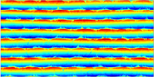
To glean some insight into the basics of wave/staircase interaction, we first examine the DNS of a diffusive $(s ={-} 1)$ system in figures 1–3. This experiment consists of two distinct phases. The first (spin-up) phase (figure 1) was initiated by introducing a set of $n = 8$ horizontal layers at rest with homogeneous total temperature and salinity values $({T_{tot}},{S_{tot}})$ in each layer. Small-amplitude random noise was added to those fields to facilitate the development of active diffusive convection. The computational domain size in this experiment was ${L_x} \times {L_z} = 1600 \times 800$, which corresponds to $16\;\textrm{m} \times 8\;\textrm{m}$ for typical oceanographic conditions, and the numerical mesh contained ${N_x} \times {N_z} = 6144 \times 3072$ grid points. The choice of model parameters represents a compromise between the computational cost and our desire to model an effectively unbounded ocean. In studies of diffusive systems, it is common to characterize the background stratification using the inverse density ratio

(3.1)\begin{equation}R_\rho ^{(inv)} \equiv \frac{1}{{{R_\rho }}} = \frac{{\beta {A_S}}}{{\alpha {A_T}}},\end{equation}

and the simulation in figure 1 was performed with $R_\rho ^{(inv)} = 3$, which is generally representative of Arctic staircases (e.g. Kelley et al. Reference Kelley, Fernando, Gargett, Tanny and Ozsoy2003; Timmermans et al. Reference Timmermans, Toole, Krishfield and Winsor2008). The dimensional buoyancy frequency in this case is

(3.2)\begin{equation}{N^\ast } \equiv \sqrt { - \frac{g}{{\rho _0^\ast }}\frac{{\partial {\rho _{bg}}}}{{\partial {z^\ast }}}} = \sqrt {g(\beta {A_S} - \alpha {A_T})} = \sqrt {g\alpha (R_\rho ^{(inv)} - 1)|{A_T}|} = 4.5 \cdot {10^{ - 3}}\;{\textrm{s}^{ - 1}},\end{equation}

and its non-dimensional counterpart reduces to $N = \sqrt {(R_\rho ^{(inv)} - 1)Pr} = 4.5$.

Figure 1.

The spin-up phase of the diffusive DNS. The instantaneous temperature anomaly fields are shown at various times in (a–c). The experimental parameters are: $h = 100$, $R_\rho ^{(inv)} = 3$, $\tau = 0.01$, $Pr = 10,\;{L_x} = 1600,\;{L_z} = 800,\;{N_x} = 6144$ and ${N_z} = 3072$.

Shortly after initiation (figure 1a), the system starts its transition to fully developed diffusive convection, which is manifested first by the formation of diffusive plumes emanating from the interfaces between homogeneous layers (figure 1b). The growth and vertical spreading of diffusive plumes is followed by the establishment of a quasi-steady circulation pattern, characterized by active convective overturns in layers (figure 1c). To ensure that the system reaches statistical equilibrium by the end of the spin-up phase, each simulation of this nature was extended for at least 200 units of time, which is dimensionally equivalent to approximately 60 hours.

To explore the interaction of fully developed staircases with internal waves, the second stage of the experiment was initiated by introducing into the system a large-scale wave

(3.3)\begin{equation}\left. {\begin{array}{@{}c@{}} {{T_w} = {{\hat{T}}_w}\cos (kx + mz),}\\ {{S_w} = {{\hat{S}}_w}\cos (kx + mz),\quad {{\hat{S}}_w} = R_\rho^{(inv)}{{\hat{T}}_w},}\\ {{\psi_w} = {{\hat{\psi }}_w}\cos (kx + mz),\quad {{\hat{\psi }}_w} ={-} \sqrt {Pr\dfrac{{R_\rho^{(inv)} - 1}}{{k{}^2 + {m^2}}}} {{\hat{T}}_w}.} \end{array}} \right\}\end{equation}

The x- and z-wavelengths of this pattern match the size of the computational domain

(3.4a,b)\begin{equation}\frac{{2{\rm \pi} }}{k} = {L_x},\quad \frac{{2{\rm \pi} }}{m} = {L_z},\end{equation}

and therefore (3.3) conforms to the periodic boundary conditions assumed by the model. In the absence of other perturbations and dissipative effects, (3.3) would represent a free ideal wave oscillating at frequency $\omega = k\sqrt {Pr((R_\rho ^{(inv)} - 1)/(k{}^2 + {m^2}))}$.

The wave pattern (3.3) with a relatively low amplitude of ${\hat{T}_w} = 0.01{L_z}$ was instantaneously superimposed on the state in figure 1(c) and the evolution of the resulting system is illustrated in figure 2. Adding the internal wave results in the visible distortion of the staircase (figure 2a), manifested most clearly in the periodic displacement of its interfaces. This large-scale perturbation systematically weakens in time (figure 2b) and largely disappears by $t = 166$ after the initiation of the second stage (figure 2c). To quantify the observed damping, we compute the net perturbation energy contained in the $(k,m)$ harmonic as a function of time. In non-dimensional units, this quantity takes the following form:

(3.5)\begin{equation}{E_{km}} = \frac{1}{4}\left( {Pr\frac{{\hat{\rho }_c^2 + \hat{\rho }_s^2}}{{R_\rho^{(inv)} - 1}} + \hat{u}_c^2 + \hat{u}_s^2 + \hat{w}_c^2 + \hat{w}_s^2} \right),\end{equation}

where ${\hat{u}_{c,s}}$, ${\hat{w}_{c,s}}$ and ${\hat{\rho }_{c,s}}$ represent the amplitudes of the velocity components and density. These amplitudes are evaluated for every output of field variables $(u,w,T,S)$ as follows:

(3.6)\begin{equation}\left. {\begin{array}{@{}c@{}} {{{\hat{u}}_c} = 2{{[u\cos (kx + mz)]}_{xz}},\quad {{\hat{u}}_s} = 2{{[u\sin (kx + mz)]}_{xz}},}\\ {{{\hat{w}}_c} = 2{{[w\cos (kx + mz)]}_{xz}},\quad {{\hat{w}}_s} = 2{{[w\sin (kx + mz)]}_{xz}},}\\ {{{\hat{\rho }}_c} = 2{{[(S - T)\cos (kx + mz)]}_{xz}},\quad {{\hat{\rho }}_s} = 2{{[(S - T)\sin (kx + mz)]}_{xz}},} \end{array}} \right\}\end{equation}

where symbol ${[ \ldots ]_{xz}}$ denotes the spatial averaging. Using (3.5) and (3.6), the energy was evaluated and recorded for the experiment in figure 2 and ${\textstyle{1 \over 2}}\ln ({E_{km}})$ is plotted as a function of time in figure 3. This plot reveals that, after the initial adjustment period, the internal wave energy starts to decay in an approximately exponential manner. The decay rate $({\lambda _d})$ was computed from the best linear fit to the time record of ${\textstyle{1 \over 2}}\ln ({E_{km}})$, which yielded

(3.7)\begin{equation}{\lambda _d} = 4.35 \cdot {10^{ - 3}},\end{equation}

with the 95 % confidence interval of $\mathrm{\Delta }{\lambda _{ci}} = 1.91 \cdot {10^{ - 4}}$. The corresponding e-folding decay time scale $(\lambda _d^{ - 1})$ is equivalent to 73 wave periods $(2{\rm \pi} /\omega )$, which indicates that the wave interaction with the staircase is relatively weak. This property is exploited in the following asymptotic model (§ 4), which analyses the staircase-induced modification of the ideal wave solution. For representative oceanic parameters (2.6), the dimensional e-folding decay time scale amounts to approximately two days. To confirm that the wave attenuation is caused by its interaction with the staircase, the experiment in figure 2 was reproduced using (3.3) as the initial condition with no staircase present. This simulation, which is also shown in figure 3, resulted in the decay rate of

(3.8)\begin{equation}{\lambda _d} = 3.66852 \cdot {10^{ - 4}},\end{equation}

with the 95 % confidence interval of $\Delta {\lambda _{ci}} = 1.75 \cdot {10^{ - 7}}$. Thus, the wave decay rate in a uniform stratification is an order of magnitude less than in the staircase. In figure 3, we also present the corresponding energy record for the reflected mode with wavenumbers $(k, - m)$. These diagnostics are inspired by a recent model of internal waves incident upon a staircase from remote sources (Sutherland Reference Sutherland2016). Sutherland's theory attributes the adverse action of the staircase to the reflection of waves from high-gradient interfaces, prompting the question of whether the analogous dynamics is realized in the present system. The results in figure 3 indicate that wave reflection does not play a significant role in our simulations. In the course of the experiment in figure 3, the net energy loss by the primary mode $(k,m)$ exceeds the energy gain by the reflected wave $(k, - m)$ by a factor of 430. This finding motivates the search for alternative mechanisms of suppression, which will be identified using the multiscale model in §§ 4 and 5.

Figure 2.

The second phase of the diffusive DNS. The internal wave (3.3) with the amplitude of ${\hat{T}_w} = 0.01{L_z}$ is superimposed on the fully developed state in figure 1(c). The instantaneous temperature anomaly fields are shown at various times in (a–c).

Figure 3.

The solid curve represents the temporal record of ${\textstyle{1 \over 2}}\ln ({E_{km}})$ for the simulation in figure 2, where ${E_{km}}$ is the perturbation energy contained in the mode $(k,m)$. The best linear fit for this record is indicated by the dashed line. The dotted line represents the corresponding pattern for the experiment without the staircase, in which the wave decay is less rapid. Also shown (the dash-dot grey curve) is the corresponding time series for the reflected wave $(k, - m)$.

Figures 4–6 present the corresponding calculation performed in the fingering regime $(s = 1)$. This configuration presents a major computational challenge even in two dimensions since structurally stable fingering staircases are only realized for sufficiently large step heights $h\,\gtrsim\,200$ (Radko Reference Radko2014). Fingering simulations are generally more energetic, and therefore the salinity dissipation scale tends to be less than in the corresponding diffusive DNS. Therefore, the fingering experiment in figures 4–6 was performed with the dissipation ratio of $\tau = 0.1$, which is higher than realized in the ocean $(\tau \sim 0.01)$ but still small. Fortunately, the actual value of the diffusivity ratio has a limited influence on fingering dynamics and intensity as long as it is significantly less than unity (e.g. Stern et al. Reference Stern, Radko and Simeonov2001; Radko Reference Radko2008). The step height in the following simulation is $h = 200$, the computational domain size is ${L_x} \times {L_z} = 2400 \times 1200$, the number of layers is $n = 6$ and the mesh contains ${N_x} \times {N_z} = 6144 \times 3072$ grid points.

Figure 4.

The spin-up phase of the fingering DNS. The instantaneous temperature anomaly fields are shown at various times in (a–c). The experimental parameters are: $h = 200$, ${R_\rho } = 1.5$, $\tau = 0.1$, $Pr = 10$, $Pr = 10,\;{L_x} = 2400,\;{L_z} = 1200,\;{N_x} = 6144$ and ${N_z} = 3072$.

The spin-up phase (figure 4) was effectively completed by $t = 200$, resulting in a quasi-equilibrium state (figure 4c). Note that the interfaces realized in the fingering simulation are not as sharp as their diffusive counterparts (cf. figure 1c) but the layered pattern of the staircase is still well defined. Figure 5 illustrates the decay of the wave with the amplitude of ${\hat{T}_w} = 0.01{L_z}$ that was added to the state in figure 4(c). The perturbation systematically weakens in time (cf. figure 5a–c). It is barely visible in the temperature field shown in figure 5(c), which was recorded at $t = 309$. Figure 6 presents the temporal record of ${\textstyle{1 \over 2}}\ln ({E_{km}})$ along with its best linear fit, from which the decay rate was determined to be ${\lambda _d} = 1.55 \cdot {10^{ - 3}}$. This rate is comparable but less than the corresponding value for the diffusive case (figure 3). The reflected harmonic $(k, - m)$ in the fingering simulation is more pronounced than in the diffusive case. Still, the net loss of energy by the primary wave in figure 6 substantially (by a factor of 43) exceeds the energy gain by the reflected wave, which argues against the significant contribution of reflection to wave suppression. To fully explain the dynamics of wave–staircase interaction and efficiently explore the parameter space, we now turn to an asymptotic multiscale model.

Figure 5.

The second phase of the diffusive DNS. The internal wave with the amplitude of ${\hat{T}_w} = 0.01{L_z}$ is superimposed on the fully developed state in figure 4(c). The instantaneous temperature anomaly fields are shown at various times in (a–c).

Figure 6.

The solid curve represents the temporal record of ${\textstyle{1 \over 2}}\ln ({E_{km}})$ for the simulation in figure 5, where ${E_{km}}$ is the perturbation energy contained in the mode $(k,m)$. The best linear fit for this pattern is indicated by the dashed line. The dash-dot grey curve represents the corresponding time series for the reflected wave $(k, - m)$.

4. Multiscale theory

4.1. Model development

The evolution of large-scale internal waves in the staircase is described using the new set of variables $(X,Z,{t_2})$ that are related to the original ones through

(4.1a,b)\begin{equation}(X,Z) = \varepsilon (x,z),\quad {t_2} = {\varepsilon ^2}t,\end{equation}

where $\varepsilon \ll 1$ is the scale-separation parameter. Variables $(x,z,t)$ are used to describe the processes that operate on the scale of staircase steps (h), whereas $(X,Z,{t_2})$ represent the dynamics on the scale of internal waves. To be specific, the small parameter is defined as the ratio of step height and the vertical wavelength of the internal wave

(4.2)\begin{equation}\varepsilon = \frac{h}{{{L_z}}}.\end{equation}

The basic state in the following model consists of z-periodic and x-independent temperature and salinity patterns $\bar{T}(z)$ and $\bar{S}(z)$ representing the layered step-like diffusive $(s ={-} 1)$ stratification.

The assumed x-invariance of staircase properties represents a significant idealization, which lacks some attributes of observed structures, such as convective overturns in mixed layers and double-diffusive microstructure within the interfaces. The small-scale x-dependent patterns are clearly visible in DNS, both diffusive (e.g. figures 1 and 2) and fingering (e.g. figures 4 and 5). Nevertheless, we believe that such an approach can offer a deeper insight into the wave–staircase interaction problem. Aside from the obvious advantages of simplicity and dynamical transparency, it also affords an opportunity to compare predictions of the reduced-dynamics model with more general DNS-based calculations. The differences and similarities in the results will inform us about the relative significance of the processes neglected by the idealized model.

Given the x-invariance of the basic patterns and the absence of any small-scale variability in the primary wave, their interaction is expected to generate secondary patters that are also devoid of small-scale variability in x. Hence, it becomes unnecessary to use the small-scale horizontal variable in the following analysis. The spatial and time derivatives in governing equations (2.4) are therefore replaced as follows:

(4.3a–c)\begin{equation}\frac{\partial }{{\partial x}} \to \varepsilon \frac{\partial }{{\partial X}}\textrm{ },\quad \frac{\partial }{{\partial z}} \to \frac{\partial }{{\partial z}} + \varepsilon \frac{\partial }{{\partial Z}},\quad \frac{\partial }{{\partial t}} \to \frac{\partial }{{\partial t}} + {\varepsilon ^2}\frac{\partial }{{\partial {t_2}}},\end{equation}

and both sets of variables are treated as independent variables.

Using (4.3a–c), governing equations (2.5) are expressed in terms of both small-scale and large-scale variables, resulting in

(4.4)\begin{equation}\left. {\begin{array}{@{}c@{}} {\dfrac{{\partial T}}{{\partial t}} + {\varepsilon^2}\dfrac{{\partial T}}{{\partial {t_2}}} + \varepsilon {J_{Xz}}(\psi ,T) + {\varepsilon^2}{J_{XZ}}(\psi ,T) - \varepsilon \dfrac{{\partial \psi }}{{\partial X}} = {\nabla^2}(T - \bar{T})}\\ {\dfrac{{\partial S}}{{\partial t}} + {\varepsilon^2}\dfrac{{\partial S}}{{\partial {t_2}}} + \varepsilon {J_{Xz}}(\psi ,S) + {\varepsilon^2}{J_{XZ}}(\psi ,S) - \varepsilon R_\rho^{(inv)}\dfrac{{\partial \psi }}{{\partial X}} = \tau {\nabla^2}(S - \bar{S})}\\ {\dfrac{{\partial \varsigma }}{{\partial t}} + {\varepsilon^2}\dfrac{{\partial \varsigma }}{{\partial {t_2}}} + \varepsilon {J_{Xz}}(\psi ,\varsigma ) + {\varepsilon^2}{J_{XZ}}(\psi ,\varsigma ) = Pr\left[ {\varepsilon \dfrac{\partial }{{\partial X}}(T - S) + {\nabla^2}\varsigma } \right]}\\ {\varsigma = {\nabla^2}\psi ,\quad {\nabla^2} \equiv {\varepsilon^2}\dfrac{{{\partial^2}}}{{\partial {X^2}}} + \dfrac{{{\partial^2}}}{{\partial {z^2}}} + 2\varepsilon \dfrac{{{\partial^2}}}{{\partial z\,\partial Z}} + {\varepsilon^2}\dfrac{{{\partial^2}}}{{\partial {Z^2}}}} \end{array}} \right\},\end{equation}

where ${J_{XZ}}(a,b) \equiv (\partial a/\partial X)(\partial b/\partial Z) - (\partial a/\partial Z)(\partial b/\partial X)$ and ${J_{Xz}}(a,b) \equiv (\partial a/\partial X)(\partial b/ \partial z) - (\partial a/\partial z)(\partial b/\partial X)$ are the Jacobians in $(X,Z)$ and $(X,z)$ respectively. To ensure that $(\bar{T},\bar{S})$ represent the steady state, the temperature and salinity equations in (4.4) are augmented by introducing forcing terms $( - {\nabla ^2}\bar{T}, - \tau {\nabla ^2}\bar{S})$. These terms prevent diffusive dissipation of the basic state, thereby representing the action of microscale processes maintaining thermohaline staircases in the ocean.

To analyse the interaction between waves and the staircase, we seek the solution of governing equations in terms of power series in $\varepsilon \ll 1$ as follows:

(4.5)\begin{equation}\left. {\begin{array}{@{}c@{}} {T = \bar{T}(z) + \varepsilon {T_1}(X,z,Z,t,{t_2}) + {\varepsilon^2}{T_2}(X,z,Z,t,{t_2}) + \cdots }\\ {S = \bar{S}(z) + \varepsilon {S_1}(X,z,Z,t,{t_2}) + {\varepsilon^2}{S_2}(X,z,Z,t,{t_2}) + \cdots }\\ {\psi = {\psi_w}(X,Z,t,{t_2}) + \varepsilon {\psi_1}(X,z,Z,t,{t_2}) + {\varepsilon^2}{\psi_2}(X,z,Z,t,{t_2}) + \cdots } \end{array}} \right\},\end{equation}

where ${\psi _w}$ is the leading-order streamfunction component of a large-scale internal wave. We assume the harmonic form for ${\psi _w}$

(4.6)\begin{equation}{\psi _w} = {\hat{\psi }_w}\exp \{ \textrm{i}(KX + MZ - {\omega _0}t - {\omega _2}{t_2})\} ,\end{equation}

where $(K,M) = {\varepsilon ^{ - 1}}(k,m)$ are the large-scale wavenumbers. The zero-order frequency is denoted by ${\omega _0}$, and ${\omega _2}$ is the correction associated with the variation on the slow time scale. The imaginary component of the perturbation frequency measures the rate of wave decay

(4.7)\begin{equation}{\lambda _d} ={-} {\rm Im}(\omega ) ={-} {\rm Im}({\omega _0}) - {\varepsilon ^2}{\rm Im}({\omega _2}).\end{equation}

We substitute (4.5) and (4.6) in governing equations (4.4) and sequentially solve the hierarchy of balances realized at each order in $\varepsilon $ until an explicit expression for ${\omega _2}$ is found. At each order, we retain only terms that are linear in the wave amplitude $({\hat{\psi }_w})$. This linearization with respect to ${\hat{\psi }_w}$ makes it possible to unambiguously determine the linear decay rate of the primary wave, which is one of the principal objectives of the following analysis.

The O(1) balances of (4.4) are trivially satisfied by the combination of primary wave and the staircase. The $O(\varepsilon )$ balances of T–S equations require that

(4.8)\begin{equation}\left. {\begin{array}{@{}c@{}} {{T_1} = ({{\hat{T}}_w} + {{\hat{\psi }}_w}{{\tilde{T}}_1}(z))\exp \{ \textrm{i}(KX + MZ - {\omega_0}t - {\omega_2}{t_2})\} }\\ {{S_1} = ({{\hat{S}}_w} + {{\hat{\psi }}_w}{{\tilde{S}}_1}(z))\exp \{ \textrm{i}(KX + MZ - {\omega_0}t - {\omega_2}{t_2})\} } \end{array}} \right\},\end{equation}

where ${\hat{T}_w} ={-} K{\hat{\psi }_w}/{\omega _0}$ and ${\hat{S}_w} ={-} KR_\rho ^{(inv)}{\hat{\psi }_w}/{\omega _0}$. The coefficients $({\hat{T}_w},{\hat{S}_w})$ represent the amplitudes of temperature and salinity fields in the primary large-scale wave. However, the nonlinear interaction of the primary wave with the small-scale staircase – the interaction represented by terms ${J_{Xz}}(\psi ,T)$ and ${J_{Xz}}(\psi ,S)$ in (4.4) – also produces small-scale $O(\varepsilon )$ components of temperature and salinity. This dynamics is accounted for by the inclusion of auxiliary functions $({\tilde{T}_1},{\tilde{S}_1})$ in (4.8), which satisfy ordinary differential equations

(4.9)\begin{equation}\left. {\begin{array}{@{}c@{}} {\textrm{i}K\dfrac{{\textrm{d}\bar{T}}}{{\textrm{d}z}} - \textrm{i}{\omega_0}{{\tilde{T}}_1} - \dfrac{{{\textrm{d}^2}{{\tilde{T}}_1}}}{{\textrm{d}{z^2}}} = 0}\\ {\textrm{i}K\dfrac{{\textrm{d}\bar{S}}}{{\textrm{d}z}} - \textrm{i}{\omega_0}{{\tilde{S}}_1} - \tau \dfrac{{{\textrm{d}^2}{{\tilde{S}}_1}}}{{\textrm{d}{z^2}}} = 0} \end{array}} \right\}.\end{equation}

A unique solution for auxiliary functions arising at each order in the expansion is determined by requiring their mean value in z to be zero. These functions are represented by complex numbers and their arguments measure the phase shifts of the corresponding flow components relative to the primary large-scale wave ${\psi _w}$. Note that, unlike T–S equations, the vorticity equation at $O(\varepsilon )$ does not reflect the interaction between primary wave and the basic staircase pattern, and therefore we set ${\psi _1} = 0$.

The $O({\varepsilon ^2})$ balances are solved using

(4.10)\begin{equation}\left. {\begin{array}{@{}c@{}} {{T_2} = {{\hat{\psi }}_w}{{\tilde{T}}_2}(z)\exp \{ \textrm{i}(KX + MZ - {\omega_0}t - {\omega_2}{t_2})\} }\\ {{S_2} = {{\hat{\psi }}_w}{{\tilde{S}}_2}(z)\exp \{ \textrm{i}(KX + MZ - {\omega_0}t - {\omega_2}{t_2})\} }\\ {{\psi_2} = {{\hat{\psi }}_w}({{{\tilde{\psi }}_{2w}} + {{\tilde{\psi }}_2}(z)} )\exp \{ \textrm{i}(KX + MZ - {\omega_0}t - {\omega_2}{t_2})\} } \end{array}} \right\},\end{equation}

where $({\tilde{T}_2},{\tilde{S}_2},{\tilde{\psi }_2})$ satisfy

(4.11)\begin{equation}\left. {\begin{array}{@{}c@{}} {2\textrm{i}M\dfrac{{\textrm{d}{{\tilde{T}}_1}}}{{\textrm{d}z}} + \textrm{i}{\omega_0}{{\tilde{T}}_2} + \dfrac{{{\textrm{d}^2}{{\tilde{T}}_2}}}{{\textrm{d}{z^2}}} = 0}\\ {2\textrm{i}M\tau \dfrac{{\textrm{d}{{\tilde{S}}_1}}}{{\textrm{d}z}} + \textrm{i}{\omega_0}{{\tilde{S}}_2} + \tau \dfrac{{{\textrm{d}^2}{{\tilde{S}}_2}}}{{\textrm{d}{z^2}}} = 0}\\ { - \textrm{i}Pr\dfrac{{{\textrm{d}^4}{{\tilde{\psi }}_2}}}{{\textrm{d}{z^4}}} + {\omega_0}\dfrac{{{\textrm{d}^2}{{\tilde{\psi }}_2}}}{{\textrm{d}{z^2}}} - K\,Pr({{\tilde{S}}_1} - {{\tilde{T}}_1}) = 0} \end{array}} \right\}.\end{equation}

The solvability condition that arises at this order requires that

(4.12)\begin{equation}\omega _0^2 = \frac{{{K^2}(R_\rho ^{(inv)} - 1)Pr}}{{{K^2} + {M^2}}}.\end{equation}

In (4.12), we readily recognize the dispersion relation of free non-dissipative internal waves in the linear background gradient, written here in the non-dimensional form. This is an expected result since (4.6) represents is an internal wave with dimensions greatly exceeding the staircase step height. Neither molecular dissipation nor the presence of a staircase influences the evolution of this primary wave at the leading order. Equation (4.12) also implies that ${\rm Im}({\omega _0}) = 0$ and the wave decay (4.7) reduces to

(4.13)\begin{equation}{\lambda _d} ={-} {\varepsilon ^2}{\rm Im}({\omega _2}).\end{equation}

The essential dynamics of staircase-induced suppression is revealed by the third-order balances which imply that

(4.14)\begin{equation}\left. {\begin{array}{@{}c@{}} {{T_3} = {{\hat{\psi }}_w}({{\tilde{T}}_{3w}} + {{\tilde{T}}_3}(z))\exp \{ \textrm{i}(KX + MZ - {\omega_0}t - {\omega_2}{t_2})\} }\\ {{S_3} = {{\hat{\psi }}_w}({{\tilde{S}}_{3w}} + {{\tilde{S}}_3}(z))\exp \{ \textrm{i}(KX + MZ - {\omega_0}t - {\omega_2}{t_2})\} }\\ {{\psi_3} = {{\hat{\psi }}_w}{{\tilde{\psi }}_3}(z)\exp \{ \textrm{i}(KX + MZ - {\omega_0}t - {\omega_2}{t_2})\} } \end{array}} \right\},\end{equation}

where

(4.15)\begin{align}\left. {\begin{array}{@{}c@{}} {\textrm{i}{\omega_0}K({{\tilde{\psi }}_{2w}} + {{\tilde{\psi }}_2})\left( {\dfrac{{\textrm{d}\bar{T}}}{{\textrm{d}z}} - 1} \right) - \dfrac{{{\textrm{d}^2}{{\tilde{T}}_3}}}{{\textrm{d}{z^2}}}{\omega_0} - 2\textrm{i}M{\omega_0}\dfrac{{\textrm{d}{{\tilde{T}}_2}}}{{\textrm{d}z}} + ({K^2} + {M^2} - \textrm{i}{\omega_2}){\omega_0}{{\tilde{T}}_1}}\\ { + \textrm{i}K{\omega_2} - \textrm{i}{{\tilde{T}}_3}\omega_0^2 - \textrm{i}{{\tilde{T}}_{w3}}\omega_0^2 - {K^3} - K{M^2} = 0}\\ {\textrm{i}{\omega_0}K({{\tilde{\psi }}_{2w}} + {{\tilde{\psi }}_2})\left( {\dfrac{{\textrm{d}\bar{S}}}{{\textrm{d}z}} - R_\rho^{(inv)}} \right) - \dfrac{{{\textrm{d}^2}{{\tilde{S}}_3}}}{{\textrm{d}{z^2}}}{\omega_0}\tau - 2\textrm{i}M{\omega_0}\dfrac{{\textrm{d}{{\tilde{S}}_2}}}{{\textrm{d}z}}\tau + ({K^2}\tau + {M^2}\tau - \textrm{i}{\omega_2}){\omega_0}{{\tilde{S}}_1}}\\ { + \textrm{i}K{\omega_2}R_\rho^{(inv)} - \textrm{i}{{\tilde{S}}_3}\omega_0^2 - \textrm{i}{{\hat{S}}_{3w}}\omega_0^2 - {K^3}R_\rho^{(inv)}\tau - K{M^2}R_\rho^{(inv)}\tau = 0}\\ {\Pr \dfrac{{{\textrm{d}^4}{{\tilde{\psi }}_3}}}{{\textrm{d}{z^4}}} + 4\textrm{i}M\,Pr\dfrac{{{\textrm{d}^3}{{\tilde{\psi }}_3}}}{{\textrm{d}{z^3}}} + \textrm{i}\dfrac{{{\textrm{d}^2}{{\tilde{\psi }}_3}}}{{\textrm{d}{z^2}}}{\omega_0} - 2M\dfrac{{\textrm{d}{{\tilde{\psi }}_2}}}{{\textrm{d}z}}{\omega_0} - \textrm{i}K\,Pr({{\tilde{S}}_2} - {{\tilde{T}}_2}) = 0} \end{array}} \right\}.\end{align}

The emergence of the secondary large-scale plane-wave harmonic with the amplitude $({\varepsilon ^3}{\tilde{T}_{3w}},{\varepsilon ^3}{\tilde{S}_{3w}},{\varepsilon ^2}{\tilde{\psi }_{2w}}){\hat{\psi }_w}$ is triggered by the nonlinear interaction between the second-order wave-induced perturbation in the streamfunction and the basic staircase pattern. These interactions are reflected by terms $\textrm{i}{\omega _0}K{\tilde{\psi }_2}(\textrm{d}\bar{T}/\textrm{d}z)$ and $\textrm{i}{\omega _0}K{\tilde{\psi }_2}(\textrm{d}\bar{S}/\textrm{d}z)$ in temperature and salinity equations of (4.15). Importantly, no analogous nonlinear terms arise in the vorticity equation at this order. Since ${\tilde{\psi }_2}$ is not necessarily orthogonal to the basic state, their interaction produces patterns varying on large scales $(X,Z)$. This dynamics is brought to the fore by z-averaging the temperature and salinity equations in (4.15) and solving the resulting equations for $({\tilde{T}_{3w}},{\tilde{S}_{3w}})$

(4.16)\begin{equation}\left. {\begin{array}{@{}c@{}} {{{\tilde{T}}_{3w}} = \textrm{i}K\omega_0^{ - 2}(\textrm{i}{{\tilde{\psi }}_{2w}}{\omega_0} - \textrm{i}{N_T}{\omega_0} + {K^2} + {M^2} - \textrm{i}{\omega_2})}\\ {{{\tilde{S}}_{3w}} = \textrm{i}K\omega_0^{ - 2}(\textrm{i}{{\tilde{\psi }}_{2w}}{\omega_0}R_\rho^{(inv)} - \textrm{i}{N_S}{\omega_0} + {K^2}R_\rho^{(inv)} + {M^2}R_\rho^{(inv)} - \textrm{i}{\omega_2}R_\rho^{(inv)})} \end{array}} \right\},\end{equation}

where $({N_T},{N_S})$ are the nonlinear terms

(4.17a,b)\begin{equation}{N_T} = {\left[ {{{\tilde{\psi }}_2}\frac{{\textrm{d}\bar{T}}}{{\textrm{d}z}}} \right]_z},\quad {N_S} = {\left[ {{{\tilde{\psi }}_2}\frac{{\textrm{d}\bar{S}}}{{\textrm{d}z}}} \right]_z}.\end{equation}

These nonlinear terms, which will be shown to play a critical role in staircase-induced wave suppression, originate from the advective components ${J_{Xz}}(\psi ,T)$ and ${J_{Xz}}(\psi ,S)$ of the T–S equations in (4.4). They are readily interpreted as the result of large-scale vertical divergence of diapycnal eddy fluxes of heat and salt $({F_T},{F_S})$

(4.18)\begin{equation}\left. {\begin{array}{@{}c@{}} {\textrm{i}K{N_T}\exp \{ \textrm{i}(KX + MZ - {\omega_0}t - {\omega_2}{t_2})\} = \dfrac{\partial }{{\partial Z}}{F_T}}\\ {\textrm{i}K{N_S}\exp \{ \textrm{i}(KX + MZ - {\omega_0}t - {\omega_2}{t_2})\} = \dfrac{\partial }{{\partial Z}}{F_S}} \end{array}} \right\},\end{equation}

where

(4.19)\begin{equation}\left. {\begin{array}{@{}c@{}} {{\varepsilon^3}{F_T} = l.o.\{ {{[wT]}_z}\} }\\ {{\varepsilon^3}{F_S} = l.o.\{ {{[wS]}_z}\} } \end{array}} \right\}.\end{equation}

The notation $l.o.\{ \ldots \} $ in (4.19) is used to represent the leading-order component, which in this case is $O({\varepsilon ^3})$. Note that the fluxes in (4.19) are averaged over small scales. This implies that the staircase-induced suppression is ultimately driven by eddy diffusion of temperature and salinity on the scale of staircase steps (h). The analogous effects of eddy viscosity do not appear at this order. The sought after expression for ${\omega _2}$ is obtained as a solvability condition at $O({\varepsilon ^4})$ as follows. The fourth-order balance of the vorticity equation yields

(4.20)\begin{align} & - 4\textrm{i}M\dfrac{{{\partial ^3}{{\tilde{\psi }}_3}}}{{\partial {z^3}}}Pr\omega _0^2 - \omega _0^2(\textrm{i}{\omega _2} + 2{K^2}Pr - 6{M^2}Pr)\dfrac{{{\partial ^2}{{\tilde{\psi }}_2}}}{{\partial {z^2}}} + 2\dfrac{{\partial {{\tilde{\psi }}_3}}}{{\partial z}}M\omega _0^3 \nonumber\\ &\quad - \textrm{i}K{{\tilde{T}}_3}Pr\omega _0^2 + \textrm{i}K{{\tilde{S}}_3}Pr\omega _0^2\nonumber\\ & \quad + \textrm{i}\omega _0^3({K^2} + {M^2}){{\tilde{\psi }}_2} + (\textrm{i}{\omega _2} - {K^2}Pr - {M^2}Pr)({K^2} + {M^2})\omega _0^2\nonumber\\ &\quad - \textrm{i}Pr{K^2}(R_\rho ^{(inv)}{{\tilde{\psi }}_{w2}} - {{\tilde{\psi }}_{w2}} - {N_S} + {N_T}){\omega _0}\nonumber\\ & \quad + \textrm{i}{{\tilde{\psi }}_{w2}}({K^2} + {M^2})\omega _0^3 + Pr{K^2}((1 - R_\rho ^{(inv)}\tau )({K^2} + {M^2}) + \textrm{i}{\omega _2}(R_\rho ^{(inv)} - 1)) = 0. \end{align}

Equation (4.20) is greatly simplified by recognizing that the coefficient of ${\tilde{\psi }_{w2}}$ is exactly zero as long as ${\omega _0}$ satisfies the dispersion relation (4.12). The resulting expression is then averaged in z, taking advantage of the periodicity of ${\tilde{\psi }_2}(z)$ and ${\tilde{\psi }_3}(z)$:

(4.21)\begin{equation}\begin{array}{ccccc} & (\textrm{i}{\omega _2} - {K^2}Pr - {M^2}Pr)({K^2} + {M^2})\omega _0^2 - \textrm{i}Pr{K^2}({N_T} - {N_S}){\omega _0}\\ & \quad + Pr{K^2}((1 - R_\rho ^{(inv)}\tau )({K^2} + {M^2}) + \textrm{i}{\omega _2}(R_\rho ^{(inv)} - 1)) = 0. \end{array}\end{equation}

Finally, (4.21) is solved for ${\omega _2}$ and the result is further simplified using the dispersion relation (4.12)

(4.22)\begin{equation}{\omega _2} = \frac{1}{2}\frac{{({N_T} - {N_S})K\sqrt {Pr} }}{{\sqrt {({K^2} + {M^2})(R_\rho ^{(inv)} - 1)} }} + \frac{\textrm{i}}{2}\frac{{({K^2} + {M^2})(Pr + 1 - (Pr + \tau )R_\rho ^{(inv)})}}{{(R_\rho ^{(inv)} - 1)}}.\end{equation}

At this point, the multiscale analysis is completed, and we revert to the original variables using (4.1a,b). To simplify the transition, we denote $({\tilde{T}_{10}},{\tilde{S}_{10}}) = \varepsilon ({\tilde{T}_1},{\tilde{S}_1})$, ${\tilde{\psi }_{20}} = {\varepsilon ^2}{\tilde{\psi }_2}$, ${N_{T0}} = {[{\tilde{\psi }_{20}}(\textrm{d}\bar{T}/\textrm{d}z)]_z}$, and ${N_{S0}} = {[{\tilde{\psi }_{20}}(\textrm{d}\bar{S}/\textrm{d}z)]_z}$. As a result, the first-order balance (4.9) takes the form

(4.23)\begin{equation}\left. {\begin{array}{@{}c@{}} {\textrm{i}k\dfrac{{\textrm{d}\bar{T}}}{{\textrm{d}z}} - \textrm{i}{\omega_0}{{\tilde{T}}_{10}} - \dfrac{{{\textrm{d}^2}{{\tilde{T}}_{10}}}}{{\textrm{d}{z^2}}} = 0}\\ {\textrm{i}k\dfrac{{\textrm{d}\bar{S}}}{{\textrm{d}z}} - \textrm{i}{\omega_0}{{\tilde{S}}_{10}} - \tau \dfrac{{{\textrm{d}^2}{{\tilde{S}}_{10}}}}{{\textrm{d}{z^2}}} = 0} \end{array}} \right\},\end{equation}

and the second-order vorticity equation in (4.11) reduces to

(4.24)\begin{equation}- \textrm{i}Pr\frac{{{\textrm{d}^4}{{\tilde{\psi }}_{20}}}}{{\textrm{d}{z^4}}} + {\omega _0}\frac{{{\textrm{d}^2}{{\tilde{\psi }}_{20}}}}{{\textrm{d}{z^2}}} - kPr({\tilde{S}_{10}} - {\tilde{T}_{10}}) = 0.\end{equation}

For any given periodic basic patterns $(\bar{T},\bar{S})$, (4.23) and (4.24) are solved for $({\tilde{T}_{10}},{\tilde{S}_{10}},{\tilde{\psi }_{20}})$ using the Fourier transform in z. The decay rate can now be expressed in terms of the original variables as follows:

(4.25)\begin{equation}\begin{array}{ccccc} {\lambda _d} & ={-} {\varepsilon ^2}{\rm Im}({\omega _2}) = \underbrace{{{\rm Im}\left( {\dfrac{1}{2}\dfrac{{({N_{S0}} - {N_{T0}})k\sqrt {Pr} }}{{\sqrt {({k^2} + {m^2})(R_\rho^{(inv)} - 1)} }}} \right)}}_{A}\\ & \quad + \underbrace{{\dfrac{1}{2}\dfrac{{({k^2} + {m^2})({(Pr + \tau )R_\rho^{(inv)} - Pr - 1} )}}{{(R_\rho ^{(inv)} - 1)}}}}_{B}. \end{array}\end{equation}

Equation (4.25) indicates that the weakening of the large-scale wave is controlled by two effects. Term A represents the wave interaction with the staircase – the dominant damping process and the subject of our study. Term B, on the other hand, represents the damping component that is realized even in the absence of the staircase. It is weak, driven entirely by the direct molecular dissipation of the large-scale wave, and can be neglected for most intents and purposes. The relative intensity of wave suppression in the staircase and the corresponding uniform gradient can be quantified using the diagnostic variable

(4.26)\begin{equation}{r_d} = \frac{A}{B},\end{equation}

which will be referred to as the attenuation ratio. As a consistency check, term B can be readily evaluated for the parameters of the experiment in figure 3, which yields $B = 3.66833 \cdot {10^{ - 4}}$. This value agrees with the DNS-based estimate of the decay rate in linear gradient (3.8) remarkably well, with the relative error of only $5.1 \cdot {10^{ - 5}}$. Theory development for fingering staircases $(s = 1)$ closely mimics the foregoing diffusive model, and the counterpart of (4.25) is

(4.27)\begin{equation}{\lambda _d} = {\rm Im}\left( {\frac{1}{2}\frac{{({N_{S0}} - {N_{T0}})k\sqrt {Pr{R_\rho }} }}{{\sqrt {({k^2} + {m^2})({R_\rho } - 1)} }}} \right) + \frac{1}{2}\frac{{({k^2} + {m^2})((Pr + 1){R_\rho } - Pr - \tau )}}{{({R_\rho } - 1)}}.\end{equation}

In the absence of planetary rotation, the expressions for the decay rate in both diffusive and fingering staircases can be readily obtained in three dimensions by replacing k in (4.25) and (4.27) by the total horizontal wavenumber ${k_h} = \sqrt {{k^2} + {l^2}} $.

4.2. Interpretation

To trace and explain the sequence of processes resulting in the staircase-induced wave suppression, we now assume simple explicit patterns for $(\bar{T},\bar{S})$

(4.28)\begin{equation}\left\{ {\begin{matrix} {\bar{T} = {{\bar{T}}_{tot}} + z,}&{{{\bar{T}}_{tot}} ={-} \dfrac{h}{2}\dfrac{{\tanh (\sin ({\rm \pi} z/h)h_i^{ - 1})}}{{\tanh (h_i^{ - 1})}}}\\ {\bar{S} = {{\bar{S}}_{tot}} + R_\rho^{(inv)}z,}&{{{\bar{S}}_{tot}} ={-} \dfrac{h}{2}R_\rho^{(inv)}\dfrac{{\tanh (\sin ({\rm \pi} z/h)h_i^{ - 1})}}{{\tanh (h_i^{ - 1})}}} \end{matrix}} \right.\quad \textrm{for}\; - \frac{h}{2} \lt z \lt \frac{h}{2}.\end{equation}

Parameter ${h_i}$ in (4.28) measures the thickness of high-gradient interfaces relative to the step height (h), and ${h_i}\sim 0.1$ is representative of oceanic staircases, both fingering and diffusive. The basic patterns (figure 7a,b) reflect the step-like structure of observed staircases (e.g. Kelley et al. Reference Kelley, Fernando, Gargett, Tanny and Ozsoy2003). The specific choice (4.28) was motivated by our desire to construct an infinitely smooth profile that would satisfy periodic boundary conditions at $z = ( - h/2,h/2)$ not only by $(\bar{T},\bar{S})$, but also by all their derivatives. However, additional calculations performed with $\tanh (az)$ and $erf(az)$ profiles indicate that the results obtained for the same interfacial thickness are largely insensitive to the profile choice.

Figure 7.

Multiscale model. The assumed total temperature and salinity fields in the unperturbed staircase are shown in (a). (b) shows the corresponding T–S anomalies. The real and imaginary components of the first-order T–S perturbations are shown in (c) and (d) respectively. The temperature (salinity) patterns are indicated by blue (red) curves. Model parameters match those used for the diffusive DNS in figures 1–3: $R_\rho ^{(inv)} = 3,\;Pr = 10,\;\tau = 0.01,\;h = 100,\;{h_i} = 0.1,\;s ={-} 1$.

The following calculation is performed for the parameters used in the foregoing diffusive DNS (figures 1–3). The immediate consequence of wave/staircase interaction is the tilting of high-gradient interfaces by the primary wave, which generates the first-order perturbation temperature and salinity fields $({\tilde{T}_{10}},{\tilde{S}_{10}})$. These functions, obtained by solving (4.23), are shown in figure 7(c,d). The T–S perturbations are localized in the vicinity of interfaces and their real components substantially exceed the imaginary ones. Neglecting ${\rm Im}({\tilde{T}_{10}})$ and ${\rm Im}({\tilde{S}_{10}})$ has no significant effect on the resulting solutions. This property implies that the first-order small-scale T–S perturbations lag the vertical wave velocity $({w_w})$ by approximately a quarter phase, which is a fully expected kinematic consequence of vertical advection of temperature and salinity across high-gradient interfaces.

The laterally non-uniform distribution of buoyancy associated with the first-order perturbation, in turn, induces the secondary circulation as lighter (denser) fluid at a given z-level tends to rise (sink). This secondary pattern is represented by ${\rm Re}({\tilde{\psi }_{20}})$ component in figure 8(a), which was determined by solving (4.24). On its own, this response can affect the frequency of the primary wave but does not lead to its systematic attenuation since it is in phase with the primary large-scale wave. The secondary circulation pattern, however, is also affected by viscous dissipation, represented by the term $- \textrm{i}Pr({\textrm{d}^4}{\tilde{\psi }_{20}}/\textrm{d}{z^4})$ in the vorticity equation (4.24). Molecular friction generates a small (figure 8b) but dynamically essential correction ${\rm Im}({\tilde{\psi }_{20}})$. This circulation component opposes the flow pattern associated with ${\rm Re}({\tilde{\psi }_{20}})$ and lags it by a quarter of a period. The vertical velocities associated with ${\rm Im}({\tilde{\psi }_{20}})$ induce finite vertical advective fluxes of temperature and salinity $( - \bar{T}k\,{\rm Im}({\tilde{\psi }_{20}}), - \bar{S}k\,{\rm Im}({\tilde{\psi }_{20}}))$. The resulting flux convergence patterns (figure 8d) oppose the T–S tendencies of the primary large-scale wave, causing its gradual dissipation.

Figure 8.

Multiscale model (figure 7). The real and imaginary components of the second-order streamfunction perturbation are shown in (a) and (b) respectively. The real and imaginary components of the nonlinear advective terms ${N_{T0}}$ and ${N_{S0}}$ are shown in (c) and (d) respectively. The temperature (salinity) advection terms ${N_{T0}}({N_{S0}})$ are indicated by blue (red) curves.

The foregoing analysis implies that staircases play a catalytic role in damping large-scale waves. The interaction of the large-scale primary wave with the staircase produces new flow patterns that are localized in the vicinity of high-gradient interfaces. The advective fluxes of temperature and salinity associated with those patterns are more effective in damping the primary wave than molecular dissipation acting directly on the primary large-scale wave. At the same time, our interpretation also underscores the role of molecular friction in controlling the action of eddy fluxes of temperature and salinity. For instance, in the inviscid model $(\nu = 0)$, the eddy fluxes would lack the proper phase alignment with the primary wave required for the staircase-induced suppression.

6. Oceanographic implications

The foregoing analysis indicates that the presence of thermohaline staircases tends to suppress free internal waves, but the magnitude of this effect may be limited. This section attempts to offer a more quantitative assessment of the potential ramifications of staircase-induced suppression. To facilitate the interpretation of our results in terms of relevant oceanographic scales, we cast the following discussion in dimensional units. The conversion between the non-dimensional and dimensional quantities is done using representative parameters (2.6). For vertical wavelengths of ${\sim} {10^3}$, which is equivalent to the dimensional scale of $L_z^\ast{\sim} 10\;\textrm{m}$, both DNS (figure 3) and the multiscale theory (figure 11) predict the decay rate of ${\lambda _d}\sim 4 \cdot {10^{ - 3}}$. This estimate corresponds to the dimensional value of $\lambda _d^\ast{\sim} 4 \cdot {10^{ - 6}}\,{\textrm{s}^{ - 1}}$, representing the e-folding decay periods of 2–3 days. Such intervals are generally less than the time scale of synoptic variability of the atmospheric forcing (2–10 days) and the intrinsic mesoscale variability of the ocean (10–30 days). Thus, it is reasonable to assume that the presence of staircases will adversely affect wave components on vertical scales $L_z^\ast{\sim} 10\;\textrm{m}$. However, the decay rate rapidly (nearly quadratically) decreases with increasing wavelength. Therefore, it seems unlikely that the staircases could have much of an impact on waves with vertical scales exceeding $L_z^\ast \gtrsim 20\;\textrm{m}$. On the other hand, the oceanic wave field is dominated by relatively low-order components, with vertical scales of the order of hundreds of metres, generated by the atmospheric forcing and by the interaction of abyssal flows with bathymetry. Thus, the question arises whether the wave-suppression tendency, dynamically interesting as it may be, can substantially influence the oceanic wave environment. Of particular interest is the impact of the staircase-induced suppression on the intensity of irreversible mixing caused by the internal wave overturns.

To address this concern, we turn to the canonical Garrett & Munk (Reference Garrett and Munk1972) spectrum of internal waves in the ocean, denoted hereafter as GM, which is used to reconstruct the representative time series of vertical shear. Our intent is to determine how the suppression of relatively small-scale waves affects shear and, ultimately, the intensity of small-scale mixing. The implementation is identical to the procedure used by Radko et al. (Reference Radko, Ball, Colosi and Flanagan2015) and Radko (Reference Radko2019a). Therefore, only an abbreviated description is given here. The horizontal velocity field is represented by a superposition of internal waves

(6.1)\begin{align} \left.\begin{aligned} {U^\ast }({z^\ast },{t^\ast }) & = {\rm Re} \left[ {\sum\limits_{j = 1}^J {\iint {{a_u}({k_{GM}},{l_{GM}},j)\cos ({m_{GM}}(\,j)z)} } } \right. \nonumber\\ & \quad \left. \exp(\textrm{i}({\theta_u}({k_{GM}},{l_{GM}},j) - {\sigma_{GM}}t))\,\textrm{d}{k_{GM}}\,\textrm{d}{l_{GM}} \vphantom{\sum\limits_{j = 1}^J}\right]\nonumber\\ {V^\ast }({z^\ast },{t^\ast }) & = {\rm Re} \left[ {\sum\limits_{j = 1}^J {\iint {{a_v}({k_{GM}},{l_{GM}},j)\cos ({m_{GM}}(\,j)z)} } } \right. \\ & \quad \left. \exp(\textrm{i}({\theta_v}({k_{GM}},{l_{GM}},j) - {\sigma_{GM}}t))\,\textrm{d}{k_{GM}}\,\textrm{d}{l_{GM}}\vphantom{\sum\limits_{j = 1}^J}\right] \end{aligned}\right\},\end{align}

where j represents vertical mode numbers and $({k_{GM}},{l_{GM}},{m_{GM}})$ are the wavenumbers. The stochastic wave amplitudes $({a_u},{a_v})$ conform to the GM internal wave spectrum and have random initial phase distribution. We assume uniform background stratification, and $({a_u},{a_v})$ are set to zero for frequencies above the buoyancy frequency ${N^\ast }$ and below the Coriolis parameter ${f^\ast }$. The strength of shear is controlled by the maximal vertical mode number J, which is computed by requiring the mean Richardson number

(6.2)\begin{equation}R{i_{mean}} = \frac{{{N^{{\ast} 2}}}}{{{{[U_z^{{\ast} 2} + V_z^{{\ast} 2}]}_t}}},\end{equation}

to match the chosen target value; $R{i_{mean}} = 1$ is used in the following example. It should be mentioned that wave spectra measured in the upper Arctic Ocean (Levine, Paulson & Morison Reference Levine, Paulson and Morison1987) are often characterized by a less rapid decrease of spectral energy with frequency than in the GM model. Nevertheless, we find it instructive to perform our preliminary assessment using the canonical GM spectrum.

Using (6.1), the temporal record of shear was reconstructed at the mid-level $({z^\ast } ={-} 500\;\textrm{m})$ in the ocean of depth $D = 1000\;\textrm{m}$. The calculation was extended in time for ten inertial periods $(2{\rm \pi} /{f^\ast })$ and the results are expressed (figure 16a) in terms of the instantaneous Richardson number $Ri = {N^{{\ast} 2}}/(U_z^{{\ast} 2} + V_z^{{\ast} 2})$. The Richardson number is traditionally used to determine the susceptibility of shear flows to Kelvin–Helmholtz (KH) instability (von Helmholtz Reference von Helmholtz1868; Kelvin Reference Kelvin1871). Non-dissipative flows are KH-unstable if the Richardson number is less than the critical value of $R{i_{cr}} = {\textstyle{1 \over 4}}$ (Richardson Reference Richardson1920; Howard Reference Howard1961; Miles Reference Miles1961). The amplifying perturbations in this regime tend to evolve into fully turbulent billows (e.g. Woods Reference Woods1968; Thorpe Reference Thorpe1971; Smyth, Moum & Caldwell Reference Smyth, Moum and Caldwell2001), which are thought to be one of the principal sources of irreversible diapycnal mixing in the ocean (e.g. Thorpe Reference Thorpe2005).

Figure 16.

Time series of the Richardson number constructed using the GM internal wave spectrum. Time is expressed in terms of inertial periods $2{\rm \pi} /f$. (a) shows the record of Ri for the canonical GM spectrum. The corresponding records for modified spectra, which retain only wave components with vertical wavelengths exceeding 5 m, 10 m, and 20 m, are presented in (b), (c), and (d) respectively.

The time series in figure 16(a) indicate that the flow meets the KH instability conditions very intermittently and infrequently, which is consistent with the statistics of the Richardson number derived from the open ocean measurements (e.g. Monin & Ozmidov Reference Monin and Ozmidov1985; Polzin Reference Polzin1996; Polzin et al. Reference Polzin, Kunze, Toole and Schmitt2003). Overall, the system spends less than 2 % of the time in the unstable regime $(Ri \lt {\textstyle{1 \over 4}})$. Thus, the question arises whether the staircase-induced suppression of relatively small-scale wave components can substantially reduce the likelihood of KH destabilization. To investigate this possibility, the calculation in figure 16(a) was modified by suppressing all spectral components in (6.1) with vertical wavelengths smaller than the chosen length scale $L_{cr}^\ast $. The resulting time series for $L_{cr}^\ast{=} 5\;\textrm{m}$, 10 m and 20 m are shown in figure 16(b–d) respectively.

The calculations in figure 16 point to the potentially critical role that small-scale waves play in generating KH overturns. Even the suppression of harmonics with vertical wavelengths $L_z^\ast \lt 5\;\textrm{m}$ (figure 16b) has a major effect on the statistics of the Richardson number. The mean Richardson number increases from $R{i_{mean}} = 1.0$ in the original GM model to $R{i_{mean}} = 1.91$ and the minimal value increases from $R{i_{min}} = 0.18$ to $R{i_{min}} = 0.27$. The results for $L_{cr}^\ast{=} 10\;\textrm{m}$ in figure 16(c) are even more dramatic: the average and minimal Richardson numbers increase to $R{i_{min}} = 0.49$ and $R{i_{mean}} = 2.63$ respectively. Finally, the suppression of waves with $L_z^\ast \lt 20\;\textrm{m}$ (figure 16d) effectively precludes any possibility of KH destabilization: $R{i_{min}} = 0.88$ and $R{i_{mean}} = 3.90$. These results support our key thesis: the staircase-induced suppression of relatively small-scale waves $(L_z^\ast{\sim} 10\;\textrm{m})$ could substantially impact the ability of internal waves to generate small-scale turbulence and diapycnal mixing in the ocean.