





1 Introduction
Measurement in the social sciences diverges from the straightforward quantification of physical attributes, such as height or weight because the measured traits are latent, existing beyond direct observation. Such measurements consist of a considerable amount of error, which needs to be accounted for, and they often involve multiple raters and/or multi-item instruments. Consequently, a spectrum of statistical and psychometric models and techniques has been developed to analyze measurements in the social sciences (Bartholomew et al., Reference Bartholomew, Steele and Moustaki2008; Martinková & Hladká, Reference Martinková and Hladká2023; Rao & Sinharay, Reference Rao and Sinharay2007). These methodologies include providing proofs of the measurement reliability, and assessing validity by analyzing relationships with criterion variables and by analyzing the internal structure with factor analysis. Given that social science measurement typically entails multiple components such as items (or criteria, raters, occasions, etc.), there is a particular focus on modeling item responses within multi-item measurements and checking the functioning of each individual item.
To make these complex analytical methods more accessible, psychometric researchers often implement newly proposed models and algorithms in freely available programming software such as R, including its widely used packages, such as mirt (Chalmers, Reference Chalmers2012), lavaan (Rosseel, Reference Rosseel2012), or psych (Revelle, Reference Revelle2024). This may, however, still limit the pool of users to those with programming skills.
To further expand the range of the new methods to a broad audience, software tools have been developed that integrate statistical computing with interactive interfaces. One such enabling technology is Shiny, an open-source framework for building web applications in R or Python (Chang et al., Reference Chang, Cheng, Allaire, Sievert, Schloerke, Aden-Buie, Xie, Allen, McPherson, Dipert and Borges2024; Wickham, Reference Wickham2021). It enables users to create dynamic user interfaces (UIs) and responsive visualizations directly from their statistical code, without requiring prior knowledge of web technologies, such as HTML, CSS, or JavaScript. This feature makes Shiny particularly appealing to data analysts and researchers proficient in R, as it lowers the barrier to developing and deploying web-based tools for data exploration and analysis.
Building on this framework and leveraging the shiny package to create interactive web applications directly from R (Chang et al., Reference Chang, Cheng, Allaire, Sievert, Schloerke, Aden-Buie, Xie, Allen, McPherson, Dipert and Borges2024), the ShinyItemAnalysis (SIA) package (Martinková & Drabinová, Reference Martinková and Drabinová2018; Martinková & Hladká, Reference Martinková and Hladká2023) was developed to provide a collection of psychometric tools accessible both through command-line interface (CLI) functions and an interactive application. The interactive SIA application (Figure 1) includes access to various example datasets, supports uploading and analyzing user data, and enables users to download tables and figures. It also offers automated PDF and HTML report generation, facilitating the integration of psychometric analysis into the test development process.
Introduction screen of the interactive SIA application.

Figure 1 Long description
The interface is divided into three main horizontal sections.
1. Header Navigation Bar: A blue bar at the top contains the logo and title ShinyItemAnalysis Test and item analysis. Below this is a secondary navigation row with tabs for Home, Data, Scores, Validity, Reliability, Item analysis, Regression, I R T models, D I F forward slash Fairness, Modules, Reports, a disk icon, and a gear icon. The Modules tab is active, displaying a white dropdown menu with options: About forward slash Module management, and under a Modules sub-heading, EduTest Item Analysis, EduTest Text Analysis, and Computerized Adaptive Tests.
2. Main Content Area: A white central section titled Welcome. It describes ShinyItemAnalysis as an interactive online application for psychometric analysis built on R and shiny. A bulleted list details features including:
• Exploration of total and standard scores in the Summary section
• Analysis of measurement error in the Reliability section
• Correlation structure and criterion validity analysis in the Validity section
• Item and distractor analysis in the Item analysis section
• Item analysis with regression models in the Regression section
• Item analysis by item response theory models in the I R T models section
• Detection of differential item functioning in the D I F forward slash Fairness section
• Additional psychometric methods implemented via add-on modules in the Modules section
3. Footer: A light gray bar at the bottom displays the logo, the text ShinyItemAnalysis Test and item analysis via Shiny | Version 1.5.5, and the copyright 2026 ShinyItemAnalysis. On the right are icons for a globe, GitHub, and C R A N.
SIA’s interactive environment supports both teaching and applied use of psychometric methods, making them more accessible to a broad audience. It includes training sections with automatically graded exercises and serves as an entry point for users new to R. Sample code is provided to bridge the gap between the graphical UI (GUI) and the CLI, demonstrating how to apply SIA functions alongside psychometric packages, such as mirt (Chalmers, Reference Chalmers2012), psych (Revelle, Reference Revelle2024), and difNLR (Hladká & Martinková, Reference Hladká and Martinková2020). Moreover, the interactive SIA application runs as a background job, allowing for using the R console for practicing or modifying selected code at the same time as the application.
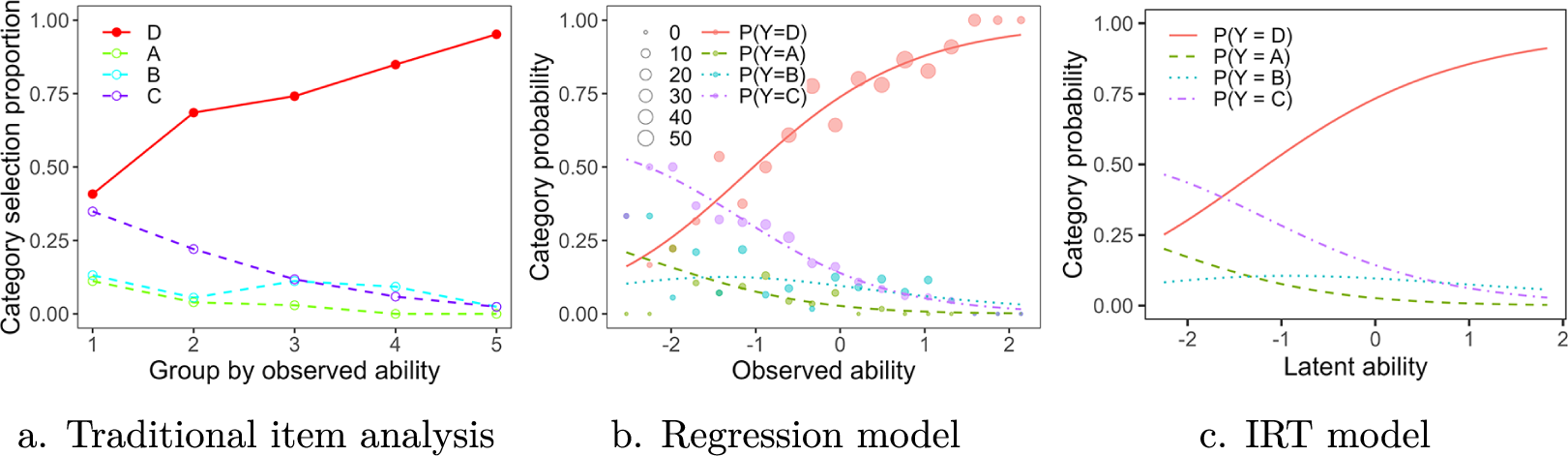
The psychometric analyses within the application are structured in sections, aligning with the workflow outlined in the Standards (AERA, APA, and NCME, 2014) and more closely described by Martinková and Hladká (Reference Martinková and Hladká2023). The main SIA application includes fundamental psychometric models and methods for evaluating multi-item measurement in social sciences, covering evidence of measurement validity, models to assess reliability, and diagnostics for individual item functioning. Further, the application incorporates classical test theory (CTT) and traditional item analysis as foundational methods, and extends these by offering regression models to describe item characteristics and to support the step-by-step development of item response theory (IRT) modeling (Figure 2). Additionally, SIA provides a comprehensive set of tools for differential item functioning (DIF) analysis and also covers other topics, such as computerized adaptive testing (CAT) or text analysis via add-on modules. Together, these features make SIA a powerful platform for complex psychometric analysis.
Different approaches to item analysis on the same item.

Figure 2 Long description
The figure consists of three panels labeled a, b, and c.
Panel a, titled Traditional item analysis, has an x-axis labeled Group by observed ability from 1 to 5 and a y-axis labeled Category selection proportion from 0.00 to 1.00. A solid red line for category D shows a positive linear trend from 0.40 to nearly 1.00. Three dashed lines for categories A, B, and C show downward trends, starting between 0.10 and 0.35 and ending near 0.00.
Panel b, titled Regression model, has an x-axis labeled Observed ability from -2 to 2 and a y-axis labeled Category probability. It features scatter points of varying sizes representing sample sizes from 0 to 50. A solid red line for P(Y equals D) follows a logistic S-curve increasing from 0.20 to 0.95. Dashed lines for P(Y equals A), P(Y equals B), and P(Y equals C) show decreasing probabilities as ability increases.
Panel c, titled I R T model, has an x-axis labeled Latent ability from -2 to 2 and a y-axis labeled Category probability. It shows smooth theoretical curves without data points. The solid red line for P(Y equals D) rises asymptotically toward 1.00. The dashed and dotted lines for categories A, B, and C decrease toward 0.00 as latent ability increases.
Since its release, SIA has seen growing adoption among psychometric researchers, educators, and test developers. Its user-friendly, open-source platform has made it a widely used tool for teaching psychometric concepts and promoting reproducible analyses. While the current user base is concentrated in academia, SIA has also been adopted by test developers, including a national testing agency, to support the development of school admission and leaving exams. The online version of the application has been accessed over 60,000 times from more than 100 countries, and the package has been downloaded more than 120,000 times from RStudio Comprehensive R Archive Network (CRAN) mirror. Thanks to its ongoing development and newly introduced modular design, SIA holds strong potential for broader applications in psychometric consulting or health-care-oriented measurements.
Compared to existing psychometric software, SIA offers a well-integrated and modern interface for both classical and modern test analysis. While some methods, such as structural equation modeling (SEM), are not yet implemented in SIA, the application is distinguished by its open-source nature, active and ongoing development, and high extensibility at the source-code level (see Table 1 for comparison). A central advantage of SIA lies in its flexible extensibility, which allows researchers and methodologists to efficiently incorporate new functionality and tailor the application to evolving analytical needs.
Comparison of interactive psychometric software tools

Table 1 Long description
The table compares ShinyItemAnalysis, jMetrik, WINSTEPS, I R T P R O, Mplus, and flexMIRT.
Columns include:
1. Software name.
2. Open source status.
3. R integration.
4. Extensibility.
5. Implemented methods subdivided into C T T, I R T models, S E M, and D I F.
Key data points:
* ShinyItemAnalysis: Open source Yes; R integration Yes; Extensibility Full code-level; Methods C T T Yes, I R T Dichotomous and polytomous N R M, S E M No, D I F Yes.
* jMetrik: Open source Yes; R integration Yes; Extensibility Minimal; Methods C T T Yes, I R T Dichotomous and polytomous, S E M No, D I F Yes.
* WINSTEPS: Open source No; R integration Partially; Extensibility Limited scripting; Methods C T T Yes, I R T Dichotomous Rasch and polytomous R S M and P C M, S E M No, D I F Yes.
* I R T P R O: Open source No; R integration Partially; Extensibility Basic scripting; Methods C T T No, I R T Dichotomous, polytomous, and multidimensional, S E M No, D I F Yes.
* Mplus: Open source No; R integration Yes; Extensibility Flexible model syntax; Methods C T T No, I R T Dichotomous, polytomous, and multidimensional, S E M Yes, D I F Partial.
* flexMIRT: Open source No; R integration Yes; Extensibility Scripting; Methods C T T No, I R T Dichotomous, polytomous, and multidimensional, S E M No, D I F Yes.
As the field and data complexity undergo a rapid evolution, the ability to adapt and expand analytical tools becomes increasingly important. In response to these demands, we introduce the “SIA modules” framework, a system designed to enable researchers and practitioners to develop add-on SIA modules that seamlessly integrate with and expand upon the capabilities of the main application. In doing so, we take inspiration from jamovi (The jamovi project, 2024), JASP (Love et al., Reference Love, Selker, Marsman, Jamil, Dropmann, Verhagen, Ly, Gronau, Šmíra, Epskamp and Matzke2019), and R packages Rcmdr (Fox, Reference Fox2005), Deducer (Fellows, Reference Fellows2012), and RKWard (Rödiger et al., Reference Rödiger, Friedrichsmeier, Kapat and Michalke2012), all of which offer extension frameworks, thus being similar to our endeavor. Apart from the aforementioned software, both the SIA application and SIA modules are implemented entirely in the R language, keeping it open for the wider R community.
The remainder of this article is structured as follows: Section 2 explains how SIA modules differ from standalone Shiny applications in their structure and connectivity with the main SIA application. It also offers an overview of existing modules housed in the SIAmodules package (Martinková et al., Reference Martinková, Netík and Hladká2026), and examples of modules residing in other packages. Section 3 provides a basic overview of building Shiny applications, together with a demonstration of a standalone Shiny application for CAT simulation. In Section 4, we present a comprehensive guide to SIA module development, including step-by-step instructions. We describe the architecture of SIA modules, how they interact with the core application, what the differences are from the standalone Shiny applications, and we detail the process of developing new modules with the aid of the SIAtools package (Netík & Martinková, Reference Netík and Martinková2026). Finally, Section 5 provides a discussion on the implications of SIA modules and the potential for broader application of the concept across other research areas.
2 SIA modules
While the core SIA application already provides a comprehensive environment for psychometric analyses, its functionality is now being extended through a new modular framework. The recently introduced SIA modules allow researchers and developers to build add-on extensions that integrate directly with the main SIA application. Each module can either introduce new analytical methods or enhance existing ones while fully utilizing the application’s infrastructure for data handling, model estimation, and visualization. This design enables both flexibility and scalability—modules can rely on outputs from the core SIA analyses (e.g., IRT models, factor analysis, or DIF detection), use their own datasets, or even implement computationally intensive procedures based on compiled code. Together, the modular architecture establishes an open, collaborative platform that encourages community contributions and facilitates the dissemination of advanced psychometric tools in an interactive and reproducible form.
2.1 Running SIA with SIA modules
SIA can be run either onlineFootnote 1 or locally within R. To run locally, the SIA package and its dependencies have to be installed in R. The application can then be launched by entering the following single command in the R console:

The function will first check whether all dependencies of the interactive application are satisfied, and offer their installation if not. In this simulated example, the difNLR R package was not installed:

Once all the dependencies are resolved, the run_app() function also checks if there are any SIA modules available on the official SIA repositoryFootnote 2 that are not yet installed and offers to install them. In this case, the function offers a menu of available packages containing SIA modules, among others, the SIAmodules package, which retains a collection of individual modules:

This check is only carried only once per R session and can be disabled completely by setting options(sia.offer_modules = FALSE). Moreover, when run locally, the user may install the modules later on in the GUI as shown in Figure 3. They will become immediately usable without any need to restart the application. If the application runs in the background in a separate R process and a package that contains an SIA module is installed in R library, the user can as well use the “Rediscover modules” button located in the Settings section (under the cogwheel icon in the top right corner) to make the newly installed module available without closing the application.
Installing SIA modules in the interactive application.

2.2 Sample SIA modules
The sample SIA modules presented in this section illustrate the range of possible extensions of the core application. Some operate solely on their own datasets, while others allow interaction with data from the main SIA application or even generate new datasets to be passed back into it.
2.2.1 EduTest Item Analysis: Tailoring data upload, adding data, and model complexity
The EduTest Item Analysis module within the eponymous EduTestItemAnalysis package (Netík & Martinková, Reference Netík and Martinková2024) is specifically tailored to accommodate the format of publicly available Czech Matura Exam data (see the Supplementary Material for sample item data and metadata). It serves as an example of how to create a customized data upload procedure that diverges from the main SIA application. Notably, the EduTest Item Analysis module enables users to upload test metadata specifying the type of each item, i.e., some items may follow the three-parameter logistic IRT model (Birnbaum, Reference Birnbaum, Lord and Novick1968) or its restricted two-parameter logistic (2PL) version, some may be modeled by the generalized partial credit model (Muraki, Reference Muraki1992), and some by the nominal response model (Bock, Reference Bock1972), wherein the correct response must also be specified. This demonstrates the capability to extend the IRT analysis within the SIA application, which currently supports only tests with a single item type. The item-specific IRT modeling is provided in the respective tab of the module, alongside some customized traditional item analyses. Additionally, the module offers the functionality to create binary grouping and/or criterion variables from a factor variable with multiple levels, which can be utilized for DIF detection within the SIA application (Figure 4).
Custom dataset editing in the EduTest Item Analysis module to align with the SIA application format.

Figure 4 Long description
The interface is titled ShinyItemAnalysis Test and item analysis.
At the top, a blue navigation bar contains tabs for Data, Scores, Validity, Reliability, Item analysis, Regression, I R T models, D I F / Fairness, Modules, and Reports. The Modules tab is currently active.
Below the header, the main workspace is titled EduTest Item Analysis with sub-tabs for Data, C T T, and I R T.
In the Data section:
- Item data and Item metadata fields both show a file named mz_2022_spring_l with a blue button labeled Upload complete.
- Options on the right include a checked box for Include only the cases with termín = řádný, prvomaturant, and zkouška_povinna and an unchecked box for Display preview of the data.
The bottom section is titled Use data in the main app. It includes:
- A Group dropdown menu set to smo16.
- Two selection lists: Focal (1) containing highlighted items G Y 4, G Y 6, and G Y 8, and Reference (0) containing highlighted items S T 1 and S T 2.
- A Criterion dropdown menu set to none.
- A large blue button at the bottom left labeled Pass data to S I A.
A small notification at the bottom right corner states Data successfully passed to S I A!
The EduTest Item Analysis module also serves as a non-trivial case study showcasing the module-to-application communication. Upon uploading a dataset to the module, users can modify it to align with the SIA application and reuse it in other tabs beyond the module’s scope. In order to be able to run all the analyses of the SIA application and its other additional modules, users are offered to pass data uploaded and edited in the EduTest Item Analysis module directly to the main application via the “Pass data to SIA” button (see Figure 4).
2.2.2 CAT module: Utilizing models across the application and its modules
The CAT module (Figure 5) from the SIAmodules package simulates an adaptive test with user-defined settings. To start, it generates item responses based on a specified IRT model (dropdown menu) for a respondent of a specified ability (slider). The generated response pattern is presented.
CAT module using the data uploaded in the EduTest Item Analysis module and utilizing the IRT model fitted by the main SIA application.

Figure 5 Long description
The interface is titled Computerized Adaptive Tests.
1. Top Section: I R T model to use is set to S I A-fitted N R M. A slider for Respondent's true ability theta is set to negative 1.5 on a scale from negative 4 to 4.
2. Generated response pattern: A table displays 24 items labeled I 1 through I 24. Binary and polytomous responses are shown, such as 1 for I 1 and 0 for I 2. The text notes a total score of 10 or 33.33 percent correct.
3. C A T post-hoc simulation: Two sliders control the simulation. C A T step is set to 3 of 5. Min. S E is set to 0.4 on a scale of 0 to 1.5. A checkbox is available to show I I Cs for only administered items.
4. Main Visualization: A large plot with multiple axes.
- The left vertical axis represents Ability from negative 4 to 4.
- The right vertical axis represents Ability estimate from negative 4 to 4.
- The bottom horizontal axis is split. The left side shows Information from 0.0 to 2.0. The right side shows Item numbers 0, 18, 13, 10, 8, and 19.
- On the left, blue curves represent item information functions.
- On the right, a blue line graph with circular markers tracks the ability estimate across items, showing a trend starting near negative 1.5 and fluctuating slightly as more items are added. A gray shaded area represents the confidence interval or standard error around the estimate.
- Text overlay indicates: Current ability est. is negative 1.29, Next item is 8, and Next item response is correct.
In each step of the CAT post-hoc simulation, the item with the highest information (displayed in the left plot) at the current ability estimate (shown in the right plot) is presented. Based on the respondent’s answer (correct/incorrect), the ability estimate is updated, and the process repeats until a stopping criterion, defined by the standard error of the ability estimate (left slider), is met.
The module by default offers a 2PL IRT model with predefined item parameters. Moreover, the module offers the possibility to use an IRT model fitted within the main SIA application.Footnote 3 This functionality enables interactive CAT simulations on user-uploaded data, whether provided through the “Data” tab or via another module, such as EduTest Item Analysis. This CAT module is a fully developed version of the simplified example used for the in-depth demonstrations in Sections 3 and 4.
2.2.3 DIF-C: Extending the DIF analysis to a longitudinal setting
Regression-based methods for DIF detection provide the flexibility to incorporate external matching criteria, such as pre-test scores. Consequently, these models can be used to identify so-called DIF in change (DIF-C; Martinková et al., Reference Martinková, Hladká and Potužníková2020) and to analyze item-level heterogeneous treatment effects (Gilbert, Reference Gilbert2024). For instance, in the study on learning competencies (Martinková et al., Reference Martinková, Hladká and Potužníková2020), no overall differences in total scores were observed between students from basic and academic school tracks in either the 6th grade or the 9th grade. Nevertheless, when prior knowledge (6th-grade learning competency scores) was taken into account, certain items in the 9th grade still exhibited differential functioning between the tracks (Figure 6), as identified using the logistic regression model for DIF detection (Swaminathan & Rogers, Reference Swaminathan and Rogers1990).
DIF-C module from the SIAmodules package.

Figure 6 Long description
The interface is a web application titled ShinyItemAnalysis. At the top, a blue navigation bar includes tabs for Data, Scores, Validity, Reliability, Item analysis, Regression, I R T models, D I F / Fairness, Modules, and Reports.
The central content is a scatter plot with two fitted logistic curves. The y-axis is labeled Probability of correct answer, ranging from 0.00 to 1.00. The x-axis is labeled Standardized total score in Grade 6, ranging from -2 to 4.
Data points are represented by circles of varying sizes, where larger circles indicate a higher number of respondents. Yellow circles and a dashed yellow logistic curve represent one group, while blue circles and a solid blue logistic curve represent another. Both curves show a positive logistic trend, but the yellow dashed line sits consistently higher than the blue solid line across the x-axis, indicating a higher probability of a correct answer for the yellow group at the same standardized score levels. The plot is titled Item 6 E _ 9.
A footer at the bottom identifies the software as ShinyItemAnalysis version 1.5.5 with icons for web, GitHub, and R.
While the DIF-C detection is accessible in the main application using the Learning To Learn 9 toy dataset with the score from the 6th grade as an “Observed score” variable, the DIF-C module from the SIAmodules package opens up the core analysis of the study (Martinková et al., Reference Martinková, Hladká and Potužníková2020) in an extended and directly reproducible way. It provides a step-by-step examination of both scores, a summary of the DIF-C analysis, and plots of item characteristic curves (ICCs) for individual items.
2.2.4 Inter-rater reliability: Analyzing ratings from multiple raters
Another aspect of data complexity not currently addressed in the main SIA application involves ratings from multiple raters. When multiple raters are involved, the assessment of inter-rater reliability (IRR) becomes pertinent, typically analyzed through methods, such as analysis of variance or, more generally, variance component models (Martinková et al., Reference Martinková, Bartoš and Brabec2023).
The IRR module (Figure 7) within the SIAmodules package provides an interactive demonstration of the issues of using IRR in restricted-range samples in the context of grant proposal peer review. The module demonstrates that when subsets of restricted-quality proposals are used, this will likely result in zero estimates of IRR under many scenarios, although the global IRR may be sufficient (Erosheva et al., Reference Erosheva, Martinková and Lee2021).
IRR module from the SIAmodules package.

Figure 7 Long description
The interface is titled Range-restricted Reliability within the Shiny Item Analysis application.
At the top, a navigation bar includes tabs for Data, Scores, Validity, Reliability, Item analysis, Regression, I R T models, D I F / Fairness, Modules, and Reports.
Below the introductory text are two interactive controls. On the left, a Proportion slider is set to 70 percent on a scale from 3 to 100. On the right, a Direction dropdown menu is set to top.
The main content consists of two panels.
Left Panel: A scatter plot titled Overall scientific merit score on the y-axis versus Proposal rank on the x-axis. The y-axis ranges from 1 to 5, and the x-axis ranges from 0 to 60. Data points are represented by open circles. A red line with diamond markers shows a general upward trend, with vertical lines indicating range-restricted segments.
Right Panel: A line graph titled Inter-rater reliability on the y-axis versus Proportion of top proposals on the x-axis. The y-axis ranges from 0.00 to 1.00, and the x-axis ranges from 0 percent to 100 percent. The graph shows high variability and higher reliability values at low proportions, dropping to near zero around 70 percent, and then showing a steady upward trend with error bars as the proportion approaches 100 percent. A single black dot marks the current 70 percent selection on the x-axis.
As another example of a module residing in the “Reliability” tab of the main SIA application, the IRR2FPR module of the IRR2FPR package (Bartoš, Reference Bartoš2024) provides an interactive illustration of the calculation of binary classification metrics from IRR, providing an estimate of the probability of correctly selecting the best applicants (Bartoš & Martinková, Reference Bartoš and Martinková2024).
2.2.5 EduTest text analysis: Employing large models and compiled code
EduTest Text Analysis module from the EduTestTextAnalysis (Figure 8) package (Netík et al., Reference Netík, Dlouhá, Martinková and Štěpánek2024) seeks to provide a tool for item difficulty prediction based solely on the item wording (see Štěpánek et al., Reference Štěpánek, Dlouhá and Martinková2023, for the underlying research). The module does not use any data from the main application, nor does it upload any tabular data. Instead, it uses text input fields and the database of several item examples, demonstrating the versatility of the SIA modules pertaining to the input nature.
EduTest Text Analysis module from the EduTestTextAnalysis package.

Figure 8 Long description
The interface is organized into three main vertical sections.
1. Top Navigation Bar: A blue header labeled ShinyItemAnalysis Test and item analysis. Below this is a secondary menu with tabs for Data, Scores, Validity, Reliability, Item analysis, Regression, I R T models, D I F/Fairness, Modules (currently selected), and Reports.
2. Main Content Area: Titled EduTest Text Analysis.
- Item title: A text box containing Free Bus Rides.
- Sample item: A dropdown menu selected on 25, spring 2017.
- Item passage: A large text area containing a story about a 106-year-old woman from Os, Norway, who received an offer for free bus rides due to a computer error reading her birth year 97 as 1997 instead of 1897. The source is listed as w w w dot broadcaster dot org dot u k, upraveno.
- Question: A text box asking Why was the woman offered free bus rides? She was offered free bus rides.
- Correct option: A text box containing because of a computer mistake.
- Incorrect option 1: because she was the oldest person in the town.
- Incorrect option 2: because she wanted to start school.
- Incorrect option 3: because of her hour-long walk to school every morning.
- Action Button: A blue Analyze button is located at the bottom right of this section.
3. Footer: A light gray bar at the bottom containing the ShinyItemAnalysis logo, the text Test and item analysis via Shiny | Version 1.5.5, and copyright 2026 ShinyItemAnalysis. Icons for web, GitHub, and C R A N are on the far right.
Another important feature that this module illustrates is the usage of complex and large models spanning gigabytes of binary data. One of the crucial independent variables in the predictive model is the cosine similarity of different item wording parts (Štěpánek et al., Reference Štěpánek, Dlouhá and Martinková2023), calculated employing the word2vec (Wijffels & Watanabe, Reference Wijffels and Watanabe2023) word embeddings model.
In the module, we implemented a mechanism that can download and cache the compressed binary model from the internet on demand and utilize it immediately in the analysis, thus proving that large and complex models are manageable in the proposed modular architecture. The EduTest Text Analysis module also demonstrates the use of compiled C++ libraries that the word2vec package is wrapping.
3 Building a standalone Shiny application
Before describing how SIA modules can be developed and integrated with the main application, we provide a general introduction to building standalone Shiny applications. We illustrate the process using the CAT simulation, a simplified example resembling the structure and some functionalities of the CAT module described in Section 2.2.2.
3.1 Drafting from R code
Before creating an interactive application, it is often useful to first implement and test the intended functionality as static R code. This ensures that the analysis works as expected before adding the complexity of a Shiny interface. To begin the CAT simulation example, we first load all required libraries.

The CAT simulation relies on an IRT model, for which we consider two options. In the first option, a 2PL IRT model is fitted to the example dataset using the mirt() function. Here, we consider the HCI dataset (Martinková et al., Reference Martinková, Drabinová, Liaw, Sanders, McFarland and Price2017; McFarland et al., Reference McFarland, Price, Wenderoth, Martinková, Cliff, Michael, Modell and Wright2017) from the SIA package, which comprises 20 dichotomously scored items from the Homeostasis Concept Inventory, completed by 651 students (405 males and 246 females).

Long description
The image displays a code block in a monospaced font.
At the top, the first line of code is: data_2pl_mod <- mirt(data = H C I[, 1:20], itemtype = "2PL").
Below this is a comment line: # display the model parameters.
The next line of code is: coef(data_2pl_mod, I R Tpars = TRUE, simplify = TRUE).
Following the code is the output section, prefixed with double hashtags. It begins with ## $items.
Below this is a table with four columns labeled a, b, g, and u. The rows are as follows:
* Item 1: a = 0.851, b = -1.146, g = 0, u = 1.
* Item 2: a = 0.717, b = -1.723, g = 0, u = 1.
* Item 3: a = 1.574, b = -1.526, g = 0, u = 1.
* Item 4: a = 0.347, b = 1.153, g = 0, u = 1.
The output ends with an ellipsis indicating more items follow.
As the second option, we also consider the 2PL IRT model, now with simulated item parameters using the generate.mirt_object() function:

Long description
The script begins with a comment to set the seed for reproducibility followed by the command set dot seed (1678934).
Next, a comment indicates the number of generated items is set to 50, with the variable n underscore items assigned the value 50 L.
A third section simulates 2 P L I R T model parameters using a data frame named pars. It defines a 1 as r l norm (n underscore items, .2, .3) and d as r norm (n underscore items, s d = 1.5).
The fourth section generates the 2 P L I R T model, assigning example underscore 2 p l underscore mod to the function generate dot mirt underscore object (pars, itemtype = ‘2 P L’).
The final section displays the model parameters using the command coef (example underscore 2 p l underscore mod, I R T pars = TRUE, simplify = TRUE).
Below the code is the console output showing a table under the header dollar sign items. The table has columns labeled a, b, g, and u.
* Item dot 1: a = 1.500, b = 0.751, g = 0, u = 1.
* Item dot 2: a = 1.345, b = 0.652, g = 0, u = 1.
* Item dot 3: a = 1.258, b = 1.004, g = 0, u = 1.
* Item dot 4: a = 1.829, b = 0.740, g = 0, u = 1.
The output ends with an ellipsis indicating more items follow.
Next, the Shiny inputs are defined, including the underlying IRT model (here stored in the irt_model object and later to be selectable via a dropdown menu in the intended Shiny app; see Figure 11) and the respondent’s ability (stored in the theta object and adjustable via a slider in the future Shiny app; see Figure 11).

Further, the response pattern for a respondent with the selected ability theta is generated based on the underlying IRT model irt_model using the generate_pattern() function from the mirtCAT package.

In this example, the simulated respondent with the ability equal to 1 would answer the first item incorrectly, the next five items correctly, and so on, assuming the items were administered in a linear format.
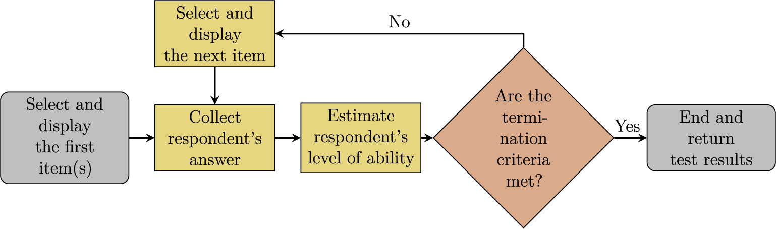
The generated responses are further used in the CAT post-hoc analysis (see Figure 9). In an initial step, before any items are presented to the respondent, their ability is estimated at 0, and the first item is presented to the respondent, choosing the item with the highest information for this ability level. Based on their answer (correct or incorrect, recorded in advance in the generated response pattern), the ability is recalculated from their response and the IRT model. If the standard error of the estimate is above a given threshold (here 0.35), the termination criterion is not yet met, and the cycle repeats. In each subsequent step, the item with the highest information from the remaining pool for the current ability estimate is presented, the ability estimate is updated based on the respondent’s answer, and the termination criterion is checked. This process continues until the termination criterion is met or all items are used, at which point the CAT post-hoc analysis ends.
Flowchart of CAT.

Figure 9 Long description
The process begins on the far left with a grey rectangular box labeled Select and display the first item s. An arrow points right to a yellow box labeled Collect respondent's answer. From here, an arrow points right to another yellow box labeled Estimate respondent's level of ability. This leads to a central brown diamond decision node asking Are the termination criteria met?
Two paths emerge from the diamond. The first path, labeled Yes, points right to a final grey box labeled End and return test results. The second path, labeled No, points upward and then left to a yellow box at the top labeled Select and display the next item. An arrow from this top box points down back into the Collect respondent's answer box, creating a continuous loop until the termination criteria are satisfied.
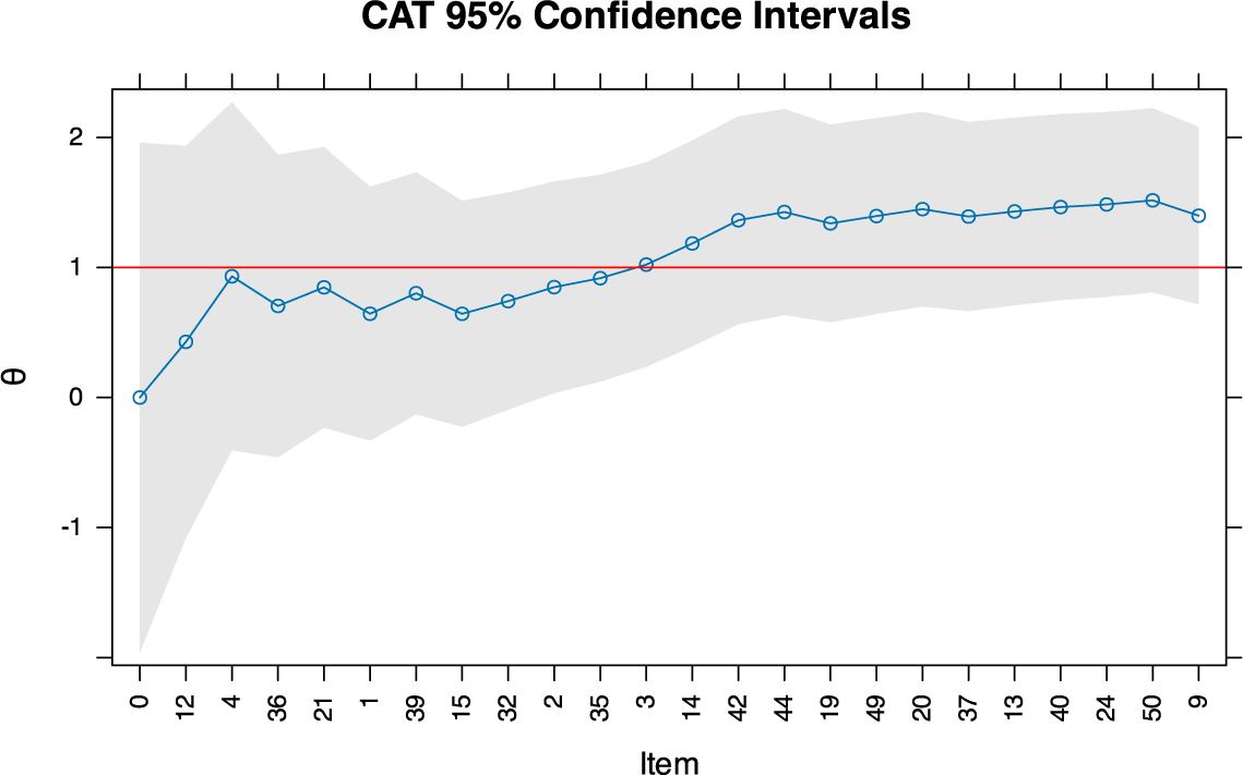
The mirtCAT() function is used to perform this CAT post-hoc analysis, with the underlying IRT model provided via the mo argument, the respondent’s response pattern specified in local_pattern, the first item selection in start_item, subsequent item selection rules set in criteria, and additional parameters such as the termination criterion configuration in design. Once the post-hoc analysis is completed, the basic results are here printed while the adaptive test trajectory can be visualized using the plot() method (see Figure 10).
Trajectory of ability estimates with the 95% confidence intervals for a simulated respondent. The red line corresponds to the ability level used to generate the response pattern in the linear setting, which is subsequently used to simulate the test trajectory in an adaptive setting.

Figure 10 Long description
The line graph is titled C A T 95 percent Confidence Intervals. The horizontal X-axis is labeled Item and contains 25 discrete, non-sequential numeric labels starting from 0 and ending at 9. The vertical Y-axis is labeled with the Greek letter theta and ranges from negative 1 to 2.
* A horizontal red line represents the true ability level, fixed at theta equals 1.
* A light gray shaded area represents the 95 percent confidence interval. This band is very wide at the start (Item 0) and gradually narrows as more items are completed, though it remains wider than the fluctuations of the estimate.
* A blue line with open circular markers tracks the ability estimate. It begins at theta equals 0 for Item 0, shows an initial sharp increase toward the red line, and then exhibits a fluctuating but generally upward trend.
* By Item 3, the blue line crosses the red line and remains slightly above it for the remainder of the test, eventually stabilizing between theta equals 1.4 and 1.5.

Long description
The code block is divided into three sections.
1. Function Call:
sim_res <- mirtCAT(
mo = irt_model,
local_pattern = response_pattern,
start_item = "M I", criteria = "M I",
design = list(min_S E M = .35)
)
2. Console Output:
Two lines prefixed with double hashes show a table with four columns:
n.items.answered: 23
Theta_1: 1.398574
S E.Theta_1: 0.3481323
True.Theta_1: 1
3. Plotting Command:
A comment line reads: # plot with 95% C I (see ?mirtCAT::plot.mirtCAT for further settings).
The final line of code is: plot(sim_res, S E = qnorm(.975)).
In this case, the CAT post-hoc analysis administered 23 items before meeting the termination criterion. The first item presented was item 12, answered correctly by the simulated respondent, which increased their ability estimate and led to the selection of item 4, also answered correctly. This iterative process continued until the final ability estimate of 1.40, obtained after incorrectly answering item 9, was accompanied by a standard error of 0.348, which was just below the 0.35 threshold, at which point the test concluded.
We now turn to transforming this CAT simulation into an interactive Shiny application. Before we begin with the UI part, we must first load all necessary R packages that will be used in the application. We will work in the R script called app.R.Footnote 4

3.2 User interface part
The standalone Shiny application consists of two main R objects: the static UI part and the server function, which are connected through the shinyApp() function. The UI represents the frontend—the part of the application visible to the user in their browser—and is created using the fluidPage() layout function, which specifies the overall structure and arrangement of GUI elements.
In our example, the UI begins with a title panel, followed by an introductory paragraph that describes the application’s functionality:

Next, the dropdown menu is defined using the selectInput() function, allowing the user to choose between two 2PL IRT models. By default, the menu is set to the first model with simulated parameters, while the alternative option corresponds to the model estimated from the HCI dataset:

We also include a slider for setting the respondent’s ability, implemented via the sliderInput() function. This slider allows values ranging from –4 to 4 in steps of 0.1, with a default value of 1. Together with the dropdown menu for selecting the IRT model, these inputs enable users to specify the initial settings for the CAT simulation interactively.

Further, the UI part includes a plot output defined using the plotOutput() function, which links the CAT simulation results generated in the server logic to the UI (see Section 3.3), allowing users to visualize the adaptive test trajectories directly in the application:

Finally, a section with references is included at the bottom of the page as an unordered list, and the UI part is closed with a parenthesis:

Long description
The code is structured as follows:
* h3("References"),
* tags$ul(
* tags$li(
* "Martinkov\‘a, P., & Hladk\‘a, A. (2023). ",
* em("Computational aspects of psychometric methods: With R."),
* " Chapman and Hall/C R C. ",
* a(
* "https://doi.org/10.1201/9781003054313",
* href = "https://doi.org/10.1201/9781003054313"
* )
* )
* )
* )
In addition to the dropdown menu and slider, a wide variety of interactive widgets, i.e., web elements the user can interact with, can be added into the UI. These include action buttons, checkboxes, radio buttons, numeric inputs, text inputs, and more (Wickham, Reference Wickham2021, Chapter 2). Similarly, beyond the plot output displayed in our example, other reactive outputs, such as text displays or tables, may be included to provide dynamic feedback to users (Wickham, Reference Wickham2021, Chapter 3).Footnote 5
3.3 Server part
The server part is the backend of the interactive application—the code that processes user input, runs computations, and returns outputs to be displayed in the browser. It is defined as a function, typically named server, with two main required arguments: input and output. In simple terms, the input object is a list that contains all values entered or selected by the user through the UI. The output object is a list used to store and return the rendered results, such as plots, tables, or text, back to the UI.
Before we define the server function, we must first create the objects that are not “reactive”—i.e., they do not receive any inputs from the user. In our case, this applies to the IRT models. If we were to define the models within the body of the server function, the code would run unnecessarily every time the application was launched.

Long description
The code consists of four main sections, each preceded by a comment starting with a hash symbol.
1. Seed for reproducibility: set dot seed 1 6 7 8 9 3 4.
2. Number of generated items: n underscore items is assigned the value 5 0 L.
3. Simulate 2 P L I R T model parameters: A data frame named pars is created with two columns. Column a 1 uses r l norm with n underscore items, mean log 0.2, and standard deviation log 0.3. Column d uses r norm with n underscore items and standard deviation 1.5.
4. Generate the 2 P L I R T model: example underscore 2 p l underscore mod is assigned the result of generate dot mirt underscore object using parameters equals pars and itemtype equals 2 P L.
5. Fit the 2 P L model on H C I data: data underscore 2 p l underscore mod is assigned the result of the mirt function, taking data from H C I columns 1 to 20 and itemtype equals 2 P L.
Next, we define the server function. Everything that is “reactive” must be specified there. The content of the function can be divided into so-called reactive expressions, which are—in simple terms—functions that automatically update whenever user inputs or any other reactive expressions they depend on change. For instance, the first reactive expression selected_model() depends on the model chosen in the UI via the corresponding irt_model input. Based on the user’s choice, either the 2PL model with generated item parameters (reactive example_2pl_mod()) or the model fitted to the HCI dataset (reactive hci_2pl_mod()) is retrieved:

Another reactive expression (note that we are still inside the server function body), sim_res(), uses both the selected_model() and the ability level specified as the true_theta input in the UI to generate a response pattern and perform a post-hoc CAT analysis. Finally, the renderPlot() function is called on sim_res() to visualize the adaptive test trajectory, and the server function is then closed.

Long description
The code is divided into two main blocks.
First block: sim_res <- reactive({
# get the selected model
mod <- selected_model()
# obtain the response pattern for the given model and selected theta
response_pattern <- generate_pattern(mod, input$true_theta)
# perform post-hoc C A T analysis using the selected mode
mirtCAT(
mo = mod,
local_pattern = response_pattern,
start_item = "M I",
criteria = "M I",
design = list(min_S E M = .35)
)
})
Second block: output$plot <- renderPlot({
plot(sim_res(), S E = qnorm(.975))
})
3.4 Running Shiny application
To create and run the interactive application, the UI and server parts are connected via the shinyApp() function (see Figure 11).

A standalone Shiny application to perform a post-hoc CAT analysis.

Figure 11 Long description
The interface is titled Simulation of Computerized Adaptive Test. Below the title, a text block explains that the module simulates a C A T based on an I R T model.
At the top left, there are two interactive controls. First, a dropdown menu labeled I R T model to use is set to Example 2 P L (simulated). Second, a slider labeled Respondent's true ability is set to a value of 1 on a scale from negative 4 to 4.
The center of the screen features a large line graph titled C A T 95 percent Confidence Intervals. The y-axis is labeled with the Greek letter theta, ranging from negative 1 to 2. The x-axis is labeled Item and lists specific item numbers in the order they were administered: 0, 12, 4, 36, 21, 1, 39, 15, 32, 2, 35, 3, 14, 42, 44, 19, 49, 20, 37, 13, 40, 24, 50, and 6.
A horizontal red line represents the true ability at theta equals 1. A blue line with open circular data points tracks the estimated ability, starting at theta equals 0 for item 0 and gradually converging toward the red line as more items are completed. A light gray shaded area surrounding the blue line represents the 95 percent confidence interval, which is very wide at the start and narrows significantly as the test progresses.
At the bottom, a References section cites Martinková and Hladká (2023) regarding computational aspects of psychometric methods.
4 Extending SIA with add-on modules
4.1 From a standalone shiny application into an SIA module
As outlined above, a standalone shiny application is typically developed using either a single app.R script or separate ui.R and server.R files, which are then deployed to a Shiny server. Alternatively, for a local, server-free setup, the application can be distributed “as-is” within an R package’s inst directory. The latter approach differs substantially from the structure recommended by shiny authors for larger or long-term projects (Wickham, Reference Wickham2021) and from the design adopted by SIA modules and several other packages related to shiny application development, such as golem (Fay et al., Reference Fay, Guyader, Rochette and Girard2023) or rhino (Żyła et al., Reference Żyła, Nowicki, Siemiński, Rogala, Vibal, Makowski and Basa2024).
The main differences from the standalone application approach are as follows: for SIA modules, UI and server parts are both wrapped in dedicated functions that are defined in an R source file inside the R directory of the package. The DESCRIPTION file of a package declares that it contains one or more SIA modules, and finally, a special YAML file stored within the inst directory of the package describes all available SIA modules, including the names of their UI and server functions.
The SIA modules are distributed in ordinary R packages. Developers can create a new package with one or more modules or “append” the modules to their existing packages. Modules available for a package are described in a YAML file, which stores some metadata (title and category) and, crucially, provides bindings to the aforementioned module’s functions.
4.2 Module discovery and usage
Upon launching the application, a mechanism is dispatched to locate SIA modules within R packages installed in the user’s library. Initially, the SIA application collects a list of packages claiming they contain SIA modules. This is declared in the DESCRIPTION file of each module package with

The following code is used in the inst/Modules.R file of the SIA package to collect the names of available packages containing SIA modules:

All such “SIA module” packages are loaded and attached using the standard library() call to ensure that any nontrivial features, such as compiled code or S3/S4 methods, work as usual. A reference to the namespace environment of the currently loaded module package is kept in the ns object. Subsequently, the YAML file of each module package is searched for the modules’ metadata and function bindings. The server function of each module is then located within the package’s namespace environment and invoked using do.call() with the module’s unique identifier as the first argument and with a list of SIA’s reactive, reactiveVal, and reactiveValues as the second argument. This enables the module to reuse any reactive object present in the parent application (see Section 4.3 for more details):

The UI of the module function is called in a similar fashion, but inside shiny’s appendTab() function that appends a new entry to the correct menu:

In the code snippet above, ns refers to the package’s namespace environment, while mod_desc is a list containing the module’s metadata, and mod_id is the unique module identifier created by concatenating the package’s and the module’s names (to prevent name collisions).
The category specified in mod_desc$category within the module’s metadata is used to place the module tab in the desired menu section of the application. Currently, available categories include “Score,” “Validity,” “Reliability,” “Item analysis,” “Regression,” “IRT models,” and “DIF/Fairness.” Any other value assigned to the category attribute will automatically position the module into the “Modules” section of the application.
4.3 Module development with SIAtools
In order to streamline the development of new SIA modules, we introduce a companion package called SIAtools (Netík & Martinková, Reference Netík and Martinková2026). This package comprises a collection of functions for constructing and managing modules, along with ready-to-use templates, guides, and various tests to ensure a smooth integration of the module into the SIA application. It is important to note that developers still retain the option to create SIA modules from scratch, as outlined in previous sections. However, with the assistance of SIAtools, developers can focus solely on the content of the module itself.
Developers interested in creating an SIA module may find themselves in two distinct situations: (1) they possess an existing R package they wish to extend with one or more SIA modules, or (2) they aim to develop a standalone SIA module. In the latter scenario, the SIAtools package offers the capability to create an R package serving as a “container” for the SIA module. This can be achieved either via the R console or through the GUI wizard provided by RStudio. In both cases, developers can utilize the add_module() function to configure the package to be compatible with the SIA application. This function automatically generates an entry in the YAML file and creates a template tailored for a new SIA module. Subsequently, developers are encouraged to fill the template with their code, preview the work in progress with the preview_module() function, and iterate until satisfied with the outcome.
In the following example, we demonstrate the process of extending the SIA application with the SIA module using the companion SIAtools package. We begin by installing the package from CRAN and then loading it:

To create an SIA module from scratch, one may call create_module_project("new_proj") Footnote 6 (where new_proj represents the name of the new RStudio project that will be created in the current working directory). Another way is to use the RStudio project wizard (File > New project > New Directory > ShinyItemAnalysis Module Project). Upon project creation, a welcome message containing basic instructions will pop up.
For the illustration, we will build a simplified version of the CAT module from the SIAmodules package (the resulting simplified module is depicted in Figure 12; the “reference” module is described and shown in Section 2.2.2). Initially, we call add_module("cat") to create a new module within the project. This opens the YAML file (also called “SIA Modules Manifest” in the SIAtools package), which contains the module specification. Within this file, we modify the title to “CAT Example” and define the module’s category (in this instance, “Modules,” see Section 4.2). Following these adjustments, the YAML file should resemble the following:

A preview of the sample CAT module.

Figure 12 Long description
The interface is titled Computerized Adaptive Tests. At the top, a dropdown menu for I R T model to use is set to Module's example 2 P L. Below this, a slider for Respondent's true ability is set to negative 1.5 on a scale from negative 4 to 4.
The main visualization is a line graph titled C A T 95% Confidence Intervals. The y-axis is labeled with the Greek letter theta, ranging from negative 2 to 1. The x-axis is labeled Item and lists eleven specific item numbers: 0, 12, 18, 5, 10, 45, 34, 31, 16, 26, and 43.
A horizontal red line is fixed at theta equals negative 1.5. A blue line with open circular data points represents the estimated ability. It starts at theta equals 0 for item 0 and trends downward, fluctuating slightly before stabilizing near the red line at approximately negative 1.1 by item 43. A light gray shaded area represents the 95% confidence interval, which is very wide at item 0 and narrows significantly as more items are completed, indicating increased precision.
The automatically generated module ID (sm_cat), located in the first row, serves as the identifier for the module throughout the application. Additionally, the function bindings, which direct SIA to the module’s functions, are pre-filled. These functions are housed in sm_cat.R, which is automatically created and opened for the developer in RStudio alongside the edited YAML file. In the sm_cat.R source file, function skeletons are provided with comments and recommended structure, along with placeholder texts indicating where to insert the code for both the server logic and UI components.
Developers can furnish user-facing documentation at the beginning of the sm_cat.R source file. This documentation will be listed along with other functions exported by the package (see ?SIAmodules::sm_cat for an example of the documentation for CAT module living in the SIAmodules package). For instance, the documentation for the simplified example is:

Long description
The code block begins with a header comment # Module documentation followed by a dashed line. Below this is a comment stating # This is the user-facing documentation.
The documentation continues with R oxygen style comments starting with hash and single quote.
- CAT Example
- This S I A module demonstrates basic principles of module development on a simplified version of Computerized Adaptive Tests module from ‘S I A modules’ package.
- @author John Doe
- @references Doe, J. (3024). Sample module. *Journal of Sample Modules, 1*(1), 1--10.
- @name sm_cat
- @family S I A modules
The snippet ends with the keyword NULL.
This documentation offers a brief overview of the module’s purpose and functionality, enhancing clarity for users accessing the package.
The second part of the sm_cat.R file is dedicated to defining the UI function, where developers declare all the components and layout using functions provided by the shiny package.

Long description
The code begins with a header comment ## U I part followed by internal documentation using Roxygen2 tags.
Documentation section:
* @param id: character, the I D assigned by ShinyItemAnalysis.
* @param imports: list of reactive objects exported by ShinyItemAnalysis.
* @param ...: additional parameters.
* @keywords internal.
* @rdname sm_cat_internal.
* @import shiny.
Function definition:
sm_cat_ui <- function(id, imports = N U L L, ...) {
ns <- N S(id) # shorthand for N S(id, inputId)
The function contains a tagList with the following components:
1. h3 header: "Computerized Adaptive Tests".
2. selectInput: labeled "I R T model to use" with choices for "Module's example 2 P L" and "S I A-fitted I R T for binary data".
3. sliderInput: labeled "Respondent's true ability" with a value of 1, minimum of -4, maximum of 4, and step of .1.
4. plotOutput: referencing ns("plot").
The code includes comments advising that any inputId and outputId must be wrapped in an ns() call and suggests using S I A tools::lint_ns() to check for omissions.
Similar to the code presented in Section 3.2, in the code snippet provided above, inside the tagList() function, we included a level 3 heading title, an input element used for the selection of an IRT model, a slider input for adjusting the true ability of a respondent, and the final line refers to the output of this sample module—a plot.
There are some notable differences from the code of the standalone application provided in Section 3.2. An important detail to notice is the usage of the ns() Footnote 7 function around all shiny input and output IDs within the UI function. This function is defined directly in the sm_cat.R source file and ensures that UI input and output IDs match with those expected by their server logic counterparts. The SIAtools package is shipped with a simple linter compatible with the lintr package (Hester et al., Reference Hester, Angly, Hyde, Chirico, Ren, Rosenstock and Patil2023) that checks for the omission of this “namespacing” practice, which can be challenging to debug (for further details, refer to ?module_namespace:linter).
In the third part of the sm_cat.R file, we define the server logic, which, in our case, is done within the sm_cat_server() function.

Long description
The code is contained within a block titled Server part.
At the top, documentation tags include @rdname sm_underscore_cat_underscore_internal and @importFrom mirtCAT generate_underscore_pattern mirtCAT.
The main function is sm_underscore_cat_underscore_server which takes arguments id and imports. Inside, it calls moduleServer and defines ns as session$ns.
There are three main reactive blocks:
1. mod: A reactive switch that selects between example_underscore_2pl_underscore_mod and imports$I R T_underscore_binary_underscore_model based on input$irt_underscore_model.
2. sim_underscore_res: A reactive block that generates a response pattern using generate_underscore_pattern and then calls mirtCAT with parameters mo equals mod, local_underscore_pattern equals response_underscore_pattern, start_underscore_item equals M I, criteria equals M I, and a design list with min_underscore S E M set to point 4.
3. output$plot: A renderPlot function that calls plot on sim_underscore_res with S E set to qnorm point 975.
Similar to the code presented in Section 3.3, in the server logic code, we create a reactive expression mod() that depends on the model selected in the corresponding input. As was the case in the standalone application presented in Section 3, one of the options is an IRT model example_2pl_mod with simulated parameters. The second, and default option, however, differs. By default, this SIA module retrieves an example IRT model, previously defined and stored as internal data of the package (see the complete code in file data-raw/example_2pl_mod.R in SampleModulePackage.zip in the Supplementary Material). This allows us to reference the model within our package. The second reactive expression is the output from the simulation of CAT administration itself, based on the response pattern generated using the true latent ability selected with the slider and the IRT model in use. In each step of the iterative CAT algorithm (Figure 9), the simulation will “present” the item with maximal information (MI) for a “current” estimate of the latent ability, and the test will stop when a minimal standard error of 0.40 is reached. In the final segment of the provided code snippet, we call the plot() method of the mirtCAT package (Chalmers, Reference Chalmers2016) to generate a plot of the post-hoc simulation. It is worth noting that every function from external packages must be imported using, for instance, the @importFrom tag and declared in the DESCRIPTION file because we are constructing a formal R package (Wickham & Bryan, Reference Wickham and Bryan2023).
To preview work in progress, simply call the preview_module() function. By default, all roxygen2 (Wickham et al., Reference Wickham, Danenberg, Csárdi and Eugster2024) blocksFootnote 8 automatically convert into the corresponding .Rd R manual files and NAMESPACE entries. The entire package is loaded and attached without requiring any installation in order to streamline the development as much as possible. The module’s functions are called within a simple shiny application skeleton (see ?preview_module for more details), and when executed, the application launches (see Figure 12).
The module, by default, utilizes the aforementioned example IRT model (Figure 12). However, it is important to note that an error message would be displayed if we selected another model from the SIA application. This occurs because—referring to the source code of the module’s server logic—the module attempts to utilize the imports$IRT_binary_model() reactive, which does not exist. That is because, in the preview, there is no connection to the SIA application, resulting in the imports argument of the sm_cat_server() function being NULL. Footnote 9
To test the module fully connected to the parent SIA application, we have to build the package from source and install it as any other R package. Then, once we run the application locally with ShinyItemAnalysis::run_app(), our module will appear in the Modules tab (as specified in the YAML file), and we can test it with the IRT model fitted by the SIA application. Now, the module receives the imports list of reactives populated by the running SIA application and is able to utilize an IRT model from the SIA application, as was demonstrated in Section 2.2.2.
4.4 Module distribution
As outlined earlier, SIA modules are distributed within standard R packages (containing one or more modules). The official repository is located at https://shinyitemanalysis.org/repo/. Users can install these packages using the conventional install.packages() function and this URL provided in repos argument. Since the repository hosts only the packages of interest without any external dependencies, users need to provide their usual CRAN mirror to ensure the proper installation of the module packages. For instance, to install the SIA module contained in the EduTestItemAnalysis package, which is not available from CRAN, the following code can be used:

The list of already available module packages with detailed information is available at https://shinyitemanalysis.org/repo/. In the R console, users or developers can obtain the list using the following code:

5 Summary and discussion
In this article, we have outlined the process of developing new add-on modules for the SIA interactive application in R with a focus on extending tools for psychometric analysis, with the help of the SIAtools package. We demonstrated fundamental principles and flexible options within the SIA framework using several modules that are already available and of varying complexity.
Interactive Shiny applications have the potential to expand the user community — particularly applied psychometric researchers and educators— and when R code is provided, these applications lower the barrier to adopting R-based workflows. The modular platform we introduced for add-on packages, utilized in the SIA framework, promotes open collaboration, reproducibility, and customization of shiny-based psychometric tools.
The main benefit of the add-on modules lies in their ability to enhance the extensive capabilities and functionalities of the ShinyItemAnalysis package, namely, with contemporaneous methods and models or didactic showcases. This package offers numerous features, including toy datasets, the option to upload custom datasets, a variety of functions utilized in the interactive application, and the possibility to generate automatic reports, among others. As we have demonstrated with the CAT example module, several modules of the SIAmodules package, and with the EduTest Item Analysis and EduTest Text Analysis modules, SIA add-on modules can leverage datasets provided by the SIA application but also use their own ones, up to large complex models or data processed with efficient C++ libraries. Furthermore, they can extend beyond the data types offered in the main SIA application. These modules can seamlessly integrate with the main application; for instance, as we have demonstrated, one module may pass data to the main application for analysis and subsequently transfer the resulting model to another add-on module for further analysis and interactive presentation of the results (e.g., post-hoc analysis of adaptive test), and it does all of this automatically under the hood thanks to reactivity principles of shiny.
To the best of our knowledge, only jamovi (The jamovi project, 2024) and JASP (Love et al., Reference Love, Selker, Marsman, Jamil, Dropmann, Verhagen, Ly, Gronau, Šmíra, Epskamp and Matzke2019) currently offer the possibility to fully or partially access their analyses programmatically from within the R console. This is enabled by their reliance on underlying R packages (the jmv package (Selker et al., Reference Selker, Love and Dropmann2023) for jamovi, and various packages for JASP). Nevertheless, both platforms are primarily designed to be run as a standalone software with GUI in the first place, with programmatic access being a secondary, albeit valuable, feature.
We offer the SIAtools package as a resource to facilitate SIA module development. A similar toolkit is provided in the jmvtools package (Love, Reference Love2024), which also provides a few templates and crucially uses a proprietary compiler to create a module that can be used in the jamovi software with a GUI. On top of that, jmvtools needs a special JavaScript runtime environment to operate. This is also the case for another similar package called jaspTools (de Jong & van den Bergh, Reference de Jong and van den Bergh2024), which relies on a number of external dependencies as well. In contrast, the SIAtools works solely within the realm of the R language.
One of the key advantages of the SIA framework is its open-source nature, which aligns with the principles of open science and reproducible research. The ShinyItemAnalysis package is licensed under the GNU General Public License version 3 (Free Software Foundation, 2007), a copyleft license that ensures end users’ freedom to use, study, share, and modify the software. Under the terms of this license, modules that are derived from or tightly integrated with SIA, such that they form a combined work, must also be distributed under GPL-3. Contributors are therefore encouraged to consider licensing compatibility when developing new modules, especially if they rely on tight integration with the core SIA application.
There are several aspects worth considering in the development of the SIA ecosystem and in future versions of the ShinyItemAnalysis, SIAtools, and SIAmodules packages. The SIAtools package, as well as the broader ecosystem, workflows, and development support for contributors, could be further refined in terms of module testing, building, and submitting to maintain rigor and quality in future contributions. While some recent modules, such as EduTest Item Analysis, combine multiple topics to support specific workflows, e.g., extensions to data upload, traditional item analysis, and more complex IRT models, future development may benefit from separate modules positioned in their respective sections of SIA. In the future, the automatic generation of PDF and HTML reports may offer an editable version that includes outputs from the modules. Further automation of report generation via a command-line environment could foster automation, reproducibility, and reuse with other packages.
While the planned improvements would further enhance the SIA ecosystem, the current suite of ShinyItemAnalysis, SIAtools, and SIAmodules packages already establishes a robust and openly accessible framework. Its GUI can be especially valuable for applied researchers who may lack experience with R or other statistical programming environments, enabling them to conduct advanced psychometric analyses without steep technical barriers. For methodologists and developers, the framework offers a straightforward path to make their methods available interactively, complementing existing R packages with an accessible front end. By fostering openness, not only to users but also to contributors, SIA has evolved into a collaborative ecosystem that can support innovation, reproducibility, and the broader dissemination of psychometric methods.
Supplementary material
Supplementary material, including the accompanying R scripts, is available at https://osf.io/cnbrh/.
Acknowledgements
The authors thank the editor, associate editor, and three anonymous reviewers for their constructive comments on earlier versions of the manuscript. The authors also acknowledge the (co)authors of SIA modules and participants in the short courses “Development of Interactive Shiny Modules for Psychometric Research Dissemination” at IMPS 2025 and “Building Interactive Shiny Modules for Analysis and Dissemination of Social Science Research” at ICS CAS for their valuable feedback.
During the preparation of this work, the authors used generative AI for English proofreading of parts of the article. The authors reviewed and edited the generated content as needed and take full responsibility for the content of the publication.
Funding statement
The study was funded by the Czech Science Foundation project 25-16951S “Complex analysis of educational measurement data to understand cognitive demands of assessment tasks,” by the project “Research of Excellence on Digital Technologies and Wellbeing CZ.02.01.01/00/22_008/0004583” which is co-financed by the European Union, and by the institutional support RVO 67985807.
Competing interests
The authors declare none.





 Open access

